Approximate Inference with the Variational Hölder Bound

Abstract

We introduce the Variational Hölder (VH) bound as an alternative to Variational Bayes (VB) for approximate Bayesian inference. Unlike VB which typically involves maximization of a non-convex lower bound with respect to the variational parameters, the VH bound involves minimization of a convex upper bound to the intractable integral with respect to the variational parameters. Minimization of the VH bound is a convex optimization problem; hence the VH method can be applied using off-the-shelf convex optimization algorithms and the approximation error of the VH bound can also be analyzed using tools from convex optimization literature. We present experiments on the task of integrating a truncated multivariate Gaussian distribution and compare our method to VB, EP and a state-of-the-art numerical integration method for this problem.

1 Introduction

Many Bayesian machine learning problems involve an intractable sum or integral, for which numerical approximations methods have been derived. Approximate Bayesian inference techniques can be broadly classified into sampling-based (e.g. Markov chain Monte Carlo) and optimization-based (e.g. variational Bayes, expectation propagation) methods. While sampling techniques are widely used to explore the space and compute the statistics of interest for the problem, they are not always satisfying due to their stochastic nature and it is hard to assess convergence.

Many algorithms involve the computation an objective function, such as a loss function, a negative log-likelihood or a energy criterion. However, the objective function itself often includes sums that are slow to compute, requiring the approximation of this sum. This is the case in empirical Bayes method (a.k.a. type-II maximum likelihood), mixture models with a latent state space such as high-order hidden Markov models and restricted Boltzmann machines, or even a simple Maximum Likelihood (ML) with fully observed data: the ML estimator of exponential family models with non-standard feature functions requires the computation of the partition-function, which is intractable as soon as the feature functions or the parameter space do not belong the restricted class of tractable models, including Gaussian distributions and tree-structure graphical models for non-Gaussian distributions. For other models, the partition function needs to be approximated and a full set of approximate inference algorithms have been designed during the last decades in including pseudo-likelihood approaches (Gourieroux et al., 1984), but these approaches do not show good empirical performances and do not really help to predict the likelihood of the observations. For other approximation schemes based on mean field approximations, obtaining algorithms with provable polynomial-time convergence guarantees and other theoretical guarantees is hard in general (Wainwright and Jordan, 2008).

In Bayesian statistics, many deterministic inference approaches have been proposed, the main ones being Variational Bayes (VB) (Williams and Hinton, 1991; Jordan et al., 1999; Attias, 2000), Expectation-Propagation (EP) (Minka, 2005), and Tree-Reweighted sum-product (TRW) (Wainwright et al., 2005). For continuous variables, classical approximate inference schemes are based on EP or the Variational Gaussian (VG) representation, which is basically the information inequality applied to the Gaussian case (Challis and Barber, 2011). However, the VG bound is known to be a crude inequality which tends to under estimate the variance, leading to poor results in situations where variance estimates are crucial, for example in Bayesian experimental design (Seeger and Nickisch, 2011). More interestingly, Liu and Ihler (2011) showed that new inference algorithms can be obtained by minimizing the generalized Hölder’s inequality applied on the partition function of a discrete graphical model. Such algorithms do not suffer from the zero-avoiding behavior of VB and the lack of convergence guarantees of EP, and has strong connections with the TRW convex upper bound to the partition function.

In this work, we introduce the Variational Hölder (VH) inequality, a family of tractable upper bounds to the product of potentials, possibly defined on a continuous space, unlike previous work focusing only on the discrete case. Hence, our bound generalizes earlier work by Liu and Ihler (2011) and is simpler in construction. We show that we can infer continuous latent variables values in a Bayesian inference problem where the unnormalized integral is a product of two potentials corresponding to the prior and likelihood respectively. The optimization with respect to the variational parameters in VH is a convex optimization problem and can be solved using off-the-shelf tools. We compare the performance of our method to VB, EP and a state-of-the-art numerical optimizer on the task of integrating a truncated multivariate Gaussian distribution.

2 Variational Hölder bound

Notations

We define a probabilty space $(\Omega,\mathcal{F},\nu)$ where $\Omega$ is a sample space and $\mathcal{F}$ a sigma-algebra defined on it. Let $Z$ be a $\nu$-distributed random variable taking values in a Hilbert space $\mathcal{Z}$. We make use of $\mathcal{L}_{p}$ norms $\|.\|_{p}$ repeatedly, where $p>1$ and $\|f\|_{p}:=\bigl{(}\int{|f(Z)|^{p}}d\nu(Z)\bigr{)}^{\frac{1}{p}}$ for $p<\infty$ and $\|f\|_{\infty}:=\sup_{z}|f(z)|$. Let:

$$I^{*}:=\int{\gamma_{1}(Z)\gamma_{2}(Z)}d\nu(Z)=\|\gamma_{1}\gamma_{2}\|_{1}$$ (1)

be the integral we want to approximate, also called the partition function of the unnormalized distribution with density $\gamma(Z):=\gamma_{1}(Z)\gamma_{2}(Z)$.

Upper bound to the partition function

We define the following functional:

$$\bar{I}_{\bm{\alpha}}(\Psi) :=\|\gamma_{1}\Psi\|_{\alpha_{1}}\|\gamma_{2}/\Psi\|_{\alpha_{2}}$$ (2)

where the argument of $\bar{I}_{\bm{\alpha}}$ is a positive function $\Psi:\mathcal{Z}\mapsto\mathbb{R}^{+}$ which we refer to as the pivot function and ${\bm{\alpha}}=(\alpha_{1},\alpha_{2})\in\mathbb{R}^{+2}$. The main result of this paper is the study of a new inequality to the log-partition function, that we call Variational Hölder (VH) inequality because it corresponds to a direct application of the well-known Hölder’s inequality:

Theorem 1

Let $\gamma_{1}$ and $\gamma_{2}$ be two positive measures defined on $\mathcal{Z}$. The following inequality:

$$I^{*}\leq\bar{I}_{\bm{\alpha}}(\Psi)\enspace,$$ (3)

holds for any positive scalars $\alpha_{1}$ and $\alpha_{2}$ such that $\frac{1}{\alpha_{1}}+\frac{1}{\alpha_{2}}=1$ and any function $\Psi:\mathcal{Z}\mapsto\mathbb{R}^{+}$. Equality holds if for almost all $z\in\mathcal{Z}$, $\Psi(z)=\gamma_{1}(z)^{-\frac{1}{\alpha_{2}}}\gamma_{2}(z)^{\frac{1}{\alpha_{1}}}$.

proof. The bound (1) is obtained using Hölder’s inequality $\|fg\|_{1}\leq\|f\|_{\alpha_{1}}\|g\|_{\alpha_{2}}$ for $f\leftarrow\gamma_{1}\Psi$ and $g\leftarrow\gamma_{2}/\Psi$. The tightness result is given by a direct calculation: $\bar{I}_{\bm{\alpha}}(\gamma_{1}^{-\frac{1}{\alpha_{2}}}\gamma_{2}^{\frac{1}{\alpha_{1}}})=\|\gamma_{1}^{1-\frac{1}{\alpha_{2}}}\gamma_{2}^{\frac{1}{\alpha_{1}}}\|_{\alpha_{1}}\|\gamma_{1}(z)^{\frac{1}{\alpha_{2}}}\gamma_{2}^{1-\frac{1}{\alpha_{1}}}\|_{\alpha_{2}}=\|(\gamma_{1}\gamma_{2})^{\frac{1}{\alpha_{1}}}\|_{\alpha_{1}}\|(\gamma_{1}\gamma_{2})^{\frac{1}{\alpha_{2}}}\|_{\alpha_{2}}=\|\gamma_{1}\gamma_{2}\|_{1}^{\frac{1}{\alpha_{1}}}\|\gamma_{1}\gamma_{2}\|_{1}^{\frac{1}{\alpha_{2}}}=\|\gamma_{1}\gamma_{2}\|_{1}=I^{*}$. $\Box$

The key insight in the VH bound over the standard Hölder bound is that we will choose the pivot function $\Psi$ so that the bound is as close as possible to the target integral. The upper bound on the right-hand side has several useful properties. The first one is that the upper bound can be tractable even if the original quantity $\|\gamma_{1}\gamma_{2}\|_{1}$ is intractable. The second useful property of the log of the bound is convex in $\log(\Psi)$, which makes it convenient to optimize, and in particular using gradient descent methods that are provably convergent in polynomial time. Finally, this bound has theoretical properties that make it suitable for approximating distributions, as shown in the next section.

3 Theoretical Guarantees

In this section, we show that under mild conditions, the VH bound is good for variational inference; when the upper bound is close to the target partition function, then the resulting approximation is also close to the target distribution $p^{*}:=\frac{\gamma_{1}\gamma_{2}}{I^{*}}$.

Proposition 1

For any $\varepsilon>0$, the inequality $I^{*}>(1-\varepsilon)\bar{I}_{\bm{\alpha}}(\Psi)$ implies that:

$$\left\|\frac{(\gamma_{1}\Psi)^{\alpha_{1}}}{\|\gamma_{1}\Psi\|^{\alpha_{1}}_{\alpha_{1}}}-p^{*}\right\|_{2}<\sqrt{2\varepsilon}+\varepsilon\quad \mathrm{if}\quad\alpha_{1}\leq 2,\mathrm{\ and}$$ (4)

$$\left\|\frac{(\gamma_{2}/\Psi)^{\alpha_{2}}}{\|\gamma_{2}/\Psi\|^{\alpha_{2}}_{\alpha_{2}}}-p^{*}\right\|_{2}<\sqrt{2\varepsilon}+\varepsilon\quad \mathrm{if}\quad\alpha_{1}\geq 2\enspace.$$ (5)

The proof is given in the appendix for clarity, but it is novel and is one of the key contributions of the paper. Proposition 1 shows that the smaller the relative gap of the VH inequality is, the better the functions $(\gamma_{1}\Psi)^{\alpha_{1}}$ or $(\gamma_{2}/\Psi)^{\alpha_{2}}$ can approximate the target distribution $p^{*}$. This approximation is useful when $\gamma_{1}\gamma_{2}$ is hard to integrate, but $(\gamma_{1}\Psi)^{\alpha_{1}}$ and $(\gamma_{2}/\Psi)^{\alpha_{2}}$ are easy to integrate.

Now that the approximation properties of the VH bounds have been highlighted, we describe how to effectively use these results in practice.

4 Hölder Variational Bayes

Based on the previous results, we obtain a variational algorithm to approximate product of factors by tractable factors. To do that, we choose the pivot function $\Psi$ in a properly chosen tractable family $\mathcal{F}=\{\Psi(.;\tau),\tau\in\mathcal{T}\}$ where $\mathcal{T}$ is the set of variational parameters that defines the family. Then, we obtain estimates for $\alpha_{1}$ and $\tau$ by minimizing the VH bound (2) over $\mathcal{F}$:

$$(\hat{\tau},\hat{\alpha}_{1})\in\arg\min_{\mathcal{T}\otimes\mathbb{R}}\bar{I}_{\bm{\alpha}}(\Psi(.,;\tau))$$ (6)

Once the optimized values $(\hat{\tau},\hat{\alpha}_{1})$ have been found, the approximation to the exact intractable distribution $p^{*}$ are given by:

$$\hat{p}_{1}(Z):=\frac{(\gamma_{1}(Z)\Psi(Z;\hat{\bm{\tau}}))^{\alpha_{1}}}{\|\gamma_{1}\Psi(.;\hat{\bm{\tau}})\|^{\alpha_{1}}_{\alpha_{1}}}$$ (7)

and

$$\hat{p}_{2}(Z):=\frac{(\gamma_{2}(Z)/\Psi(Z;\hat{\bm{\tau}}))^{\alpha_{2}}}{\|\gamma_{2}/\Psi(.;\hat{\bm{\tau}})\|^{\alpha_{2}}_{\alpha_{2}}}$$ (8)

Other moments can be computed in a similar fashion. Note that by choosing the proper approximating family $\mathcal{F}$, both distributions are assumed to be tractable, i.e. we can compute their normalization constant efficiently. According to Proposition 1, one should choose $\hat{p}_{1}$ or $\hat{p}_{2}$ depending whether $\hat{\alpha}_{1}$ is smaller or greater than 2, but we also considered a convex combination of these two tractable distributions. This amounts to using the following mixture model:

$$\hat{p}_{12}(Z):=\frac{1}{\alpha_{1}}p_{1}(Z)+\frac{1}{\alpha_{2}}p_{2}(Z)\enspace$$ (9)

as an approximating distribution. In their seminal paper, Liu and Ihler (2011) also minimized the Hölder’s bound with respect to parameters and exponent values, but their approach is restricted to discrete graphical models, and they applied this idea in the framework of the bucket elimination algorithm.

So far, the VH bound is very general. It can be applied on discrete and continuous spaces. The sole assumption we made is that $p^{*}\in\mathcal{L}_{1}$, $\gamma_{1}\Psi(:,\tau)\in\mathcal{L}_{\alpha_{1}}$ and$\gamma_{2}\/\Psi(:,\tau)\in\mathcal{L}_{\alpha_{2}}$ for any $\tau\in\mathcal{T}$ and any $\alpha_{k}$ in the range of Hölder’s exponents that are considered. We now turn on to a specific class of functions to illustrate how the VH bound is used in practice.

5 Application: Gaussian Integration

5.1 Problem Definition

Using the notations of the previous section, we define $\gamma_{1}(t)=\prod_{i=1}^{n}f_{i}(t_{i})$ where each function $f_{i}:\mathbb{R}\mapsto\mathbb{R}$ is univariate. We also define $\gamma_{2}(t)$ with $e^{-\frac{1}{2}t^{T}At+b^{T}t}$, where $A$ is a symmetric $n\times n$ matrix and $\bm{b}\in\mathbb{R}^{n}$. We use the Lebesgue measure for $\nu$. Assume we want to evaluate:

$$I^{*}:=\int_{\mathbb{R}^{n}}\prod_{i=1}^{n}f_{i}(t_{i})e^{-\frac{1}{2}\mathbf{t}^{T}A\mathbf{t}+\bm{b}^{T}\mathbf{t}}d\mathbf{t}\enspace.$$ (10)

This type of integral is common in machine learning (Seeger, 2010). Typically, this corresponds to the marginal data probability — a.k.a. the evidence — of a linear regression model with known variance and sparse priors, $n$ being the number of variables. Up to an affine change of variable to obtain orthogonal univariate factors, this integral corresponds also to the data evidence of in a generalized linear model with Gaussian prior, where $n$ is the number of independent observations. The functions $\gamma_{1}$ and $\gamma_{2}$ alone are easy to integrate. This remain true when they are multiplied by a Gaussian potential with diagonal covariance matrices, so that we can choose the following variational family $\{\Psi(\mathbf{t};{\bm{\tau}}),{\bm{\tau}}\in\mathbb{R}^{2n}\}$:

$$\left\{e^{-\frac{1}{2}\mathbf{t}^{T}\mathop{\textrm{diag}}\left({\bm{\tau}}_{1}\right)\mathbf{t}+{\bm{\tau}}_{2}^{T}\mathbf{t}},\quad{\bm{\tau}}_{1}\in\mathbb{R}^{n},{\bm{\tau}}_{2}\in\mathbb{R}^{n}\right\}.$$ (11)

A approximation to the integral (10) is obtained by minimizing the upper bound $\bar{I}_{\bm{\alpha}}$ given in Equation (2).

5.2 Integration of orthogonal univariate function

The first term in the bound $\|\gamma_{1}\Psi(.,{\bm{\tau}})\|_{\alpha_{1}}$ can be obtained efficiently in terms of univariate integrals:

$$\|\gamma_{1}\Psi(.,{\bm{\tau}})\|_{\alpha_{1}}^{\alpha_{1}} = \prod_{i=1}^{n}\int_{\mathbb{R}}f_{i}^{\alpha_{1}}(t_{i})e^{\alpha_{1}(-\frac{\tau_{1i}t_{i}^{2}}{2}+\tau_{2i}t_{i})}dt_{i}$$ (12)

$$= \prod_{i=1}^{n}{U}_{\left[f_{i}\right]}\left(\tau_{1i},\tau_{2i},\alpha_{1}\right)\enspace,$$

where the univariate integrals ${U}_{\left[h\right]}:\mathbb{R}^{2}\times[0;1]\mapsto\mathbb{R}$ are defined as

$${U}_{\left[h\right]}(a,b,\alpha_{1}):=\int_{\mathbb{R}}\left(h(t)e^{-\frac{1}{2}at^{2}+bt}\right)^{\alpha_{1}}dt_{i}\enspace.$$ (13)

Here, $h$ is an arbitrary univariate function $\mathbb{R}\mapsto\mathbb{R}^{+}$. These integrals can be efficiently computed using quadrature integration (e.g. recursive adaptive Simpson quadrature), but in many practical applications, the same functions $f_{i}$ in Equation (12) are used for many factors. A considerable speedup can be obtained by designing integrals dedicated to some functions (in practice, using pre-computed functions with linear interpolation is 10 to 100 times faster than running a new quadrature every time). One important special is the step function: $f_{i}(x)=\mathbb{I}_{\{x\geq 0\}}$ for all $i\in\{1,\cdots,n\}$. For this function and using Gaussian pivot functions as specified in Equation (11), we obtain a closed form expression in terms of normal CDF function $\Phi$:

$${U}_{\left[\mathbb{I}_{\{\cdot\geq 0\}}\right]}(a,b,\alpha) = \sqrt{\frac{2\pi}{\alpha a}}\Phi\left(b\sqrt{\frac{\alpha}{a}}\right)e^{\frac{\alpha b^{2}}{2a}}\enspace.$$ (14)

If there is no truncation in some dimensions, the constant one function gives: ${U}_{\left[\bm{1}\right]}(a,b,\alpha)=\sqrt{\frac{2\pi}{\alpha a}}e^{\frac{\alpha b^{2}}{2a}}.$

5.3 Gaussian Integration

Concerning the other factor $\|\gamma_{2}/\Psi(.,{\bm{\tau}})\|_{\alpha_{2}}$, its log-quadratic form corresponds to a standard Gaussian integral:

$$\|\gamma_{2}/\Psi(.,{\bm{\tau}})\|_{\alpha_{2}}^{\alpha_{2}}=\int_{\mathbb{R}^{n}}e^{-\frac{\alpha_{2}}{2}\mathbf{t}^{T}(A-\mathop{\textrm{diag}}\left({\bm{\tau}}_{1}\right))\mathbf{t}+{\alpha_{2}}(\bm{b}-{\bm{\tau}}_{2})^{T}\mathbf{t}}d\mathbf{t}={(2\pi)^{\frac{n}{2}}}e^{J\left({\alpha_{2}}(A-\mathop{\textrm{diag}}\left({\bm{\tau}}_{1}\right)),{\alpha_{2}}(\bm{b}-{\bm{\tau}}_{2})\right)},$$

where $J(M,v):=-\frac{1}{2}\log|M|+\frac{1}{2}v^{T}M^{-1}v$.

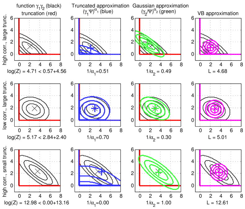
Figure 1: 2D Truncated Gaussian integration. Each row represents a different correlation/truncation setting. From left to right, the columns show 1) the target function $\gamma_{1}\gamma_{2}$, 2) its first tractable approximation $(\gamma_{1}\Psi)^{\alpha_{1}}$ (product of orthogonal univariate function), 3) its second tractable approximation $(\gamma_{2}/\Psi)^{\alpha_{2}}$ (correlated Gaussian distribution) and 4) VB approximation. Symbols ’x’ and ’+’ are the exact and approximate means, respectively.

5.4 Truncated multi-variate Gaussian integration

Most of the truncated multivariate Gaussian integration problems with linear truncations can be put under the canonical form (10) where truncations are orthogonal, i.e. $f_{i}(x)=\mathbb{I}_{\{x\geq 0\}}$ for all $i\in\{1,\cdots,n\}$. Integrating truncated correlated Gaussian is a known open problem for which several approximation techniques have been proposed. In numerical approximation, adaptive quadratures approach have been well investigated (Genz and Bretz, 2009), but are still limited to small dimensions. Approximate inference techniques, such as Expectation-Propagation (EP), have been recently proposed, but the algorithm remains unstable, even after specific improvements to increase the accuracy of the method (Cunningham et al., 2011). One of the reason is the fact that EP does not give any guarantee about the approximation. To be used in a learning framework, upper and lower bounds to the integral (10) are often very useful. We focus here on the upper bound.

Initialization

We need to initialize parameters so that the integral is tractable. This is not always trivial, but in principle, any point in the convex set $\mathcal{T}=\{({\bm{\tau}}_{1}^{T},{\bm{\tau}}_{2}^{T})^{T}\in\mathbb{R}^{2n}|0\prec\mathop{\textrm{diag}}\left({\bm{\tau}}_{1}\right)\prec A\}$ leads to a finite integral. For example, setting $\tau_{1i}$ to half of the minimum Eigen value of $A$ lies within the convex set.

Bound minimization

After simplification, we get the following overall objective for the upper bound of a multivariate truncated Gaussian:

$$\frac{1}{\alpha_{1}}\sum_{i}\log{U}_{\left[f_{i}\right]}(\tau_{1i},\tau_{2i},\alpha_{1})+\frac{1}{\alpha_{2}}J({\alpha_{2}}(A-\mathop{\textrm{diag}}\left({\bm{\tau}}_{1}\right)),{\alpha_{2}}(b-\tau_{2}))-\frac{n}{2}\log(2\pi).$$ (15)

Figure 1 presents results on a two dimensional truncated gaussian integration problem. The optimal value of $\alpha_{1}$ depends on both the level of truncation and the correlation.

6 Comparison with Variational Bayes

6.1 Variational Hölder vs. Variational Bayes

One can compare the VH inequality (3) to the one provided by the Variational Bayes (VB) inequality:

$$\log I^{*}\geq\int\log\gamma_{1}(z)dq(z)+\int\log\gamma_{2}(z)dq(z)+\mathcal{H}(Q)\enspace.$$ (16)

for any distribution $Q$ absolutely continuous with respect to $\nu$, where $\mathcal{H}$ denotes the information entropy and $q=\frac{dQ}{d\nu}$.

VB provides a lower bound to the log-sum-exp function, while the VH provides an upper bound. One disadvantage of the VB bound (16) is that it is not concave in general, leading to objective functions that are difficult to maximize and a bound that does not come with theoretical guarantees. Another disadvantage is that the approximating distribution $Q$ must have a support included in the base distribution $\nu$, which is not always convenient when the target distribution has subspaces with zero probability. This zero-avoiding effect of the VB bound can lead to crude approximations of the original integral (Minka, 2005).

6.2 Variational Bayes for truncated multi-variate Gaussian integration

As a comparison, we consider in this section the VB approach, that gives a lower bound to the likelihood. The key idea to be able to apply VB on this problem is to consider independent truncated Gaussian for the approximation family. We start with (10):

$$\log I^{*}:=\log\int_{\mathbb{R}^{n}}\prod_{i=1}^{n}f_{i}(t_{i})e^{-\frac{1}{2}\mathbf{t}^{T}A\mathbf{t}+\bm{b}^{T}\mathbf{t}}d\mathbf{t}\geq L$$ (17)

where $L$ denotes the negative variational free energy, a.k.a. the variational lower bound, given by

$$L:=\sum_{i=1}^{n}\mathbb{E}_{q}\left[\log f_{i}(t_{i})\right]-\frac{1}{2}\mathop{\textrm{tr}}(A\mathbb{E}_{q}\left[\mathbf{t}\mathbf{t}^{T}\right])+\bm{b}^{T}\mathbb{E}_{q}\left[\mathbf{t}\right]+\mathcal{H}[q]$$ (18)

We choose the variational distribution $q$ to be a product of univariate truncated normal distributions which are truncated at zero. Let $q=\prod_{i}\mathcal{TN}(\mu_{i},\sigma_{i})$. The variational bound is given by

Minimization of the lower bound could be done iteratively by solving one-dimensional truncated Gaussian fits in a round-robin fashion, however, in the experiments below, we computed the gradient of the variational objective and used a gradient descent technique to find the optimal variational parameters.

$\kappa$	$n$	Genz	EP	VB	VH
0.1	5	5.1499	5.1327	2.9489	6.4169
1	5	0.41768	0.41234	0.10715	0.98725
0.1	20	24.7689	24.7702	17.5524	28.2854
1	20	1.9203	1.9196	0.97199	2.8037
0.1	50	66.2055	66.1991	44.3699	68.971
1	50	9.9	9.8999	5.9196	11.2919

$\kappa$	$n$	VB vs EP	VH vs EP	VB vs VH
0.1	5	1.9286	0.35811	1.7518
1	5	0.12856	0.073666	0.19735
0.1	20	3.0963	3.3148	2.9741
1	20	0.19727	0.074579	0.27093
0.1	50	5.5944	0.72705	5.9132
1	50	0.51551	0.076875	0.58154

Table 1: Comparison of log partition function (left) and error in first moment (right)

7 Experiments

To undestand the properties of the VH bound, we compared its properties with existing deterministic integration. integration methods in high dimension. We considered the ground-truth to be the method of Alan Genz (Genz and Bretz, 2009) which is based on a sophisticated technique of pseudo-random number generation. The main interest is that it can give an error estimate of the error, so that we can evaluate precisely the validity of various techniques. We used the matlab code provided by the author. Another efficient technique for integration of truncated Gaussians is based on the use of Expectation-Propagation (EP), as described by Cunningham et al. (2011). In this case as well, a matlab code is provided by the authors. Finally, we used implemented the VB version described above to obtain a lower bound to the true integral. Both VB and VH objectives were minimized using the L-BFGS algorithm provided by matlab fminunc function.

We used multiple correlations settings, where the precision matrix $A$ was obtained using the following rule: $A:=\kappa I+v*v^{T}$, where $v$ is drawn from a $n$-dimensional Gaussian distribution with unit covariance matrix. We varied the correlation by setting $\kappa\in\{0.1,1\}$ and the dimension by varying $n\in\{5,20,50\}$. We also compared the accuracy of the moment computation, since large gap in the bound does not always imply large difference in the results. The method of Genz did not output moments, so we also compared the accuracy of the moment computation by computing the Euclidean norm of the difference between the three methods: EP, VB and VH for the mean of the target distribution.

Table 1 gives the results. The first 4 columns compare the integral values. We can see that VB correctly estimates a lower bound to the true integral, and that VG consistently gives an upper bound. EP seems to be generally very accurate, sometimes over-estimating, sometimes under-estimating the exact integral. An interesting phenomenon is that Holder is more accurate than VB in the high correlation setting ($\kappa=0.1$. This is expected since VB is unable to use correlation due to the fact that the approximating family is composed by independent truncated Gaussian variables.

When comparing the moment computation, we see that Holder can give very accurate results, even if the gap in the bound was large. We also see that the higher the dimension, the better VH becomes with respect to VB. We also notice that the high correlation setting, VH and EP are closer to each other, compared to VB suggesting again, that high correlation are well handled by the VH approximation.

8 Generalization for many factors

Here, we consider the more general case where the integral to compute is the product of $K$ factors, $K>2$: $I^{*}:=\int\prod_{k^{\prime}=1}^{K}f_{k}(z)d\nu(z)$ where $f_{k}$, $k=1,\cdots,K$ are the individual factors. We have the following results:

Theorem 2

The following inequality:

$$I^{*} \leq \prod_{k=1}^{K}\left(\int_{\mathcal{Z}}{\left(\frac{f_{k}(z)}{\Psi_{k}(z)}\right)}^{\alpha_{k}}\prod_{k^{\prime}=1}^{K}\Psi_{k^{\prime}}(z)d\nu(z)\right)^{\frac{1}{\alpha_{k}}}$$ (33)

holds for any ${\bm{\alpha}}=(\alpha_{1},\cdots,\alpha_{K})\in(0,\infty)^{K}$ such that $\sum_{k=1}^{K}\frac{1}{\alpha_{k}}=1$ and any function $\Psi_{k}:\mathcal{Z}\mapsto\mathbb{R}^{+}$ in $\mathcal{L}_{\alpha_{k}}$, $k=1,\cdots,K$.

proof.(sketch) Similarly to the generalization of Hölder’s inequality for a product of functions, we can apply the binary VH bound recursively. $\Box$ One can verify that we recover the results of Section 2 for $K=2$. The VH method can be obtained by parameterizing the pivot functions and minimizing (33) with respect to the pivot functions $\Psi_{k}$ and ${\bm{\alpha}}$. Tightness and approximation properties studied in Section 3 can also be extended to the case of multiple factors.

9 Discussion

We have introduced a new family of variational approximations that are based on the minimization of an upper bound to the log-partition function. We demonstrated that the variational inference problem is convex if the variational function is log-linear, which has great practical and theoretical advantages over mean-field/VB approximations, which is the main approach used today by practitioners. We also provide a novel way to handle Gaussian integration problems. In fact, we could express probit regression as a special case of this problem, and the extension to other distribution is possible in theory. One of the unique feature of this approach is that the approximation maintains the heavy tails, but we still a convex objective. Further experiments will be conducted to evaluate how good this approximation behaves in Bayesian posterior estimation.

The VH framework presented here is very general, and can be applied to many models and optimized using a large variety of algorithms and speedup tricks, similarly to what happened with VB and EP other the last two decades.

We focused mainly on one type of intractable integrals that is common in machine learning problems (GLM or linear models with sparse priors), but the approach is generic and could potentially be applied in many other settings. One of the main area of application is the inference in graphical models with discrete variables, on which the TRW sum-product algorithm has been designed (Wainwright et al., 2005), as well as several other algorithms dedicated to discrete graphical models  (Liu and Ihler, 2011). It also provides an upper bound to the log-partition function and is convex if the tree-weights are known. An alternative proof to the TRW bound based on the Hölder inequality was given by Minka (2005), and we conjecture that the TRW bound could be expressed as a special case of the proposed approach, for example by assuming that there is one factor per possible spanning tree.

Appendix

Pre-requisites

In the following, the symbols $f$ and $g$ represent $\nu-$measurable positive functions, and $p$ and $q$ are positive scalars such that $\frac{1}{p}+\frac{1}{q}=1$.

Lemma 1

For any $\varepsilon>0$, the inequality $\|fg\|_{1}>(1-\varepsilon)\|f\|_{p}\|g\|_{q}$ implies that:

$$\left\|\frac{f^{p}}{\|f\|^{p}_{p}}-\frac{fg}{\|f\|_{p}\|g\|_{q}}\right\|_{1}\leq\sqrt{2\varepsilon}\quad \mathrm{if}\quad p\leq 2,\mathrm{\ and}$$

$$\left\|\frac{g^{q}}{\|g\|^{q}_{q}}-\frac{fg}{\|f\|_{p}\|g\|_{q}}\right\|_{1}\leq\sqrt{2\varepsilon}\quad \mathrm{\ if\ }p\geq 2$$ (34)

proof. Let assume that $\|f\|_{p}\leq\|g\|_{q}$ and $p\in(1,2]$.

$$\left\|\frac{f^{p}}{\|f\|^{p}_{p}}-\frac{fg}{\|f\|_{p}\|g\|_{q}}\right\|_{1}$$

$$=\left\|\frac{f^{\frac{p}{2}}}{\|f\|^{\frac{p}{2}}_{p}}\left(\frac{f^{\frac{p}{2}}}{\|f\|^{\frac{p}{2}}_{p}}-\frac{f^{1-\frac{p}{2}}g}{\|f\|^{1-\frac{p}{2}}_{p}\|g\|_{q}}\right)\right\|_{1}$$

$$\leq\underbrace{\left\|\frac{f^{\frac{p}{2}}}{\|f\|^{\frac{p}{2}}_{p}}\right\|_{2}}_{=1}\left\|\frac{f^{\frac{p}{2}}}{\|f\|^{\frac{p}{2}}_{p}}-\frac{f^{1-\frac{p}{2}}g}{\|f\|^{1-\frac{p}{2}}_{p}\|g\|_{q}}\right\|_{2}$$

by Cauchy-Schwartz inequality. We can expand the square of the right-hand term in the product:

$$\left\|\frac{f^{\frac{p}{2}}}{\|f\|^{\frac{p}{2}}_{p}}-\frac{f^{1-\frac{p}{2}}g}{\|f\|^{1-\frac{p}{2}}_{p}\|g\|_{q}}\right\|_{2}^{2}$$

$$=\underbrace{\left\|\frac{f^{\frac{p}{2}}}{\|f\|^{\frac{p}{2}}_{p}}\right\|_{2}^{2}}_{=1}-2\underbrace{\frac{\|fg\|_{1}}{\|f\|_{p}\|g\|_{q}}}_{\geq 1-\varepsilon}+\underbrace{\left\|\frac{f^{1-\frac{p}{2}}g}{\|f\|^{1-\frac{p}{2}}_{p}\|g\|_{q}}\right\|_{2}^{2}}_{:=A}$$

$$\leq A-1+2\varepsilon\enspace,$$ (35)

where we denote by $A$ the quantity:

$$A:=\left\|\frac{f^{1-\frac{p}{2}}g}{\|f\|^{1-\frac{p}{2}}_{p}\|g\|_{q}}\right\|_{2}^{2}=\frac{\left\|f^{1-\frac{p}{2}}g\right\|_{2}^{2}}{\|f\|^{2-p}_{p}\|g\|_{q}^{2}}=\frac{\left\|f^{2-p}g^{2}\right\|_{1}}{\|f\|^{2-p}_{p}\|g\|_{q}^{2}}$$

Assuming $p\leq 2$, we can now bound $A$ by using Hölder’s inequality with exponents $p^{\prime}=\frac{p}{2-p}$ and $q^{\prime}=\frac{q}{2}$. One can verify that the pair $(p^{\prime},q^{\prime})$ is a valid Hölder’s exponent: $q^{\prime}\geq 1$, $p^{\prime}\geq 1$ and $\frac{1}{p^{\prime}}+\frac{1}{q^{\prime}}=\frac{2-p}{p}+\frac{2}{q}=\frac{2}{p}+\frac{2}{q}-1=2-1=1$. We obtain:

$$A \leq \frac{\left\|f^{2-p}\right\|_{p^{\prime}}\left\|g^{2}\right\|_{q^{\prime}}}{\|f\|^{2-p}_{p}\|g\|_{q}^{2}}=\frac{\left\|f\right\|_{p}^{2-p}\left\|g\right\|_{q}^{2}}{\|f\|^{2-p}_{p}\|g\|_{q}^{2}}=1$$

This results proves that Equation (35) is upper bounded by $2\varepsilon$, so the Equation (Pre-requisites) leads to the following inequality:

$$\left\|\frac{f^{p}}{\|f\|^{p}_{p}}-\frac{fg}{\|f\|_{p}\|g\|_{q}}\right\|_{1} \leq \sqrt{2\varepsilon}$$ (36)

Equation (34) follows by symmetry. $\Box$

Theorem 3

For any $\varepsilon>0$, the inequality $\|fg\|_{1}>(1-\varepsilon)\|f\|_{p}\|g\|_{q}$ implies that:

$$\left\|\frac{f^{p}}{\|f\|^{p}_{p}}-\frac{fg}{\|fg\|_{1}}\right\|_{1}\leq\sqrt{2\varepsilon}+\varepsilon\quad \mathrm{if}\quad q\geq p,\mathrm{\ and}$$

$$\left\|\frac{g^{q}}{\|g\|^{q}_{q}}-\frac{fg}{\|fg\|_{1}}\right\|_{1}\leq\sqrt{2\varepsilon}+\varepsilon\quad \mathrm{\ if\ }\quad p\geq q$$ (37)

proof.

$$\left\|\frac{f^{p}}{\|f\|^{p}_{p}}-\frac{fg}{\|fg\|_{1}}\right\|_{1}$$

$$\leq\underbrace{\left\|\frac{f^{p}}{\|f\|^{p}_{p}}-\frac{fg}{\|f\|_{p}\|g\|_{q}}\right\|_{1}}_{\leq\sqrt{2\varepsilon}\ \mathrm{by~{}Lemma~{}\ref{lem:approx0}}}+\underbrace{\left\|\frac{fg}{\|f\|_{p}\|g\|_{q}}-\frac{fg}{\|fg\|_{1}}\right\|_{1}}_{\leq\varepsilon}$$

Equation (37) follows by symmetry. $\Box$

Proof of Proposition 1

We are now ready to obtain the proof for the bound approximation property:

proof. Apply Theorem 3 with $f:=\gamma_{1}\Psi$, $g:=\gamma_{2}/\Psi$, $p:=\alpha_{1}$, $q:=\alpha_{2}$, $I^{*}:=\|fg\|_{1}$ and $\bar{I}_{\bm{\alpha}}(\Psi):=\|\gamma_{1}\Psi\|_{p}\|\gamma_{2}/\Psi\|_{q}$. $\Box$

References

- Attias (2000) Hagai Attias. A variational Bayesian framework for graphical models. Advances in neural information processing systems, 12(1-2):209–215, 2000.
- Challis and Barber (2011) Edward Challis and David Barber. Concave Gaussian Variational Approximations for Inference in Large-Scale Bayesian Linear Models. In Proceedings of the Fourteenth International Conference on Artificial Intelligence and Statistics, volume 15. JMLR, 2011.
- Cunningham et al. (2011) J. P. Cunningham, P. Hennig, and S. Lacoste-Julien. Approximate Gaussian Integration using Expectation Propagation. ArXiv e-prints, November 2011.
- Genz and Bretz (2009) Alan Genz and Frank Bretz. Computation of multivariate normal and t probabilities, volume 195. Springer, 2009.
- Gourieroux et al. (1984) Christian Gourieroux, Alain Monfort, and Alain Trognon. Pseudo maximum likelihood methods: Theory. Econometrica: Journal of the Econometric Society, pages 681–700, 1984.
- Jordan et al. (1999) Michael I Jordan, Zoubin Ghahramani, Tommi S Jaakkola, and Lawrence K Saul. An introduction to variational methods for graphical models. Machine learning, 37(2):183–233, 1999.
- Liu and Ihler (2011) Qiang Liu and Alexander Ihler. Bounding the partition function using hölder’s inequality. In Lise Getoor and Tobias Scheffer, editors, Proceedings of the 28th International Conference on Machine Learning (ICML-11), ICML ’11, pages 849–856, New York, NY, USA, June 2011. ACM. ISBN 978-1-4503-0619-5.
- Minka (2005) Tom Minka. Divergence measures and message passing. Microsoft Research Cambridge, Tech. Rep. MSR-TR-2005-173, 2005.
- Seeger (2010) Matthias Seeger. Gaussian covariance and scalable variational inference. In International Conference on Machine Learning, volume 27, 2010.
- Seeger and Nickisch (2011) Matthias Seeger and Hannes Nickisch. Large Scale Bayesian Inference and Experimental Design for Sparse Linear Models. SIAM Journal on Imaging Sciences, 4(1):166–199, 2011. ISSN 1936-4954.
- Wainwright and Jordan (2008) Martin J Wainwright and Michael I Jordan. Graphical models, exponential families, and variational inference. Foundations and Trends® in Machine Learning, 1(1-2):1–305, 2008.
- Wainwright et al. (2005) M.J. Wainwright, T.S. Jaakkola, and A.S. Willsky. A new class of upper bounds on the log partition function. Information Theory, IEEE Transactions on, 51(7):2313–2335, 2005. ISSN 0018-9448.
- Williams and Hinton (1991) Christopher KI Williams and Geoffrey E Hinton. Mean field networks that learn to discriminate temporally distorted strings. In Connectionist models: Proceedings of the 1990 summer school, pages 18–22. San Mateo, CA: Morgan Kaufmann, 1991.