PROMINENCE VISIBILITY IN Hinode/XRT IMAGES

Abstract

In this paper we study the soft X-ray (SXR) signatures of one particular prominence. The X-ray observations used here were made by the Hinode/XRT instrument using two different filters. Both of them have a pronounced peak of the response function around 10 Å. One of them has a secondary smaller peak around 170 Å, which leads to a contamination of SXR images. The observed darkening in both of these filters has a very large vertical extension. The position and shape of the darkening corresponds nicely with the prominence structure seen in SDO/AIA images. First we have investigated the possibility that the darkening is caused by X-ray absorption. But detailed calculations of the optical thickness in this spectral range show clearly that this effect is completely negligible. Therefore the alternative is the presence of an extended region with a large emissivity deficit which can be caused by the presence of cool prominence plasmas within otherwise hot corona. To reproduce the observed darkening one needs a very large extension along the line-of-sight of the region amounting to around 10⁵ km. We interpret this region as the prominence spine, which is also consistent with SDO/AIA observations in EUV.

1 Introduction

Solar prominences observed above the limb are typically seen in emission against the dark coronal background. This is the case of monochromatic imaging in spectral lines formed at low temperatures like e.g. the hydrogen H$\alpha$ line or transition-region spectral lines formed at temperatures of the prominence-corona transition region (PCTR). In the latter case we see bright UV or EUV prominences still against the dark corona which is not emitting in such lines. However, at coronal temperatures, highly ionised atoms emit radiation in various lines of different species and we thus see the bright corona extending to large altitudes. In lines which have wavelengths below the Lyman limit of the neutral hydrogen (912 Å), we can often see prominences as dark structures against such bright coronal background. This ’reversed’ visibility of prominences in EUV coronal lines is mainly caused by the absorption of the background coronal radiation by cool hydrogen and helium plasma, where the neutral hydrogen (H I), neutral helium (He I) and singly ionised helium (He II) are photoionised at wavelengths below 912 Å, 504 Å and 228 Å, respectively, depending on the wavelength of the coronal line under consideration. For the limb prominences, this was quantitatively studied by Kucera et al. (1998) and later by several other authors. The photoionisation process is detailed in Anzer & Heinzel (2005) who also described an additional mechanism of EUV prominence darkening. The later was initially called emissivity blocking, but in Schwartz et al. (2015) the more appropriate term emissivity deficit is introduced since the blocking may evoke the situation when the background coronal radiation is somehow obscured by the prominence which is actually the case of the photoionisation absorption described above. Therefore we will continue in using of the term ‘emissivity depression’ also in this work.

Many nice examples of dark EUV prominence structures, both quiescent as well as eruptive, have been detected by by the Atmospheric Imaging Assembly (AIA , Lemen et al. 2012) EUV imager on board of the Solar Dynamics observatory (SDO) satellite, or Extreme Ultra-Violet Imager (EUVI, Wuelser et al. 2004) instrument of the SECCHI instrument suite on-board of the Solar Terrestrial Relations Observatory (STEREO, Driesman et al. 2008) satellites. Similar observations were made in earlier times also by the Extreme ultraviolet Imaging Telescope (EIT, Delaboudinière et al. 1995) onboard the Solar and Heliospheric Observatory (SOHO) satellite or Transition Region and Coronal Explorer (TRACE, see http://trace.lmsal.com).

Prominences are also seen in rasters of the EUV Imaging Spectrometer (EIS, Culhane et al. 2007) onboard the Hinode satellite (Kosugi et al., 2007). The natural question then arises how far in EUV wavelengths can we detect such absorption and/or emissivity depression. This was studied by Anzer et al. (2007) who used the SOHO/EIT images of a quiescent prominence, together with soft X-ray images obtained by Soft X-ray Telescope (SXT, Tsuneta et al. 1991) onboard the Yohkoh satellite. While in the 171 Å and 193 Å  EIT channels the prominence was clearly visible as a dark absorbing structure, the co-aligned SXT image shows no signature of such darkening, perhaps except a weak visibility of the coronal cavity surrounding the prominence. Therefore, these authors have concluded that there is a negligible absorption at wavelengths around 50 Å where the SXT image was taken. This was confirmed by numerical estimates performed according to Anzer & Heinzel (2005), under typical prominence conditions. Nevertheless, the emissivity depression can not be excluded and in fact it was used by Heinzel et al. (2008) and by Schwartz et al. (2015) for analysis of dark features on the limb where both the prominence and cavity were observed.

Going to shorter X-ray wavelengths around 10 Å, the Hinode/XRT has surprisingly revealed dark prominence features quite similar to those visible in EUV. It is therefore the aim of the present study to understand the nature of those SXR structures. We first consider the absorption of coronal SXR radiation by cool prominence plasmas, although this was shown to be negligible around 50 Å where only hydrogen and helium was considered (Anzer et al., 2007). However, at the XRT X-ray wavelength range where the transmittance peaks around 10 Å, the absorption is much more complex. This was considered by various authors who demonstrated the importance of soft X-ray absorption for heating of the solar chromosphere and chromospheric flare ribbons (Henoux & Nakagawa, 1977; Hawley & Fisher, 1992; Berlicki & Heinzel, 2004). The absorption below 50 Å  is enhanced, or even dominated, by various metals - for stellar applications see e.g. London et al. (1981). A presence of such kind of absorption in prominences, if any, could thus play a role in their energetics. We thus carefully compute the absorption by hydrogen, helium and important metals under typical prominence conditions in this study. We also provide a first observational evidence of the emissivity deficit effect. The paper is organised as follows: The SXR and EUV observations of a quiescent prominence are described in the next section and in section 3 its visibility in SXR images taken by XRT is shown. In section 4 and its subsections, three different mechanisms possibly leading to visibility of the prominence in XRT images are studied and results are compared with observations. Section 5 gives the discussion and our conclusions.

2 Observations

A quiescent prominence at the North-West solar limb (position around $330\,\deg$) was observed on 22 Jun 2010 by the Solar Optical Telescope (SOT, Suematsu et al. 2008), and in soft X rays (SXR) by X-Ray Telescope (XRT, Golub et al. 2007) both on board the Hinode satellite and by the SDO/AIA EUV imager. Observations of the prominence in the 304, 171 and 193 Å AIA channels are shown in Fig. 1. Blue rectangles in the images mark the area which was used in calculations of the optical thickness $\tau_{193}$ of hydrogen and helium plasma by Gunár et al. (2014) which we use in this study. This optical thickness should be better denoted as $\tau_{\mathrm{H+He}}(193\,\mathrm{\AA})$ but we will use a shorter and more simple name $\tau_{193}$ further in this paper. The whole extended prominence is seen in the AIA 304 Å image, while only a narrow vertical dark feature is visible in the 193 Å channel. This thin dark structure is seen as well in the AIA 171 Å  but also extended parts of the prominence are visible in emission in this channel which is the manifestation of a PCTR (see Parenti et al. 2012). The thin dark structure visible in EUV images from AIA can be identified with the filament spine seen edge-on on the limb using observations in 304 Å channel made by the EUVI imager onboard the STEREO A satellite shown in Fig. 2. STEREO A was positioned at such angle (approximately 75 $\deg$ from Hinode when viewed from Sun) that the prominence was seen as a filament. The EUVI observations were made close in time to the AIA observations. On the other hand, filament barbs seen in Fig. 2 are most probably extended parts of the prominence.

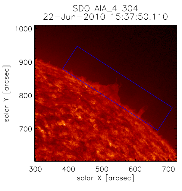
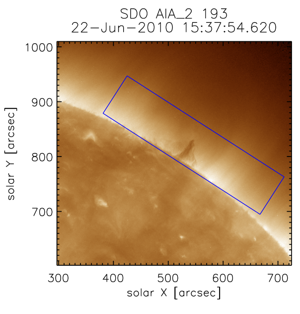
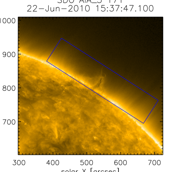
Figure 1: Prominence observations made by the AIA instrument are shown in its three wavelength channels: 304 Å (the left upper panel) dominated by the He II Lyman $\alpha$ line, 193 Å (the right upper panel) where mainly radiation of the Fe XII and Fe XXIV lines are detected and 171 Å (the lower panel) where the Fe IX and Fe X lines contribute. In the 304 Å channel image whole prominence is seen well in emission while in 193 Å and 171 Å images mainly its spine is seen as dark structure. Prominence barbs are seen in emission in the 171 Å channel due to the Fe IX line formed in PCTR.

Figure 2: The prominence observed as filament at 304 Å by the EUVI instrument on-board of the STEREO A satellite. The image was made close in time to XRT and AIA observations. Filament structures are faint and geometrically thin so much that area in which the filament occurs should be marked by white border. Nevertheless long spine on one end of the filament and two barbs on the other are well distinguishable.

XRT observed the corona at the prominence location and its vicinity in SXR using two of its focal-plane analysis filters Al-mesh and Ti-poly. XRT observations were made between 13:18:13 and 17:39:31 UT with exposure times from 4.1 up to 16.4 s. Field of view (FOV) of the observed images is $788$ arcsec $\times\,788$ arcsec and dimensions of one pixel is $2.06\,$ arcsec $\times\,2.06$ arcsec. The data were processed using standard data reduction routines in SolarSoft (Freeland & Handy, 1998) provided by the XRT team (Kobelski et al., 2014). Observations in the two filters made at 15:37:45 and 15:37:58 UT, respectively, are shown in Fig. 3. There is a time-dependent contamination layer on the CCD (see Narukage et al. 2011, 2014) and contamination spots which manifest as small dark areas in XRT observation images. Especially, the original Al-mesh image was studded with many such spots. In both images in Fig. 3, spots were retouched by an interpolation to see better the darkening occurring at the prominence spine. In the Al-mesh image in the left panel of the figure, dark radial structure (seen in the AIA 193 Å and 171 Å images) at spine is clearly visible, while in Ti-poly it is much weaker. Because the response of both filters to SXR is rather similar (peaked around 10 Å), an additional darkening in the Al-mesh image is most probably caused by a secondary peak in its transmittance function - we address this effect in the present paper.

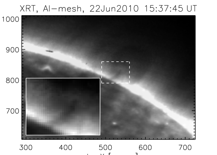
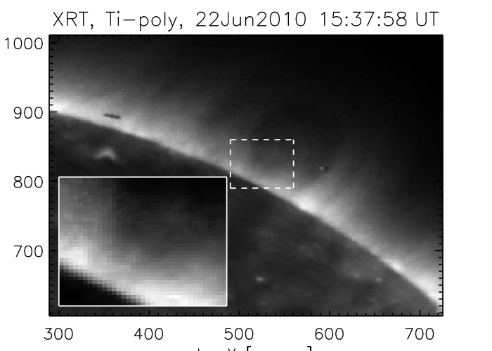
Figure 3: XRT images of the X-ray corona at place of the prominence and its vicinity made with the Al-mesh (the left panel) and Ti-poly (the right panel) focal-length filters made at 15:37 UT. Other Al-mesh and Ti-poly images of the prominence place made between 13:18:13 and 17:39:31 UT look similar as these two images.

3 Soft X-ray Visibility of Prominences

In order to investigate darkening in the SXR images in detail, we made cuts tangentially to the limb in both Al-mesh and Ti-poly images taken at 15:37:45 and 15:37:58 UT, respectively, at four different heights as shown in Fig. 4. Heights above the limb at which the cuts were made were chosen so that they would not intersect any contamination spot at least at places of the prominence location and its vicinity. Three cuts were made close to each other at heights 14 500, 17 000 and 19 500 km and the fourth one at a larger height of 31 000 km. Resulting intensity plots along cuts are shown in Fig. 5. A noticeable decrease in the intensity occurs at position of the prominence spine in Al-mesh filter in all four cuts. In Ti-poly along the four cuts a decrease also occurs at position of the dark prominence structure, but somewhat shallower than in the case of Al-mesh data.

There are two known mechanisms that can be responsible for the darkening: absorption of background coronal radiation by the cool prominence plasma and/or the so-called coronal emissivity deficit (formerly called volume or emissivity blocking). Although Anzer et al. (2007) already showed that there is a negligible amount of absorption in the hydrogen and helium prominence plasma at wavelengths around 50 Å  (they used the Yohkoh observations), we can expect some additional opacity due to metals around 10 Å  where both XRT filters have their peaks in the X-ray domain. Moreover, the line of sight crosses an extended volume occupied by a cool prominence plasma not emitting in SXR that can cause lower intensities in the corona – the coronal emissivity deficit.

However, the two filters we used have quite different responses to the EUV part of the spectrum. While the Ti-poly transmittance has mainly one peak around 10 Å, the Al-mesh filter has two transmittance maxima, one also around 10 Å  and the other one around 171 Å. This then means that apart from the absorption and emissivity deficit, a more pronounced darkening in Al-mesh can be explained by a contamination from the secondary EUV peak of the filter. In the following subsections we first estimate the total prominence opacity in the X-ray domain taking into account several important metals and then explain the darkening in Ti-poly alone. In the last subsection we show how the Al-mesh images are affected by the secondary EUV transmittance peak.

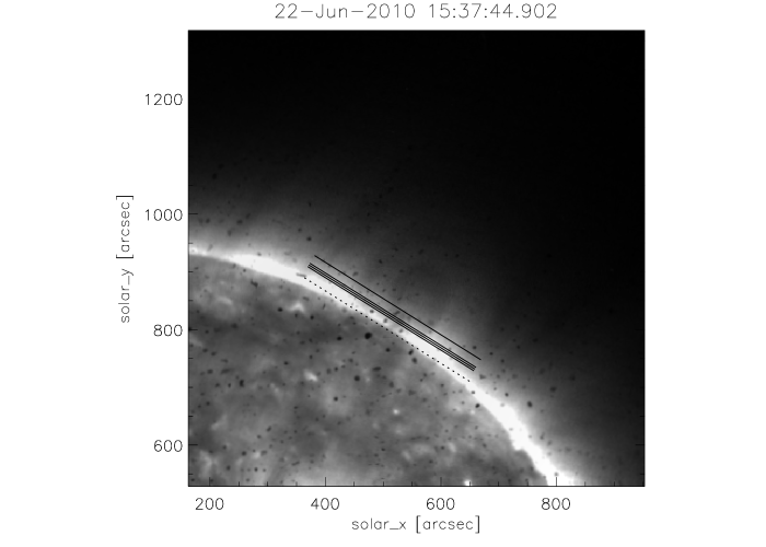
Figure 4: The original (before retouching the contamination spots) XRT Al-mesh image taken at 15:37 UT. Intensities along cuts made tangentially to limb in four heights are used for estimations of depth of depression at the place of prominence spine. The cuts are marked by black solid lines and tangent to the limb at the prominence spine by dashed black line. Cuts at the same heights were made also in the Ti-poly image taken almost 13 seconds later.

Figure 5: Intensity distributions along the four cuts made at heights 14 500, 17 000, 19 500 and 31 000 km above the limb in the Al-mesh and Ti-poly images taken at 15:37 UT. Depression at the prominence spine (positions along the cuts 110 000 – 120 000 km) is seen well in data from both filters in all four heights although it is much shallower in the Ti-poly data. For estimating of the quiet-corona intensity along each cut, an average value at positions around 50 000 km along the cut outside contamination spots was used.

4 Mechanisms of prominence SXR darkening

4.1 Soft X-ray absorption

The absorption of X-ray background coronal radiation is caused by hydrogen and helium resonance continua and by continua of some metals (the process called photoionisation). The cross sections and total optical thickness at resonance continua of hydrogen and helium mixture have been calculated by Anzer & Heinzel (2005) for cool gas located at the corona. Cross sections of neutral hydrogen and singly ionised helium at a given wavelength ($\lambda$) of the resonance continuum are proportional to $\lambda^{3}$

$$\sigma_{\mathrm{HI}}(\lambda)=\sigma_{0}\,g_{\mathrm{HI}}(\lambda)\,\left(\frac{\lambda}{912}\right)^{3}$$ (1)

and

$$\sigma_{\mathrm{HeII}}(\lambda)=16\,\sigma_{0}~{}g_{\mathrm{HeII}}(\lambda)\,\left(\frac{\lambda}{912}\right)^{3}\,,$$ (2)

where 912 presents the Lyman limit of the neutral hydrogen in units of Å. Here $\sigma_{0}=7.91\times 10^{-18}$ cm^-2, $g_{\rm HI}$ is the hydrogen Gaunt factor (see Karzas & Latter, 1961), and $g_{\mathrm{HeII}}(\lambda)=g_{\mathrm{HI}}(4\,\lambda)$. The cross section of neutral helium is obtained from Fig. 2 in Brown & Gould (1970).

The optical thickness of hydrogen and helium mixture at SXR spectral range (see Anzer & Heinzel 2005) is given by

$$\tau_{\mathrm{H+He}}(\lambda) = N_{\mathrm{H}}\,\left\{(1-i)\,\sigma_{\mathrm{HI}}(\lambda)+r_{\mathrm{He}}\,\left[(1-\right.\right.$$

$$\left.\left.-j_{1}-j_{2})\,\sigma_{\mathrm{HeI}}(\lambda)+j_{1}\,\sigma_{\mathrm{HeII}}(\lambda)\right]\right\}\,,$$

where $N_{\mathrm{H}}$ is the total hydrogen column density ($N_{\mathrm{H}}=N_{\mathrm{HI}}+N_{\mathrm{p}}$), $N_{\mathrm{HI}}$ and $N_{\mathrm{p}}$ are neutral hydrogen and proton column densities, respectively, $i$ is the ionisation degree of hydrogen defined as the ratio between the proton and total hydrogen column density, $r_{\mathrm{He}}$ is the abundance of the helium relative to hydrogen ($N_{\mathrm{He}}/N_{\mathrm{H}}$) and ionisation degrees of neutral and singly ionised helium $j_{1},j_{2}$, respectively, are defined as $j_{1}=N_{\mathrm{HeII}}/N_{\mathrm{He}}$ , $j_{2}=N_{\mathrm{HeIII}}/N_{\mathrm{He}}$ , where $N_{\mathrm{He}}=N_{\mathrm{HeI}}+N_{\mathrm{HeII}}+N_{\mathrm{HeIII}}$. For three typical values of $N_{\mathrm{H}}$ ($10^{17},10^{19},10^{21}\,\mathrm{cm}^{-2}$) taken from Gouttebroze et al. (1993), hydrogen and helium mixture with $r_{\mathrm{He}}$=0.1, $i$=0.3, $j_{1}$=0.3 and $j_{2}$=0, the optical thickness is calculated between 5 and 50 Å as shown in Fig. 6 (thin dashed lines for various $N_{\rm H}$).

X-ray absorption by hydrogen and helium at 50 Å was computed already by Anzer et al. (2007). Here we extend the wavelength range below 50 Å and add contributions of eight metal continua, i.e. C, N, O, Ne, Mg, Si, S, Fe. Photoionisation cross sections of these eight abundant metals are computed using an approximate formula which depends on the energy $E$ (see London et al., 1981)

$$\sigma(E)=\sigma_{\mathrm{T}}\left[a\,\left(\frac{E_{\mathrm{T}}}{E}\right)^{3}+(1-a)\,\left(\frac{E_{\mathrm{T}}}{E}\right)^{4}\right]\,.$$ (4)

Here $E_{\mathrm{T}}$ and $\sigma_{\mathrm{T}}$ are the threshold energy and threshold cross section, respectively, and $a$ is a parameter chosen to match the slope near the threshold (see Table 3 in London et al. 1981). Comparison of cross sections of metals between the approximate formula given by London et al. (1981) and Fig. 2 in Brown & Gould (1970), which is mostly cited in the literature, gives a difference of the order of 10 %. The best agreement is for Si (1 %) and the worst for S (21 %). Optical thickness of metals is expressed in the form

$$\tau_{\lambda}=N_{\mathrm{H}}\,\sum\limits_{i=1}^{8}\sigma_{i}(E)\,A_{i}\,,$$ (5)

where $A_{i}$ represents the abundance of a chosen metal marked by subscript $i$ given in Table 3 of London et al. (1981). Optical thickness is calculated for all eight abundant metal elements under the condition $E\geq E_{\mathrm{T}}$, otherwise $\sigma(E)$=0. Note that in our calculations we used the photospheric abundances of metals; the coronal abundances would lead to even smaller opacities. Note here that the metallic opacity is not sensitive to the ionisation degree of individual metals, because we are dealing here only with the inner-shell electrons (see also London et al. 1981).

Figure 6: Plot of the optical thickness due to metals as a function of wavelength marked with thin solid line. Lower set of curves is for $N_{\rm H}$=$10^{17}\,\mathrm{cm}^{-2}$, middle for $N_{\rm H}$=$10^{19}\,\mathrm{cm}^{-2}$ and upper for $N_{\rm H}$=$10^{21}\,\mathrm{cm}^{-2}$. From 5 Å  we also mark the optical thickness due to partially ionised hydrogen and helium mixture (with $r_{\rm He}$ = 0.1, $i$ = 0.3, $j_{1}$ = 0.3, $j_{2}$ = 0) marked with thin dashed line. The total contribution of hydrogen, helium and metals between 5 and 50 Å is marked by thick solid line.

Fig. 6 presents the optical thickness versus wavelength below 50 Å for three values of $N_{\mathrm{H}}$. Contribution of metals is marked with thin solid line. Small ”jumps” on the curves occur when metals stop to contribute above certain wavelength (their $E_{\mathrm{T}}$). The total contribution of hydrogen and helium mixture and of all metals is presented by thick solid lines. Above 20 Å the contribution of metals is negligible compared to hydrogen and helium mixture. It is well seen that total $\tau_{\lambda}$ (hydrogen, helium and metals all together) is practically negligible in the SXR domain.

From the amount of EUV coronal emission at wavelengths below 912 Å absorbed by the hydrogen and helium prominence plasma, Kucera et al. (1998) and Golub et al. (1999) found the hydrogen column density $10^{18}$ – $10^{19}$ $\mathrm{cm}^{-2}$ in quiescent prominences. The hydrogen column densities in the same range were estimated also by Schwartz et al. (2015) from observations of six quiescent prominences in EUV, SXR and H$\alpha$. Even if one considers a limiting value 10²¹  $\mathrm{cm}^{-2}$ which, for example, would correspond to hydrogen density 10¹¹ $\mathrm{cm}^{-3}$ and the prominence extension of 10⁵ km, the optical thickness around 10 Å (where both Al-mesh and Ti-poly filters have the maximum responsibility) is below 0.02. Therefore the absorption mechanism can not explain the observed darkening and we must turn our attention to the effect of emissivity deficit.

4.2 Emissivity Deficit

In EUV and SXR, the prominence will appear dark in the coronal line/continuum emitted at temperatures higher than 10⁶ K. We assume that this is due to the absorption and emissivity deficit, i.e.

$$I_{\mathrm{prom}}(\lambda)=I_{\mathrm{fg}}(\lambda)+I_{\mathrm{bg}}(\lambda)\,\exp\left(-\tau_{\lambda}\right)\,,$$ (6)

where $I_{\mathrm{fg}}(\lambda)$ and $I_{\mathrm{bg}}(\lambda)$ are intensities of the radiation emitted by the corona in front and beyond the prominence, respectively. Assuming the most simple case when these intensities are equal (symmetric corona), we can write

$$I_{\mathrm{prom}}(\lambda)=I_{\mathrm{c}}(\lambda)\,\left[1+\exp\left(-\tau_{\lambda}\right)\right]\,,$$ (7)

where $I_{\mathrm{c}}\equiv I_{\mathrm{fg}}=I_{\mathrm{bg}}$.

In this paper we express the prominence darkening in terms of the intensity ratio R which we define as

$$R=\frac{I_{\mathrm{prom}}}{I_{0}}\,,$$ (8)

where $I_{0}$ is the coronal intensity measured close to the prominence. In the case of a negligible absorption, $R=2I_{\rm c}/I_{0}$ which demonstrates the effect of emissivity deficit, i.e. the lack of hot coronal emission at the volume occupied by the cool prominence material - see below. Sometimes it is also useful to express the prominence darkening in terms of the contrast, which can be defined as $C=1-R$. $C$ is zero in the case of no prominence visibility. If there is a negligible absorption, $C=1-2I_{\rm c}/I_{0}$ and, on the other hand, for large $\tau$, $C=1-I_{\rm c}/I_{0}$. In case of $I_{\rm c}=I_{0}/2$ (no deficit effect) the latter will give $C=1/2$.

The coronal intensity $I_{\rm c}$ at the prominence location is obtained by integration of the coronal emissivity along the line of sight (LOS), from middle of the (symmetrical) cool structure positioned at the limb to coronal boundaries

$$I_{\mathrm{c}}(\lambda)=\int_{0}^{\infty}\,C_{\lambda}(n_{e},T)\,\frac{n(\mathrm{H})}{n_{\rm e}}\,n_{\rm e}^{2}\,dl\,,$$ (9)

where $l$ is the position along the LOS expressed as

$$l=\sqrt{r^{2}-\left(R_{\mathrm{Sun}}+h\right)^{2}}\,.$$ (10)

Here $r$ is radial position in the corona, $R_{\mathrm{Sun}}$ the solar radius and $h$ the height above the limb. $n_{\rm e}$ and $n_{\rm H}$ are the electron and hydrogen densities, respectively, $T$ is the kinetic temperature and $C_{\lambda}$ is the contribution function calculated using the statistical equilibrium and CHIANTI atomic database version 7 (Dere et al., 1997; Landi et al., 2012). For the ratio $n(\mathrm{H})/n_{\rm e}$ a common coronal value 0.83 is adopted. Distributions of the temperature and electron density with height above the solar surface in the quiet corona were taken from Lemaire (2011) and Saito et al. (1970), respectively. In Eq. (9) we first integrate from the middle of the cool prominence structure up to its boundary $D_{\mathrm{geom}}/2$ (where $D_{\mathrm{geom}}$ represents the total LOS extension of the prominence), this automatically accounts for the emissivity deficit because $C_{\lambda}$ is there essentially zero. From the coronal part we get actual $I_{\rm c}$. In the quiet corona outside the prominence, this integral gives simply $I_{0}/2$. Finally, the signal measured by XRT is calculated by the integration of $I(\lambda)$ multiplied by the filter response function $f(\lambda)$ over the wavelength range of the filter.

$$E=\int\,I(\lambda)\,f(\lambda)\,d\lambda\,,$$ (11)

where $I(\lambda)$ is either $I_{\rm prom}$, $I_{\rm c}$ or $I_{0}$. Response functions $f(\lambda)$ for both Al-mesh and Ti-poly filters are shown in plots in Fig. 7.

Length 1.8$\times 10^{5}$ km of the prominence spine in projection on the solar disc was measured in image Fig. 2 made at 304 Å with the EUVI instrument onboard the STEREO A which observed the prominence as filament. But real length of the spine can be larger. Moreover, it can be possible for the prominence on-limb observations that the line of sight was not passing along whole length of the spine or part of the spine could be hiden behind the limb. Therefore, length estimated according to STEREO A observations cannot be used as $D_{\mathrm{geom}}$. For correct derivation of $D_{\mathrm{geom}}$ view from minimum three angles is necessary and only two are available (edge-on viewed from Earth direction and from above). Unfortunately, STEREO B was positioned by 75 $\deg$ from Earth in opposite direction than STEREO A and therefore the whole prominence was behind the limb for STEREO B. Thus, we used Ti-poly observations to estimate $D_{\mathrm{geom}}$ at four heights where the cuts have been made. $D_{\mathrm{geom}}$ was optimized in order to achieve the best fit between the observed and computed ratio $R$. Note that in the case of Ti-poly filter, the latter is equal to $2E_{\rm c}/E_{0}$ because the absorption at 10 Å is considered to be quite negligible and contribution of EUV radiation to measured signal is under 1 %. The resulting $D_{\mathrm{geom}}$ are shown in Table 1 and is used in the next subsection to evaluate the darkening in the Al-mesh images where the filter has a secondary peak in EUV which contributes to the integral in Eq. (11). All resulting values of $D_{\mathrm{geom}}$ are of order of magnitude of $10^{5}$ km that is close to length of the spine measured in EUVI image (Fig. 2) from the STEREO A satellite. But it has to be also noted that any of them do not exceed the spine length as measured in the STEREO A image.

Table 1: Comparison of observed and calculated intensity ratios ($R$) at the prominence spine for the Al-mesh and Ti-poly filters.

$h$	$R$ from observations		$D_{\mathrm{geom}}$	maximum $\tau_{193}$	$R$ from calculations
$\left[\mathrm{km}\right]$	Ti-poly	Al-mesh	$\left[10^{4}\,\mathrm{km}\right]$		Ti-poly	Al-mesh
14 500	0.83	0.77	$\ 7.8$	2.01	0.83	0.80
17 000	0.82	0.79	$\ 8.3$	2.67	0.82	0.79
19 500	0.81	0.76	$\ 8.9$	2.13	0.81	0.78
31 000	0.78	0.78	$10.0$	1.40	0.78	0.76

4.3 EUV Contribution from the Al-mesh Secondary EUV Peak

To evaluate the intensity ratio $R$ in the case of Al-mesh filter, we proceed in the same way as in previous subsection. The only difference is that we can not neglect the absorption because in the EUV domain around 170 Å, where the secondary peak of the Al-mesh filter contributes to the measured signal (see Fig. 7), the absorption of coronal radiation by cool hydrogen and helium prominence plasma can be significant. Although response for the Al-mesh filter around 170 Å is almost three orders of magnitude lower than at 10 Å, as shown in Fig. 7, the quiet corona in EUV around 170 Å is approximately $40$ times as intensive as its X-ray radiation at 10 Å. Thus, contribution from EUV to signal measured using the Al-mesh filter at the quiet corona cannot be neglected. And subsequently, decrease of this contribution due to the absorption at the prominence can have remarkable impact on the intensity ratio $R$. The map of the optical thickness $\tau_{193}$ at 193 Å of the prominence studied here has been already calculated by Gunár et al. (2014) using the SDO/AIA observations in the 193 Å channel (upper right panel of Fig. 1), SXR data from XRT (Fig. 4) and the method of Schwartz et al. (2015). Because of the assumption of symmetrical distribution of the coronal emissivity, factor of the coronal asymmetry $\alpha$ equal to 0.5 was used. The $\tau_{193}$ map is shown in Fig. 8. Position and shape of an area with $\tau_{193}$ above 2 corresponds well to the dark radial structure of prominence visible in the AIA 193 Å and XRT Al-mesh images. Thus, the minimal $R$ of the XRT data for both filters corresponds well with the maximum $\tau_{193}$ at all heights above the limb. They can be transformed to other wavelengths by multiplying with the $\tau_{\mathrm{H+He}}(193\,\mathrm{\AA})/\tau_{193}$ ratio obtained from Eq. (LABEL:eq:tauhhe) for estimation of the theoretical optical thickness of hydrogen and helium plasma $\tau_{\mathrm{H+He}}(193\,\mathrm{\AA})$, see e.g. Anzer & Heinzel (2005). In calculations of $\tau_{\mathrm{H+He}}(193\,\mathrm{\AA})$ in wavelength range from 1 to 300 Å (from X rays up to EUV) we adopted the same values of helium abundance and ionisation degrees ($r_{\mathrm{He}}$=0.1, $i$=0.3, $j_{1}$=0.3 and $j_{2}$=0) as in section 4.1. Resulting ratio is plotted in Fig. 9. Maximum values of $\tau_{193}$ occurring at the prominence spine are within an interval 1.4 – 2.7 for heights 14 500 – 31 000 km what corresponds to optical thickness at wavelengths around 170 Å of approximately 0.8 – 2.2. Such an optical thickness produces remarkable decrease of intensity and subsequently smaller EUV contribution (only 7 – 8 %) to signal measured at the prominence spine using the Al-mesh filter than for the quiet corona (the contribution of 11 % at heights 14 500 – 19 500 km, 9 % at the height 31 000 km). Then again the signal $E_{\mathrm{prom}}$ registered at the prominence by the Al-mesh filter is calculated by integration along the wavelength of $I_{\mathrm{prom}}(\lambda)$ multiplied by the instrument response $f(\lambda)$ (see Fig. 7), similarly as in the case of Ti-poly. Finally, the theoretical intensity ratio $R=E_{\mathrm{prom}}/E_{\mathrm{0}}$ at the prominence position is calculated. Note that the emissivity deficit is properly accounted for by using the values of $D_{\mathrm{geom}}$ obtained in the previous subsection.

For Al-mesh filter we compare the observed values of $R$ with those calculated assuming the EUV contamination in Table 1. For values of $D_{\mathrm{geom}}$ of the order of $10^{5}$ km and maximal $\tau_{193}$ between 1.4 and 2.67 a good agreement between calculated and observed values of $R$ was achieved for the four selected heights above the limb - see Table 1..

Figure 7: Intensities of the quiet corona within interval of wavelengths 1 – 300 Å calculated using Eq. (9) for height 14 500 km above the limb. Plotted intensities are mean values of spectral intensities within 20 Å interval bins. Al-mesh (left panel) and Ti-poly (right panel) filter responses are also plotted. Although the response in EUV peak at 170 Å is almost thousand times lower than for X rays at 10 Å for Al-mesh, intensities around 170 Å are approximately $40$ times as large as those at 10 Å. Thus, contribution of the EUV radiation from wavelengths around 170 Å to the measured signal is around 11 % that cannot be neglected. Similar EUV contribution was calculated for the quiet corona also at heights 17 000 and 19 500 km while at height 31 000 km the contribution was only 9 %. In the other hand, the response at 170 Å for the Ti-poly filter is four orders of magnitude lower than at 10 Å, thus EUV contribution to the measured signal is under 1 %.

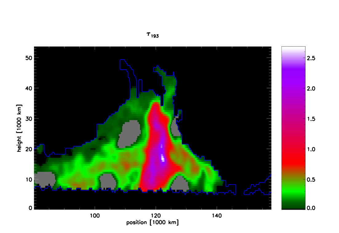
Figure 8: Map of the $\tau_{193}$ optical thickness obtained by Gunár et al. (2014) from amount of radiation from behind the same prominence in resonance continua of hydrogen and helium assuming symmetrical distribution of coronal emissivity along the line of sight. For calculations the method of Schwartz et al. (2015) and AIA 193 Å and XRT Al-mesh data shown in Figs 1 and 4, respectively, were used. Gray areas mark positions of contamination spots in the Al-mesh image where the data are corrupted.

Figure 9: The $\tau_{\mathrm{H+He}}(\lambda)/\tau_{193}$ ratio plotted within wavelength range 1 – 300 Å (from hard X rays up to EUV). Values of the optical thickness $\tau_{\mathrm{H+He}}(\lambda)$ were computed using the theoretical formula Eq, (LABEL:eq:tauhhe) for $\tau_{\mathrm{H+He}}(\lambda)$ calculation for the common solar helium abundance of $0.1$ and ionisation degrees of helium and hydrogen $i$=0.3, $j_{1}$=0.3 and $j_{2}$=0.

5 Discussion and Conclusions

In this paper we studied SXR visibility of the prominence observed on 22 June 2010 during the coordinated campaign. We noticed that a dark structure resembling the prominence spine is well visible in Hinode/XRT images obtained with Al-mesh and Ti-poly filters. Positions of the dark structure at all heights above the limb correspond to the maximal $\tau_{193}$ as estimated by Gunár et al. (2014) for the same prominence. We examined three possible mechanisms of SXR prominence darkening: absorption of X rays around 10 Å by the resonance continua of hydrogen, helium and selected metals, influence of the coronal emissivity deficit and the effect of a contamination by the secondary EUV peak in the case of the Al-mesh filter.

Comparison was made for four heights above the limb – three close to each other cutting the prominence spine somewhere in the middle between its bottom (at the limb) and top and the fourth close to its top. For the theoretical calculations, distributions of electron densities and temperature in the quiet corona were used and for the absorption of EUV radiation by hydrogen and helium plasma, maximal $\tau_{193}$ values for the four heights calculated for this prominence by Gunár et al. (2014) were scaled. Then, calculated intensities were integrated along wavelength using the XRT filter responses in order to obtain signal that should be measured by the XRT instrument.

We found that both absorption in resonance continua of hydrogen and helium of EUV radiation that contaminates SXR data and EUV emissivity deficit would lower $R$ at the prominence spine when using the Al-mesh filter. In case of the Ti-poly filter, lowering of $R$ due to absorption of EUV radiation is negligible.

As for absorption of X-ray radiation by prominence hydrogen and helium plasma, it is totally negligible at 10 Å. But when also continua of other elements (metals) such as C, N, O, Ne, Mg, Si, S, and Fe are taken into account, total optical thickness cannot be neglected for hydrogen column density exceeding $10^{21}\,\mathrm{cm}^{-2}$. For the prominence studied here we estimated the hydrogen column density at hydrogen and helium ionisation degrees $i$=0.6, $j_{1}$=0.5 and $j_{2}$=0 from the $\tau_{193}$ map constructed by Gunár et al. (2014) and we found a maximum column density of hydrogen being of $2\times 10^{19}\,\mathrm{cm}^{-2}$ for this prominence. It means that absorption of X rays at 10 Å can be neglected for the prominence studied here. Only when assuming that the line of sight at the prominence location is passing through a volume occupied by the cool prominence plasma not emitting in EUV and X-rays, the contrast comparable to observations is achieved due to the coronal emissivity deficit. For simplicity position of the prominence exactly at the limb was assumed. For the geometrical thickness $D_{\mathrm{geom}}$ of the prominence spine along the line of sight of the order of $10^{5}\,\mathrm{km}$, calculated intensity ratios comparable to those obtained from observations were obtained for all four selected heights (Table 1) for both Al-mesh and Ti-poly filters. Although $D_{\mathrm{geom}}$ is increasing with height, its variations are not exceeding 20 %. Thus, it can be just due to noise in the XRT Ti-poly data. But increase of $D_{\mathrm{geom}}$ with height could be also a real effect of the prominence shape. Unfortunately, observations of the prominence only in two viewing angles are available – edge-on on the limb and viewed as a filament projected on the disk from STEREO A. Therefore it is not possible to infer reliably its 3D shape and subsequently geometrical thickness of the prominence at the four heights. Thus, it is not possible to distinguish whether increase of $D_{\mathrm{geom}}$ with height is caused by noise in the data or by shape of the prominence. Although, such behaviour of the geometrical thickness might conform a loop-like shape of the prominence where at smaller heights the line of sight is passing through its vertical parts while in larger heights the line of sight is passing along its horizontal part. In case of the the Al-mesh filter also the EUV transmittance peak that contaminates the measured signal was taken into account. Calculated EUV contribution to the signal in case of the Al-mesh filter for the quiet corona is 11 % at heights 14500–19500 km. The EUV contribution at the prominence spine is 7–8 % in all four heights. This difference in EUV contributions causes decrease of measured XRT signal at the prominence spine together with the emissivity deficit. Comparing contribution to the signal from quiet-Sun radiation in X rays (main peak of the Al-mesh filter transmittance within wavelength interval 1 – 30 Å) and EUV (secondary peak at 160 – 210 Å) it was found that contribution of EUV to depression of measured signal in the quiet corona decreases steeply with height. At the height of 31 000 km the EUV contribution to the signal in the quiet corona is lower – only 9 % while at the prominence spine the contribution is the same as at lower heights. Thus, lower EUV contribution to the measured signal in the quiet corona at $h$=31 000 km causes notably less dramatic intensity decrease at the prominence for this height than at lower heights as can be seen in Fig. 5. Although mainly the coronal emissivity deficit is responsible for visibility of this prominence in XRT images, in case of the Al-mesh filter a fraction of 16 – 25 % of the total darkening comes from the EUV contamination. Therefore depression of the measured signal at the prominence in case of the Al-mesh filter is more prominent and its variations with height are larger than in case of the Ti-poly filter. In contrast, the contamination of Ti-poly signal by the EUV radiation is negligible and thus the emissivity deficit only causes depression at the prominence spine in XRT observations made with the Ti-poly filter.

References

- Anzer & Heinzel (2005) Anzer, U. & Heinzel, P. 2005, ApJ, 622, 714
- Anzer et al. (2007) Anzer, U., Heinzel, P., & Fárnik, F. 2007, Sol. Phys., 242, 43
- Berlicki & Heinzel (2004) Berlicki, A. & Heinzel, P. 2004, A&A, 420, 319
- Brown & Gould (1970) Brown, R. L. & Gould, R. J. 1970, Phys. Rev. D, 1, 2252
- Culhane et al. (2007) Culhane, J. L., Harra, L. K., James, A. M., et al. 2007, Sol. Phys., 243, 19
- Delaboudinière et al. (1995) Delaboudinière, J.-P., Artzner, G. E., Brunaud, J., et al. 1995, Sol. Phys., 162, 291
- Dere et al. (1997) Dere, K. P., Landi, E., Mason, H. E., Monsignori Fossi, B. C., & Young, P. R. 1997, A&AS, 125, 149
- Driesman et al. (2008) Driesman, A., Hynes, S., & Cancro, G. 2008, Space Sci. Rev., 136, 17
- Freeland & Handy (1998) Freeland, S. L. & Handy, B. N. 1998, Sol. Phys., 182, 497
- Golub et al. (1999) Golub, L., Bookbinder, J., Deluca, E., et al. 1999, Physics of Plasmas, 6, 2205
- Golub et al. (2007) Golub, L., Deluca, E., Austin, G., et al. 2007, Sol. Phys., 243, 63
- Gouttebroze et al. (1993) Gouttebroze, P., Heinzel, P., & Vial, J. C. 1993, A&AS, 99, 513
- Gunár et al. (2014) Gunár, S., Schwartz, P., Dudík, J., et al. 2014, A&A, 567, A123
- Hawley & Fisher (1992) Hawley, S. L. & Fisher, G. H. 1992, ApJS, 78, 565
- Heinzel et al. (2008) Heinzel, P., Schmieder, B., Fárník, F., et al. 2008, ApJ, 686, 1383
- Henoux & Nakagawa (1977) Henoux, C. & Nakagawa, Y. 1977, A&A, 57, 105
- Karzas & Latter (1961) Karzas, W. J. & Latter, R. 1961, ApJS, 6, 167
- Kobelski et al. (2014) Kobelski, A. R., Saar, S. H., Weber, M. A., McKenzie, D. E., & Reeves, K. K. 2014, Sol. Phys., 289, 2781
- Kosugi et al. (2007) Kosugi, T., Matsuzaki, K., Sakao, T., et al. 2007, Sol. Phys., 243, 3
- Kucera et al. (1998) Kucera, T. A., Andretta, V., & Poland, A. I. 1998, Sol. Phys., 183, 107
- Landi et al. (2012) Landi, E., Del Zanna, G., Young, P. R., Dere, K. P., & Mason, H. E. 2012, ApJ, 744, 99
- Lemaire (2011) Lemaire, J. F. 2011, ArXiv e-prints
- Lemen et al. (2012) Lemen, J. R., Title, A. M., Akin, D. J., et al. 2012, Sol. Phys., 275, 17
- London et al. (1981) London, R., McCray, R., & Auer, L. H. 1981, ApJ, 243, 970
- Narukage et al. (2011) Narukage, N., Sakao, T., Kano, R., et al. 2011, Sol. Phys., 269, 169
- Narukage et al. (2014) Narukage, N., Sakao, T., Kano, R., et al. 2014, Sol. Phys., 289, 1029
- Parenti et al. (2012) Parenti, S., Schmieder, B., Heinzel, P., & Golub, L. 2012, ApJ, 754, 66
- Saito et al. (1970) Saito, K., Makita, M., Nishi, K., & Hata, S. 1970, Annals of the Tokyo Astronomical Observatory, 12, 53
- Schwartz et al. (2015) Schwartz, P., Heinzel, P., Kotrč, P., et al. 2015, A&A, 574, A62
- Suematsu et al. (2008) Suematsu, Y., Tsuneta, S., Ichimoto, K., et al. 2008, Sol. Phys., 249, 197
- Tsuneta et al. (1991) Tsuneta, S., Acton, L., Bruner, M., et al. 1991, Sol. Phys., 136, 37
- Wuelser et al. (2004) Wuelser, J.-P., Lemen, J. R., Tarbell, T. D., et al. 2004, in Society of Photo-Optical Instrumentation Engineers (SPIE) Conference Series, Vol. 5171, Telescopes and Instrumentation for Solar Astrophysics, ed. S. Fineschi & M. A. Gummin, 111–122