Multiplicative logarithmic corrections to quantum criticality
in three-dimensional dimerized antiferromagnets

Abstract

We investigate the quantum phase transition in an $S=1/2$ dimerized Heisenberg antiferromagnet in three spatial dimensions. By performing large-scale quantum Monte Carlo simulations and detailed finite-size scaling analyses, we obtain high-precision results for the quantum critical properties at the transition from the magnetically disordered dimer-singlet phase to the antiferromagnetically ordered Néel phase. This transition breaks O($N$) symmetry with $N=3$ in $D=3+1$ dimensions. This is the upper critical dimension, where multiplicative logarithmic corrections to the leading mean-field critical properties are expected; we extract these corrections, establishing their precise forms for both the zero-temperature staggered magnetization, $m_{s}$, and the Néel temperature, $T_{N}$. We present a scaling Ansatz for $T_{N}$, including logarithmic corrections, which agrees with our data and indicates exact linearity with $m_{s}$, implying a complete decoupling of quantum and thermal fluctuation effects even arbitrarily close to the quantum critical point. We also demonstrate the predicted $N$-independent leading and subleading logarithmic corrections in the size-dependence of the staggered magnetic susceptibility. These logarithmic scaling forms have not previously been identified or verified by unbiased numerical methods and we discuss their relevance to experimental studies of dimerized quantum antiferromagnets such as TlCuCl₃.

I Introduction

Antiferromagnetic insulators exhibit a multitude of fundamental phenomena in the neighborhood of the phase transitions separating their magnetically ordered ground states from different types of quantum paramagnetic phase. These quantum phase transitions (QPTs) occur at temperature $T=0$ as a consequence of non-thermal parameters (examples include magnetic fields, applied pressure, and dopant concentration) that act to change the effect of quantum mechanical fluctuations Sachdev2008 ; Kaul2013 . At finite temperatures, a further dimension is opened in the presence of both quantum and classical (thermal) fluctuations, and the rich physics arising from their interplay includes all the properties of the quantum critical (QC) regime rs .

Experimentally, the material in which the most detailed study of intertwined classical and quantum critical behavior has been performed is TlCuCl₃. This compound is composed of antiferromagnetically coupled pairs of Cu²⁺ ions ($S=1/2$), which tend to form dimer singlets and have antiferromagnetic interdimer couplings in all three spatial dimensions ($d=3$) Matsumoto2004 . At ambient pressure and zero field, TlCuCl₃ is a nonmagnetic insulator with a gap of 0.63 meV to triplet spin excitations. As a consequence of this small gap, an applied magnetic field of 5.4 T is sufficient to drive the system to an ordered antiferromagnetic state, through a QPT in the Bose-Einstein universality class rgrt . A relatively small applied hydrostatic pressure, $p_{c}=1.07$ kbar, is also sufficient to create an antiferromagnetically ordered state rrs2004 , through a QPT in the three-dimensional (3D) O(3) universality class due to spontaneous breaking of the SU(2) spin symmetry (which is further reduced in TlCuCl₃ by a weak unixial anisotropy, making the universality class 3D XY).

The elementary excitations on the ordered side of the zero-field quantum critical point (QCP) are gapless spin waves, the Goldstone modes associated with spontaneous breaking of spin-rotational symmetry. On the disordered side, quantum fluctuations, towards spin-singlet formation on the dimers, suppress the long-range antiferromagnetic order, restoring the symmetry and ensuring that all excitations are gapped. This evolution of the excitation spectrum in TlCuCl₃ has been measured in Ref. Ruegg2008 . At finite temperatures on the ordered side, a classical phase transition occurs at the Néel temperature, $T_{N}$, where the long-ranged magnetic order is “melted” not by quantum but by thermal fluctuations. At finite temperatures around the QCP, the combination of quantum and thermal fluctuations creates the QC regime, where the only characteristic energy scale of the system is the temperature itself and many universal properties emerge rs . The phase diagram of TlCuCl₃ under pressure and the restoration of classical critical scaling around $T_{N}$ were the subject of a recent investigation Merchant2014 .

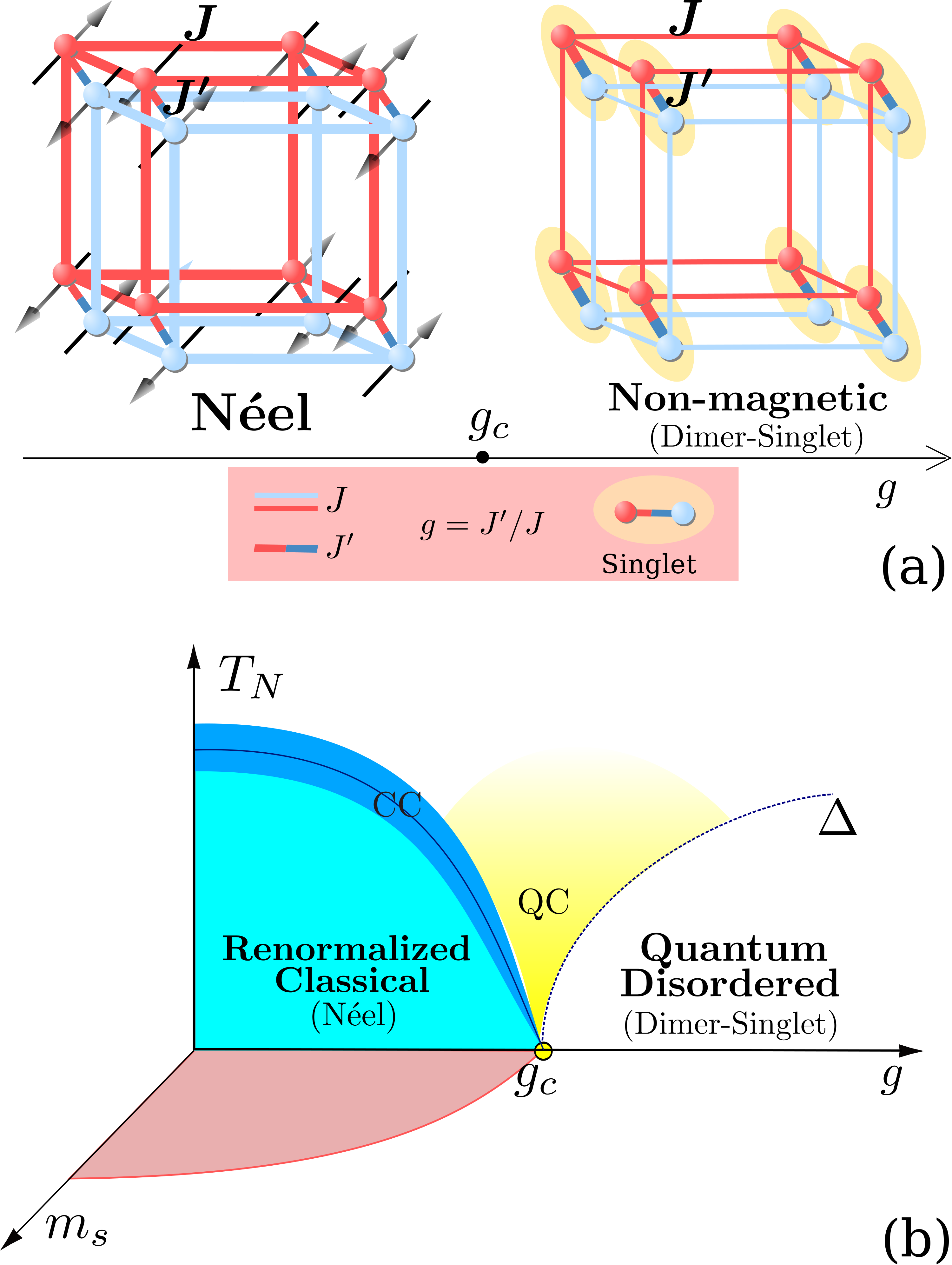
Figure 1: (Color online) (a) Dimerized lattice of $S=1/2$ spins in the 3D double cubic geometry. Sites of the red and blue cubic lattices are connected pairwise by dimer bonds; $J^{\prime}$ and $J$ are antiferromagnetic Heisenberg interactions, respectively on and between the dimer units, and their ratio, $g=J^{\prime}/J$, controls the QPT from a Néel ordered phase (left) to a quantum disordered dimer-singlet phase (right), with the QCP occurring at the critical ratio $g_{c}$. (b) Schematic quantum critical phase diagram for the Heisenberg model on the double cubic lattice. On the ordered “renormalized classical” side, $g<g_{c}$, the Néel order is progressively weakened by increasing quantum fluctuations as $g$ approaches $g_{c}$, causing both the ordering (Néel) temperature, $T_{N}(g)$, and the order parameter (the staggered magnetization), $m_{s}(g)$, to go continuously to zero. On the “quantum disordered” side, intradimer correlations dominate and the characteristic energy scale, $\Delta$, is the gap to triplet excitations. Above $g_{c}$ at $T>0$ is the universal “quantum critical” (QC) region, whose behavior is governed by the $3+1$-dimensional O(3) universality class. Around $T_{N}(g)$, one expects a region of classical critical (CC) behavior where thermal fluctuations are dominant.

QPTs in dimerized quantum spin models have been studied numerically by a number of authors, primarily by quantum Monte Carlo (QMC) simulations. Early investigations of the bilayer square-lattice antiferromagnet Sandvik1994 and other two-dimensional geometries Troyer1996 ; Matsumoto2001 have been followed more recently by high-precision studies of a range of critical properties Wang2006 ; Meng2008 ; Wenzel2009 ; Sandvik2010 ; Sen2015 . In three dimensions, the focus of investigations has been on the field-induced transition Nohadani2005 , on the effects of dimensionality Troyer1997 ; Yao2007 , and on physical observables at the coupling-induced QPT Jin2012 ; Oitmaa2012 ; Kao2013 .

A minimal model of a dimerized quantum antiferromagnet has only two coupling constants, $J^{\prime}$ on and $J$ between the dimer units, and therefore only one control parameter, $g=J^{\prime}/J$. The geometry considered in the present study is the double cubic lattice shown in Fig. 1(a). In this system at large $g$, intradimer singlet correlations dominate the physics and the ground state is magnetically disordered, while at small $g$ the interdimer correlations establish long-ranged magnetic order. The order parameter of the Néel phase is the staggered magnetization, $m_{s}(g)$, and along with the ordering temperature, $T_{N}(g)$, it can be driven continuously to zero by increasing $g$, as illustrated in Fig. 1(b). By standard arguments of dimensionality and symmetry, the dynamical exponent of this system is $z=1$ rs ; Chakravarty88 and the QCP belongs to the $D=3+1$ O(3) universality class, which is at the upper critical dimension, $D_{c}=4$, of all O($N$) models Zinn-Justin2002 ; rs . At $D=D_{c}$, mean-field critical scaling behavior alone is not sufficient to capture the physics of fluctuations around the QCP and multiplicative logarithmic corrections to the physical quantities (thermodynamic functions) are expected.

The theoretical importance of multiplicative logarithmic corrections to mean-field scaling behavior lies not only in the statistical physics of condensed matter systems but also in high-energy physics Zinn-Justin2002 ; rkbc . The general problem of a quantum field theory with an $N$-component field is encapsulated by an “O($N$) $\phi^{4}$ theory,” a Lagrangian containing a dynamic (quadratic gradient) term and a potential term with quadratic ($\phi^{2}$) and quartic ($\phi^{4}$) contributions. On changing the sign of the quadratic term, the system is driven through a QPT separating a phase with $\langle\phi\rangle=0$ from one with $\langle\phi\rangle\neq 0$ (a “Mexican hat” potential). As noted above, the low-energy properties of the 3D dimerized antiferromagnet of SU($2$) quantum spins with Heisenberg interactions correspond to a field theory with $N=3$ and $D=3+1$ (including the time dimension); $N=1$ and $2$ correspond respectively to Ising and XY spin interactions.

Beyond the upper critical dimension $(D>D_{c})$, the scaling behavior of the O($N$) $\phi^{4}$ theory is straightforward, with the critical exponents being exactly those given by mean-field theory Aizenman1981 ; rbg ; rkbc , namely $\alpha=0$, $\beta={1}/{2}$, $\gamma=1$, $\delta=3$, and $\nu={1}/{2}$. As we discuss below, this may be taken as an expression of the independence of quantum and thermal fluctuations when the phase space is sufficiently large. For $D<D_{c}$, the situation is complex and these exponents take anomalous values. However, exactly at the upper critical dimension, $D=D_{c}=4$, the leading scaling behavior coincides with that of the mean-field theory, but modified by multiplicative logarithmic corrections rkl ; rkle ; Zinn-Justin2002 . While the leading exponents are $N$-independent, a measure of $N$-dependence resides in the logarithmic corrections and these must be taken into account to establish the universality class of the transition Janssen2004 . Because the established results for the form of these corrections are based on perturbative techniques applied to low-energy theories, it is desirable to verify them using unbiased numerical methods applied directly to the lattice Hamiltonians, and this is what we achieve here.

Despite the insight into general QPT phenomena obtained from simulations using this type of minimal model for 3D dimerized systems Nohadani2005 ; Troyer1996 ; Yao2007 ; Jin2012 ; Oitmaa2012 , the question of logarthmic corrections has to date been addressed only briefly and inconclusively tbk07 ; Kao2013 . Experimentally, the feasibility of observing logarithmic corrections in systems such as TlCuCl₃ remains a challenging open issue Merchant2014 . In this paper we provide a systematic numerical study. We employ large-scale QMC simulations to investigate the critical behavior of the order parameter and Néel temperature on the double cubic lattice [Fig. 1(a)] for small values of $|g-g_{c}|$ unattainable in all previous studies. State-of-the-art QMC techniques and finite-size-scaling analysis using very large systems (sizes exceeding $10^{5}$ spins) allow us to detect and characterize the multiplicative logarithmic corrections in the universal scaling relations for the QC regime at the upper critical dimension, here for the $D=3+1$ O(3) QCP. In fact our results constitute hitherto unavailable exact numerical verification of the logarithmic forms predicted both by perturbative renormalization-group calculations rw ; rwr ; rblzj based on the $N$-component $\phi^{4}$ theory at $D_{c}$ and by additional considerations exploiting the zeros of the partition function rkl ; rkle ; Kenna2004 ; rkbc . To the best of our knowledge, no systematic numerical calculations have been performed beyond $N=1$ rkl ; rfkp .

As will become clear, our numerical results demonstrate to high precision the validity of the detailed theoretical predictions for the expected universality class. Both size-dependent scaling and the order parameter in the thermodynamic limit show evident deviations from pure mean-field behavior, which are accounted for by logarithmic corrections whose exponents are in very close ageement with the predicted values where available. In the case of the Néel temperature, we are not aware of any previous scaling predictions including logarithms. Here we test an Ansatz based on the known scaling behavior for the relevant energy scales rs ; Fisher1989 and the logarithmic corrections in corresponding classical systems rkbc . In addition to probing the asymptotic behavior, our results also provide direct insight into the range of validity of logarithmically modified critical scaling forms as one moves away from the QCP, which will be essential in evaluating the experimental relevance of logarithmic corrections.

The paper is organized as follows. In Sec. II we introduce the model and the numerical method, describing the measurement of physical observables in our QMC simulations. In Sec. III we begin the presentation of our numerical results with the precise determination of $g_{c}$, the position of the QCP, using finite-size-scaling techniques. Section IV discusses the observation of clear logarithmic corrections in the staggered magnetic susceptibility, ${\chi}(\mathbf{Q}_{\rm AF},L)$, at the QCP as a function of the system size, $L$. We present our results for the sublattice magnetization, $m_{s}$, at $T=0$ in Sec. V, discussing in detail its extrapolation to the thermodynamic limit, where we investigate the presence of logarithmic corrections to the leading mean-field behavior. In Sec. VI we present a scaling Ansatz for the Néel temperature, apply finite-size scaling to extract it as a function of $g$, and again investigate corrections to mean-field behavior. We compute the characteristic velocity $c$ of spin excitations, demonstrate the precise linearity of $T_{N}$ and $m_{s}$, and discuss the physical interpretation of this behavior. We summarize our results in Sec. VII and comment further on their theoretical and experimental consequences.

II Model and methods

As a representative 3D dimerized lattice with an unfrustrated geometry, we choose to study the double cubic model shown in Fig. 1(a). This system consists of two interpenetrating cubic lattices with the same antiferromagnetic interaction strength, $J$, connected pairwise by another antiferromagnetic interaction, $J^{\prime}$. The QPT occurs when the coupling ratio $g=J^{\prime}/J$ is increased, changing the ground state from a Néel-ordered phase of finite staggered magnetization to a dimer-singlet (“quantum disordered”) phase, as illustrated in Fig. 1(b). An advantage of this geometry over cases where the dimerization is imposed within a single lattice, such as the simple cubic lattice Jin2012 , is that all symmetries of the cubic lattices are retained, facilitating the consideration of quantities such as the spin stiffness or the velocity of spin excitations.

The Hamiltonian is given by

$$H=\sum_{\langle i,j\rangle}J_{ij}{\vec{S}}_{i}\cdot{\vec{S}}_{j},$$ (1)

where ${\vec{S}}_{i}$ is an $S=1/2$ spin operator residing on a double cubic lattice of $N=2L^{3}$ sites with periodic boundary conditions. The sum is taken only over nearest-neighbor sites, where every site has six neighbors on the same cubic lattice with coupling strength $J_{ij}=J$ and one neighbor on the opposite cubic lattice with $J_{ij}=J^{\prime}$ [Fig. 1(a)]. We set $J=1$ as the unit of energy and use $g=J^{\prime}/J$ as the control parameter.

To study this system, we use the stochastic series expansion (SSE) QMC technique Sandvik1991 ; Sandvik1999 ; Evertz2003 ; Sandvik2010 to obtain unbiased results, i.e. numerically exact within well-characterized statistical errors, for physical quantities in systems of finite side-length $L$. Here we present results up to $L=48$ at temperatures $T=\beta^{-1}$ with $\beta$ up to $2L$. We then perform detailed analyses by finite-size scaling Fisher1972 to extract information in the thermodynamic limit both in the ordered state and at the QCP, as detailed in the separate sections to follow. Here we define the physical quantities of interest and discuss some technical aspects of their calculation within the SSE QMC method.

Because spin-rotation symmetry is not broken in simulations of finite-size systems, one may measure the squared order parameter and take its square root as a post-simulation step. The staggered magnetization is given by

$$m_{s}=\sqrt{\frac{1}{N}S(\mathbf{Q}_{\rm AF})},$$ (2)

where

$$S(\mathbf{q})=\frac{1}{N}\sum_{i,j}^{N}e^{-i\mathbf{q}\cdot(\mathbf{r}_{i}-\mathbf{r}_{j})}\langle\vec{S}_{i}\cdot\vec{S}_{j}\rangle$$ (3)

is the magnetic structure factor, with $\mathbf{r}_{i}$ denoting the real-space position of the spin $\vec{S}_{i}$ on lattice site $i$, and $\mathbf{Q}_{\rm AF}=(\pi,\pi,\pi,\pi)$ is the wave vector of antiferromagnetic order, with the fourth $\pi$ denoting the phase factor between the two cubic lattices. We consider only the $z$-component of the magnetization and average it over the time dimension of the QMC configurations, computing the expectation value of the squared order parameter in the form

$$m^{2}_{sz}=\frac{1}{\beta}\int^{\beta}_{0}d\tau m^{2}_{sz}(\tau),$$ (4)

where

$$m_{sz}(\tau)=\frac{1}{N}\sum_{i=1}^{N}e^{-i\mathbf{Q}_{\rm AF}\cdot\mathbf{r}_{i}}S^{z}_{i}(\tau),$$ (5)

with

$$S^{z}_{i}(\tau)=e^{\tau H}S^{z}_{i}e^{-\tau H}$$ (6)

the time-evolved spin operator at imaginary time $\tau$. In an SSE simulation, the integral in Eq. (4) is transformed into a discrete sum with no approximations and the relation compensating for the rotational averaging of the single measured component of the order parameter,

$$m_{s}=\sqrt{3\langle m^{2}_{sz}\rangle},$$ (7)

is applied post-simulation. The magnetic susceptibility is defined as

$${\chi}(\mathbf{q})=\frac{1}{N}\sum_{ij}\int^{\beta}_{0}d\tau\langle S^{z}_{i}(\tau)S^{z}_{j}(0)\rangle e^{-i\mathbf{q}\cdot(\mathbf{r}_{i}-\mathbf{r}_{j})}.$$ (8)

In the SSE approach, the squared order parameter [Eq. (4)] is readily evaluated at any $\tau$ because the QMC configurations are constructed in the $S^{z}$ basis Sandvik1997 ; Sandvik2010 . The dynamical spin-spin correlation function contained in Eq. (8) can also be obtained easily by applying an operator string connecting the $S^{z}$ states at different imaginary times, with the integral computed analytically to give a direct, formally exact QMC estimator not requiring post-simulation integration Sandvik1999 ; Sandvik2010 .

The Binder ratio Binder1981 is the ratio of the fourth moment of a quantity to the square of its second moment. For our purposes, the relevant quantity is

$$R_{2}=\frac{\langle m_{sz}^{4}\rangle}{\langle m_{sz}^{2}\rangle^{2}},$$ (9)

which is dimensionless and satisfies the crucial property of being size-independent at the QCP in the limit of large system sizes. The spin stiffness, or helicity modulus, of the system is defined as

$$\rho^{\alpha}_{s}=\frac{1}{N}\frac{\partial^{2}F(\phi_{\alpha})}{\partial^{2}\phi_{\alpha}}\Big{|}_{\phi_{\alpha}\to 0},\;\;\;\;\;\;\alpha=x,y,z,$$ (10)

where $F$ is the free energy and $\phi_{\alpha}$ is the angle of a twist imposed between all spins in planes perpendicular to the $\alpha$ axis. In an SSE simulation, the most efficient way to extract the spin stiffness is to take the derivative in Eq. (10) directly in the QMC expression for $F(\phi_{\alpha})$ at $\phi_{\alpha}=0$, giving

$$\rho^{\alpha}_{s}=\frac{3\langle w^{2}_{\alpha}\rangle}{4\beta},$$ (11)

where

$$w_{\alpha}=\frac{1}{L}(N^{+}_{\alpha}-N^{-}_{\alpha})$$ (12)

is the winding number Pollock1987 ; Sandvik1997 of the spin in spatial direction $\alpha$ and $N^{+}_{\alpha}$ and $N^{-}_{\alpha}$ are the numbers of occurrences of the operators $S^{+}_{i}S^{-}_{j}$ and $S^{-}_{i}S^{+}_{j}$ on bond $\langle i,j\rangle$ in the $\alpha$-direction within imaginary time $[0,\beta]$. As noted above, $\rho^{\alpha}_{s}$ is the same in all three directions due to the symmetry of the double cubic lattice, and the average may be taken over all of these. The spin stiffness follows the scaling law $\rho_{s}\propto L^{2-d-z}$ in $d$ spatial dimensions Sandvik2010 and, because the dynamic exponent is $z=1$ here, the quantity $\rho_{s}L^{d-1}$, or equivalently $\rho_{s}L^{D-2}$, is also size-independent at the QCP, up to a logarithmic correction at the upper critical dimension.

Finally, the spin-wave velocity, $c$, can be obtained reliably by monitoring the fluctuations of the spatial and temporal winding numbers Kaul2008 ; Jiang2011 ; Kao2013 ; Sen2015 . For a fixed system size, $L$, the inverse temperature $\beta$ is adjusted to the value $\beta^{*}$ where the system has equal winding-number fluctuations in the spatial and temporal directions,

$$\langle w^{2}_{\alpha}(\beta^{*})\rangle=\langle w^{2}_{\tau}(\beta^{*})\rangle,\;\;\;\;\;\;\alpha=x,y,z.$$ (13)

The temporal winding number is the net magnetization (number of up minus number of down spins) of the system, $w_{\tau}=M_{z}=\sum_{i}S_{i}^{z}$, which is easily obtained in the $S^{z}$ basis Sen2015 . When the condition (13) is met, the spin-wave velocity is given by the ratio

$$c=\frac{L}{\beta^{*}(L)}.$$ (14)

The isotropy of the lattice is an advantage also in this case. For each value of $g$, an extrapolation $L\to\infty$ is performed to obtain $c$ in the thermodynamic limit. For further details of these procedures, we refer the reader to the recent extensive tests of this method conducted in Ref. Sen2015 .

III Determination of the QCP

The key to an accurate characterization of logarithmic corrections is a high-precision determination of the location $g_{c}$ of the QCP. For this we employ the Binder ratio, $R_{2}$, and the appropriately scaled spin stiffness, $\rho_{s}L^{D-2}$, which both have scaling dimension zero and therefore should approach constant values at $g_{c}$ when $L\to\infty$, up to possible logarithmic corrections. We stress that the scaling forms for the approach of both quantities to the critical point are valid for a four-dimensional (4D) theory, with the temperature (imaginary time) providing the fourth dimension, and are applicable on a “critical contour” where the inverse temperature $T^{-1}=kL$ is taken to infinity symmetrically with the spatial dimension of the system. This form is appropriate for a system with dynamic exponent $z=1$ (in general $1/T\sim L^{z})$. All values of $k$ yield the same results in the limit $L\to\infty$, and in principle the contour is optimal when $k=1/c$; the spin-wave velocity, $c$, is a number of order unity discussed in detail in Sec. VI, and here we use $k=1$.

Away from $g_{c}$, $R_{2}$ and $\rho_{s}L^{2}$ approach different constant values with increasing system size. In the Néel state, $R_{2}$ approaches $9/5$ due to diminishing fluctuations in the magnitude of the rotationally-invariant order parameter, of which we measure only the $z$-component in Eq. (9). In the quantum disordered phase, $R_{2}$ approaches a higher value dictated by Gaussian fluctuations, which from the symmetries of the double cubic model is $3$. The spin stiffness falls from non-zero values in the Néel phase to zero in the disordered phase. When calculated as functions of $g$, the curves $R_{2}(g,L)$ and $\rho_{s}(g,L)L^{2}$ obtained for different system sizes should cross at the QCP, up to corrections that are well understood from the theory of finite-size scaling. We analyze these corrections to obtain an unbiased value of the critical coupling, $g_{c}$, in the thermodynamic limit Sandvik2010 .

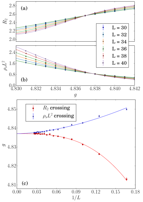
Figure 2: (Color online) (a) Binder ratio, $R_{2}$, and (b) scaled spin stiffness, $\rho_{s}L^{2}$, as functions of the coupling ratio $g$ for system sizes $L=30$, 32, $\dots$, 40. Crossings of the curves for pairs of system sizes $L$ and $L+2$ define finite-size estimates $g_{c}^{R}(L)$ and $g_{c}^{\rho}(L)$ of the critical point, which are are fitted to the form of Eq. (16) in panel (c). Enforcing a common value of $g_{c}$ in both fits gives the $L\to\infty$ critical point as $g_{c}=4.83704(6)$ and the irrelevant exponent as $\omega=-0.31(5)$ for $R_{2}$ and $\omega=0.82(5)$ for $\rho_{s}L^{2}$.

Figure 2(a) shows $R_{2}$ as a function of $g$ in the neighborhood of the critical coupling ratio for various system sizes. We have performed simulations for all even-length sizes $L=6$, 8, 10, …, 40, but here we present only the $L=30$, 32, …, 40 data for clarity. Analogous curves for the scaled spin stiffness, $\rho_{s}L^{2}$, are shown in Fig. 2(b), again only for system sizes $L=30$, 32, …, 40. In both cases, the system sizes are sufficiently large that the crossing points exhibit only a very weak dependence on $L$ on the scale used in the figure, and both sets of data may be used independently to show that the QCP is located at $g_{c}\simeq 4.837(1)$. A detailed analysis is required to obtain the most precise results attainable, free of any finite-size effects, and we first discuss the general scaling behavior of $g_{c}$ before presenting our numerical results.

III.1 Scaling Forms for Critical-Point Estimators

To describe the evolution of the crossing points with $L$, we perform a systematic extrapolation of the finite-size data to the thermodynamic limit by extracting the crossing points between data sets for all pairs of system sizes, $L$ and $L+2$, based on polynomial interpolations. Figure 2(c) shows the crossing points $g_{c}^{R}(L)$ and $g_{c}^{\rho}(L)$ obtained in this manner.

For any quantity probing a singularity in the thermodynamic limit, one may define a size-dependent critical point $g^{\prime}_{c}(L)$. In general, this quantity is expected to shift by an amount proportional to $L^{-1/\nu}$ with respect to the true infinite-size critical point, $g_{c}(\infty)$ (hereafter denoted for simplicity by $g_{c}$), i.e. for large $L$,

$$g_{c}(L)=g_{c}+aL^{-1/\nu},$$ (15)

where $\nu$ is the standard correlation-length exponent. However, with a definition based on crossing points of a dimensionless quantity computed for two different sizes, the leading corrections cancel and the convergence is faster,

$$g_{c}(L)=g_{c}+aL^{-(1/\nu+\omega)},$$ (16)

where $\omega>0$ is the dominant irrelevant exponent. In practice, with data fits to a rather limited range of available system sizes, the corrections to Eq. (15) contained in Eq. (16) will have exponents and prefactors that deviate from their asymptotic values due to the neglected corrections of higher order in $1/L$ and therefore these should be considered as “effective” quantities.

The above forms are applicable in the absence of logarithmic corrections, but such corrections are the primary focus of our study and are expected at $D=D_{c}$. Kenna has derived the modified form of Eq. (15) for classical systems with logarithmic corrections rkbc ; rkb ,

$$g_{c}(L)=g_{c}+aL^{-1/\nu}\ln^{\hat{\lambda}}L,$$ (17)

where the exponent of the logarithm for the 4D O$(3)$ universality class is $\hat{\lambda}=-1/22$. For the crossing points, Eq. (16) is modified to

$$g_{c}(L)=g_{c}+aL^{-(1/\nu+\omega)}\ln^{\hat{c}}L,$$ (18)

as shown in Appendix A, where $\hat{c}=\hat{\lambda}$ if the subleading term $L^{-\omega}$ has no multiplicative logarithmic correction, but is altered by an unknown amount if it does. Under the circumstances, with a number of unknowns and with simulation data only for a restricted range of system sizes, we fit our data using not Eq. (18) but instead the purely algebraic form of Eq. (16) with $\nu=1/2$ and $\omega$, the effective value of the subleading exponent over the fitting range, treated as a different fitting parameter for the separate quantities $R_{2}$ and $\rho_{s}L^{2}$.

III.2 Numerical Determination of $g_{c}$

We take both pairs of fitting parameters $a$ and $\omega$ in Eq. (16) to be independently free for the two datasets $g_{c}^{R}(L)$ and $g_{c}^{\rho}(L)$, but impose the constraint that the curves have the same $g_{c}$. As shown in Figs. 2(a) and 2(b), we obtain good fits to both functions, meaning with a reduced $\chi^{2}$ (per degree of freedom, hereafter denoted $\chi_{r}^{2}$) close to $1$, to the data for all system sizes ($L\geq 6$). These allow us to conclude that $g_{c}=4.83704(6)$, where the numbers in parenthesis denote the expected errors (one standard deviation) in the preceding digit, i.e. the relative error on $g_{c}$ is approximately one part in $10^{5}$. If we allow independent parameters $g_{c}^{R}$ and $g_{c}^{\rho}$ in the fits to the two data sets, both estimates of the critical point are statistically consistent with this $g_{c}$, albeit with somewhat larger error bars.

We note here that the values we find for the subleading exponent, $\omega=-0.31(5)$ for the $R_{2}$ data and $\omega=0.82(5)$ for the $\rho_{s}L^{2}$ data, lie far from a common asymptotic value. Thus indeed $\omega$ should be considered as an effective exponent accounting for crossover effects in system size, neglected higher-order irrelevant fields, and the expected weak logarithmic corrections. However, the good match obtained between the two extrapolated $g_{c}$-estimators, especially when approaching the infinite-size value from different directions, would not be expected in the presence of any corrections not taken sufficiently into account by the fitting functions. Thus we believe the error bar on $g_{c}$ quoted above to be completely representative of all statistical and systematic uncertainties, in the sense that any remaining systematic errors due to the fitting form should be smaller than the statistical errors. The tests we perform on the critical scaling behavior around the QCP in the subsequent sections also support this statement.

IV Size-Dependent Logarithmic Corrections at the QCP

The critical O($N$) $\phi^{4}$ theory, by which is meant the theory at the upper critical dimension and at the critical point, obeys many fundamental and universal properties, some of which depend on $N$ while others are $N$-independent. In Ref. Kenna2004 it was shown that the zeros of the partition function (Lee-Yang zeros) YangLee1952 , and hence the thermodynamic functions, obey a finite-size scaling theory, which was derived by renormalization-group methods. These perturbative arguments demonstrate that there are multiplicative logarithmic corrections in the system-size dependence of derivable thermodynamic functions, which are closely linked to those of the Lee-Yang zeros and, furthermore, are independent of $N$ for odd $N$. This leads to the key practical observation that size-dependent logarithmic corrections in physical observables such as the magnetic susceptibility and the specific heat at the critical point follow a universal, $N$-independent form when $N=3$. Here we provide a non-perturbative calculation of the magnetic susceptibility, $\chi(\mathbf{Q}_{\rm AF},L)$ [Eq. (8)], for systems of finite $L$ at the QCP, $g_{c}$, of the $(3+1)$-dimensional O($3$) transition to test the predicted logarithmic corrections.

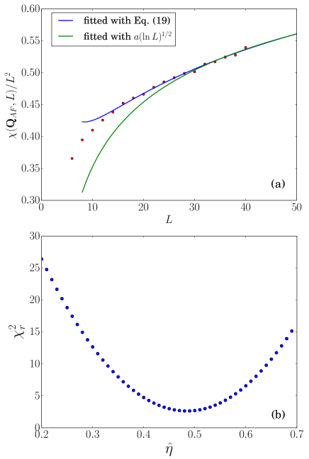
Figure 3: (Color online) (a) QMC data for $\chi(\mathbf{Q}_{\rm AF},L)/L^{2}$ obtained at $g=4.837$ for all even system sizes from $L=6$ to $40$. Solid lines are fits to $a(\ln L)^{1/2}$ (green) and to Eq. (19) (blue). We apply the square-root fit only for system sizes $L\geq 30$ and the optimal value of the fitting parameter is $a=0.274$. The two-parameter fit is made to the data for all system sizes $L\geq 14$ and yields optimal parameters $a=0.522$, $b=-1.317$. (b) Reduced $\chi^{2}$ values obtained by fitting $\chi(\mathbf{Q}_{\rm AF},L)/L^{2}$, for $14\leq L\leq 40$, to the form (19), but with the exponent $1/2$ replaced by a parameter $\hat{\eta}$. The optimal $\chi_{r}^{2}$ value is obtained at $\hat{\eta}\simeq 0.5$, consistent with the prediction of Ref. Kenna2004 .

The universal form of the magnetic susceptibility at the critical point in a finite-size system is given by Kenna2004

$$\chi(\mathbf{Q}_{\rm AF},L)=aL^{2}[\ln L]^{1/2}\left[1+b\frac{\ln(\ln L)}{\ln L}\right]\!\!,$$ (19)

with non-universal but $L$-independent parameters $a$ and $b$. We used this expression with a fixed value $g=4.837$, which is within the standard deviation of the $g_{c}$ value found in Sec. III, to investigate the logarithmic corrections to the $L$-dependence of $\chi(\mathbf{Q}_{\rm AF},L)$. We calculate the susceptibility at the ordering wave vector, $\mathbf{Q}_{\rm AF}=(\pi,\pi,\pi,\pi)$, for systems of all even sizes from $L=6$ to 40. As in Sec. III, the scaling predictions under test are valid for a 4D theory and again we use the critical contour $T^{-1}=kL$ with $k=1$.

Figure 3(a) shows our results for the critical magnetic susceptibility normalized by $L^{2}$. In the absence of logarithmic corrections, $\chi(\mathbf{Q}_{\rm AF},L)/L^{2}$ would be constant and the curve would be a flat line. Instead we observe that a reasonable account of the data for our larger system sizes ($L\geq 30$) requires a fit of the form $\chi(\mathbf{Q}_{\rm AF},L)/L^{2}=a(\ln L)^{1/2}$, as anticipated in Ref. Kenna2004 . However, for a more quantitative fit over the full size range available, we find [Fig. 3(a)] that it is necessary to include the predicted subleading logarithmic correction in Eq. (19).

To examine the sensitivity of these results to the exponent $1/2$ of the multiplicative logarithm in Eq. (19), we replace this predicted exponent by a variable ${\hat{\eta}}$. We determine this exponent by calculating the goodness of fit $\chi_{r}^{2}$ as a function of $\hat{\eta}$. As Fig. 3(b) makes clear, the best fits are indeed obtained close to $\hat{\eta}=0.5$, in complete consistency with Eq. (19).

From the fact that our exact numerical data confirm not only the leading but also the subleading corrections to scaling, we conclude that obvious logarithmic corrections can be observed in the size-dependence of the thermodynamic functions at the QCP. This result also demonstrates that our determination of $g_{c}$ is sufficiently precise to study logarithmic corrections without significant distortions arising from uncertainties in its value.

V Sublattice Magnetization

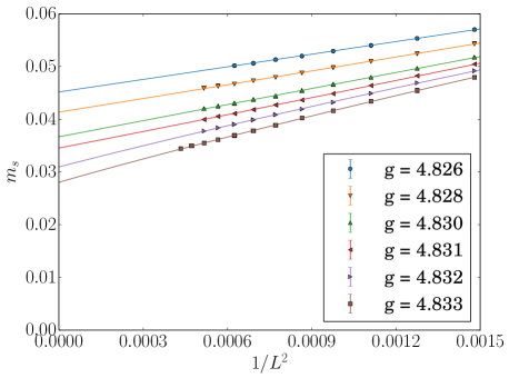
Figure 4: (Color online) Staggered magnetization, defined for each system size as $m_{s}(L)=[3\langle m_{2z}^{2}(L)\rangle]^{1/2}$, shown as a function of $1/L^{2}$ for a range of coupling ratios $g$ near $g_{c}$. Polynomial fits of cubic order were used to extrapolate $m_{s}(L)$ to the thermodynamic limit; the temperature in all cases was $T=1/L$. Error bars on all points are smaller than the symbol sizes.

Physical condensed-matter systems at continuous QPTs are generally in the thermodynamic limit, and size-scaling measurements of the type easily performed in QMC simulations (Sec. IV) are not a realistic experimental option. However, as discussed in Sec. I, multiplicative logarithmic corrections are expected in a range of physical quantities close to the QCP. The primary physical observables in the quantum antiferromagnet are the zero-temperature staggered magnetization, $m_{s}(g_{c}-g)$, and the Néel temperature, $T_{N}(g_{c}-g)$. Calculating these quantities in the thermodynamic limit is significantly more challenging than studies of size-dependence, as careful extrapolations of finite-size data are required. Here and in Sec. VI we describe and then implement appropriate measures for extrapolating to infinite system size and, for $m_{s}$, to zero temperature, thereby revealing the logarithmic corrections to both $m_{s}$ and $T_{N}$.

We compute the staggered magnetization according to Eq. (7) for coupling ratios as close to $g_{c}\simeq 4.837$ as $g=4.834$. For a given value of $g$, we calculate the squared quantity $\langle m^{2}_{sz}(g,L)\rangle$ over a range of system sizes. As shown in Fig. 4, the staggered magnetization clearly decreases with increasing $L$ and converges towards a fixed limit, suggesting a controlled extrapolation even very close to the QCP. Definitive extrapolation to the thermodynamic limit in this regime is a complex issue, and a discussion of several technical points is in order before analyzing our results.

V.1 Extrapolation scheme

First, most of the simulations in this section are performed at a temperature $T=1/L$, such that the extrapolation $L\rightarrow\infty$ includes both system size and temperature. Because the system is ordered for sufficiently low $T$ and the order parameter converges quickly to a non-zero value below the ordering temperature, one may use the form $T=aL^{-b}$ with arbitrary prefactor $a>0$ and exponent $b>0$ to study the $T\to 0$ magnetization as a function of $L$. These conditions for obtaining a ($T\to 0,L\to\infty$) extrapolation of the order parameter for $g<g_{c}$ contrast with the need to follow the contour $T=aL^{-1}$ ($a=1/k$; $b=1$ when $z=1$) in Secs. III and IV for studies of the QCP. Although large values of $a$ and $b$ should improve the convergence, in practice one must consider the balance between computation time and convergence rate, and the choice $a=1$, $b=1$ works well in most cases. However, for coupling ratios very close to the QCP, the temperature may be a significant fraction of $T_{N}$ and thus $m_{s}(g,L)$ could be far from its zero-temperature value. We have therefore performed additional simulations at $T=1/(2L)$ to verify that the extrapolation does remain well controlled and fully representative of the thermodynamic limit in temperature as well as in system size.

Second, in contrast to Sec. III, where we used the non-trivial power-law scaling forms (16) known to be appropriate for extrapolating the location of a critical point, the ground-state order parameter inside the Néel phase can be extrapolated by using simple polynomial fits. To obtain $m_{s}$, one may extrapolate the squared quantity and then take its root afterwards or take the square root for each system size before extrapolating (the procedure followed in Fig. 4); the corresponding polynomials are

$$m^{2}_{sz}(g,L) = a(g)+b(g)L^{-2}+c(g)L^{-3}+\dots,$$ (20)

$$\sqrt{m^{2}_{sz}(g,L)} = a^{\prime}(g)+b^{\prime}(g)L^{-2}+c^{\prime}(g)L^{-3}+\dots$$ (21)

Here the leading $L$-dependence in the extrapolation of a non-vanishing order parameter, at fixed $g$ inside the ordered phase, is known cardy to be $L^{2-d-z}$ due to the dimension-dependent power-law decay of the transverse correlation function. Here $d+z=d+1=D=D_{c}=4$, and the resulting leading $1/L^{2}$ dependence is shown clearly in Fig. 4. Because these procedures use a polynomial of finite order to approximate physical behavior containing, in principle, an infinite number of corrections, the extrapolated value of $m_{s}$ obtained with the forms (20) and (21) will not be exactly the same, but for reliable fits they should agree within statistical errors.

We stress that no logarithmic corrections are expected in this case, meaning that on grounds of principle they should not be present in the asymptotic large-$L$ corrections to a non-zero-valued order parameter. This non-critical behavior contrasts with the case of the shift in the critical point discussed in Sec. III, where logarithmic corrections should in principle be present, although we concluded that their effects are not detectable in practice.

Finally, however, non-trivial corrections may still be expected in the $L$ dependence of $\langle m^{2}_{sz}(g,L)\rangle$ for $g$ close to the QCP, where the order parameter is small, in the form of crossover behavior from near-critical at small system sizes to asymptotic ordered-state scaling at large $L$. Quite generally, no analytic functional forms are available for describing such crossovers, and great care is required to ensure that the asymptotic region, where Eqs. (20) and (21) are valid, has been reached. As $g\rightarrow g_{c}$, successively larger systems are required for this, and here we find that reliable extrapolations are no longer possible beyond $g=4.834$ because of the limits on system size set by the available computer resources.

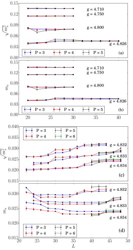
Figure 5: (Color online) Extrapolated values of the sublattice magnetization as a function of the largest system size included in the fit, for values $g$ near the QCP ($g_{c}\simeq 4.837$). Panels (a) and (b) include values of $g$ for which the extrapolations are stable for relatively small $L$; panels (c) and (d) show $g$ values very close to $g_{c}$, where the extrapolations require large sizes to stabilize. Results for different orders $P$ of the fitting polynomial are compared. The smallest system size included was determined using the $\chi_{r}^{2}$ criterion of Eq. (22). Panels (a,c) and (b,d) show respectively the results of extrapolations of $\langle m^{2}_{sz}(g,L)\rangle$ and $\langle m^{2}_{sz}(g,L)\rangle^{1/2}$, with the square root taken after the extrapolation in the former case.

In fits to the forms (20) and (21), it is necessary to select the order $P$ of the polynomial and the range of system sizes to include. The size of the error bars on the QMC data points has a significant influence here, because deviations from the leading $L^{-2}$ correction are easier to detect with smaller error bars. We have performed a systematic study using fits of orders $P=3$ to 6, including different system-size ranges. We characterize the quality of the fits using the standard reduced $\chi^{2}$ measure, and for a “good” fit we require that the optimal value must fall within three standard deviations of its mean, i.e. we demand that

$$\chi_{r}^{2}-1=\frac{\chi^{2}}{n_{L}-n_{p}}-1\leq 3\sqrt{\frac{2}{n_{L}-n_{p}}},$$ (22)

where $n_{L}$ is the number of data points (system sizes) and $n_{p}=P+1$ is the number of fitting parameters. For a given $P$ and largest system size $L$, we use all available system sizes down to a smallest size $L_{\rm min}$ for which the above condition is still satisfied. We then study the behavior as a function of $L$ for different $P$, and compare the values of $m_{s}$ obtained from extrapolations based on Eqs. (20) and (21). To estimate the error bars on the extrapolated $m_{s}(g)$, we performed additional polynomial fits with Gaussian noise (whose standard deviation is equal to the corresponding QMC error bars) added to the finite-size data. The standard deviation of the distribution of extrapolated $m_{s}(g)$ values defines the statistical error.

Figure 5 shows results for several values of $g$ approaching the QCP, with cases where the fits are relatively straightforward (further from $g_{c}$) shown in panels (a) and (b) and more challenging cases (closer to $g_{c}$) shown in panels (c) and (d). The upper panel in each group corresponds to the square root being taken after the extrapolation [Eq. (20)], while the lower corresponds to fitting the square root for each system size [Eq. (21)]. In panels (a) and (b), the extrapolated values are observed to be very stable with respect to the range of system sizes and the order of the polynomial, whereas panels (c) and (d) manifest some of the crossover behavior expected close to $g_{c}$, showing considerable variation as the maximum system size is increased. There are also significant differences between the two fitting procedures, until the largest system sizes where the extrapolations stabilize; we take the fact that the two types of fits give consistent results for these largest systems at all values of $g$ as an indication that the extrapolations are reliable. We have not been able to achieve good convergence based on system sizes up to $L=48$ for $g$ values closer to $g_{c}$ than those shown in Figs. 5(c) and (d). In these most challenging cases, our results show that it is better to use the fitting form of Eq. (21), extrapolating the square root of the staggered magnetization for each system. Regarding the quality of the fits obtained by varying the polynomial order, $P$, in Fig. 5, we find that extra terms in the fit scarcely justify the additional degrees of freedom lost in the determination of $\chi_{r}^{2}$. All of the results presented below were obtained by extrapolating $\sqrt{m_{s}^{2}}$ with polynomials of order $P=4$.

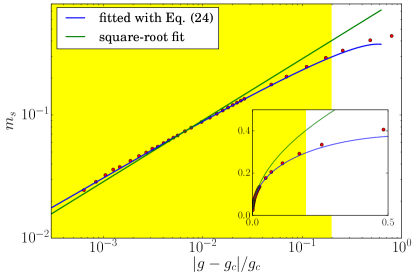
Figure 6: (Color online) Extrapolated staggered magnetization, $m_{s}$ at $T=0$, as a function of the distance from the QCP, using the value $g_{c}=4.83704$ determined in Sec. III. Error bars on the calculated data points are similar to or smaller than the symbol size. The closest point to $g_{c}$ is $g=4.834$. Lines show both the best fit by a pure square-root function [Eq. (23), green] and including the logarithmic correction factor predicted in Ref. Kenna2004 [Eq. (24), blue]. The fitting parameters of the logarithmic correction curve are $a=0.266(2)$ and $b=4.8(3)$. The yellow shading represents the approximate extent of the QC regime and is determined by including all data points described adequately (within a deviation of approximately $4\%$, see text) by the functional form of the logarithmic correction curve. The inset shows $m_{s}(g)$ and the QC regime on linear axes.

V.2 Thermodynamic Limit

With all of the above considerations, we are able to obtain reliable and high-precision extrapolations of the staggered magnetization in the thermodynamic limit for values of $g$ as close to the QCP as $|g-g_{c}|\simeq 0.003$. In Fig. 6 we show all of our data for $m_{s}(|g-g_{c}|)$ on logarithmic axes. If these data satisfied mean-field scaling alone, with no discernible logarithmic corrections, one would expect a curve of the form

$$m_{s}(g)=a|g-g_{c}|^{1/2},$$ (23)

but this (green line in Fig. 6) is manifestly unable to describe the data. For the zero-temperature order parameter, perturbative renormalization-group considerations applied to the O($N$) $\phi^{4}$ field theory at the upper critical dimension predict the form

$$m_{s}(g)=a|g-g_{c}|^{\beta}|\ln(|g-g_{c}|/b)|^{\hat{\beta}},$$ (24)

where $\beta=1/2$ is the mean-field exponent and the exponent of the multiplicative logarithmic correction is given by $\hat{\beta}=3/(N+8)$ Kenna2004 . A fit to this form, using $\hat{\beta}=3/11$ for $N=3$ (blue curve in Fig. 6), yields excellent agreement with the data all the way to our smallest values of $|g-g_{c}|$; the fitting parameters are $a=0.266\pm 0.002$ and $b=4.8\pm 0.3$. We note that the fit is very insensitive to the precise value of $b$, and for further analysis we fix this to $b=g_{c}$.

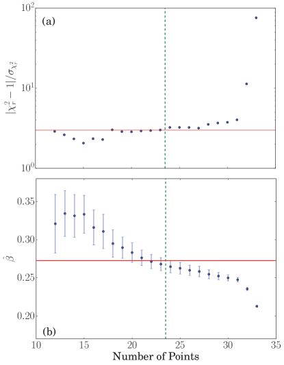
Figure 7: (Color online) Statistical analysis of the exponent of the logarithmic correction in Eq. (24). (a) Reduced $\chi^{2}$ value of the fit, normalized to the standard deviation, and (b) optimal value of the exponent shown as functions of the number of data points ($g$-values) used, beginning from the point closest to $g_{c}$ in Fig. 6. The vertical dashed line indicates the number of points, $N_{g}=23$, for which a $3\sigma$ criterion for $\chi_{r}^{2}$ [cf. Eq. (22)] is satisfied, as indicated by the horizontal line in panel (a). In panel (b), the error bars were computed by repeating the fits multiple times with Gaussian noise added to the $m_{s}$ data points. The horizontal line marks the predicted value $\hat{\beta}=3/11$.

To test the predicted exponent $\hat{\beta}=3/11$ in Eq. (24), we treat it as a free parameter and fit our data using different numbers of $g$ values, including all points closest to $g_{c}$ and studying the behavior as points further away from $g_{c}$ are added one by one. Figure 7 shows $\chi_{r}^{2}$ and $\hat{\beta}$ as functions of the number of data points fitted. With the exception of cases including the two points furthest away from $g_{c}$, all the fits appear reasonable, with $\chi_{r}^{2}<2$. However, by the properties of the $\chi^{2}$ distribution, a fit should be considered statistically acceptable only if a criterion analogous to Eq. (22) is satisfied, i.e. the largest number of data points for which $\chi_{r}^{2}-1$ remains less than three times its standard deviation ($3\sigma$) marks the boundary between good and poor fits. At this point we obtain $\hat{\beta}=0.268\pm 0.008$, which lies well within one standard deviation of the predicted value $3/11\approx 0.2727$. If more points are excluded, the fitted exponent evolves slowly [Fig. 7(b)] while remaining statistically well compatible with the predicted value. Because the fitting error increases, less weight should be placed on results including less data, and taking an error-weighted average over all the points below the cut-off line, $N_{g}=23$, in Fig. 7 yields $\hat{\beta}=0.279\pm 0.011$. We take this as complete confirmation of the predicted value.

As important as finding clear logarithmic corrections to scaling is that we have demonstrated their presence over a significant region around the QCP; indeed, most of the points we have computed are well described by Eq. (24). Including the multiplicative logarithmic correction converts an inadequate description of the data into an excellent one (Fig. 6) as far inside the Néel phase as $|g-g_{c}|/g_{c}\approx 0.2$, where the order parameter is already at $60\%$ of its maximum possible value ($m_{s}=1/2$, at which point no quantum fluctuation effects remain). This improvement is clearer still in the inset of Fig. 6, which shows the results on linear axes. Under the assumption that data points at large $|g-g_{c}|$ no longer fall on the fitted curve because they lie outside the region controlled by the QCP, we can determine the size of the critical region based on a threshold maximum deviation of the data from the curve. Although the choice of threshold value is somewhat arbitrary, the $|g-g_{c}|/g_{c}\leq 0.2$ region indicated by the yellow shading in Fig. 4 reflects a threshold of approximately $4\%$, which lies well above achievable experimental uncertainties. We comment in Sec. VII on the utility of our results for the case of TlCuCl₃.

VI Néel temperature

We turn next to the scaling form of the Néel temperature, $T_{N}(g)$, near the QCP. Unlike the $T=0$ order parameter, as far as we are aware there is no prediction from perturbative field-theoretical calculations including logarithmic corrections for the scaling form of finite-$T$ critical points at the upper critical dimension. Close to a QCP, the general power-law form without logarithmic corrections is discussed in Ref. rs , but one may also expect a multiplicative logarithmic term as in the other quantities we have discussed. We first derive the exponent of the logarithm for the O($3$) transition in 3+1 dimensions, based on the known scaling properties of related quantities. We then present our QMC calculations of $T_{N}$ for the Heisenberg model on the double cubic lattice and test our prediction.

VI.1 Scaling hypothesis

In a path-integral construction in imaginary time, the size of the system in the time dimension is proportional to the inverse temperature, $\beta=1/T$. This can be considered as a length, $L_{\tau}$, on a parallel with the spatial lengths, $L$, of a $d+1$-dimensional system. If the spatial lengths are taken to infinity in all directions, what remains is a single finite length, $L_{\tau}$, for the effective system, and finite-size scaling in this length corresponds to finite-$T$ scaling in the original quantum system Chakravarty88 .

Without logarithmic corrections, by analogy with the finite-$L$ shift of the critical point discussed in Sec. III.1, the same type of shift as in Eq. (15) can be expected because $z=1$. Thus

$$g_{c}(T)-g_{c}(0)\sim L_{\tau}^{-1/\nu},$$ (25)

as a consequence of the finite temporal size, and the scaling behavior is $T_{N}\sim(g_{c}-g)^{\nu}$, as discussed in detail in Ref. rs . In the case of spatial finite-size scaling, with all lengths finite, the shifted critical point (sometimes called the pseudo-critical point) is not a singular point, but the singularity develops as $L\to\infty$. By contrast, in the finite-$T$ case in $d=3$ spatial dimensions, the shifted point is a true (classical) phase transition, although from a scaling perspective this difference is not relevant.

In order to discuss logarithmic corrections, it is useful to first express $T_{N}$ using a macroscopic, zero-temperature energy scale of the system that vanishes as $g\to g_{c}$ rs . For the spin system considered here, the only such energy scale is the spin stiffness, $\rho_{s}$. According to Ref. Fisher1989 , the scaling form of this quantity in the ordered phase when $z=1$ is

$$\rho_{s}\sim(g_{c}-g)^{\nu(d-1)}.$$ (26)

Consistency with the result $T_{N}\sim(g_{c}-g)^{\nu}$ then gives the scaling of the critical temperature for $d=3$,

$$T_{N}^{2}\sim\rho_{s},$$ (27)

where the mismatch in units is compensated by a power of the non-singular spin-wave velocity rs (Sec. VIC), which can be neglected here. Our basic hypothesis is that this proportionality, which is the singular part of a relationship based on matching scaling dimensions, applies in all respects at the upper spatial critical dimension ($d=3$ for $z=1$), such that logarithmic corrections to $T_{N}$ arise solely due to the logarithmic corrections intrinsic to $\rho_{s}$.

Fisher et al. Fisher1989 have shown that the critical spin stiffness can be expressed as $\rho_{s}\sim\xi^{2}f$, where $\xi$ is the correlation length and $f$ is the free-energy density. The logarithmic corrections to both $\xi$ and $f$, presented by Kenna in Ref. rkbc , are

$$\xi\sim|g-g_{c}|^{-\nu}\ln^{\hat{\nu}}(|g-g_{c}|),$$ (28)

with $\hat{\nu}=5/22$ for the relevant universality class, and

$$f\sim|g-g_{c}|^{4\nu}\ln^{\hat{\alpha}}(|g-g_{c}|),$$ (29)

with $\hat{\alpha}=1/11$. The logarithmic correction to $\rho_{s}$ is therefore given by

$$\rho_{s}\sim|g-g_{c}|^{2\hat{\nu}}\ln^{2\hat{\nu}+\hat{\alpha}}(|g-g_{c}|),$$ (30)

and by combining these results with Eq. (27) we obtain

$$T_{N}\sim|g-g_{c}|^{\nu}\ln^{\hat{\tau}}(|g-g_{c}|),$$ (31)

where $\hat{\tau}=\hat{\nu}+{\hat{\alpha}}/{2}$. From the values of $\hat{\nu}$ and $\hat{\alpha}$ given above rkbc , we obtain the prediction $\hat{\tau}=3/11$, which is remarkable in that the exponent in the logarithmic correction to $T_{N}$ should be the same as the one in the sublattice magnetization, $\hat{\tau}=\hat{\beta}$ (24).

Because the zero-temperature order parameter is a consequence purely of quantum fluctuations, whereas the classical ordering temperature is a consequence primarily of thermal fluctuations, there is a priori no reason to expect that the two should have the same form. Exact numerical calculations are therefore uniquely positioned to provide qualitatively new information in this case. We note that this equality applies to the phase transitions of O($N$) models for all values of $N$; because $\hat{\nu}=(N+2)/[2(N+8)]$ and $\hat{\alpha}=(4-N)/(N+8)$ rkbc , we obtain $\hat{\tau}=3/(N+8)$, the same value as the exponent $\hat{\beta}$ in Eq. (24). Thus we predict that, in the neighborhood of $g_{c}$, $T_{N}(g)$ will be proportional to $m_{s}(g,T=0)$, with no multiplicative logarithmic factors, for all values of $N$; this result was reported for the $N=3$ case in a previous QMC study Jin2012 , which we now extend sufficiently close to the QCP to observe the cancellation of logarithmic terms.

VI.2 QMC calculations

Calculating $T_{N}(g)$ within our QMC simulations is similar to obtaining $g_{c}$ in Sec. III, but with some important differences of detail. The calculations of Sec. III were performed for a genuinely 4D system, with the imaginary-time axis treated on the same footing as the spatial dimensions. At finite temperatures, this symmetry is broken and the system is 3D with a separate temperature variable, which determines the finite thickness of the time dimension even when $L\to\infty$. Both the Binder ratio [Eq. (9)] and the spin stiffness [Eq. (11)] are size-independent quantities at the thermal phase transition and hence remain valuable indicators, although the appropriately scaled spin stiffness for the 3D transition is now $\rho_{s}L$ (instead of $\rho_{s}L^{2}$, used for analyzing the 4D $T=0$ transition in Sec. III) Jin2012 .

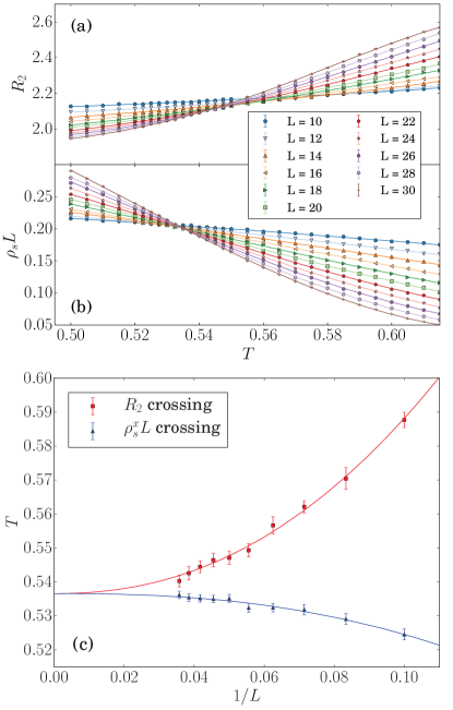
Figure 8: (Color online) Procedures used to extract the Néel temperature, $T_{N}(g)$, illustrated for the case $g=4.71$. (a) Binder ratio $R_{2}$ as a function of $T$ for system sizes $L=10$, 12, …, 30. (b) Scaled spin stiffness $\rho_{s}L$ as a function of $T$ for the same values of $L$. Error bars are smaller than the symbol sizes. Crossings of these lines are extracted using polynomial fits and the results are used to obtain finite-size estimates for quantities $T_{N}^{R}(L)$ and $T_{N}^{\rho}(L)$. (c) Fits to data for systems of all sizes ($L\geq 6$) of the two size-dependent crossing estimators using functions of the form $T_{N}(L)=T_{N}(\infty)+a/L^{1/\nu+\omega}$. Enforcing the same constant $T_{N}(\infty)\equiv T_{N}$ for the $R_{2}$ and $\rho_{s}L$ crossings gives $T_{N}=0.5363(13)$ with irrelevant exponents $\omega\approx 0.8(2)$ for $R_{2}$ and 1.1(3) for $\rho_{s}L$ ($1/\nu\approx 1.42$ for the relevant 3D universality class).

For each value of the coupling ratio $g$ within the Néel phase ($g<g_{c}$), we compute $R_{2}$ and $\rho_{s}L$ for a range of system sizes and perform finite-size-scaling extrapolations to deduce the Néel temperature, $T_{N}(g)$, in the thermodynamic limit. Similar to Sec. III, we first obtain the crossings of the $R_{2}(T)$ and $\rho_{s}L(T)$ data for different system sizes using polynomial fits, as shown in Figs. 8(a) and 8(b) for $g=4.71$. The crossing points of both quantities for each successive pair of system sizes, $T_{N}(g,L)$ and $T_{N}(g,L+2)$, are used to extrapolate towards the value $T_{N}(g,L\to\infty)$ from above and below, using power-law forms analogous to Eq. (16). We note that, as in the analysis leading to $g_{c}$ (Sec. III.2), the data points obtained for $R_{2}(L,T)$ and $\rho_{s}L(L,T)$ using systems of all sizes ($L\geq 10$) fall within a $3\sigma$ criterion analogous to Eq. (22) for this type of fit. The extrapolation of $T_{N}(g,L\to\infty)\equiv T_{N}(g)=0.5363(13)$ for $g=4.71$ is shown in Fig. 8(c).

We comment here that our determination of $T_{N}(g)$ for $g$ close to $g_{c}$ is rather less precise than our determination of $m_{s}(g)$. The fundamental difference in character of the two quantities, and hence of their calculation, causes the estimators for $T_{N}(g)$ [the approximate crossings in Figs. 8(a) and 8(b)] to have larger error bars and finite-size effects. Further, the error bars of the crossing points grow rapidly as $g\to g_{c}$, while the decrease in $T_{N}$ leads to longer simulation times (because the space-time volume is proportional to $L^{3}/T$). After detailed error control, the closest reliable data point to the QCP is $g=4.831$, for which $|g-g_{c}|$ is twice as large as for the closest $m_{s}(g)$ point (Sec. V). We have nevertheless obtained 19 reliable data points, within the QC regime determined from $m_{s}(g)$ (Fig. 6) and down to unprecedentedly low temperatures, which are fully sufficient to test for evidence of logarithmic corrections to $T_{N}(g)$.

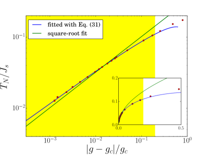
Figure 9: (Color online) Normalized Néel temperature, $T_{N}/J_{s}$, as a function of the distance from criticality, $|g-g_{c}|$. The closest point to $g_{c}\approx 4.837$ is $g=4.831$. Lines show both the best fit by a pure square-root function (green) and using a logarithmic correction factor with exponent $\hat{\tau}=3/11$ [Eq. (31), blue]. The yellow shading represents the QC regime and is determined from Fig. 5. The inset shows $T_{N}(g)$ on linear axes.

The Néel temperature has units of energy and clearly depends on the overall energy scale of the system. Ideally, it should be normalized by an intrinsic energy scale of the system to give a dimensionless quantity. In Ref. Jin2012 it was shown that $T_{N}(|g-g_{c}|)$ normalized to the microscopic energy scale $J_{s}$, given by the sum of all couplings of a spin to its neighbors, yields a remarkably system-independent result for Heisenberg antiferromagnets with three different dimerization patterns; for the double cubic lattice, $J_{s}=J(6+g)$. Other authors Oitmaa2012 ; Kao2013 have suggested that the appropriate normalization is given by a macroscopic quantity, the spatially averaged spin-wave velocity, $\sqrt{c_{x}c_{y}c_{z}}$ (which, it should be noted, does not have units of energy and requires an unknown dimensionful constant). We begin by taking the former approach and return below to address the latter.

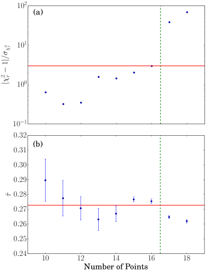
Figure 10: (Color online) Statistical analysis of the exponent of the logarithmic correction in Eq. (31), performed by replacing the predicted value $3/11$ with a fitting parameter $\hat{\tau}$. (a) Reduced $\chi^{2}$ value of the fit, normalized to the standard deviation, and (b) optimal value of the exponent, both shown as functions of the number of data points ($g$-values) used, beginning from the point closest to $g_{c}$ in Fig. 9. The vertical dashed line indicates the number of points, $N_{g}=16$, included in the fit below which $\chi_{r}^{2}$ satisfies a $3\sigma$ criterion analogous to Eq. (22), as indicated by the horizontal line in panel (a). In panel (b), the error bars were computed by repeating the fits multiple times with Gaussian noise added to the $T_{N}$ data points. The horizontal line marks the predicted value $\hat{\tau}=3/11$.

The relationship between $T_{N}/J_{s}$ and $|g-g_{c}|$ is presented in Fig. 9. Once again we show a mean-field scaling line for comparison and once again it cannot provide an adequate fit, suggesting that logarithmic corrections are indeed present. However, a fit to our predicted form, given by Eq. (31) with $\hat{\tau}=3/11$, describes the data very well, even at the limits of the region classified as QC based on the $m_{s}(g_{c}-g)$ fit in Fig. 5.

For a fully quantitative test of the exponent we predict for the multiplicative logarithmic term in Eq. (31), we substitute a free exponent $\hat{\tau}$ for the fixed value $3/11$ and optimize it using fits with different windows of $g$-values. This analysis is precisely analogous to that performed for $m_{s}$ in Fig. 7. The behavior of $\chi_{r}^{2}$ and of the optimized exponent, with error bars again estimated using the method of numerical Gaussian noise propagation, is presented in Fig. 10. By taking the inverse-variance-weighted average over all results for which $\chi_{r}^{2}$ is acceptable, we obtain $\hat{\tau}=0.275(2)$, in excellent agreement with the prediction $\hat{\tau}=3/11\simeq 0.2727$. We conclude that the multiplicative logarithmic correction to $T_{N}(g)$ is, to within our error bars and in agreement with a straightforward scaling argument based on the spin stiffness (Sec. VIA), identical to the $m_{s}(g)$ correction in Eq. (24).

VI.3 Spin-wave velocity

The spin-wave velocity, $c$, is uniform in the primary axial directions on the double cubic lattice. As discussed in Sec. II, it can be calculated most straightforwardly and most accurately in the SSE framework from the spatial and temporal winding-number fluctuations in Eq. (13) to define the space-time-isotropic criterion of Eq. (14), which contains the velocity Kaul2008 ; Jiang2011 ; Kao2013 ; Sen2015 . This technique remains well-defined throughout the critical regime and is expected not to be affected by logarithmic corrections; it was shown in Ref. Sen2015 , which we follow for technical details, that the winding-number approach produces the correct result for $c$ in the Heisenberg chain, a system known to have strong logarithmic corrections to scaling.

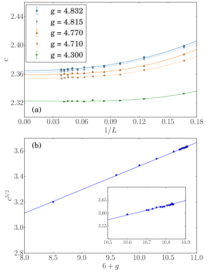
Figure 11: (Color online) Calculation of the spin-wave velocity. (a) Velocities $c(L)$ obtained for systems of sizes from $L=6$ to 26 at different values of the coupling $g$ and extrapolated using Eq. (32). (b) Extrapolated velocities $c(g)$ as a function of the microscopic energy scale $6+g$. Error bars are mostly hidden inside the symbols. The solid line is a linear fit and the inset magnifies the region close to $g_{c}$.

In Fig. 11(a) we show the results for $c(g,L)$ of calculations on finite systems of even sizes up to $L=26$, which we extrapolate to the thermodynamic limit using the relation

$$c(g,L)=c(g)+a(g)/L^{2}+b(g)/L^{3}.$$ (32)

This form is found empirically Sen2015 to provide a very good reproduction of the data and numerical errors due to finite-size effects in the critical regime are clearly small. Figure 11(b) shows the results for the extrapolated spin-wave velocities $c(g)$ of the infinite system, by comparing the macroscopic scale $c^{3/2}$ with the microscopic quantity $6+g$ discussed above. The almost perfect linearity demonstrates that the two effective energy scales are very closely related, which can be expected from the fact that the velocity of a spin excitation depends directly on the net interaction of a single spin, and both are perfectly valid choices for the normalization of $T_{N}$. A graph completely analogous to Fig. 9, showing a logarithmic correction with the same exponent $\hat{\tau}=3/11$, is obtained if $c^{3/2}$ is used to normalize $T_{N}(g)$.

VI.4 Relation between $T_{N}$ and $m_{s}$

In experiment it is often difficult to relate an external control parameter to the microscopic coupling constants of a model Hamiltonian. In a quantum antiferromagnet, some aspects of this problem can be circumvented by studying the relationship between $T_{N}$ and $m_{s}(T=0)$ directly, without reference to the control parameter, $g$. A universal relationship between these macroscopic and measurable quantites would be of considerable experimental utility in characterizing the nature of critical phenomena without recourse to detailed microscopic knowledge of the system parameters (such as the pressure dependence of the exchange couplings in TlCuCl₃). Although an experimental test Merchant2014 of the linear relationship between $T_{N}$ and $m_{s}$ Jin2012 indicated satisfactory agreement close to the QCP, the issue of how best to normalize $T_{N}$ was not addressed. We use our systematic data spanning the entire QC regime to test the limits of linear proportionality and discuss the normalization of $T_{N}$.

In Ref. Jin2012 , where a universal linear relation was found in three different models, the authors articulate a mean-field argument based on semiclassical considerations for a direct proportionality of $T_{N}$ to the effective spin order gauged by $m_{s}$ at $T=0$. In Ref. Oitmaa2012 , these arguments were elucidated in a field-theory context, where it was stated that logarithmic corrections should be negligible for linear proportionality to emerge. In fact these arguments can be reduced to the statement that it should be possible to treat quantum and thermal fluctuations independently, with no mutual interference of their effects Jin2012 . If one considers that mean-field exponents are valid in high-dimensional systems $(D>D_{c})$ because thermal fluctuations become independent of quantum fluctuations when the phase space is sufficiently large, then it appears that weak logarithmic corrections could enter the relationship of $T_{N}$ to $m_{s}$ at $D=D_{c}$. This possibility, also motivated by the (then) unknown form of the logarithmic corrections to $T_{N}$, was investigated directly by QMC simulations for the cubic lattice Kao2013 , but the results were not conclusive (claims concerning the observation of logarithmic corrections are not justified by the available data range). Here we have presented scaling arguments (Sec. VIA) and numerical data (Sec. VIB) demonstrating that the logarithmic corrections to $m_{s}$ and $T_{N}$ have precisely the same form, setting their linear relationship in this class of system on a far firmer foundation.

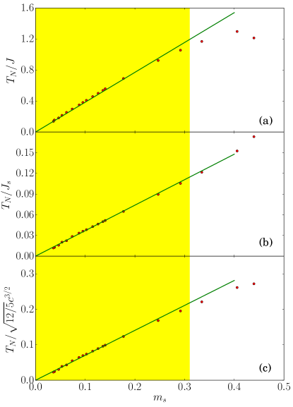
Figure 12: (Color online) Relationship between $T_{N}$ and $m_{s}$, using different normalizations of $T_{N}$; in (a) by the intra-cube coupling $J=1$, in (b) by the sum of couplings $J_{s}=6+g$, and in (c) by the spin-wave velocity in the form $\sqrt{12/5}c^{3/2}$. The lines are linear (proportionality) fits to the small-$m_{s}$ points and the yellow shaded areas denote the QC regime determined from $m_{s}(g)$ in Fig. 5.

Our data from Secs. V and VI can be used to probe the $T_{N}(m_{s})$ relation in detail and confirm that linearity extends much closer to the QCP than previous studies could show. Because our results are for a single type of dimerized model, we are not able to address the question of a universal prefactor Jin2012 . However, we are able to make a definite statement regarding logarithmic corrections in the relationship between $T_{N}$ and $m_{s}$. Figure 12 shows our data, taken from Figs. 6 and 9, in the form $T_{N}(m_{s})$, with the implicit control parameter $g$ effectively eliminated. In panel (a), $T_{N}$ is simply normalized by the energy scale, the interdimer coupling $J=1$; in panel (b), we have normalized $T_{N}$ by the composite scale $J_{s}=6+g$ (where $g$ can be considered a function of $m_{s}$), as in Fig. 9; in panel (c), we have normalized $T_{N}$ using the correctly scaled spin-wave velocity, $c^{3/2}$. The shaded regions again signify our definition of the critical region, based on the strict critical scaling of $m_{s}(g)$ in Fig. 5.

As shown in Ref. Jin2012 , we find in Fig. 12(b) that the linearity of $m_{s}$ and $T_{N}/J_{s}$ extends well beyond the QC regime; although our data were not selected to focus on this region, we do find complete agreement with previous calculations where the data overlap. Here we demonstrate that the essentially perfect linearity also extends much closer to $m_{s}=0=T_{N}$ ($g\to g_{c}$), and in particular that it remains valid throughout a regime with explicit logarithmic corrections in the individual quantities. Although we cannot show that the linear relationship extends all the way to the QCP, our data certainly suggest that this is the case, i.e. that it can also be considered a universal property of the QC regime. To the extent that linearity of $m_{s}$ and $T_{N}$ is a consequence of the decoupling of thermal and quantum fluctuations, this independence appears to extend from strongly ordered systems, where no logarithmic corrections are expected, to the most strongly fluctuating QC systems. The linear relationship we have demonstrated verifies in full our scaling prediction that the logarithmic corrections to $T_{N}(g)$ have the same exponent, $\hat{\tau}=\hat{\beta}=3/11$, as $m_{s}(g)$. We also note that the normalization of $T_{N}$ has no effect (beyond the prefactor) on the linear relationship in the QC regime, but that deviations from linearity clearly differ at higher $m_{s}$.

We close by considering in more detail the case where $T_{N}$ is normalized by $c^{3/2}$ [Fig. 12(c)], with a view to making quantitative comparisons with field-theory predictions Oitmaa2012 . The explicit relationship is

$$T_{N}=\gamma{c^{3/2}}\sqrt{\frac{{12}}{5}}m_{s},$$ (33)

where $\gamma=\langle\phi\rangle/m_{s}$ is the dimensionful prefactor relating the expectation value of the un-normalized field $\phi$ in the action to the order parameter $m_{s}$ of the lattice model. In the dimensionless units of our work ($J=1,\hbar=1$, …), we obtain $\gamma=0.6998\pm 0.0016$, thereby providing a bridge between the quantum field theory and the microscopic lattice Hamiltonian. We suggest that this calculation should be repeated for other dimerized geometries to test the universality of $\gamma$. It is worth repeating in this context the advantages of the double cubic lattice in making the spin-wave velocity equal in all three primary axial directions. The winding-number method used to extract $c$ in Sec. VI.3 can be generalized to anisotropic systems jiang11b , but incurs the significant complication of altering the aspect ratio of the spatial lattice. Different techniques for computing the velocities, such as those based on the hydrodynamic relationship among $c$, the spin stiffness, and the magnetic susceptibility Sen2015 , may then be more convenient in practice.

VI.5 Width of the Classical Critical Region

A key question raised by the experiments on TlCuCl₃ Merchant2014 concerns the width of the region close to $T_{N}$ where classical critical scaling applies. It was found that this width, $W\simeq 0.2T_{N}$, is essentially constant when normalized by $T_{N}$. We employ scaling arguments to show that the normalized width, ${\tilde{W}}=W/T_{N}$, should indeed be a constant with only a weak logarithmic correction in 3+1 dimensions.

For fixed temperature $T$, we consider the correlation length, defined in terms of the approach of the spin-spin correlation function to its asymptotic long-range value, $m_{s}^{2}$, when approaching the critical coupling ratio $g(T)$ from the ordered side. This quantity has an initial divergence governed by the 4D QCP,

$$\xi(T)=\xi_{4}(T)\sim[g_{c}(T=0)-g(T)]^{-\nu_{4}},$$ (34)

with mean-field exponent $\nu_{4}=1/2$, because the temporal thickness $L_{\tau}$ far exceeds $\xi$ and the system cannot sense its finite temporal extent, behaving as at $T=0$. At the point where $\xi$ reaches $L_{\tau}$, the behavior crosses over to a 3D scaling form,

$$\xi(T)=\xi_{3}(T)\sim[g_{c}(T)-g(T)]^{-\nu_{3}},$$ (35)

where $\nu_{3}\approx 0.70$ is the 3D O($3$) exponent. Without logarithmic corrections, the temporal length is simply $L_{\tau}\propto 1/T$ (more precisely, $L_{\tau}=L/c$), but at the upper critical dimension this relationship is modified by a logarithmic factor,

$$L_{\tau}\sim|\ln(T)|^{\hat{q}}/T,$$ (36)

which is obtained by generalizing the classical result of Kenna rkbc . For the 4D O($3$) universality class, $\hat{q}=1/4$ rkbc ; rkb , and the correlation length itself also has a logarithmic correction,

$$\xi_{4}\sim(g_{c}-g)^{-\nu_{4}}|\ln(g_{c}-g)|^{\hat{\nu}},$$ (37)

with $\hat{\nu}=5/22$. The quantum-classical crossover taking place when $\xi\approx L_{\tau}$ therefore corresponds to

$$|\ln(T)|^{\hat{q}}/T\sim[g_{c}-g)]^{-\nu_{4}}|\ln(g_{c}-g)|^{\hat{\nu}},$$ (38)

which, by converting to a temperature-dependence and keeping only the leading logarithm, yields the crossover temperature

$$T^{*}(g)\sim(g_{c}-g)^{1/2}|\ln(g_{c}-g)|^{\hat{q}-\hat{\nu}}.$$ (39)

Using our result for $T_{N}(g)$ [Eq. (31)], the width of the classical critical region on the ordered side of the transition is therefore

$${\tilde{W}}(g)=\frac{T_{N}(g)-T^{*}(g)}{T_{N}(g)}\sim 1-a|\ln(g_{c}-g)|^{(\hat{q}-\hat{\nu})/\hat{\tau}},$$ (40)

with a constant $a$, whose calculation requires further considerations, and a small exponent

$$\frac{\hat{q}-\hat{\nu}}{\hat{\tau}}=\frac{1/4-5/22}{3/11}=1/12,$$ (41)

on the logarithm. This very weak dependence explains the near-constant behavior found for TlCuCl₃ Merchant2014 . On general grounds we expect the width of the classical critical regime on the other side of the transition to scale in the same way.

VII Summary

We have provided a direct and non-perturbative verification of the existence and nature of multiplicative logarithmic corrections to scaling at the quantum phase transition for three-dimensional dimerized quantum Heisenberg antiferromagnets. These systems correspond to the $\phi^{4}$ field theory of an O($3$) quantum field in $3+1$ dimensions, which is the upper critical dimension ($D_{c}=4$) for all models with O($N$) universality. With the exception of the Ising model ($N=1$) Kenna1994 , no such demonstration exists to date, despite a significant body of analytical and numerical work on quantum criticality in dimerized quantum antiferromagnets.

Our results are obtained from large-scale quantum Monte Carlo calculations based on state-of-the-art simulation techniques and detailed finite-size-scaling analysis. These enabled us to extract the precise logarithmic corrections to the leading critical properties at the quantum phase transition from a non-magnetic state of dominant dimer correlations to a Néel-ordered antiferromagnetic state. Specifically, we have obtained the multiplicative logarithmic corrections to the mean-field behavior of the order parameter, the zero-temperature staggered magnetization ($m_{s}$), on the control parameter, the coupling ratio $g$. We have verified that these are governed by an exponent ${\hat{\beta}}=3/11$, a value we specify with numerical (statistical) precision under $3\%$, matching precisely the prediction of perturbative renormalization-group calculations Zinn-Justin2002 ; rkbc .

No prediction was previously available for the analogous logarithmic correction to the Néel temperature, $T_{N}$. We have implemented a scaling Ansatz exploiting the known logarithmic corrections of other physical quantities to obtain its form. Our prediction is that $T_{N}$ has exactly the same exponent in its logarithmic correction, ${\hat{\tau}}=3/11$, as the order parameter, and our numerical results for $T_{N}(g)$ are in excellent agreement. We have thereby established an exact linearity between $T_{N}$ and $m_{s}$ throughout the quantum critical regime. We have also demonstrated a different kind of logarithmic correction, in the size-dependence of the staggered magnetic susceptibility at the four-dimensional quantum critical point, where we verify the predicted $N$-independent scaling form Kenna2004 .

The numerical task of finding logarithmic corrections is not a straightforward one. We have established that the appropriate scaling regime is $|g-g_{c}|/g_{c}\lesssim 0.2$. Within this region, obtaining reliable evidence for logarithmic corrections is critically dependent on having many high-precision data points at very small values of $|g-g_{c}|$, which mandates accurate calculations at large system sizes. After establishing the location of the critical point to approximately one part in $10^{5}$, $g_{c}=4.83704(6)$, we were able to obtain highly accurate extrapolations of the physical observables for coupling ratios as close to $g_{c}$ as 4.834, i.e. with $|g-g_{c}|/g_{c}\simeq 0.0006$. This required working with linear system sizes as large as $L=48$, meaning a system containing $N=2L^{3}=221184$ interacting spins, and at temperatures as low as $T=1/(2L)=1/96$. From this perspective, it becomes obvious why previous studies Jin2012 ; tbk07 ; Kao2013 , with only a handful of data points in the quantum critical regime (none closer than $|g-g_{c}|/g_{c}=0.02$) were not able to find any meaningful evidence for logarithmic corrections.

Our results are directly relevant to the pressure-induced quantum phase transition in TlCuCl₃ rrs2004 ; Ruegg2008 ; Merchant2014 . Detailed experiments on this material by elastic and inelastic neutron scattering have measured the staggered magnetization, the Néel temperature, the gap of the quantum disordered phase, and the magnetic excitation spectrum on both sides of the transition. On the assumption that the leading dependence of the control parameter (the ratio of antiferromagnetic superexchange parameters) is linear in the applied pressure, both $m_{s}$ and $T_{N}$ show good mean-field exponents and a close linear relation over much of the accessible pressure range Merchant2014 . On the grounds that the available data follow mean-field scaling around the quantum critical point, it cannot be argued that they provide any evidence for logarithmic corrections, although the size of the experimental errors and the shortage of data very close to the QCP certainly mean they cannot be excluded.

It has been argued very recently Scammell2015 , based on a field-theoretic treatment, that the apparent suppression of $m_{s}$ and $T_{N}$ visible in the experimental data for TlCuCl₃ rather far from the QCP (at pressures 2-4 times the critical pressure) arises due to logarithmic scaling of the coupling constant. In Ref. Merchant2014 it was assumed that these effects are in fact a consequence of departures from the quantum critical scaling regime, evident also in the violation of linearity between $m_{s}$ and $T_{N}$ beyond the point where the order parameter is 60% of the classical moment. Although a direct comparison with our results is not possible without a microscopic treatment of the relationship between the applied pressure and the control parameter, a similar downturn is visible, and better described by including the multiplicative logarithmic corrections, beyond $|g-g_{c}|/g_{c}\approx 0.05$ in our Figs. 4 and 9. It is also tempting to relate the $T_{N}(m_{s})$ curve of TlCuCl₃ Merchant2014 to our Fig. 12(b), where the extended linear regime is followed by an upturn deep inside the Néel phase, which was interpreted Jin2012 as the breakdown of the quantum-thermal decoupling (see below) due to a large density of thermally excited magnons when $T_{N}$ is high. Finally, we have also provided a theoretical explanation for the shape of the classical critical scaling “fan” around $T_{N}(p)$ observed in TlCuCl₃ Merchant2014 , by showing that its width scales linearily with $T_{N}$, modified by a logarithmic correction with a very small exponent of $1/12$, which would vary extremely weakly over the experimental pressure window.

Although many dimerized $S=1/2$ systems with antiferromagnetic interactions are known, and many field-induced quantum phase transitions have been studied, few have yet been found to be close to quantum critical points at zero field under pressure. Our results shed light on the experimental challenges inherent in finding logarithmic corrections, but also provide evidence that their detection is actually possible. While important theoretical questions remain to be addressed in lower dimensions, logarithmic corrections are of little relevance away from $D_{c}$. Another challenge for both experiment and numerical simulation would be to investigate the exponents and corrections for different $N$, meaning for systems of Ising and XY spins. A related experimental possibility would be to realize the $N=2$ situation in a gas of ultra-cold bosons on an optical lattice. The unfrustrated dimerized antiferromagnet is a bipartite lattice and thus can be treated exactly as a system of hard-core dimer bosons, with the dimerized phase corresponding to the Mott insulator and the antiferromagnet to the superfluid (a state of long-range inter-site coherence); the symmetry broken is U(1), which is equivalent to XY. Although these experiments have not yet been realized in sufficiently large three-dimensional gases of cold bosons, the very fine parameter control possible in cold-atom systems offers another candidate route for the experimental observation of logarithmic corrections to scaling.

One of the points made in Ref. Merchant2014 was that, although quantum critical phenomena are universal, obeying scaling forms determined only by macroscopic properties of the system such as the dimensionality and the symmetry of the order parameter, their experimental observation depends crucially on non-universal prefactors. For quantum critical excitations, this is the ratio of the width of an excitation to its energy, and is a quantity determined entirely by microscopic details. For both static and dynamic properties, the key figure of merit is the width of the quantum critical regime, and for this we have obtained a quantitative result not previously available by any other technique, $|g-g_{c}|/g_{c}\lesssim 0.2$. In as much as one may generalize from the dimensionality and geometry of the double cubic lattice, this 20% criterion dictates the necessary proximity to the quantum critical point for the observation of strict quantum critical scaling, including logarithmic corrections.

Our demonstration of linearity between $m_{s}$ and $T_{N}$ in the $(3+1)$D Heisenberg antiferromagnet lies beyond any results previously predicted by analytical methods. What we have demonstrated explicitly for several quantities is the presence of expected logarithmic corrections, but their cancellation between $m_{s}$ and $T_{N}$ was not anticipated. However, in parallel to our scaling argument for the logarithmic corrections to $T_{N}$, Scammell and Sushkov have recently arrived at the same conclusion from a different starting point Scammell2015 . A key outstanding question is whether the linearity of $T_{N}(m_{s})$ is in fact a more fundamental property of the system than arguments made at the semiclassical and mean-field levels suggest. Qualitatively, the origin of linearity is thought Jin2012 to lie in the effective decoupling of the classical and quantum fluctuations, which is applicable for all coupling ratios both outside and inside the QC regime. Its observation here implies the enduring independence of quantum and thermal fluctuations at the O($N$) transition with $D=D_{c}$ for any $N$. Efforts to study the relationship between the $T=0$ order parameter and the critical temperature in systems with different universality classes would shed light on this matter.

*

Appendix A Crossing-point scaling in the presence of logarithmic corrections

According to the general hypothesis of finite-size scaling (FSS), verified by renomalization-group techniques (for a review see Ref. Pelissetto02 ), the dependence on system size of a physical quantity in the neighborhood of a critical point can be described by the function

$$Q(t,L)=L^{\kappa/\nu}[f(\xi/L)+O(L^{-\omega},\xi^{-\omega})],$$ (42)

where $t$ is the distance to the critical point, i.e. $t=|T-T_{c}|$ for a classical or $t=|g-g_{c}|$ for a quantum phase transition. $\kappa$ is the critical exponent for the quantity in question in the thermodynamic limit, $Q(t)\sim|t|^{-\kappa}$, and the subleading exponent $\omega$ originates from an irrelevant scaling field. In a fully rigorous treatment, $L$ in $f(\xi/L)$ should be replaced by $\xi_{L}(0)$, which is the finite-size correlation length at the critical point ($t=0$) and thus the relevant length scale for FSS. In the absence of logarithmic corrections, $\xi_{L}(0)\sim L$.

The leading term in Eq. (42) is the asymptotic FSS and the second term expresses the correction to scaling. For the Binder ratio, $Q(g,L)=R_{2}(g,L)$, which is a dimensionless “invariant,” the asymptotic scaling has exponent $\kappa=0$. Correction terms remain present, and at the crossing point $t^{*}$ for two system sizes $L_{1}$ and $L_{2}$ one has

$$R_{2}(t^{*},L_{1})=R_{2}(t^{*},L_{2}).$$ (43)

Without logarithmic corrections,

$$f(\xi/L)=h(tL^{1/\nu})$$ (44)

and hence

$$R_{2}(t,L)=a+btL^{1/\nu}+cL^{-\omega}+\dots$$ (45)

The crossing point, $t^{*}$, can be determined for ($L_{1}$, $L_{2}$) as

$$t^{*}\sim\frac{1-s^{-\omega}}{s^{1/\nu}-1}L_{1}^{-\omega-1/\nu},$$ (46)

where $s=L_{2}/L_{1}$, and is either constant ($L_{2}=aL_{1}$ with $a>0$) or approaches unity ($L_{2}=L_{1}+2$) as the system size goes to infinity.

If the logarithmic correction to the correlation length is taken into consideration,

$$\xi\sim t^{-\nu}|\ln t|^{\hat{\nu}}$$ (47)

and, according to Refs. rkbc ; rkb ,

$$\xi_{L}(0)\sim L\ln^{\hat{q}}L$$ (48)

is now the relevant FSS length scale. On substituting Eq. (48) into both the asymptotic FSS term $f(\xi/L)$ and the subleading term $L^{-\omega}$, Eq. (46) becomes

$$t^{*}\ln^{{\hat{\nu}}/\nu}t^{*}\sim\frac{1-s^{\prime-\omega}}{s^{\prime 1/\nu}-1}\xi_{L_{1}}^{-\omega-1/\nu}(0)$$ (49)

where

$$s^{\prime}=\frac{\xi_{L_{2}}(0)}{\xi_{L_{1}}(0)}=\frac{L_{2}\ln^{\hat{q}}(L_{2})}{L_{1}\ln^{\hat{q}}(L_{1})},$$ (50)

which also approaches a constant as $L_{1},L_{2}\to\infty$.

There is no straigtforward inversion of Eq. (49) to obtain an exact expression for $t^{*}$. However, for the leading logarithmic correction it is sufficient to substitute Eq. (46) into the logarithmic part of (49), which yields

$$\ln t^{*}\sim c+\ln\left(\frac{1-s^{-\omega}}{s^{1/\nu}-1}\right)-(\omega+1/\nu)\ln L,$$ (51)

a quantity approximately proportional to $\ln L$ when $L$ is large (consider $s={(L+2)}/{L}=1+{2}/{L}$). The leading scaling behavior, obtained on replacing $\ln t^{*}$ in Eq. (49) by $\ln L$, is

$$t^{*} \sim \frac{1-s^{\prime-\omega}}{s^{\prime 1/\nu}-1}L^{-\omega-1/\nu}\ln^{-\hat{q}\omega-\hat{q}/\nu}L\ln^{\hat{\nu}/\nu}L$$ (52)

$$\sim \frac{1-s^{\prime-\omega}}{s^{\prime 1/\nu}-1}L^{-\omega-1/\nu}\ln^{\hat{c}}L,$$

where the exponent $\hat{c}$ is given by

$$\hat{c}=\frac{\hat{\nu}-\hat{q}}{\nu}-\hat{q}\omega.$$ (53)

Replacing $t$ by $g-g_{c}$ and taking the large-$L$ limit such that $s^{\prime}\to 1$, Eq. (52) yields

$$g_{c}(L)=g_{c}+aL^{-(1/\nu+\omega)}\ln^{\hat{c}}L,$$ (54)

which is Eq. (18) in Sec. III.1. However, if there is no logarithmic correction to the subleading term $L^{-\omega}$, the second term in Eq. (53) is absent, and

$$\hat{c}=\hat{\lambda}=\frac{\hat{\nu}-\hat{q}}{\nu}.$$ (55)

References

- (1) S. Sachdev, Nature Phys. 4, 173 (2008).
- (2) R. K. Kaul, R. G. Melko, and A. W. Sandvik, Annu. Rev. Condens. Matter Phys. 4, 179 (2013).
- (3) S. Sachdev, Quantum Phase Transitions (Cambridge University Press, Cambridge, 2011).
- (4) M. Matsumoto, B. Normand, T. M. Rice, and M. Sigrist, Phys. Rev. Lett. 89, 077203 (2002); Phys. Rev. B 69, 054423 (2004).
- (5) see T. Giamarchi, Ch. Rüegg, and O. Tchernyshyov, Nature Phys. 4, 198 (2008), and references therein.
- (6) Ch. Rüegg, A. Furrer, D. Sheptyakov, Th. Strässle, K. W. Krämer, H.–U. Güdel, and L. Mélési, Phys. Rev. Lett. 93, 257201 (2004).
- (7) Ch. Rüegg, B. Normand, M. Matsumoto, A. Furrer, D. McMorrow, K. Krämer, H.–U. Güdel, S. Gvasaliya, H. Mutka, and M. Boehm, Phys. Rev. Lett. 100, 205701 (2008).
- (8) P. Merchant, B. Normand, K. W. Krämer, M. Boehm, D. F. McMorrow, and Ch. Rüegg, Nature Phys. 10, 373 (2014).
- (9) A. W. Sandvik and D. J. Scalapino, Phys. Rev. Lett. 72, 2777 (1994).
- (10) M. Troyer, H. Kontani, and K. Ueda, Phys. Rev. Lett. 76, 3822 (1996).
- (11) M. Matsumoto, C. Yasuda, S. Todo, and H. Takayama, Phys. Rev. B 65, 014407 (2001).
- (12) L. Wang, K. S. D. Beach, and A. W. Sandvik, Phys. Rev. B 73, 014431 (2006).
- (13) Z. Y. Meng and S. Wessel, Phys. Rev. B 78, 224416 (2008).
- (14) S. Wenzel and W. Janke, Phys. Rev. B 79, 014410 (2009).
- (15) A. W. Sandvik, Proc. Conf. AIP 1297, 135 (2010).
- (16) A. Sen, H. Suwa, and A. W. Sandvik, Phys. Rev. B 92, 195145 (2015).
- (17) O. Nohadani, S. Wessel, and S. Haas, Phys. Rev. B 72, 024440 (2005).
- (18) M. Troyer, M. E. Zhitomirsky, and K. Ueda Phys. Rev. B 55, R6117 (1997).
- (19) D. X. Yao and A. W. Sandvik, Phys. Rev. B 75, 052411 (2007).
- (20) S. Jin and A. W. Sandvik, Phys. Rev. B 85, 020409(R) (2012).
- (21) J. Oitmaa, Y. Kulik, and O. P. Sushkov, Phys. Rev. B 85, 144431 (2012).
- (22) M. T. Kao and F. J. Jiang, Eur. Phys. J. B 86, 419 (2013).
- (23) S. Chakravarty, B. I. Halperin, and D. R. Nelson, Phys. Rev. Lett. 60, 1057 (1988).
- (24) J. Zinn-Justin, Quantum Field Theory and Critical Phenomena (Oxford University Press, Oxford, 2002).
- (25) R. Kenna, in Order, Disorder and Criticality, Vol. III, ed. Y. Holovatch, ch. 1 (World Scientific, Singapore, 2012).
- (26) M. Aizenman, Phys. Rev. Lett. 47, 1 (1981).
- (27) W. Bernreuther and M. Göckeler, Nucl. Phys. B 295, 199 (1988); W. Bernreuther, M. Göckeler, and M. Kremer, Nucl. Phys. B 295, 211 (1988).
- (28) R. Kenna and C. B. Lang, Nucl. Phys. B 393, 461 (1993).
- (29) R. Kenna and C. B. Lang, Nucl. Phys. B 411, 340 (1994).
- (30) H.-K. Janssen and O. Stenull, Phys. Rev. E 69, 016125 (2004).
- (31) M. Tsukamoto, C. Batista, and N. Kawakami, J. Mag. Mag. Mater. 310, 1360 (2007).
- (32) F. Wegner, Phys. Rev. B 5, 4529 (1972); ibid 6, 1891 (1972).
- (33) F. J. Wegner and E. K. Riedel, Phys. Rev. B 7, 248 (1973).
- (34) E. Brézin, J. C. Le Guillou, and J. Zinn-Justin, in Phase Transitions and Critical Phenomena, Vol. VI, eds. C. Domb and M. S. Green, p. 127 (Academic Press, New York, 1976).
- (35) R. Kenna, Nucl. Phys. B 691, 292 (2004).
- (36) P. de Forcrand, A. Kurkela, and M. Panero, J. High Energy Phys. 6, 50 (2010).
- (37) M. P. A. Fisher, P. B. Weichman, G. Grinstein, and D. S. Fisher, Phys. Rev. B 40, 546 (1989).
- (38) A. W. Sandvik and J. Kurkijärvi, Phys. Rev. B 43, 5950 (1991).
- (39) A. W. Sandvik, Phys. Rev. B 59, 14157 (1999).
- (40) H. G. Evertz, Adv. Phys. 52, 1 (2003).
- (41) M. E. Fisher and M. N. Barber, Phys. Rev. Lett. 28, 1516 (1972).
- (42) A. W. Sandvik, Phys. Rev. B 56, 11678 (1997).
- (43) K. Binder, Phys. Rev. Lett. 47, 693 (1981).
- (44) E. L. Pollock and D. M. Ceperley, Phys. Rev. B 36, 8343 (1987).
- (45) R. K. Kaul and R. G. Melko, Phys. Rev. B 78, 014417 (2008).
- (46) F.-J. Jiang and U.-J. Wiese, Phys. Rev. B 83, 155120 (2011).
- (47) R. Kenna and B. Berche, Cond. Mat. Phys. 16, 23601 (2013).
- (48) C. N. Yang and T. D. Lee, Phys. Rev. 87, 404 (1952); T. D. Lee and C. N. Yang, Phys. Rev. 87, 410 (1952).
- (49) J. Cardy, Scaling and Renormalization in Statistical Physics (Cambridge University Press, Cambridge, 1996).
- (50) R. Kenna and C. B. Lang, Phys. Rev. E 49, 5012 (1994).
- (51) F.-J. Jiang, Phys. Rev. B 83, 024419 (2011).
- (52) A. Pelissetto, and E. Vicari, Phys. Rep. 368(6), 549 (2002).
- (53) H. Scammell and O. P. Sushkov, Phys. Rev. B 92, 220401 (2015)