SIR model with local and global infective contacts: A deterministic approach and applications

Abstract

An epidemic model with births and deaths is considered on a two dimensional $L\times L$ lattice. Each individual can have global infective contacts according to the standard SIR model rules or local infective contacts with its nearest neighbors. We propose a deterministic approach to this model and verified that there is a good agreement with the stochastic simulations for different situations of the disease transmission and parameters corresponding to pertussis and rubella in the prevaccine era.

Keywords: epidemics; SIR; lattice; deterministic model; pair approximation; pertussis.

⁺ e-mail: alberto@mate.unlp.edu.ar

^∗ e-mail: fabricius@fisica.unlp.edu.ar

1 Introduction

Mathematical modeling of infectious diseases has become an area of increasing interest in the last decades [1, 2, 3]. The development and use of mathematical models are a powerful tool to understand the complex problem of infectious disease transmission. After the success of the simple SIR compartmental model in the description of the basic and common features of the transmission process [4, 1], the models have become more complex and specific for the different infectious diseases in order to help in the evaluation and design of control strategies [5, 6, 7]. These complexities may include, among others, age structure of the population, immune status of the individuals, structure of the social contacts, spatial heterogeneity, etc.

Wherever possible, deterministic compartmental models are usually chosen because they are simple to solve numerically, the interpretation of results is direct, and the level of complexity may be increased gradually by adding new compartments. However, from the beginning of infectious disease modeling, the importance of stochastic effects has been mentioned [8]. In more recent work, the significance that a stochastic treatment could have in the transmission of some diseases such as pertussis has been highlighted [9]. In particular, the randomness and heterogeneity of contacts are one of the intrinsically stochastic aspects of the contagion process and knowing the accuracy that can be obtained with a deterministic approach to the problem is not a trivial matter.

In ref.[10] a SIRS spatial stochastic model having only local infective contacts is considered on a lattice and a PA scheme to approach the dynamic is developed (some details are described in section 3). In ref.[11] another model on a lattice is proposed, where local and global contacts are considered with the aim of emulating the more realistic situation of social relations where some “fixed” persons are frequently contacted (the neighbors on the lattice) and some other unknown people are met by chance (the global contacts). In their model, a parameter $p$ characterize the weight of global contacts and, in this way, the influence of the degree of locality or globality of the contacts on the dynamics of the disease transmission is analyzed by changing a single parameter. Other authors have characterized the stochastic fluctuations of this model as a function of $p$ for a wide range of model parameters that include several infectious diseases [12]. Dottori et al. [13] studied the quasi-stationary state (QSS) of the model for parameters corresponding to pertussis disease and quantified the relation between the effective transmission of the disease and the correlation of susceptible individuals with their infected neighbors.

In the present work we propose a deterministic approximation (DA) to the stochastic model with local and global contacts (SM) mentioned above, where the local contacts on the square lattice are treated here under a PA scheme based on the one used by Joo et al. [10]. We compare the predictions of our proposed DA with the results of simulations performed with the stochastic model for parameters corresponding to two infectious diseases: pertussis and rubella. We make this comparison for different situations of the disease transmission dynamics: the epidemic spread, the endemic state of the disease and dynamic perturbations that may arise from control measures implemented against the disease. In all the cases studied, the agreement between the results obtained from the SM simulations and DA was very good.

2 Stochastic model

We consider an $L\times L$ square lattice under periodic conditions where we identify sites with individuals. Each one of the $N=L^{2}$ individuals may be in one of the three epidemiological states: $S$, $I$ or $R$ (susceptible, infected or recovered). The state of an individual may change through the following processes: infection ($S\rightarrow I$), recovering ($I\rightarrow R$), death and birth ($S\rightarrow S$, $I\rightarrow S$, $R\rightarrow S$). Infections occur through infective contacts among susceptible and infected individuals. We define an infective contact (IC) as a contact between two individuals such that if one individual is susceptible and the other infected, the former becomes infected. We assume that an individual at a given site has an IC with a randomly chosen individual on the lattice with probability rate $p\beta$, and with one of their four nearest neighbors with probability rate $(1-p)\beta$. Local contacts represent the contacts in the circle of stable relations of an individual, while global random contacts represent people met by chance (for example, on a bus, at the supermarket, etc.). By changing $p$, we may change the degree of “locality” of the contacts in the system. The case $p$=1 corresponds to the classical SIR model (uniform mixing) where an individual may have an IC with any other individual in the system with the same probability rate $\beta$. Recovery from infection in this model is the same for every site and occurs at a probability rate $\gamma$. Deaths are assumed to be independent of the individual’s state and occur at the same probability rate $\mu$. When an individual dies at a site, another individual is born simultaneously at this site in order to avoid empty sites during the simulation. The processes defined above are Markovian, so, the defined probability transition rates between states for each site at a given time control the dynamical evolution of the system. Stochastic simulations are performed using Gillespie algorithm [14]. The algorithm gives a sequence of times and the corresponding states where two consecutive states differ by a single process that occurs at a given site. The process and the time when it takes place are generated from simple rules and two random numbers (see Ref. [14] for details).

For a detailed description of the model and the implementation of the simulation algorithm, see ref.[13].

3 A deterministic approach

We consider an $L\times L$ lattice as in section 2. At each time $t$, the individuals must be in one of the three states: $S$, $I$ or $R$ (susceptible, infected or recovered). We define $C_{s}$, $C_{i}$ and $C_{r}$ as the total number of individuals in those states. We denote $U_{a}=H$ when the state of the individual $a$ is $H$ (for example, $U_{a}=S$). Each pair $ab$ of (horizontal or vertical) neighboring individuals can be in six possible states : $SS$, $SI$, $SR$, $II$, $IR$, $RR$. We remark that $SI$ involves the cases $(U_{a}=S,U_{b}=I)$ and $(U_{a}=I,U_{b}=S)$; and the same holds for $SR$, $IR$. Let $C_{ss},C_{si},C_{sr},C_{ii},C_{ir},C_{rr}$ be the total number of each type pair of neighboring individuals. Our unknowns, arranged in the vector X=($X_{s},X_{i},X_{r},\SS,X_{si},X_{sr},X_{ii},X_{ir},X_{rr}$), are the preceding quantities normalized by $N$. They are functions of the time $t$ and are linked by

$$X_{s}+X_{i}+X_{r}=1\ \$$ (1)

$$\SS+X_{si}+X_{sr}+X_{ii}+X_{ir}+X_{rr}=2\ \$$ (2)

$$X_{s}=\frac{2\SS+X_{si}+X_{sr}}{4}\ \$$ (3)

$$X_{i}=\frac{2X_{ii}+X_{si}+X_{ir}}{4}\ \$$ (4)

(1) and  (2) hold because there are $N$ individuals and $2N$ pairs of neighboring individuals. To obtain  (3) (and analogously (4)) observe that each individual in susceptible state $S$ belongs to four pairs of neighboring individuals of type $SS$, $SR$ or $SI$ but in their total contribution $4C_{s}$, the $SS$ pairs are counted twice.

In the DA equations that we propose, the terms related to the birth-death and recovery rates do not depend on the local structure and are treated as in the classic SIR scheme. But in the case of the transfer rates among classes due to infections, $r$, we make a decomposition $r=pr_{\scriptscriptstyle G}+qr_{\scriptscriptstyle L}$ being $q=1-p$ and $r_{\scriptscriptstyle G}$, $r_{\scriptscriptstyle L}$ two different rates that must be defined for global an local infective contacts respectively. The decomposition is motivated by the following argument in SM.

Consider an individual (or a pair, according to the case) in any of the states $S$, $SS$, $SI$ or $SR$ at time $t$. It can reach, through an infective contact, the new state $I$, $SI$, $II$ or $IR$ respectively. Denote $A_{\Delta t}$ the event “the individual (or the pair) changes the first state by the second one due to an infective contact in the time interval $(t,t+\Delta t]$”. Then $P(A_{\Delta t})=r\Delta t+o(\Delta t)$. But $A_{\Delta t}$ is the disjoint union of $A_{\Delta t}^{G}$ and $A_{\Delta t}^{L}$, the events corresponding to one global and one local infective contact in $(t,t+\Delta t]$ respectively. Assuming that $r_{G}$ and $r_{L}$ are known, we have (according to the SM rules) $P(A_{\Delta t}^{G})=r_{G}\Delta t+o(\Delta t)$ and $P(A_{\Delta t}^{L})=r_{L}\Delta t+o(\Delta t)$. Finally, by the total probability law, $P(A_{\Delta t})=P(A_{\Delta t}|A_{\Delta t}^{G})P(A_{\Delta t}^{G})+P(A_{\Delta t}|A_{\Delta t}^{L})P(A_{\Delta t}^{L})=(pr_{G}+qr_{L})\Delta t+o(\Delta t)$.

Let $ab$ and $bc$ be two different pairs of neighboring individuals sharing $b$. The key fact of the PA scheme in ref.[10] (with only local infective contacts) consists in the approximation of the probability that the triplet $abc$ reaches a given state $(U_{a}=H_{1},U_{b}=H_{2},U_{c}=H_{3})$ at time $t$ by

$$P_{t}(U_{a}=H_{1},U_{b}=H_{2},U_{c}=H_{3})\simeq\frac{P_{t}(U_{a}=H_{1},U_{b}=H_{2})P_{t}(U_{b}=H_{2},U_{c}=H_{3})}{P_{t}(U_{b}=H_{2})}$$ (5)

In order to apply the above approximation to the treatment of the local contacts in DA we consider the natural correspondence between fractions (our unknowns in DA) and probabilities. For example $X_{s}$ (the fraction of susceptible individuals at time $t$ in DA) can be regarded as the probability that a given individual $a$ is of type $S$ at time $t$ in SM, and $X_{si}/2$ (the fraction of $SI$ pairs at time $t$ in DA) as the probability that a given pair $ab$ of neighboring individuals is of type $SI$ at time $t$ in SM.

We present now a characteristic case to show how the preceding observations are used to define the various rates, $r$, contributing to the equations (we omit the details of the whole construction of the system because the procedure to be applied to the other terms is similar).

Let $r$ be the rate at which $X_{ii}$ grows at the expense of the decrease of $X_{si}$. For global contacts $r_{\scriptscriptstyle G}=\beta X_{i}$. Let $ab$ be a pair of type $SI$ at a fixed time $t$ such that $U_{a}=I,\ U_{b}=S$. The rate of local infection for this pair is the product of $\beta$ and the fraction of infected individuals in the four nearest neighbors of $b$. This fraction can be regarded as $(1+3p_{1})/4$ , where $p_{1}$ is the probability that a fixed triplet $abc$ ($c$ being a fixed nearest neighbor of $b$ different from $a$) is in situation $(U_{a}=I,U_{b}=S,U_{c}=I)$, given that $(U_{a}=I,U_{b}=S)$. We have

$$p_{1}=\frac{P_{t}(U_{a}=I,U_{b}=S,U_{c}=I)}{P_{t}(U_{a}=I,U_{b}=S)}$$

Then, using  (5) and $P_{t}(U_{a}=I,U_{b}=S)=P_{t}(U_{a}=S,U_{b}=I)$

$$p_{1}\simeq\frac{P_{t}(U_{a}=S,U_{b}=I)}{P_{t}(U_{a}=S)}$$

which corresponds to $X_{si}/4X_{s}$ in DA. Then we take

$$r_{\scriptscriptstyle L}=\beta\big{(}\frac{3X_{si}}{16X_{s}}+\frac{1}{4}\big{)}$$

and $(pr_{\scriptscriptstyle G}+qr_{\scriptscriptstyle L})X_{si}$ is incorporated as a substracting term in the fifth equation and as an adding term in the seventh equation of the system (6), that we present below.

$$\frac{dX_{s}}{dt}=-p\beta X_{s}X_{i}-\frac{q\beta X_{si}}{4}+\mu X_{i}+\mu X_{r}\qquad\qquad\qquad\qquad\qquad\qquad\qquad\qquad$$

$$\frac{dX_{i}}{dt}=-\gamma X_{i}-\mu X_{i}+p\beta X_{s}X_{i}+\frac{q\beta X_{si}}{4}\qquad\qquad\qquad\qquad\qquad\qquad\qquad\qquad$$

$$\frac{dX_{r}}{dt}=-\mu X_{r}+\gamma X_{i}\qquad\qquad\qquad\qquad\qquad\qquad\qquad\qquad\qquad\qquad\qquad\qquad\quad$$

$$\frac{d\SS}{dt}=-2p\beta X_{i}\SS-\frac{3q\beta X_{si}\SS}{8X_{s}}+\mu X_{si}+\mu X_{sr}\qquad\qquad\qquad\qquad\qquad\qquad\qquad\quad$$

$$\frac{dX_{si}}{dt}=-p\beta X_{i}X_{si}-q\beta\big{(}\frac{3(X_{si})^{2}}{16X_{s}}+\frac{X_{si}}{4}\big{)}-\gamma X_{si}-\mu X_{si}+2p\beta X_{i}\SS\qquad\qquad$$ (6)

$$+\frac{3q\beta X_{si}\SS}{8X_{s}}+2\mu X_{ii}+\mu X_{ir}\qquad\qquad\qquad\qquad\quad\ \qquad\qquad\qquad\qquad$$

$$\frac{dX_{sr}}{dt}=-p\beta X_{i}X_{sr}-\frac{3q\beta X_{si}X_{sr}}{16X_{s}}-\mu X_{sr}+\gamma X_{si}+\mu X_{ir}+2\mu X_{rr}\qquad\qquad\quad$$

$$\frac{dX_{ii}}{dt}=-2\mu X_{ii}-2\gamma X_{ii}+p\beta X_{i}X_{si}+q\beta\big{(}\frac{3(X_{si})^{2}}{16X_{s}}+\frac{X_{si}}{4}\big{)}\qquad\qquad\qquad\qquad$$

$$\frac{dX_{ir}}{dt}=-2\mu X_{ir}-\gamma X_{ir}+2\gamma X_{ii}+p\beta X_{i}X_{sr}+\frac{3q\beta X_{si}X_{sr}}{16X_{s}}\qquad\qquad\qquad\qquad\qquad$$

$$\frac{dX_{rr}}{dt}=-2\mu X_{rr}+\gamma X_{ir}\qquad\qquad\qquad\qquad\qquad\qquad\qquad\qquad\qquad\qquad\qquad\quad$$

For better visualization of the dynamics, we presented the initial system of nine differential equations. By using the equalities  (1) to  (4) we reduced the system to five ones for the numerical resolution.

4 Results and Discussion

In this section we compare the results obtained from the stochastic model (SM) simulations with the results obtained using the deterministic approximation (DA).

We consider L=800 which mimics a city of $N$=640,000 inhabitants. For pertussis we take $\mu=1/(50$ years), $\gamma=1/(21$ days) and $\beta=0.8$ 1/day, which are standard parameters for SIR description of the disease in the pre-vaccine era [15]. For rubella we take $\mu=1/(50$ years), $\gamma=1/(18$ days) and $\beta=0.389$ 1/day [16]. We consider values of $p\geq 0.2$ since in ref.[13] it was observed that for lower values of $p$ the probability of establishment and survival of the steady state (representing the endemic state of pertussis in prevaccine era) is very low. In the case of rubella, this probability is very low even for $p=0.2$. In this work we are interested in considering values of the parameters that may represent real systems, however, we have included in our study the case $p=0.2$ for rubella for comparison purposes.

In DA differential equations are integrated using Euler algorithm with a time step 0.01 days that we have checked to give accurate enough results for the problems studied.

4.1 Epidemic behavior

We first study the epidemic spread of the disease for the case $p$=0.4. We consider the evolution of the system when a single infected individual is introduced in a population of $N$-1 susceptible individuals. From this initial condition, 5,000 independent runs were performed for SM with different sets of random numbers. For DA we take X₀=$(1-1/N,1/N,0,2-4/N,4/N,0,0,0,0)$ as initial condition.

In Fig.1a we compare the results for three representative samples of SM simulations and DA for pertussis. In Fig.1b the same comparison is shown for rubella. In both cases DA correctly predicts the qualitative spread of the epidemic and also gives a quantitatively good prediction for the maximum fraction of infected individuals reached during the course of the epidemic. In Fig.1c and 1d we compare the result for DA with the average of the 5,000 runs of SM simulations. The discrepancy in the maximum of the fraction of infected individuals in this case is caused because in the average for the SM runs we included the extinctions. At the very beginning of the epidemic spread there is one infected individual and the total rate of infection is $\beta$, while the rate of recovery or death of the infected individual is $\gamma\,^{\prime}=\gamma+\mu$. As $\beta>\gamma\,^{\prime}$ for both diseases, DA always predicts an initial increase in the fraction of infected individuals. In the SM simulations there is a positive probability that recovery occurs before infection, and since there is only one infected individual at the beginning, recovery implies extinction. The fraction of extinctions is greater in the case of rubella as $\gamma\,^{\prime}/\beta$ is greater as well. At the first steps of the dynamics, the value of $p$ is irrelevant as the infected individual can only contact susceptible ones regardless of whether the contacts are local or global. This can be seen in Fig.1e and 1f where SM simulations and DA predict an exponential increase in the fraction of infected individuals at a rate $\beta-\gamma-\mu$. An interesting result predicted by SM simulations (and very well aproximated by DA) is the approximately exponential growth of the epidemic a few days after its beginning with an exponent that differs from the initial one. This can be concluded from the linear behavior observed in the curve of Fig.1e from 5 to 15 days, and in Fig.1f from 10 to 30 days. Exponential fits to the curves in the mentioned ranges give exponents 0.61 and 0.63 for SM and DA for pertussis, and 0.267 and 0.272 for SM and DA for rubella.

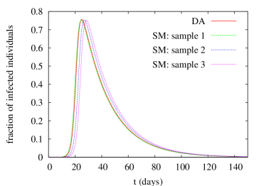
(a)

(b)

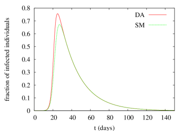
(c)

(d)

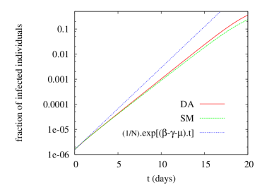
(e)

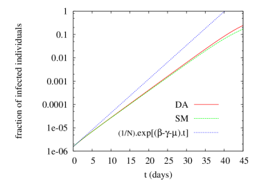
(f)

Figure 1: Fraction of infected individuals as a function of time (t) during the epidemic spread for $p=0.4$. (a) Comparison of DA result with SM simulations for pertussis. For SM three different samples obtained with the same initial condition and different stochastic evolutions are shown; (b) the same as (a) for rubella; (c) comparison of DA result with the mean value function of SM averaged over 5,000 samples for pertussis; (d) the same as (c) for rubella; (e) initial growth of the epidemic for pertussis (detail of figure (c)); (f) initial growth of the epidemic for rubella (detail of figure (d)).

In order to characterize this behavior as a function of $p$, we notice that in this exponential regime the time dependence of the fraction of infected individuals may be written as $c.\exp[(\beta_{exp}-\gamma-\mu)t]$. That is to say, the same as in the classical SIR model (with only global contacts) but with an effective contact rate, $\beta_{exp}$, that is different from $\beta$ because of the presence of local contacts.

It is possible to obtain an analytical approximate expression to estimate $\beta_{exp}$ using DA equations as follows. At the beginning of epidemic growth, when $X_{i}\ll 1$, we have that $X_{r}$ , $X_{si}$ and $X_{sr}$ are also $\ll 1$. So, we drop all the second order terms in $X_{i},X_{r},X_{si}$ and $X_{sr}$, and also the terms $X_{ii},X_{rr},X_{ir}$. As $X_{s}=1-X_{i}-X_{r}$, we may write the 2nd equation of system (6):

$$\frac{dX_{i}}{dt}\simeq-\gamma X_{i}-\mu X_{i}+p\beta X_{i}+\frac{q\beta X_{si}}{4}$$ (7)

If $X_{i}(t)$ presents an exponential behavior, $dX_{i}/dt$ should be proportional to $X_{i}$, so, we assume that in this exponential regime: $X_{si}\simeq KX_{i}$, $K$ being a constant. Expression (7) may now be written as:

$$\frac{dX_{i}}{dt}\simeq-\gamma X_{i}-\mu X_{i}+\left(p+\frac{qK}{4}\right)\beta X_{i}$$ (8)

where $(p+qK/4)\beta$ plays the same rol as $\beta$ in the exponential growth when only global contacts are present. So, we define $\beta^{DA}_{exp}=(p+qK/4)\beta$.

Taking $X_{si}\simeq KX_{i}$ and replacing it in the 2nd and 5th equations of system (6), we may obtain the value of $K$ and compute:

$$\beta^{DA}_{exp}\simeq\frac{1}{4}\left(1+p+\sqrt{1+10p-7p^{2}}\right)\beta$$ (9)

An interesting point here is that, at this level of approximation, DA predicts that $\beta^{DA}_{exp}/\beta$ only depends on $p$ and not on the other parameters characterizing the disease transmission. In Fig.2 we plot this relation for DA (from eq.(9)) and for SM (obtained from exponential fits for different $p$-values) for pertussis and rubella. The agreement between DA and SM is good, but it becomes worse for lower values of $p$. However, even for $p=0.2$ (when the agreement of SM and DA values for $\beta_{exp}$ is not so good) $\beta^{SM}_{exp}/\beta$ accurately verifies the DA prediction of being dependent only on $p$ for pertussis and rubella.

Figure 2: Comparison of SM and DA predictions for the exponential growth regime in an epidemic as a function of $p$. The computation of $\beta^{DA}_{exp}/\beta$ is performed through expression 9 for DA. For SM, $\beta^{SM}_{exp}$ is obtained by fitting the exponential regime of the curve obtained for the average fraction of infected individuals as a function of time to $c\exp[(\beta^{SM}_{exp}-\gamma-\mu)t]$ for each case, where $c$ is a constant.

4.2 Stationary behavior

For the SM presented in Section 2 and a finite value of $N$, the only fixed point (stationary equilibrium) corresponds to the case where all the individuals on the lattice are susceptible. For the stochastic nature of the system, sooner or later a fluctuation leads the number of infected individuals to zero and there is no process that produces new infected people if there are none. But for large values of $N$ (as the one taken in the present study) the system may fluctuate for a long time around a quasi-stationary state (QSS) before extinction. The definition and properties of such a state have been addressed in other contexts from a mathematical point of view [17, 18] or with empirical approaches [19, 20]. In the present work we adopt the empirical strategy developed in ref.[13] where the QSS of the same SM defined in Section 2 is studied. We define a time window ($t_{a},t_{b}$) and generate (for each system studied) more than 20,000 independent samples keeping those that do not become extinct before $t_{b}$. We compute the averages of susceptible and infected individuals over the surviving samples and observe that in the ($t_{a},t_{b}$) interval they remain constant in time within a given precision. We take $t_{a}$=20,000 days and $t_{b}$=40000 days; with these values the considered averages are independent of the initial conditions (as $t_{a}$ is large enough so that correlations in the system may be established) and enough statistics is obtained to compute averages with a relative precision of 0.01. (For details of the definition of the QSS and characterization of the fluctuations for the pertussis case see ref.[13].)

In the case of DA, stationary values are defined as the values of the variables that make all the derivatives in equations (6) zero. They were obtained numerically solving the equations from a given initial condition, X₀, until X$(t)$ is constant in time with a precision 0.00001. For X₀ we take for $X_{s},X_{i}$ and $X_{r}$ the values corresponding to the stationary solution of the SIR model and complete the remainding values of X₀ as in the uncorrelated case. For example, $X_{si}$ is initialized as $4X_{s}X_{i}$ because it is twice the probability that a given pair is of type $SI$ whose value is $2X_{s}X_{i}$ in the uncorrelated case.

In Fig.3a and b we compare the DA stationary values obtained for the fractions of susceptible and infected individuals for pertussis and rubella with the values of these observables averaged over the samples in the QSS of SM. Results for both diseases show an excellent agreement between SM and DA. In Fig.3c we make the same comparison for the fraction of $SI$ pairs on the lattice. The agreement is remarkable considering that this is a correlated quantity directly involved in the DA to SM.

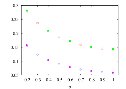
(a)

(b)

(c)

Figure 3: Comparison of DA and SM results for the stationary behavior. (a) Fraction of susceptible individuals; (b) fraction of infected individuals, and (c) fraction of $SI$ pairs on the lattice. Circles correspond to pertussis and squares to rubella. Empty symbols correspond to DA calculations and filled symbols to the estimated average magnitudes in SM.

4.3 System response to a change in $p$

We here study the ability of DA to describe the system response to a sudden change in the globality of the contacts represented in the model by the parameter $p$. We simulate disease transmission at the endemic state in a city where, at a given time, infective contacts among people change and become more local. Such a change could occur because of several circumstances that affect social activities. For example, in Argentina, during the 2009 pandemic flu, the authorities took preventive measures that included suspension of classes at school in July. The population was advised to stay at home whenever possible and to avoid crowded places. These measures aimed at reducing the possibility of an epidemic outbreak during the winter. Our purpose here is to simulate the consequence that this sudden reduction in globality of the contacts may have on the disease transmission of other infectious diseases that are at the endemic state.

We perform simulations with SM for parameters corresponding to pertussis in the prevaccine era and $p=0.5$. Once the QSS is stablished, at a given time (t=20,000 days) we change the value of $p$ to 0.4, which corresponds to a 20% reduction in the globality of contacts. In Fig.4a we compare the dynamic evolution of the system for three samples obtained from SM simulations and DA result. To obtain the DA curve we take the X corresponding to the stationary state for $p$=0.5 as initial condition and at $t=20,000$ we change the value of $p$ to 0.4.

We observe that DA captures the fall down in the fraction of infected individuals after lowering $p$ and the pronounced peaks observed in the following years. The perturbation at $t=20,000$ days puts in phase the oscillations for the different samples that become out of phase again from the third peak. DA also accurately reproduces the time elapsed between peaks. Oscilations are exponentially damped out in DA until the new stationary value is reached. In the case of SM, fluctuations may be very different from sample to sample [13], but as we have seen in Section 4.2, once the QSS is reached, the fraction of infected individuals oscilates around a value very similar to that predicted by DA.

We repeated this study for the case that the system is initially at the QSS corresponding to $p=0.6$ and at $t=20,000$ $p$ is changed to 0.4. In this case, although the final state is the same, the change in the globality of contacts is 33%. In Fig.4b it can be seen that after the perturbation, the system reaches a deep minimum followed by pronounced maxima much higher than in the previous case when the change in $p$ was 20%. Again, DA gives a good description of the observed effects. In this case, most of the samples obtained from the SM simulations become extinct when the system is at the first and pronounced minimum. This is not surprising and could be inferred from the DA result that predicts the number of infected individuals to be below 15 in the time interval (20,400, 20,800 days) for the population considered here. Extinctions in the SM simulations are thus expected, given the fluctuations in the number of infected individuals observed in the dynamic behavior of the system.

(a)

(b)

Figure 4: Time evolution of the fraction of infected individuals for pertussis when a sudden reduction in global contacts occurs. (a) Comparison of DA result with SM simulations when the $p$ parameter is changed from 0.5 to 0.4 at $t=20,000$ days. Initially the system is at the QSS for SM and at stationarity for DA. (b) The same as figure (a) but $p$ is changed from 0.6 to 0.4. In this case, the three samples shown for SM are representative of the ones that survive in the time window shown in the figure. The survival samples in this case represent a fraction of 20% from all the generated samples.

It is worth mentioning that a dynamic behavior similar to that observed in Fig.4 has been found in a recent study of pertussis transmission performed with an age-structured deterministic model with nine epidemiological classes [21]. In that work, the authors proposed that a sudden change in contact rates among individuals could cause a dynamic effect with the presence of deep valleys followed by sharp maxima such as those recently observed in some US states. Here we obtained a similar behavior for the disease transmission as a consequence of having reduced the degree of globality of the contacts in a much more simple epidemiological model.

5 Conclusions

In this work we propose a deterministic approach (DA) for an SIR-type epidemiological model that includes global and local contacts on a square lattice. When comparing our DA with simulations performed with the stochastic version of the model (SM), we obtained a very good agreement for qualitatively different scenarios of disease transmission and parameters corresponding to pertussis and rubella in the prevaccine era.

It would be very valuable to increase the complexity of the model used in the present work in order to study pertussis transmission in the vaccine era. The introduction of pertussis vaccination in the model forces one to include new epidemiological classes that account for individuals that have partially (or totally) lost their immunity [5, 7] as it is well known that immunity to pertussis is not lifelong [22]. We expect the good description obtained with DA for SM to hold if a model with additional epidemiological classes is considered, since the DA to SM involves bassically the description of local contacts that has shown to work very well in different dynamical situations. Stochastic simulations for a more complex model could be much more time-consuming and DA might be the only possible approach to the problem.

6 References

References

- [1] R.M. Anderson and R.M. May. “Infectious diseases of humans: dynamics and control” (Oxford University Press, Oxford, 1991).
- [2] M.J. Keeling and P. Rohani. “Modeling Infectious Diseases in Humans and Animals” (Princeton University Press, Princeton, 2008).
- [3] Hans Heesterbeek, et al. Science 347, aaa4339 (2015). DOI:10.1126/science.aaa4339
- [4] W.O. Kermack and A.G. McKendrick. Proc. Roy. Soc. Lond. A 115, 700 (1927).
- [5] H.W.Hethcote. Math. Biosciences 145, 89 (1997); ibid. 158, 47 (1999).
- [6] R.M. Granich, Ch.F. Gilks, Ch. Dye, K.M. De Cock and B.G. Williams. Lancet 373, 48 (2009)
- [7] G.Fabricius, P.Bergero, M.Ormazabal, A.Maltz and D. Hozbor. Epidemiology and Infection 141, 718 (2013).
- [8] M.S. Bartlett. Proc. Third Berkeley Symp. on Math. Statist. and Prob. 4 (Univ. of Calif. Press, 1956), 81.
- [9] P. Rohani, D. Earn and B.T. Grenfell. Science 286, 968 (1999).
- [10] J. Joo and J. Lebowitz. Phys. Rev E 70 036114 (2004).
- [11] J. Verdasca, M.M. Telo da Gama, A. Nunes, N.R. Bernardino, J.M. Pacheco and M.C. Gomes. Journal of Theoretical Biology 233, 553 (2005).
- [12] M Simöes, M.M. Telo da Gama and A. Nunes. J.R. Soc. Interface 5, 555 (2008).
- [13] M. Dottori and G. Fabricius. Physica A 434, 25 (2015).
- [14] D.T.Gillespie. J. of Comput. Phys. 22, 403 (1976).
- [15] G. Rozhnova and A. Nunes. J. R. Soc. Interface 9, 2959 (2012).
- [16] M. J. Keeling, P. Rohani and B. T. Grenfell. Physica D 148, 317 (2001).
- [17] J.N. Darroch and E. Seneta. Journal of Applied Probability 4, 192 (1967)
- [18] I. Nssel. J. R. Statist. Soc. B 61, 309 (1999)
- [19] M. Martins de Oliveira and R. Dickman. Phys. Rev. E 71, 016129 (2005).
- [20] J. Blanchet, P.W. Glynn and S. Zheng. EVOLVE - A Bridge between Probability, Set Oriented Numerics, and Evolutionary Computation II (Advances in Intelligent Systems and Computing Vol. 175), 19 (2012).
- [21] P. Pesco, P.Bergero, G. Fabricius and D. Hozbor. Epidemics 7, 13 (2014).
- [22] A.M. Wendelboe, A. Van Rie, S. Salmaso and J.A. Englund. The Pediatric Infect. Dis. Journal 24, S58 (2005).