Magnetic-field control of near-field radiative heat transfer and the realization of highly tunable hyperbolic thermal emitters

Abstract

We present a comprehensive theoretical study of the magnetic field dependence of the near-field radiative heat transfer (NFRHT) between two parallel plates. We show that when the plates are made of doped semiconductors, the near-field thermal radiation can be severely affected by the application of a static magnetic field. We find that irrespective of its direction, the presence of a magnetic field reduces the radiative heat conductance, and dramatic reductions up to 700% can be found with fields of about 6 T at room temperature. We show that this striking behavior is due to the fact that the magnetic field radically changes the nature of the NFRHT. The field not only affects the electromagnetic surface waves (both plasmons and phonon polaritons) that normally dominate the near-field radiation in doped semiconductors, but it also induces hyperbolic modes that progressively dominate the heat transfer as the field increases. In particular, we show that when the field is perpendicular to the plates, the semiconductors become ideal hyperbolic near-field emitters. More importantly, by changing the magnetic field, the system can be continuously tuned from a situation where the surface waves dominate the heat transfer to a situation where hyperbolic modes completely govern the near-field thermal radiation. We show that this high tunability can be achieved with accessible magnetic fields and very common materials like $n$-doped InSb or Si. Our study paves the way for an active control of NFRHT and it opens the possibility to study unique hyperbolic thermal emitters without the need to resort to complicated metamaterials.

I Introduction

Radiative heat transfer is a topic with numerous fundamental and technological implications across disciplines Siegel2002 . Presently, the investigation of radiative heat transfer between closely spaced objects is receiving a great attention Zhang2007 ; Joulain2005 ; Volokitin2007 ; Basu2009 ; Song2015a . The basic challenges now are the understanding of the mechanisms governing thermal radiation at the nanoscale and the ability to control this radiation for its use in novel applications. During a long time, it was believed that the maximum radiative heat transfer between two objects was set by the Stefan-Boltzmann law for black bodies. However, this is only true when objects are separated by distances larger than the thermal wavelength (9.6 $\mu$m at room temperature) and the radiative heat transfer is dominated by propagating waves. When two objects are brought in closer proximity, the thermal radiation is dominated by interference effects and, more importantly, by the near field emerging from the materials surfaces in the form of evanescent waves. This was first established theoretically by Polder and Van Hove in 1971 Polder1971 using Rytov’s framework of fluctuational electrodynamics Rytov1953 ; Rytov1989 . These researchers predicted that the NFRHT could overcome the black body limit by several orders of magnitude, achieving what is referred to as super-Planckian thermal emission. Although this NFRHT enhancement was already hinted in several experiments in the late 1960’s Hargreaves1969 ; Domoto1970 , its unambiguous confirmation came only in recent years Kittel2005 ; Narayanaswamy2008 ; Hu2008 ; Rousseau2009 ; Shen2009 ; Ottens2011 ; Shen2012 ; Kralik2012 ; Zwol2012a ; Zwol2012b ; Guha2012 ; Shi2013 ; Worbes2013 ; St-Gelais2014 ; Song2015b ; Lim2015 . These experiments, in turn, have triggered off the hope that NFRHT may have an impact in different technologies such as heat-assisted magnetic recording Challener2009 ; Stipe2010 , thermal lithography Pendry1999 , scanning thermal microscopy Wilde2006 ; Kittel2008 ; Jones2013 , coherent thermal sources Carminati1999 ; Greffet2002 , near-field based thermal management Otey2010 ; Rodriguez2011 ; Guha2012 ; Ben-Abdallah2014 , thermophotovoltaics Messina2013 ; Lenert2014 and other energy conversion devices Schwede2010 .

Presently, one of the central research lines in the field of radiative heat transfer is the search for materials where the NFRHT enhancement can be further increased. So far, the largest enhancements have been experimentally reported in polar dielectrics Rousseau2009 ; Shen2009 ; Song2015b , where the near-field thermal radiation is dominated by the excitation of surface phonon polaritons (SPhPs) Mulet2002 . Similar enhancements have been predicted and observed in doped semiconductors due to surface plasmon polaritons (SPPs) Fu2006 ; Rousseau2009b ; Shi2013 ; Lim2015 . Recently, it has been predicted that hyperbolic metamaterials could behave as broadband super-Planckian thermal emitters Nefedov2011 ; Biehs2012 ; Guo2012 . Hyperbolic metamaterials are a special class of highly anisotropic media that have hyperbolic dispersion. In particular, they are uniaxial materials for which one of the principal components of either the permittivity or the permeability tensors is opposite in sign to the other two principal components Smith2003 . Hyperbolic media have been mainly realized by means of hybrid metal-dielectric superlattices and metallic nanowires embedded in a dielectric host Poddubny2013 ; Shekhar2014 . It has been demonstrated that these metamaterials exhibit exotic optical properties such as negative refraction, subwavelength imaging and focusing, and they can be used to do density of states engineering Poddubny2013 ; Shekhar2014 . In the context of radiative heat transfer, what makes these metamaterials so special is the fact that they can support electromagnetic modes that are evanescent in a vacuum gap, but they are propagating inside the material. This leads to a broadband enhancement of transmission efficiency of the evanescent modes Biehs2012 . This special property has motivated a lot of theoretical work on the use of hyperbolic metamaterials for NFRHT Biehs2013 ; Tschikin2013 ; Guo2013 ; Simovski2013 ; Liu2013 ; Liu2014 ; Guo2014 ; Miller2014 ; Lang2014 ; Nefedov2014 ; Tschikin2015 . However, no experimental investigation of this issue has been reported so far, which is mainly due to the difficulties in handling these metamaterials. In this sense, it would be highly desirable to find much simpler realizations of hyperbolic thermal emitters and, ideally, with tunable properties.

Another key issue in the field of radiative heat transfer is the active control and modulation of NFRHT. In this respect, several proposals have been put forward recently. One of the them is based on the use of phase-change materials Zwol2011a ; Zwol2011b , where the change of phase leads to a significant change in the material dielectric function. These materials include an alloy called AIST, where the phase change can be induced by applying an electric field Zwol2011b , and VO₂, which undergoes a metal-insulator transition as a function of temperature Zwol2011a . It has also been suggested that the NFRHT between chiral materials with magnetoelectric coupling can be tuned by ultrafast optical pulses Cui2012 . Another proposal to tune the NFRHT is to use ferroelectric materials under an external electric field Huang2014 , although the predicted changes are rather modest ($<17$%). Let us also mention that very recently it has been proposed that the heat flux between two semiconductors can be controlled by regulating the chemical potential of photons by means of an external bias Chen2015 . So in short, although these proposals are certainly interesting, some of them are not easy to implement and others are either not very efficient or they are restricted to very specific materials. In this sense, the challenge remains to introduce strategies to actively control NFRHT in an easy and relatively universal way.

In this work we tackle and resolve some of the open problems described above by presenting an extensive theoretical analysis of the influence of an external dc magnetic field in the radiative heat transfer between two parallel plates made of a variety of materials. We show that an applied magnetic field can indeed largely affect the NFRHT in a broad class of materials, namely doped (polar and non-polar) semiconductors. We find that, irrespective of its orientation, the magnetic field reduces the NFRHT with respect to the zero-field case and we show that the reduction can be as large as 700% for fields of about 6 T at room temperature. This effect originates from the fact that the magnetic field not only strongly modifies the surface waves that dominate the NFRHT in doped semiconductors (both SPhPs and SPPs), but it also generates broadband hyperbolic modes that tend to govern the heat transfer as the field is increased. In particular, when the applied field is perpendicular to the plates surfaces, the semiconductors behave as hyperbolic thermal emitters with highly tunable properties. By changing the field magnitude one can continuously tune the system and realize situations where (i) surface waves dominate the NFRHT, (ii) both surface waves and hyperbolic modes contribute significantly to the near-field thermal radiation, and (iii) only hyperbolic modes contribute to the NFRHT and surface waves cease to exist. On the other hand, when the field is parallel to the surfaces the NFRHT is nonmonotonic as a function of the magnetic field. For moderate fields, surface waves and hyperbolic modes coexisting, while for high fields the NFRHT is largely dominated by hyperbolic modes. We emphasize that all these striking predictions are amenable to measurements and do not require the use of any complicated metamaterial. Thus, our work offers a simple strategy to actively control NFRHT in a broad variety of materials and it also provides a very appealing recipe to realize hyperbolic materials and, in particular, hyperbolic thermal emitters with highly tunable properties.

The remainder of this paper is structured as follows. Section II describes the system under study and the general formalism for the description of NFRHT in the presence of a magnetic field. We then turn in Sec. III to the application of the general results to the case of $n$-doped InSb as an example of a polar semiconductor. We discuss in this section both the results for different magnetic field orientations and the realization of highly tunable hyperbolic thermal emitters. Section III is devoted to the case of Si as an example of non-polar semiconductor. Section IV summarizes our main results and discusses future directions. Finally, four appendixes contain the technical details of the general formalism and some additional calculations that support the claims in this paper.

II Radiative heat transfer in the presence of a magnetic field: General formalism

Our main goal is to compute the radiative heat transfer in the presence of an external dc magnetic field within the framework of fluctuational electrodynamics Rytov1953 ; Rytov1989 . For simplicity, we shall concentrate here in the heat exchanged between two infinite parallel plates made of arbitrary non-magnetic materials and that are separated by a vacuum gap of width $d$, see Fig. 1(a). The magnetic field can point in any direction and following Fig. 1(a), we shall refer to the left plate as medium 1, the vacuum gap as medium 2, and the right plate as medium 3.

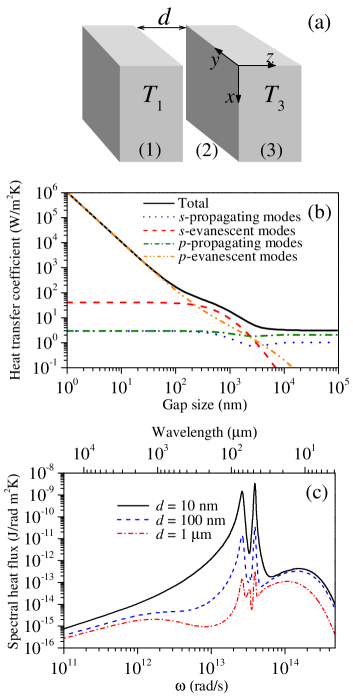
Figure 1: (a) Schematic representation of the system under study: two parallel plates at temperatures $T_{1}$ and $T_{3}$ separated by a vacuum gap of width $d$. (b) Heat transfer coefficient of $n$-doped InSb as a function of the gap at zero magnetic field. We show the total result and the individual contributions of $s$- and $p$-polarized waves (both propagating and evanescent). (c) The corresponding zero-field spectral heat flux as a function of frequency (and wavelength) for three different gaps.

When a magnetic field is applied to any object, it results in an optical anisotropy that can be described by the following general permittivity tensor Zvezdin1997

$$\hat{\epsilon}=\left(\begin{array}[]{ccc}\epsilon_{xx}&\epsilon_{xy}&\epsilon_{xz}\\ \epsilon_{yx}&\epsilon_{yy}&\epsilon_{yz}\\ \epsilon_{zx}&\epsilon_{zy}&\epsilon_{zz}\end{array}\right),$$ (1)

where according to Fig. 1(a), $x$ and $y$ lie in the interface planes and $z$ corresponds to the surface normal. The components of the permittivity tensor depend on the applied magnetic field, as we shall specify below, and on the frequency (local approximation). Let us recall that the off-diagonal elements in Eq. (1) are responsible for all the well-known magneto-optical effects (Faraday effect, Kerr effects, etc.) Zvezdin1997 . Thus, our problem is to compute the radiative heat transfer between two anisotropic parallel plates. This generic problem has been addressed by Biehs et al. Biehs2011 and we just recall here the central result. The net power per unit of area exchanged between the parallel plates is given by the following Landauer-like expression Biehs2011

$$Q=\int^{\infty}_{0}\frac{d\omega}{2\pi}\left[\Theta_{1}(\omega)-\Theta_{3}(\omega)\right]\int\frac{d{\bf k}}{(2\pi)^{2}}\tau(\omega,{\bf k},d),$$ (2)

where $\Theta_{i}(\omega)=\hbar\omega/[\exp(\hbar\omega/k_{\rm B}T_{i})-1]$, $T_{i}$ is the absolute temperature of the layer $i$, $\omega$ is the radiation frequency, ${\bf k}=(k_{x},k_{y})$ is the wave vector parallel to the surface planes, and $\tau(\omega,{\bf k},d)$ is the total transmission probability of the electromagnetic waves. Notice that the second integral in Eq. (2) is carried out over all possible directions of ${\bf k}$ and it includes the contribution of both propagating waves with $k<\omega/c$ and evanescent waves with $k>\omega/c$, where $k$ is the magnitude of ${\bf k}$ and $c$ is the velocity of light in vacuum. The transmission coefficient $\tau(\omega,{\bf k},d)$ can be expressed as Biehs2011

$$\tau(\omega,{\bf k},d)=\hskip 199.16928pt$$ (3)

$$\left\{\begin{array}[]{ll}\mbox{Tr}\left\{[\hat{1}-\hat{\cal R}_{21}\hat{\cal R}^{\dagger}_{21}]\hat{\cal D}^{\dagger}[\hat{1}-\hat{\cal R}^{\dagger}_{23}\hat{\cal R}_{23}]\hat{\cal D}\right\},&k<\omega/c\\ \mbox{Tr}\left\{[\hat{\cal R}_{21}-\hat{\cal R}^{\dagger}_{21}]\hat{\cal D}^{\dagger}[\hat{\cal R}^{\dagger}_{23}-\hat{\cal R}_{23}]\hat{\cal D}\right\}e^{-2|q_{2}|d},&k>\omega/c\end{array}\right.,$$ (6)

where $q_{2}=\sqrt{\omega^{2}/c^{2}-k^{2}}$ is the $z$-component of the wave vector in the vacuum gap and the $2\times 2$ matrices $\hat{\cal R}_{ij}$ are the reflections matrices characterizing the two interfaces. These matrices have the following generic structure

$$\hat{\cal R}_{ij}=\left(\begin{array}[]{cc}r^{s,s}_{ij}&r^{s,p}_{ij}\\ r^{p,s}_{ij}&r^{p,p}_{ij}\end{array}\right),$$ (7)

where $r^{\alpha,\beta}_{ij}$ with $\alpha,\beta=s,p$ is the reflection amplitude for the scattering of an incoming $\alpha$-polarized plane wave into an outgoing $\beta$-polarized wave. Finally, the $2\times 2$ matrix $\hat{\cal D}$ appearing in Eq. (3) is defined as

$$\hat{\cal D}=[\hat{1}-\hat{\cal R}_{21}\hat{\cal R}_{23}e^{2iq_{2}d}]^{-1}.$$ (8)

Notice that this matrix describes the usual Fabry-Pérot-like denominator resulting from the multiple scattering between the two interfaces.

In Appendixes A and B we provide an alternative derivation of the central result of Eq. (3) that emphasizes the non-reciprocal nature of our problem. More importantly, we show explicitly how the different reflection matrices appearing in Eq. (3) can be computed within a scattering-matrix approach for anisotropic multilayer systems. This approach provides, in turn, a natural framework to analyze different issues that will be crucial later on such as the nature of the electromagnetic modes responsible for the heat transfer.

The result of Eqs. (2) and (3) reduces to the well-known result for isotropic media first derived by Polder and Van Hove Polder1971 . In that case, the reflections matrices of Eq. (7) are diagonal and the non-vanishing elements are given by

$$r^{s,s}_{ij} = \frac{q_{i}-q_{j}}{q_{i}+q_{j}}$$ (9)

$$r^{p,p}_{ij} = \frac{\epsilon_{j}q_{i}-\epsilon_{i}q_{j}}{\epsilon_{j}q_{i}+\epsilon_{i}q_{j}},$$ (10)

where $q_{i}=\sqrt{\epsilon_{i}\omega^{2}/c^{2}-k^{2}}$ is the transverse or $z$-component of the wave vector in layer $i$ and $\epsilon_{i}(\omega)$ is the corresponding dielectric constant. Thus, the total transmission can be written as $\tau(\omega,{\bf k},d)=\tau_{s}(\omega,{\bf k},d)+\tau_{p}(\omega,{\bf k},d)$, where the contributions of $s$- and $p$-polarized waves are given by

$$\tau_{\alpha=s,p}(\omega,{\bf k},d)=\hskip 170.71652pt$$ (11)

$$\left\{\begin{array}[]{ll}(1-|r^{\alpha,\alpha}_{21}|^{2})(1-|r^{\alpha,\alpha}_{23}|^{2})/|D_{\alpha}|^{2},\;\;k<\omega/c\\ 4\mbox{Im}\{r^{\alpha,\alpha}_{21}\}\mbox{Im}\{r^{\alpha,\alpha}_{23}\}e^{-2|q_{2}|d}/|D_{\alpha}|^{2},\;\;k>\omega/c\end{array}\right.,$$ (14)

where $D_{\alpha}=1-r^{\alpha,\alpha}_{21}r^{\alpha,\alpha}_{23}e^{2iq_{2}d}$. Throughout this work we focus on the analysis of the radiative linear heat conductance per unit of area, $h$, which is referred to as the heat transfer coefficient. This coefficient is given by

$$h(T,d)=\lim_{\Delta T\rightarrow 0^{+}}\frac{Q(T_{1}=T+\Delta T,T_{3}=T,d)}{\Delta T},$$ (15)

where $T$ is the absolute temperature that we assume equal to 300 K throughout this work. Additionally, we define the spectral heat flux as the heat transfer coefficient per unit of frequency. In the following sections, we apply the general results presented here to different materials and magnetic field configurations.

III Polar semiconductors: InSb

The first obvious question to be answered is: In which materials can a magnetic field modify the NFRHT? Since the thermal radiation of an object is primarily determined by its dielectric function, we need materials in which this function can be modified by an external magnetic field, that is we need magneto-optical (MO) materials. Focusing on room temperature experiments, the MO activity must be exhibited in the mid-infrared. Thus, doped semiconductors, where the MO activity is due to conduction electrons, are ideal candidates Kushwaha2001 . In these materials, one can play with the doping level to tune the plasma frequency to values comparable to the cyclotron frequency at experimentally achievable magnetic fields, which is an important requirement to have sizable magnetic-induced effects in the NFRHT (see discussion below). Moreover, in semiconductors the NFRHT in the absence of field is typically dominated by surface electromagnetic waves (both SPhPs and SPPs), which in turn are known to be strongly influenced by an external magnetic field Kushwaha2001 ; Wallis1982 . Thus, it seems natural to expect a magnetic-field modulation of NFRHT in semiconductors.

There is a variety of semiconductors that we could choose to illustrate our predictions. In this section we focus on InSb for several reasons. First, it is a polar semiconductor where the NFRHT in the absence of field is dominated by two different types of surface waves (SPhPs and SPPs), which allows us to study a very rich phenomenology. Second, InSb has a small effective mass, which enables to tune the cyclotron frequency to values comparable to those of the plasma frequency with moderate fields. Finally, InSb has been the most widely studied material in the context of magnetoplasmons and coupled magnetoplasmons-surface phonon polaritons. Thus, the magnetic field effect in the surface waves has been very well characterized experimentally Palik1973 ; Hartstein1975 ; Palik1976 ; Remer1984 .

III.1 Perpendicular magnetic field: The realization of hyperbolic near-field thermal emitters

Let us first discuss the radiative heat transfer between two identical plates made of $n$-doped InSb when the magnetic field is perpendicular to the plate surfaces, i.e. ${\bf H}=H_{z}\hat{\bf z}$, see Fig. 1(a). In this case, the permittivity tensor of InSb adopts the following form Palik1976

$$\hat{\epsilon}(H)=\left(\begin{array}[]{ccc}\epsilon_{1}(H)&-i\epsilon_{2}(H)&0\\ i\epsilon_{2}(H)&\epsilon_{1}(H)&0\\ 0&0&\epsilon_{3}\end{array}\right),$$ (16)

where

$$\epsilon_{1}(H) = \epsilon_{\infty}\left(1+\frac{\omega^{2}_{L}-\omega^{2}_{T}}{\omega^{2}_{T}-\omega^{2}-i\Gamma\omega}+\frac{\omega^{2}_{p}(\omega+i\gamma)}{\omega[\omega^{2}_{c}-(\omega+i\gamma)^{2}]}\right),$$

$$\epsilon_{2}(H) = \frac{\epsilon_{\infty}\omega^{2}_{p}\omega_{c}}{\omega[(\omega+i\gamma)^{2}-\omega^{2}_{c}]},$$ (17)

$$\epsilon_{3} = \epsilon_{\infty}\left(1+\frac{\omega^{2}_{L}-\omega^{2}_{T}}{\omega^{2}_{T}-\omega^{2}-i\Gamma\omega}-\frac{\omega^{2}_{p}}{\omega(\omega+i\gamma)}\right).$$

Here, $\epsilon_{\infty}$ is the high-frequency dielectric constant, $\omega_{L}$ is the longitudinal optical phonon frequency, $\omega_{T}$ is the transverse optical phonon frequency, $\omega^{2}_{p}=ne^{2}/(m^{\ast}\epsilon_{0}\epsilon_{\infty})$ defines the plasma frequency of free carriers of density $n$ and effective mass $m^{\ast}$, $\Gamma$ is the phonon damping constant, and $\gamma$ is the free-carrier damping constant. Finally, the magnetic field enters in these expressions via the cyclotron frequency $\omega_{c}=eH/m^{\ast}$. The important features of the previous expressions are: (i) the magnetic field induces an optical anisotropy (via the modification of the diagonal elements and the introduction of off-diagonal ones), (ii) there are two major contributions to the diagonal components of the dielectric tensor: optical phonons and free carriers, and (iii) the MO activity is introduced via the free carriers, which illustrates the need to deal with doped semiconductors. In what follows we shall concentrate in a particular case taken from Ref. [Palik1976, ], where $\epsilon_{\infty}=15.7$, $\omega_{L}=3.62\times 10^{13}$ rad/s, $\omega_{T}=3.39\times 10^{13}$ rad/s, $\Gamma=5.65\times 10^{11}$ rad/s, $\gamma=3.39\times 10^{12}$ rad/s, $n=1.07\times 10^{17}$ cm^-3, $m^{\ast}/m=0.022$, and $\omega_{p}=3.14\times 10^{13}$ rad/s. As a reference, let us say that with these parameters $\omega_{c}=8.02\times 10^{12}$ rad/s for a field of 1 T. Let us point out that in this configuration, and due to the structure of the permittivity tensor, the transmission coefficient appearing in Eq. (2) only depends on the magnitude of the parallel wave vector, which considerably simplifies the calculation of the radiative heat transfer.

Let us now briefly review the expectations for the heat transfer in the absence of magnetic field. As we show in Fig. 1(b), the heat transfer coefficient features a large near-field enhancement for gaps below 1 $\mu$m. For $d<100$ nm this enhancement is largely dominated by $p$-polarized evanescent waves and the heat transfer coefficient increases as $1/d^{2}$ as the gap decreases, which are two clear signatures of a situation where the heat transfer is dominated by surface electromagnetic waves. This can be further confirmed with the analysis of the spectral heat flux, see Fig. 1(c), which in the near-field regime is dominated by two narrow peaks that can be associated to SPPs (low-frequency peak) and SPhPs (high-frequency peak), as it will become evident below. Thus, the case of InSb constitutes an interesting example where two types of surface waves contribute significantly to the NFRHT. Let us now see how these results are modified in the presence of a magnetic field.

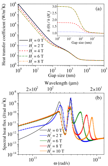
Figure 2: (a) Heat transfer coefficient for $n$-doped InSb as a function of the gap for different values of the magnetic field perpendicular to the plate surfaces. The inset shows the ratio between the zero-field coefficient and the coefficient for different values of the field in the near-field region. (b) The corresponding spectral heat flux as a function of the frequency (and wavelength) for a gap of $d=10$ nm and different values of the perpendicular field. The solid lines correspond to the exact calculation and the circles to the uniaxial approximation where the off-diagonal terms of the permittivity tensor are assumed to be zero.

In Fig. 2(a) we show the heat transfer coefficient as a function of the gap size for different values of the perpendicular magnetic field. There are three salient features: (i) the far-field heat transfer is fairly independent of the magnetic field, (ii) in the near-field regime (below 300 nm) the magnetic field suppresses the heat transfer by up to a factor of 3 (see inset), and (iii) by increasing the field, the heat transfer coefficient tends to saturate at around 6 T, although it is slightly reduced upon further increasing the field above 10 T (not shown here). The strong modification of heat transfer due to the magnetic field is even more apparent in the spectral heat flux. As one can see in Fig. 2(b), the magnetic field not only distorts and reduces the height of the peaks related to the surface waves, but it also generates a new peak that shifts to higher frequencies as the field increases. This additional peak appears at the cyclotron frequency and its presence illustrates the high tunability that can be achieved. Notice, for instance, that for a field of 6 T the thermal emission at the cyclotron frequency is increased by almost 3 orders of magnitude with respect to the zero-field case.

To shed more light on these results it is convenient to examine the transmission of the $p$-polarized waves, which can be shown to dominate the heat transfer for any field. We present in Fig. 3 this transmission as a function of the magnitude of the parallel wave vector, $k$, and the frequency for a gap $d=10$ nm and different values of the magnetic field. As one can see, at low fields the transmission maxima are located around a restricted area of $k$ and $\omega$, clearly indicating that surface waves dominate the NFRHT. Notice also that their dispersion relation is modified by the field, see Fig. 3(b). By increasing the field, those areas are progressively replaced by areas where the maximum transmission is reached for a broad range of $k$-values and finally, the surface waves are restricted to the reststrahlen band $\omega_{T}<\omega<\omega_{L}$ for the highest fields, see Fig. 3(d). What is the nature of these magnetic-field-induced modes?

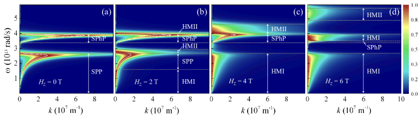
Figure 3: The transmission coefficient for $p$-polarized waves as a function of the magnitude of the parallel wave vector and frequency for InSb and a gap of $d=10$ nm. The different panels correspond to different values of the magnetic field that is perpendicular to the surfaces. The horizontal dashed lines separate the regions where transmission is dominated by surface waves (SPPs and SPhPs) or hyperbolic modes of type I and II (HMI and HMII). The white solid lines correspond to the analytical dispersion relation of the surface waves of Eq. (18).

To answer this question and explain all the results just described, it is important to realize that the off-diagonal elements of the permittivity tensor do not play a major role in this configuration. This is illustrated in Fig. 2(b) where we show that the approximation consisting in setting $\epsilon_{2}=0$ in Eq. (16) reproduces very accurately the exact results for the spectral heat flux for arbitrary magnetic fields. This means that the polarization conversion is irrelevant and the plates effectively behave as uniaxial media where their permittivity tensors are diagonal: $\hat{\epsilon}=$ diag$[\epsilon_{xx},\epsilon_{xx},\epsilon_{zz}]$, where $\epsilon_{xx}=\epsilon_{1}$ and $\epsilon_{zz}=\epsilon_{3}$. Within this approximation, which hereafter we refer to as uniaxial approximation, it is easy to compute the dispersion relation of the surface electromagnetic modes in our geometry (see Appendix D). In the electrostatic limit $k\gg\omega/c$, the dispersion relation of these cavity modes is given by

$$k_{\rm SW}=\frac{1}{d}\ln\left(\pm\frac{\epsilon_{xx}-\sqrt{\epsilon_{xx}/\epsilon_{zz}}}{\epsilon_{xx}+\sqrt{\epsilon_{xx}/\epsilon_{zz}}}\right),$$ (18)

with the additional constraint that both $\epsilon_{xx}$ and $\epsilon_{zz}$ must be negative. In the zero-field limit, this expression reduces to the known result for cavity surface modes in isotropic materials Song2015b . As we show in Fig. 3, see white solid lines, the dispersion relation of Eq. (18) nicely reproduces the structure of the transmission maxima in those frequency regions in which surfaces waves are allowed ($\epsilon_{xx},\epsilon_{zz}<0$). It is worth stressing that this dispersion relation describes in a unified manner both the SPPs that appear below the reststrahlen band and the SPhPs due to the optical phonons. More importantly, this dispersion relation tells us that the magnetic field reduces the parallel wave vector of the surface waves and restricts the frequency region where they exist. Indeed, at high fields the SPPs disappear, while the SPhPs are restricted to the reststrahlen band, Fig. 3(d). These two effects are actually the cause of the reduction of the NFRHT in the presence of a magnetic field. But what about the other modes that appear by increasing the field? Their nature can also be understood within the uniaxial approximation. As we show in Appendix C, the allowed values for the transverse component of the wave vector inside these uniaxial materials are given by $q_{\rm o}=\sqrt{\epsilon_{xx}\omega^{2}/c^{2}-k^{2}}$ for ordinary waves and $q_{\rm e}=\sqrt{\epsilon_{xx}\omega^{2}/c^{2}-k^{2}\epsilon_{xx}/\epsilon_{zz}}$ for extraordinary waves. The dispersion of the extraordinary waves can be rewritten as

$$\frac{k^{2}_{x}+k^{2}_{y}}{\epsilon_{zz}}+\frac{q^{2}_{\rm e}}{\epsilon_{xx}}=\frac{\omega^{2}}{c^{2}},$$ (19)

a dispersion that becomes hyperbolic when $\epsilon_{xx}$ and $\epsilon_{zz}$ have opposite signs Smith2003 . This is exactly what happens in our case in certain frequency regions at finite field. This illustrated in Fig. 3(b-d), where we have indicated the hyperbolic regions defined by the condition $\epsilon_{xx}\epsilon_{zz}<0$. Notice that those regions correspond exactly to the areas where the transmission reaches its maximum for a broad range of $k$-values. This fact shows unambiguously that our InSb plates effectively behave as hyperbolic materials. More importantly, and as it is evident from Fig. 3, we can easily modify the hyperbolic regions by changing the field. Thus, we can change from situations where the hyperbolic modes (HMs) coexist with both types of surface waves to situations where the HMs dominate the NFRHT, which is what occurs at high fields, see Fig. 3(d). Moreover, contrary to what happens in most hybrid hyperbolic metamaterials, we can have in a single material HMs of type I (HMI), where $\epsilon_{xx}>0$ and $\epsilon_{zz}<0$, and HMs of type II (HMII), where $\epsilon_{xx}<0$ and $\epsilon_{zz}>0$, see Fig. 3(b-d).

Let us recall that what makes HMs so special in the context of NFRHT is the fact that, as it is evident from their dispersion relation, they are evanescent in the vacuum gap and propagating inside the hyperbolic material for $k>\omega/c$ (HMI) or $k>\sqrt{|\epsilon_{zz}|}\omega/c$ (HMII). Thus, they are a special kind of frustrated internal reflection modes that exhibit a very high transmission over a broad range of $k$-values that correspond to evanescent waves in the vacuum gap Biehs2012 . As shown in Ref. [Biehs2012, ], the number of HMs that contributes to the NFRHT is solely determined by the intrinsic cutoff in the transmission, which has the form $\tau(\omega,k)\propto\exp(-2kd)$ for $k\gg\omega/c$. From this condition it follows that the heat flux due to HMs scales as $1/d^{2}$ for small gaps, as the contribution of surface waves. This explains why the appearance of HMs as the field increases does not modify the parametric dependence of the NFRHT with the gap size. Notice, however, that in spite of the high transmission of these HMs, their appearance does not enhance the NFRHT because they replace surface waves that possess even larger $k$-values (notice that the conditions of HMs and surface waves are mutually excluding). Thus, we can conclude that the NFRHT reduction induced by the magnetic field is due to both the modification of the surface waves and their replacement by HMs that, in spite of their propagating nature inside the material, turn out to be less efficient transferring the radiative heat in the near-field region than the surface waves.

Let us point out that within the uniaxial approximation, the heat transfer can be obtained in a semi-analytical form. In this case, the transmission coefficient is given by the isotropic result of Eq. (11), where the reflections coefficients adopt now the form

$$r^{s,s}_{21}=r^{s,s}_{23} = \frac{q_{2}-q_{\rm o}}{q_{2}+q_{\rm o}}$$ (20)

$$r^{p,p}_{21}=r^{p,p}_{23} = \frac{\epsilon_{xx}q_{2}-q_{\rm e}}{\epsilon_{xx}q_{2}+q_{\rm e}}.$$ (21)

The uniaxial approximation is also useful to understand the high field behavior of the NFRHT. The tendency to saturate the thermal radiation as the field increases is due to the to the fact that the cyclotron frequency becomes larger than the plasma frequency and the last term in the expression of $\epsilon_{xx}=\epsilon_{1}$, see Eq. (17), progressively becomes more irrelevant. Thus, the permittivity tensor becomes field-independent and the heat transfer is simply given by the result for uniaxial media, where $\epsilon_{zz}=\epsilon_{3}$ has the form in Eq. (17), but $\epsilon_{xx}=\epsilon_{1}$ does not contain the last term in the first expression of Eq. (17). We find that the strict saturation of the NFRHT occurs at around 20 T and there is an intermediate regime, between 6 and 20 T, in which the near-field thermal radiation slightly increases upon increasing the field (not shown here), leading to a nonmonotonic behavior. This behavior is due to an increase in the efficiency of the HMs that dominate the NFRHT in this high-field regime.

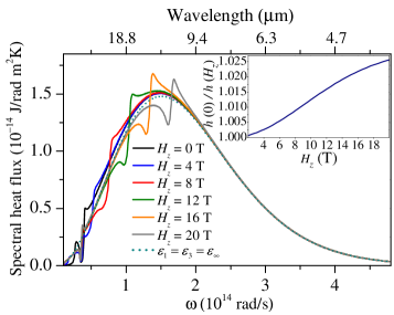
Figure 4: Far-field spectral heat flux for InSb as a function of the frequency (and wavelength) for different values of the perpendicular field. These spectra have been computed for a gap $d=1$ m. The dotted line corresponds to the result for plates made of a dielectric with a frequency-independent dielectric constant equal to $\epsilon_{\infty}$. The inset shows the corresponding ratio between the zero-field heat transfer coefficient and the coefficient for different values of the field.

To conclude this subsection, let us explain why the far-field heat transfer is rather insensitive to the magnetic field. For gaps much larger than the thermal wavelength ($9.6\;\mu$m), the heat transfer is dominated by propagating waves and, as we show in Fig. 4, the spectral heat flux in the absence of field exhibits a broad spectrum with a peak at around $1.5\times 10^{14}$ rad/s. Indeed, the spectrum is very similar to that of a dielectric with a frequency-independent dielectric constant $\hat{\epsilon}=\epsilon_{\infty}\hat{1}$, see dotted line in Fig. 4. As we illustrate in that figure, the presence of a magnetic field only modifies this spectrum in a significant way in a small region around the cyclotron frequency. This fact leads to a tiny modification of the heat transfer upon the application of an external field. As it can be seen in the inset of Fig. 4, the magnetic field reduces the far-field heat transfer coefficient as the magnetic field increases, but this reduction is quite modest and, for instance, it amounts to only 2.5% at a very high field of 20 T.

III.2 Parallel magnetic field

Let us now turn to the case in which the magnetic field is parallel to the plate surfaces. For concreteness, we consider that the field is applied along the $x$-axis, ${\bf H}=H_{x}\hat{\bf x}$, but obviously the result is independent of the field direction as long as it points along the surface plane, as we have explicitly checked. In this case, the permittivity tensor of InSb adopts the form

$$\hat{\epsilon}(H)=\left(\begin{array}[]{ccc}\epsilon_{3}&0&0\\ 0&\epsilon_{1}(H)&-i\epsilon_{2}\\ 0&i\epsilon_{2}(H)&\epsilon_{1}(H)\end{array}\right),$$ (22)

where the $\epsilon$’s are given by Eq. (17). Let us emphasize that in this case the transmission coefficient appearing in Eq. (2) depends both on the magnitude of the parallel wave and on its direction, which makes the calculations more demanding. Let us also say that we consider here the same parameter values for the $n$-doped InSb as in the example analyzed above.

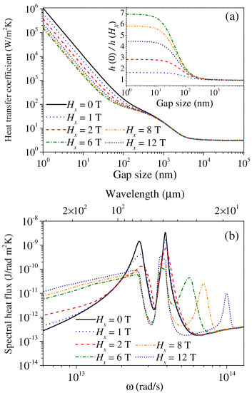
Figure 5: (a) Heat transfer coefficient for $n$-doped InSb as a function of the gap for different values of the magnetic field applied along the surfaces of the plates. The inset shows the ratio between the zero-field coefficient and the coefficient for different values of the field in the near-field region. (b) The corresponding spectral heat flux as a function of the frequency (and wavelength) for a gap of $d=10$ nm and different values of the parallel field.

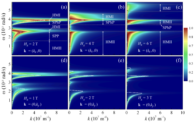
Figure 6: The transmission coefficient for $p$-polarized waves as a function of the magnitude of the parallel wave vector and frequency for InSb and a gap of $d=10$ nm. In all cases the field is parallel to the plate surfaces, ${\bf H}=H_{x}\hat{\bf x}$. The panels (a-c) correspond to different values of the magnetic field for wave vectors parallel to field, ${\bf k}=(k_{x},0)$, while panels (d-f) correspond to wave vectors perpendicular to the field, ${\bf k}=(0,k_{y})$. The horizontal dashed lines separate the regions where transmission is dominated by surface waves (SPPs and SPhPs) or hyperbolic modes of type I and II (HMI and HMII). The white solid lines correspond to the analytical dispersion relation of the surface waves of Eq. (18) in panels (a-c) and of Eq. (23) in panels (d-f).

The results for the magnetic field dependence of the heat transfer coefficient for the parallel configuration are summarized in Fig. 5(a). As in the perpendicular case, the far-field is barely affected by the magnetic field, the near-field thermal radiation is suppressed by the field, and at high fields the NFRHT tends to saturates. Interestingly, it saturates to the same value as in the perpendicular configuration. In spite of the similarities, there are also important differences. In this case, the NFRHT is much more sensitive to the field and a significant reduction is already achieved at 1 T. Notice also that in this case the heat transfer coefficient is clearly nonmonotonic and the maximum reduction is reached at around 6 T. Finally, notice also that the reduction is more pronounced than in the perpendicular case and the NFRHT can be diminished by up to a factor of 7 with respect to the zero-field case, see inset of Fig. 5(a). This more pronounced reduction in the parallel configuration is also apparent in the spectral heat flux, as one can see in Fig. 5(b). Notice that also in this case there appears a high-frequency peak that is blue-shifted as the field increases. This peak appears at the cyclotron frequency and it has the same origin as in the perpendicular case.

Again, to understand this complex phenomenology, it is convenient to examine the transmission of the $p$-polarized waves, which dominate the NFRHT for any field. Since in this case the transmission also depends on the direction of k, we choose to analyze the two most representative directions. In the first one, the in-plane wave vector ${\bf k}$ is parallel to the field, i.e. ${\bf k}=(k_{x},0)$, and in the second one, ${\bf k}$ is perpendicular to the field, i.e. ${\bf k}=(0,k_{y})$. The transmission of $p$-polarized waves for these two directions is shown in Fig. 6 as a function of the magnitude of the wave vector and as a function of the frequency for different values of the field. As one can see, the transmission exhibits very different behaviors for these two directions. While for ${\bf k}\parallel{\bf H}$ the situation resembles that of a perpendicular field (see discussion above), for ${\bf k}\perp{\bf H}$ it seems like the transmission is dominated by surface waves that are severely affected by the magnetic field (with the appearance of gaps in their dispersion relations). These very different behaviors can be understood with an analysis of both the surface waves and the propagating waves inside the material in these two situations. In the case ${\bf k}\parallel{\bf H}$, one can show that a uniaxial approximation, similar to that discussed above, accurately reproduces the results for the transmission found in the exact calculation. In this case, the permittivity tensor can be approximated by $\hat{\epsilon}=$ diag$[\epsilon_{xx},\epsilon_{zz},\epsilon_{zz}]$, where $\epsilon_{xx}=\epsilon_{3}$ and $\epsilon_{zz}=\epsilon_{1}$. Within this approximation, the dispersion relation of surface waves in the electrostatic limit $k\gg\omega/c$ is also given by Eq. (18) (see Appendix D). As we show in Fig. 6(a-c), this dispersion relation nicely describes the structure of the transmission maxima in the regions where the surface waves can exist ($\epsilon_{xx},\epsilon_{zz}<0$). On the other hand, as we show in Appendix C, the allowed values for the transverse component of the wave vector inside these uniaxial-like materials are given by $q_{\rm o}=\sqrt{\epsilon_{zz}\omega^{2}/c^{2}-k^{2}}$ for ordinary waves and $q_{\rm e}=\sqrt{\epsilon_{xx}\omega^{2}/c^{2}-k^{2}\epsilon_{xx}/\epsilon_{zz}}$ for extraordinary waves. Again, the dispersion of these extraordinary waves is of hyperbolic type when $\epsilon_{xx}$ and $\epsilon_{zz}$ have opposite signs. In Fig. 6(a-c) we identify the frequency regions where the HMs exist with the condition $\epsilon_{xx}\epsilon_{zz}<0$, regions that progressively dominate the transmission as the field increases. Thus, we see that for ${\bf k}\parallel{\bf H}$ the situation is very similar to that extensively discussed in the case in which the field is perpendicular to the materials’ surfaces.

On the contrary, the situation is very different for ${\bf k}\perp{\bf H}$. In this case, there are no HMs and no uniaxial approximation can describe the situation. As we show in Appendix C, the allowed $q$-values are given by $q_{\rm o,1}=\sqrt{\epsilon_{xx}\omega^{2}/c^{2}-k^{2}}$ and $q_{\rm o,2}=\sqrt{(\epsilon^{2}_{yy}+\epsilon^{2}_{yz})\omega^{2}/(c^{2}\epsilon_{yy})-k^{2}}$, which both describe waves with no hyperbolic dispersion. On the other hand, the dispersion relation of the surface waves in the electrostatic limit is given by

$$k_{\rm SW}=\frac{1}{2d}\ln\left(\frac{(\eta_{yy}-1+i\eta_{yz})(\eta_{yy}-1-i\eta_{yz})}{(\eta_{yy}+1+i\eta_{yz})(\eta_{yy}+1-i\eta_{yz})}\right),$$ (23)

where $\eta_{yy}=\epsilon_{yy}/(\epsilon_{yy}^{2}+\epsilon_{yz}^{2})$ and $\eta_{yz}=-\epsilon_{yz}/(\epsilon_{yy}^{2}+\epsilon_{yz}^{2})$. As we show in Fig. 6(d-f), this dispersion relation explains the complex structure of the transmission maxima in this case. We emphasize that this dispersion relation is reciprocal in our symmetric geometry and for this reason we only show results for $k_{y}>0$. Notice that this dispersion is very sensitive to the magnetic field and already fields of the order of 1 T strongly affect the surface waves. Notice also the appearance of gaps in the dispersion relations, a subject that has been extensively discussed in the case of a single interface Kushwaha2001 ; Wallis1982 . Overall, the field rapidly reduces the $k$-values of the surface waves and restricts the regions where they can exist. This strong sensitivity of the surface waves with ${\bf k}\perp{\bf H}$ is the reason for the more pronounced reduction of the NFRHT for this field configuration.

In general, for an arbitrary direction ${\bf k}=(k_{x},k_{y})$ the situation is somehow a combination of the two types of behaviors just described. The complex interplay of these behaviors for different ${\bf k}$-directions is responsible for the nonmonotonic dependence with magnetic field, along with the change in efficiency of the HMs upon varying the field. On the other hand, at very high fields the cyclotron frequency becomes much larger than the plasma frequency and the off-diagonal elements of the permittivity tensor become negligible. At the same time, the field-dependent terms in the diagonal elements also become very small. Thus, the systems effectively become uniaxial and field-independent and the heat transfer is identical to the case in which the field is perpendicular. Finally, in the far-field regime, the heat transfer is not sensitive to the magnetic field for the same reason as in the perpendicular configuration.

Let us conclude this section with two brief comments. First, as it is obvious from the discussions above, another way to modulate the NFRHT is by rotating the magnetic field, while keeping fixed its magnitude. Actually, we find that for any field magnitude, the NFRHT is always smaller in the parallel configuration. Thus, one can increase or decrease the near-field thermal radiation by rotating appropriately the magnetic field. Second, we have focused here in the case of doped InSb, but similar results can in principle be obtained for other doped polar semiconductors such as GaAs, InAs, InP, PbTe, SiC, etc.

IV Non-polar semiconductors: Si

In the previous section we have seen that when the field is parallel to the surfaces, one can have hyperbolic emitters, but the HMs always coexist to some degree with surface waves (even at the highest field). We show in this section that in the case of non-polar semiconductors, where phonons do not play any role, it is possible to tune the system with a magnetic field to a situation where only HMs contribute to the NFRHT. For this purpose, we choose Si as the material for the two plates. As mentioned in the introduction, it has been predicted Fu2006 ; Rousseau2009b , and experimentally tested Shi2013 ; Lim2015 , that in doped Si the NFRHT in the absence of field can be dominated by SPPs even at room temperature. Let us see now how this is modified upon applying a magnetic field.

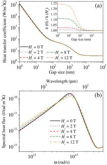
Figure 7: (a) Heat transfer coefficient for $n$-doped Si as a function of the gap for different values of the magnetic field perpendicular to the plate surfaces. The inset shows the ratio between the zero-field coefficient and the coefficient for different values of the field in the near-field region. (b) The corresponding spectral heat flux as a function of the frequency (and wavelength) for a gap of $d=10$ nm.

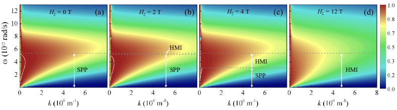
Figure 8: The transmission coefficient for $p$-polarized waves as a function of the magnitude of the parallel wave vector and frequency for Si and a gap of $d=10$ nm. The different panels correspond to different values of the magnetic field that is perpendicular to the surfaces. The horizontal dashed lines separate the regions where transmission is dominated by surface plasmon polaritons (SPPs) or hyperbolic modes of type I (HMI). The white solid lines correspond to the analytical SPP dispersion relation of Eq. (18).

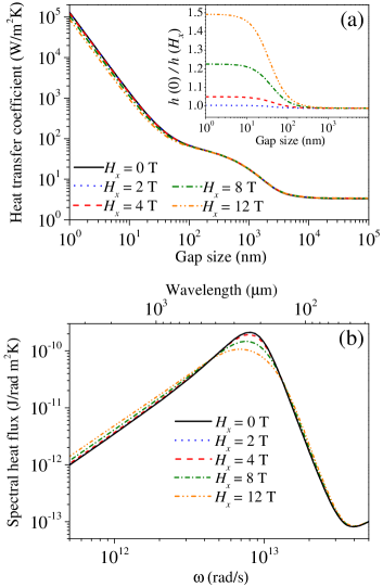
Figure 9: (a) Heat transfer coefficient for $n$-doped Si as a function of the gap for different values of the magnetic field applied along the surfaces of the plates. The inset shows the ratio between the zero-field coefficient and the coefficient for different values of the field in the near-field region. (b) The corresponding spectral heat flux as a function of the frequency (and wavelength) for a gap of $d=10$ nm.

The dielectric properties of doped Si are similar to those of InSb, the only difference being the absence of a phonon contribution. Thus, the dielectric functions of Eq. (17) now read

$$\epsilon_{1}(H) = \epsilon_{\infty}\left(1+\frac{\omega^{2}_{p}(\omega+i\gamma)}{\omega[\omega^{2}_{c}-(\omega+i\gamma)^{2}]}\right),$$

$$\epsilon_{3} = \epsilon_{\infty}\left(1-\frac{\omega^{2}_{p}}{\omega(\omega+i\gamma)}\right),$$ (24)

while $\epsilon_{2}(H)$ remains unchanged. Using the results of Ref. [Fu2006, ] for the dielectric constant of doped Si, we focus on a room temperature case where the electron concentration is $n=9.3\times 10^{16}$ cm^-3, $\epsilon_{\infty}=11.7$, $\gamma=8.04\times 10^{12}$ rad/s, $m^{\ast}/m=0.27$, and $\omega_{p}=9.66\times 10^{12}$ rad/s. We have chosen this doping level to have a situation in which the plasma frequency is not too high so that we can affect the NFRHT with a magnetic field, and not too low so that the NFRHT in the absence of field is still dominated by SPPs.

The results for the heat transfer coefficient and spectral heat flux for a perpendicular magnetic field are displayed in Fig. 7. Although there are several features that are similar to those of the InSb case, there are also some notable differences. To begin with, notice that now higher fields are needed to see a significant reduction of the NFRHT (the required fields are around an order of magnitude higher than for InSb) and the reduction factors are clearly more modest, see inset of Fig. 7(a). This is mainly a consequence of the smaller cyclotron frequency in the Si case for a given field due to its larger effective mass. Another consequence of the small cyclotron frequency is the fact that there is no sign of saturation of the NFRHT for reasonable magnetic fields. On the other hand, the spectral heat flux at low fields is dominated this time by a single broad peak that originates from SPPs (see discussion below). As the field increases, the peak height is reduced and the peak itself is broadened and deformed. As we show in what follows, this behavior is due to the appearance of HMs that at high fields completely replace the surface waves.

Again, we can gain a further insight into these results by analyzing the transmission of the $p$-polarized waves for different fields, which is illustrated in Fig. 8. As one can see, the transmission is dominated by evanescent waves (in the vacuum gap) in a frequency region right below the plasma frequency. The origin of the structure of the transmission maxima can be understood with the uniaxial approximation discussed above in the context of InSb. Again, this approximation reproduces very accurately all the results for arbitrary perpendicular fields (not shown here). Within this approximation, one can see that at low fields the transmission is dominated by SPPs, as we illustrate in Fig. 8(a-b) in which we have introduced the dispersion relation of the SPPs given by Eq. (18). As soon as the magnetic magnetic field becomes finite, the system starts to develop HMs of type I in a tiny frequency region right above the region of existence of the SPPs, see Fig. 8(b). The origin of these HMs is identical to that of the InSb case, but the main difference in this case is that upon increasing the field, one reaches a critical field value (of 4.36 T for this example) for which the surface waves cease to exist and the transmission is completely dominated by HMs turning the Si plates into “pure” hyperbolic thermal emitters, see Fig. 8(c-d).

For completeness, we have also studied the heat transfer in the parallel configuration and the results for the heat transfer coefficient and spectral heat flux are shown in Fig. 9. In this case the results are rather similar to those of the perpendicular configuration. In particular, contrary to the InSb case we do not find a nonmonotonic behavior. Moreover, the NFRHT reduction is not much more pronounced than in the perpendicular case, although one can reach reduction factors of 50% for 12 T. Finally, saturation is not reached for these high fields for the same reason as in the perpendicular configuration. As in the case of InSb, all these results can be understood in terms of the modes that govern the near-field thermal radiation. In this sense, for a direction where ${\bf k}\parallel{\bf H}$, the SPPs that dominate the NFRHT at low fields are progressively replaced by HMIs upon increasing the field and above 4.36 T they “eat out” all surface waves. On the contrary, for ${\bf k}\perp{\bf H}$ there are no HMs and the only magnetic field effect is the modification of the SPP dispersion relation. Again, the interplay between these two characteristic behaviors among the different ${\bf k}$-directions explains the evolution of the NFRHT with the field.

Let us conclude this section by saying that the behavior reported here for Si could also be observed for other non-polar semiconductors such as Ge.

V Outlook and conclusions

The results reported in this work raise numerous interesting questions. Thus for instance, in all cases analyzed so far, we have found that the magnetic field reduces the NFRHT as compared to the zero-field result. Is there any fundamental argument that forbids a magnetic-field-induced enhancement? In principle, there is no such an argument. The reduction that we have found in doped semiconductors is due to the fact that the we have explored cases where surface waves, which are extremely efficient, dominate the NFRHT in the absence of field. In this sense, one may wonder if a field-induced enhancement could take place in a situation where the NFRHT in the absence of field is dominated by standard frustrated internal reflection modes, as it happens in metals Chapuis2008 . Obviously, metals are out of the question due to their huge plasma frequency, but one can investigate non-polar semiconductors with a low doping level. Indeed, we have done it for the case of Si and again, we find that the magnetic field reduces the NFRHT and moreover, exceedingly high fields are required to see any significant effect. Of course, we have by no means exhausted all possibilities and, for instance, we have not explored asymmetric situations with different materials. Thus, the question remains of whether the application of a magnetic field can under certain circumstances enhance the near-field thermal radiation.

The discovery in this work of the induction of hyperbolic modes upon the application of a magnetic field may also have important consequences for layered structures involving thin films. Recently, it has been demonstrated that thin films made of polar dielectrics may support NFRHT enhancements comparable to those of bulk samples due to the excitation of SPhPs Song2015b . Since hyperbolic modes have a propagating character inside the material, they may be severely affected in a thin film geometry by the presence of a substrate. Thus, one could expect much more dramatic magnetic-field effects in systems coated with semiconductor thin films.

Obviously, the question remains of whether one can modulate the NFRHT with a magnetic field in other classes of materials. For instance, since a magneto-optical activity is required, what about ferromagnetic materials? Ideally, one could imagine to tune the NFRHT by playing around with the relative orientation of the magnetization, following the spin-valve experiments in the context of spintronics.

Another question of general interest for the field of metamaterials is if a doped semiconductor under a magnetic field could exhibit the plethora of exotic optical properties reported in hybrid hyperbolic metamaterials Poddubny2013 ; Shekhar2014 . We have shown here that it can behave as a hyperbolic thermal emitter, but can it also exhibit negative refraction or be used do to subwavelength imaging and focusing in the infrared? These are very important questions that we are currently pursuing.

So in summary, we have presented in this work a very detailed theoretical analysis of the influence of a magnetic field in the NFRHT. By considering the simple case of two parallel plates, we have demonstrated that for doped semiconductors the near-field thermal radiation can be strongly modified by the application of an external magnetic field. In particular, we have shown that the magnetic field may significantly reduce the NFRHT and the reduction in polar semiconductors can be as large as 700% at room temperature. Moreover, we have shown that when the field is perpendicular to the parallel plates, doped semiconductors become ideal hyperbolic thermal emitters with highly tunable properties. This provides a unique opportunity to explore the physics of thermal radiation in this class of metamaterials without the need to resort to complex hybrid structures. Finally, all the predictions of this work are amenable to measurements with the present experimental techniques, and we are convinced that the multiple open questions that this work raises will motivate many new theoretical and experimental studies of this subject.

Appendix A Scattering matrix approach for anisotropic multilayer systems

Our analysis of the radiative heat transfer in the presence of a static magnetic field is based on the combination of Rytov’s fluctuational electrodynamics (FE) and a scattering matrix formalism that describes the propagation of electromagnetic waves in multilayer systems made of optically anisotropic materials. As we show in Appendix B, the radiative heat transfer can be expressed in terms of the scattering matrix of our system. Thus, it is convenient to first discuss in this appendix the scattering matrix approach employed in this work ignoring for the moment the fluctuating currents that generate the thermal radiation. Later in Appendix B, we show how this approach can be combined with FE. We follow here Ref. [Caballero2012, ], which presents a generalization of the formalism introduced by Whittaker and Culshaw in Ref. [Whittaker1999, ] for isotropic systems.

Let us first describe the Maxwell’s equations to be solved. Assuming a harmonic time dependence $\exp(-i\omega t)$, the Maxwell’s equations for non-magnetic materials and in the absence of currents adopt the following form: ${\bf\nabla}\cdot\epsilon_{0}\hat{\epsilon}{\bf E}=0$, ${\bf\nabla}\cdot{\bf H}=0$, ${\bf\nabla}\times{\bf H}=-i\omega\epsilon_{0}\hat{\epsilon}{\bf E}$, and ${\bf\nabla}\times{\bf E}=i\omega\mu_{0}{\bf H}$, where the permittivity is in general a tensor given by Eq. (1). The first Maxwell’s equation is automatically satisfied if the third one is fulfilled, and the second one can be satisfied by expanding the magnetic field in terms of basis functions with zero divergence. Following Ref. [Whittaker1999, ], it is convenient to introduce the rescaling: $\omega\epsilon_{0}{\bf E}\to{\bf E}$ and $\sqrt{\mu_{0}\epsilon_{0}}\omega=\omega/c\to\omega$. Thus, the final two equations to be solved are

$${\bf\nabla}\times{\bf H} = -i\hat{\epsilon}{\bf E},$$ (25)

$${\bf\nabla}\times{\bf E} = i\omega^{2}{\bf H}.$$ (26)

We consider here a planar multilayer system grown along the $z$-direction in which the tensor $\hat{\epsilon}$ is constant inside every layer, i.e. it is independent of the in-plane coordinates ${\bf r}\equiv(x,y)$. Thus, for an in-plane wave vector ${\bf k}\equiv(k_{x},k_{y})$, we can write the fields as

$${\bf H}({\bf r},z)=\bm{h}(z)e^{i{\bf k}\cdot{\bf r}}\;\;\mbox{and}\;\;{\bf E}({\bf r},z)=\bm{e}(z)e^{i{\bf k}\cdot{\bf r}}.$$ (27)

With this notation, Eqs. (25) and (26) can be rewritten as

$$ik_{y}h_{z}(z)-h^{\prime}_{y}(z) = -i\sum_{j}\epsilon_{xj}e_{j}(z)$$ (28)

$$h^{\prime}_{x}(z)-ik_{x}h_{z}(z) = -i\sum_{j}\epsilon_{yj}e_{j}(z)$$ (29)

$$ik_{x}h_{y}(z)-ik_{y}h_{x}(z) = -i\sum_{j}\epsilon_{zj}e_{j}(z),$$ (30)

and

$$ik_{y}e_{z}(z)-e^{\prime}_{y}(z) = i\omega^{2}h_{x}(z)$$ (31)

$$e^{\prime}_{x}(z)-ik_{x}e_{z}(z) = i\omega^{2}h_{y}(z)$$ (32)

$$ik_{x}e_{y}(z)-ik_{y}e_{x}(z) = i\omega^{2}h_{z}(z),$$ (33)

where the primes stand for $\partial_{z}$.

Now our task is to solve the Maxwell’s equations for an unbounded layer. For this purpose, we write the magnetic field $\bm{h}(z)$ as follows

$$\bm{h}(z)=e^{iqz}\left\{\phi_{x}{\bf\hat{x}}+\phi_{y}{\bf\hat{y}}-\frac{1}{q}(k_{x}\phi_{x}+k_{y}\phi_{y}){\bf\hat{z}}\right\},$$ (34)

where ${\bf\hat{x}}$, ${\bf\hat{y}}$, and ${\bf\hat{z}}$ are the Cartesian unit vectors and $q$ is the $z$-component of the wave vector. Here, $\phi_{x}$ and $\phi_{y}$ are the expansion coefficients to be determined by substituting into Maxwell’s equations. Notice that this expression satisfies ${\bf\nabla}\cdot{\bf H}=0$. Now, it is convenient to rewrite the previous expression in the vector notation:

$$\bm{h}(z)=e^{iqz}\left(\phi_{x},\phi_{y},-\frac{1}{q}(k_{x}\phi_{x}+k_{y}\phi_{y})\right)^{T}.$$ (35)

With this notation, Eqs. (28-30) can be written as

$$\hat{\cal C}\bm{h}(z)=\hat{\epsilon}\bm{e}(z),\;\;\mbox{where}\;\;\hat{\cal C}=\left(\begin{array}[]{ccc}0&q&-k_{y}\\ -q&0&k_{x}\\ k_{y}&-k_{x}&0\end{array}\right).$$ (36)

On the other hand, Eqs. (31-33) adopt now the form

$$\hat{\cal C}^{T}\bm{e}(z)=\omega^{2}\bm{h}(z).$$ (37)

From Eq. (36) we obtain the following expression for the electric field

$$\bm{e}(z)=\hat{\eta}\hat{\cal C}\bm{h}(z),$$ (38)

where $\hat{\eta}=\hat{\epsilon}^{-1}$. Substituting this expression in Eq. (37) we obtain the following equation for the magnetic field

$$\hat{\cal C}^{T}\hat{\eta}\hat{\cal C}\bm{h}(z)=\omega^{2}\bm{h}(z),$$ (39)

which defines an eigenvalue problem for $\omega^{2}$. Indeed, only two of the three identities obtained from this equation, one for each ${\bf\hat{x}}$, ${\bf\hat{y}}$, and ${\bf\hat{z}}$, are independent. From the first two identities, and using Eq. (35), we obtain the following equations determining the allowed values for $q$

$$\left(\hat{\cal A}_{2}q^{2}+\hat{\cal A}_{1}q+\hat{\cal A}_{0}+\hat{\cal A}_{-1}\frac{1}{q}\right)\phi=0,$$ (40)

where $\phi=(\phi_{x},\phi_{y})^{T}$ and the $2\times 2$ matrices $\hat{\cal A}_{n}$ are defined by

$$\hat{\cal A}_{2}=\left(\begin{array}[]{cc}\eta_{yy}&-\eta_{yx}\\ -\eta_{xy}&\eta_{xx}\end{array}\right),\;\;\hat{\cal A}_{1}=\hat{\cal A}^{(a)}_{1}+\hat{\cal A}^{(b)}_{1}=\left(\begin{array}[]{cc}-k_{y}\eta_{zy}&k_{y}\eta_{zx}\\ k_{x}\eta_{zy}&-k_{x}\eta_{zx}\end{array}\right)+\left(\begin{array}[]{cc}-k_{y}\eta_{yz}&k_{x}\eta_{yz}\\ k_{y}\eta_{xz}&-k_{x}\eta_{xz}\end{array}\right),$$ (47)

$$\hat{\cal A}_{0}=\hat{\cal A}^{(a)}_{0}+\hat{\cal A}^{(b)}_{0}-\omega^{2}\hat{1}=\left(\begin{array}[]{cc}k^{2}_{y}\eta_{zz}&-k_{x}k_{y}\eta_{zz}\\ -k_{x}k_{y}\eta_{zz}&k^{2}_{x}\eta_{zz}\end{array}\right)+\left(\begin{array}[]{cc}k^{2}_{x}\eta_{yy}-k_{x}k_{y}\eta_{yx}&k_{x}k_{y}\eta_{yy}-k^{2}_{y}\eta_{yx}\\ k_{x}k_{y}\eta_{xx}-k^{2}_{x}\eta_{xy}&k^{2}_{y}\eta_{xx}-k_{x}k_{y}\eta_{xy}\end{array}\right)-\omega^{2}\left(\begin{array}[]{cc}1&0\\ 0&1\end{array}\right),$$ (54)

$$\hat{\cal A}_{-1}=\left(\begin{array}[]{cc}k^{2}_{y}k_{x}\eta_{zx}-k^{2}_{x}k_{y}\eta_{zy}&k^{3}_{y}\eta_{zx}-k^{2}_{y}k_{x}\eta_{zy}\\ k^{3}_{x}\eta_{zy}-k^{2}_{x}k_{y}\eta_{zx}&k^{2}_{x}k_{y}\eta_{zy}-k^{2}_{y}k_{x}\eta_{zx}\end{array}\right).$$ (57)

This eigenvalue problem leads to the following quartic secular equation: $\sum^{4}_{n=0}D_{n}q^{n}=0$, where the coefficients are given by

$$D_{4} = \eta_{xx}\eta_{yy}-\eta_{xy}\eta_{yx},$$

$$D_{3} = k_{x}\left[\eta_{xy}\eta_{yz}+\eta_{yx}\eta_{zy}-\eta_{yy}(\eta_{xz}+\eta_{zx})\right]+k_{y}\left[\eta_{yx}\eta_{xz}+\eta_{xy}\eta_{zx}-\eta_{xx}(\eta_{yz}+\eta_{zy})\right],$$

$$D_{2} = k^{2}_{x}\left[\eta_{yy}(\eta_{xx}+\eta_{zz})-\eta_{xy}\eta_{yx}-\eta_{yz}\eta_{zy}\right]+k^{2}_{y}\left[\eta_{xx}(\eta_{yy}+\eta_{zz})-\eta_{xy}\eta_{yx}-\eta_{xz}\eta_{zx}\right]$$

$$+k_{x}k_{y}\left[\eta_{xz}(\eta_{yz}+\eta_{zy})+\eta_{yz}(\eta_{zx}-\eta_{xz})\eta_{zz}(\eta_{xy}+\eta_{yx})\right]-\omega^{2}(\eta_{xx}+\eta_{yy}),$$

$$D_{1} = k^{3}_{x}\left[\eta_{xy}\eta_{yz}+\eta_{yx}\eta_{zy}-\eta_{yy}(\eta_{xz}+\eta_{zx})\right]+k^{3}_{y}\left[\eta_{yx}\eta_{xz}+\eta_{xy}\eta_{zx}-\eta_{xx}(\eta_{yz}+\eta_{zy})\right]$$

$$+k^{2}_{x}k_{y}\left[\eta_{xy}\eta_{zx}+\eta_{xz}\eta_{yx}-\eta_{xx}(\eta_{yz}+\eta_{zy})\right]+k^{2}_{y}k_{x}\left[\eta_{yx}\eta_{zy}+\eta_{yz}\eta_{xy}-\eta_{yy}(\eta_{xz}+\eta_{zx})\right]$$

$$+\omega^{2}\left[k^{2}_{x}(\eta_{xz}+\eta_{zx})+k^{2}_{y}(\eta_{yz}+\eta_{zy})\right],$$

$$D_{0} = k^{4}_{x}(\eta_{yy}\eta_{zz}-\eta_{yz}\eta_{zy})+k^{4}_{y}(\eta_{xx}\eta_{zz}-\eta_{xz}\eta_{zx})+k^{3}_{x}k_{y}\left[\eta_{xz}\eta_{zy}+\eta_{yz}\eta_{zx}-\eta_{zz}(\eta_{xy}+\eta_{yx})\right]$$ (58)

$$+k^{3}_{y}k_{x}\left[\eta_{yz}\eta_{zx}+\eta_{xz}\eta_{zy}-\eta_{zz}(\eta_{yx}+\eta_{xy})\right]+k^{2}_{x}k^{2}_{y}\left[\eta_{zz}(\eta_{xx}+\eta_{yy})+\eta_{xy}\eta_{yx}-\eta_{xz}\eta_{zx}-\eta_{yz}\eta_{zy}\right]$$

$$+\omega^{2}\left[\omega^{2}-k^{2}_{x}(\eta_{yy}+\eta_{zz})-k^{2}_{y}(\eta_{xx}+\eta_{zz})+k_{x}k_{y}(\eta_{xy}+\eta_{yx})\right].$$

In general, this secular equation has to be solved numerically, but in many situations of interest the allowed values for $q$ can be obtained analytically (see Appendix C). The solution of Eq. (40) provides four complex eigenvalues for $q$, two lie in the upper half of the complex plane and the other two in the lower half.

The next step toward the solution of the Maxwell’s equations in a multilayer structure is the determination of the fields in the different layers. This can be done by expressing the fields as a combination of forward and backward propagating waves with wave numbers $q_{n}$ (with $n=1,2$), and complex amplitudes $a_{n}$ and $b_{n}$, respectively. These amplitudes will be determined later by using the boundary conditions at the interfaces and surfaces of the multilayer structure. Since the boundary conditions are simply the continuity of the in-plane field components, we focus here on the analysis of the field components $e_{x}$, $e_{y}$, $h_{x}$, and $h_{y}$. From Eq. (35), the in-plane components of $\bm{h}$ can be expanded in terms of propagating waves as follows

$$\left(\begin{array}[]{c}h_{x}(z)\\ h_{y}(z)\end{array}\right) = \sum^{2}_{n=1}\left\{\left(\begin{array}[]{c}\phi_{x_{n}}\\ \phi_{y_{n}}\end{array}\right)e^{iq_{n}z}a_{n}\right.$$ (66)

$$\hskip 14.22636pt\left.+\left(\begin{array}[]{c}\varphi_{x_{n}}\\ \varphi_{y_{n}}\end{array}\right)e^{-ip_{n}(d-z)}b_{n}\right\},$$

where $d$ is the thickness of the layer. Here, $a_{n}$ is the coefficient of the forward going wave at the $z=0$ interface, and $b_{n}$ is the backward going wave at $z=d$. On the other hand, $q_{n}$ correspond to the eigenvalues of Eq. (40) with $\mbox{Im}\{q_{n}\}>0$ and $p_{n}$ are the eigenvalues with $\mbox{Im}\{p_{n}\}<0$.

To simplify the notation, we now define two $2\times 2$ matrices $\hat{\Phi}_{+}$ and $\hat{\Phi}_{-}$ whose columns are the vectors $\phi_{n}$ and $\varphi_{n}$, respectively. Moreover, we define the diagonal $2\times 2$ matrices $\hat{\rm f}_{+}(z)$ and $\hat{\rm f}_{-}(d-z)$, such that $[\hat{\rm f}_{+}(z)]_{nn}=e^{iq_{n}z}$ and $[\hat{\rm f}_{-}(d-z)]_{nn}=e^{-ip_{n}(d-z)}$, and the $2$-dimensional vectors $\bm{h}_{\parallel}(z)=(h_{x}(z),h_{y}(z))^{T}$, $\bm{a}=(a_{1},a_{2})^{T}$, and $\bm{b}=(b_{1},b_{2})^{T}$. In terms of these quantities, the in-plane magnetic-field components become

$$\bm{h}_{\parallel}(z)=\hat{\Phi}_{+}\hat{\rm f}_{+}(z)\bm{a}+\hat{\Phi}_{-}\hat{\rm f}_{-}(d-z)\bm{b}.$$ (67)

Similarly, from Eq. (38) it is straightforward to show that the in-plane components of the electric field, $\bm{e}_{\parallel}(z)=(-e_{y}(z),e_{x}(z))^{T}$, are given by

$$\bm{e}_{\parallel}(z) = \left(\hat{\cal A}^{(b)}_{0}\hat{\Phi}_{+}\hat{q}^{-1}+\hat{\cal A}^{(b)}_{1}\hat{\Phi}_{+}+\hat{\cal A}_{2}\hat{\Phi}_{+}\hat{q}\right)\hat{\rm f}_{+}(z)\bm{a}$$ (68)

$$+\left(\hat{\cal A}^{(b)}_{0}\hat{\Phi}_{-}\hat{p}^{-1}+\hat{\cal A}^{(b)}_{1}\hat{\Phi}_{-}+\hat{\cal A}_{2}\hat{\Phi}_{-}\hat{p}\right)\hat{\rm f}_{-}(d-z)\bm{b},$$

where the $\hat{\cal A}$’s are defined in Eq. (57) and we have defined the $2\times 2$ diagonal matrices $\hat{q}$ and $\hat{p}$ such that $\hat{q}_{nn}=q_{n}$ and $\hat{p}_{nn}=p_{n}$.

We can now combine Eq. (67) and (68) into a single expression as follows

$$\left(\begin{array}[]{c}\bm{e}_{\parallel}(z)\\ \bm{h}_{\parallel}(z)\end{array}\right) = \hat{M}\left(\begin{array}[]{c}\hat{\rm f}_{+}(z)\bm{a}\\ \hat{\rm f}_{-}(d-z)\bm{b}\end{array}\right)$$ (73)

$$= \left(\begin{array}[]{cc}\hat{M}_{11}&\hat{M}_{12}\\ \hat{M}_{21}&\hat{M}_{22}\end{array}\right)\left(\begin{array}[]{c}\hat{\rm f}_{+}(z)\bm{a}\\ \hat{\rm f}_{-}(d-z)\bm{b}\end{array}\right),$$ (78)

where the $2\times 2$ matrices $M_{ij}$ are defined as

$$\hat{M}_{11} = \hat{\cal A}^{(b)}_{0}\hat{\Phi}_{+}\hat{q}^{-1}+\hat{\cal A}^{(b)}_{1}\hat{\Phi}_{+}+\hat{\cal A}_{2}\hat{\Phi}_{+}\hat{q},$$

$$\hat{M}_{12} = \hat{\cal A}^{(b)}_{0}\hat{\Phi}_{-}\hat{p}^{-1}+\hat{\cal A}^{(b)}_{1}\hat{\Phi}_{-}+\hat{\cal A}_{2}\hat{\Phi}_{-}\hat{p},$$

$$\hat{M}_{21} = \hat{\Phi}_{+},\;\;\;\hat{M}_{22}=\hat{\Phi}_{-}.$$ (79)

The final step in our calculation is to use the scattering matrix ($S$-matrix) to compute the field amplitudes needed to describe the different relevant physical quantities. By definition, the $S$-matrix relates the vectors of the amplitudes of forward and backward going waves, $\bm{a}_{l}$ and $\bm{b}_{l}$, where $l$ now denotes the layer, in the different layers of the structure as follows

$$\left(\begin{array}[]{c}\bm{a}_{l}\\ \bm{b}_{l^{\prime}}\end{array}\right)=\hat{S}(l^{\prime},l)\left(\begin{array}[]{c}\bm{a}_{l^{\prime}}\\ \bm{b}_{l}\end{array}\right)=\left(\begin{array}[]{cc}\hat{S}_{11}&\hat{S}_{12}\\ \hat{S}_{21}&\hat{S}_{22}\end{array}\right)\left(\begin{array}[]{c}\bm{a}_{l^{\prime}}\\ \bm{b}_{l}\end{array}\right).$$ (80)

The field amplitudes in two consecutive layers are related via the continuity of the in-plane components of the fields in every interface and surface. If we consider the interface between the layer $l$ and the layer $l+1$, this continuity leads to

$$\left(\begin{array}[]{c}\bm{e}_{\parallel}(d_{l})\\ \bm{h}_{\parallel}(d_{l})\end{array}\right)_{l}=\left(\begin{array}[]{c}\bm{e}_{\parallel}(0)\\ \bm{h}_{\parallel}(0)\end{array}\right)_{l+1},$$ (81)

where $d_{l}$ is the thickness of layer $l$. From this condition, together with Eq. (73), it is easy to show that the amplitudes in layers $l$ and $l+1$ are related by the interface matrix $\hat{I}(l,l+1)=\hat{M}^{-1}_{l}\hat{M}_{l+1}$ in the following way

$$\left(\begin{array}[]{c}\hat{f}^{+}_{l}\bm{a}_{l}\\ \bm{b}_{l}\end{array}\right) = \hat{I}(l,l+1)\left(\begin{array}[]{c}\bm{a}_{l+1}\\ \hat{f}^{-}_{l+1}\bm{b}_{l+1}\end{array}\right)$$ (86)

$$= \left(\begin{array}[]{cc}\hat{I}_{11}&\hat{I}_{12}\\ \hat{I}_{21}&\hat{I}_{22}\end{array}\right)\left(\begin{array}[]{c}\bm{a}_{l+1}\\ \hat{f}^{-}_{l+1}\bm{b}_{l+1}\end{array}\right),$$ (91)

where $\hat{f}^{+}_{l}=\hat{\rm f}_{l,+}(d_{l})$ and $\hat{f}^{-}_{l+1}=\hat{\rm f}_{l+1,-}(d_{l+1})$.

Now, with the help of the interface matrices, the $S$-matrix can be calculated in an iterative way as follows. The matrix $\hat{S}(l^{\prime},l+1)$ can be calculated from $\hat{S}(l^{\prime},l)$ using the definition of $\hat{S}(l^{\prime},l)$ in Eq. (80) and the interface matrix $\hat{I}(l,l+1)$. Eliminating $\bm{a}_{l}$ and $\bm{b}_{l}$ we obtain the relation between $\bm{a}_{l^{\prime}}$, $\bm{b}_{l^{\prime}}$ and $\bm{a}_{l+1}$, $\bm{b}_{l+1}$, from which $\hat{S}(l^{\prime},l+1)$ can be constructed. This reasoning leads to the following iterative relations

$$\hat{S}_{11}(l^{\prime},l+1) = \left[\hat{I}_{11}-\hat{f}^{+}_{l}\hat{S}_{12}(l^{\prime},l)\hat{I}_{21}\right]^{-1}\hat{f}^{+}_{l}\hat{S}_{11}(l^{\prime},l)$$

$$\hat{S}_{12}(l^{\prime},l+1) = \left[\hat{I}_{11}-\hat{f}^{+}_{l}\hat{S}_{12}(l^{\prime},l)\hat{I}_{21}\right]^{-1}$$

$$\times\left(\hat{f}^{+}_{l}\hat{S}_{12}(l^{\prime},l)\hat{I}_{22}-\hat{I}_{12}\right)\hat{f}^{-}_{l+1}$$

$$\hat{S}_{21}(l^{\prime},l+1) = \hat{S}_{22}(l^{\prime},l)\hat{I}_{21}\hat{S}_{11}(l^{\prime},l+1)+\hat{S}_{21}(l^{\prime},l)$$

$$\hat{S}_{22}(l^{\prime},l+1) = \hat{S}_{22}(l^{\prime},l)\hat{I}_{21}\hat{S}_{12}(l^{\prime},l+1)+$$ (92)

$$\hat{S}_{22}(l^{\prime},l)\hat{I}_{22}\hat{f}^{-}_{l+1}.$$

Starting from $\hat{S}(l^{\prime},l^{\prime})=1$, one can apply the previous recursive relations to a layer at a time to build up $\hat{S}(l^{\prime},l)$. Let us conclude this appendix by saying that from the knowledge of the $S$-matrix one can easily compute the field amplitudes in every layer and, in turn, the fields everywhere in the system Whittaker1999 .

Appendix B Thermal radiation in anisotropic multilayer systems

In this appendix we show how the scattering matrix approach of Appendix A can be used to describe the thermal radiation between planar multilayer systems made of anisotropic materials. For this purpose, we first discuss how a generic emission problem can be formulated in the framework of the $S$-matrix formalism and then, we show how such a formulation can be used to describe the thermal emission of a multilayer system.

B.1 Emission in the scattering matrix approach

For concreteness, let us assume that there is a set of oscillating point sources, with harmonic time dependence, occupying the whole plane defined by $z=z^{\prime}$. The corresponding electric current density ${\bf J}$ is given by

$${\bf J}({\bf r},z)={\bf J}_{0}\delta(z-z^{\prime})=\bm{j}_{0}e^{i{\bf k}\cdot{\bf r}}\delta(z-z^{\prime}),$$ (93)

where $\bm{j}_{0}({\bf k})={\bf J}_{0}e^{-i{\bf k}\cdot{\bf r}}$. This current density enters as a source term in Ampère’s law, Eq. (25), which now becomes ${\bf\nabla}\times{\bf H}={\bf J}-i\hat{\epsilon}{\bf E}$, while Eq. (26) (Faraday’s law) remains unchanged. Thus, Eqs. (28-30) adopt now the following form

$$ik_{y}h_{z}(z)-h^{\prime}_{y}(z) = j_{0x}\delta(z-z^{\prime})-i\sum_{j}\epsilon_{xj}e_{j}(z)$$ (94)

$$h^{\prime}_{x}(z)-ik_{x}h_{z}(z) = j_{0y}\delta(z-z^{\prime})-i\sum_{j}\epsilon_{yj}e_{j}(z)$$ (95)

$$ik_{x}h_{y}(z)-ik_{y}h_{x}(z) = j_{0z}\delta(z-z^{\prime})-i\sum_{j}\epsilon_{zj}e_{j}(z).\hskip 19.91684pt$$ (96)

The presence of the source term induces discontinuities in the fields across the plane $z=z^{\prime}$, as we proceed to show. First, let us consider the effect of the in-plane components of the current density by putting $j_{z}=0$. To cancel the singular term due to the source in Eqs. (94) and (95), there must be discontinuities in $h_{x}$ and $h_{y}$ at $z=z^{\prime}$ equal to $j_{0y}$ and $-j_{0x}$, respectively. All the other field components are continuous, except for $e_{z}$ that exhibits a discontinuity equal to $(k_{x}j_{0x}+k_{y}j_{0y})/\epsilon_{zz}$ in virtue of Eq. (96). Let us analyze now the role of the perpendicular component of ${\bf J}$ by putting $j_{0x}=j_{0y}=0$. From Eq. (96), it is clear that in this case $e_{z}$ must contain a singularity to cancel the singular term associated to the current source, that is $e_{z}(z)=-i(j_{0z}/\epsilon_{zz})\delta(z-z^{\prime})+$ non-singular parts. This introduces singular terms in the left-hand side of the Maxwell Eqs. (31) and (32), which are cancelled by discontinuities in $e_{x}$ and $e_{y}$ equal to $k_{x}j_{0z}/\epsilon_{zz}$ and $k_{y}j_{0z}/\epsilon_{zz}$, respectively. Additionally, it is obvious from Eqs. (94) and (95) that $h_{x}$ and $h_{y}$ acquired discontinuities equal to $-\epsilon_{yz}j_{0z}/\epsilon_{zz}$ and $\epsilon_{xz}j_{0z}/\epsilon_{zz}$, respectively. Defining the following vectors

$$\bm{p}_{\parallel} = (j_{0y}-\epsilon_{yz}j_{0z}/\epsilon_{zz},-j_{0x}+\epsilon_{xz}j_{0z}/\epsilon_{zz})^{T}$$ (97)

$$\bm{p}_{z} = (-k_{y}j_{0z}/\epsilon_{zz},k_{x}j_{0z}/\epsilon_{zz})^{T},$$ (98)

the boundary conditions on the in-plane components of the fields are thus

$$\bm{e}_{\parallel}(z^{\prime+})-\bm{e}_{\parallel}(z^{\prime-}) = \bm{p}_{z}$$

$$\bm{h}_{\parallel}(z^{\prime+})-\bm{h}_{\parallel}(z^{\prime-}) = \bm{p}_{\parallel}.$$ (99)

These discontinuity conditions can now be combined with the $S$-matrix formalism of the previous appendix to calculate the emission throughout the system. Let us consider that the emission plane defines the interface between layers $l$ and $l+1$ in our multilayer structure. Thus, the boundary conditions in this interface become

$$\left(\begin{array}[]{c}\bm{e}_{\parallel}(0)\\ \bm{h}_{\parallel}(0)\end{array}\right)_{l+1}-\left(\begin{array}[]{c}\bm{e}_{\parallel}(d_{l})\\ \bm{h}_{\parallel}(d_{l})\end{array}\right)_{l}=\left(\begin{array}[]{c}\bm{p}_{z}\\ \bm{p}_{\parallel}\end{array}\right).$$ (100)

Using now the expression of the fields in terms of the layer matrices ($\hat{M}$’s), see Eq. (73), we can write

$$\hat{M}_{l+1}\left(\begin{array}[]{c}\bm{a}_{l+1}\\ \hat{f}^{-}_{l+1}\bm{b}_{l+1}\end{array}\right)-\hat{M}_{l}\left(\begin{array}[]{c}\hat{f}^{+}_{l}\bm{a}_{l}\\ \bm{b}_{l}\end{array}\right)=\left(\begin{array}[]{c}\bm{p}_{z}\\ \bm{p}_{\parallel}\end{array}\right).$$ (101)

The external boundary conditions for an emission problem is that there should be only outgoing waves, that is $\bm{a}_{0}=\bm{b}_{N}=\bm{0}$, where 0 denotes here the first layer of the structure and $N$ the last one. Using the definitions of the $S$-matrices $\hat{S}(0,l)$ and $\hat{S}(l+1,N)$ from Eq. (80), it follows that

$$\bm{a}_{l} = \hat{S}_{12}(0,l)\bm{b}_{l}$$ (102)

$$\bm{b}_{l+1} = \hat{S}_{21}(l+1,N)\bm{a}_{l+1}.$$ (103)

Substituting for $\bm{a}_{l}$ and $\bm{b}_{l+1}$ from Eqs. (102) and (103) in Eq. (101) and rearranging things, we arrive at the following central result

$$\left(\begin{array}[]{cc}\hat{M}_{11,l+1}+\hat{M}_{12,l+1}\hat{f}^{-}_{l+1}\hat{S}_{21}(l+1,N)&-[\hat{M}_{12,l}+\hat{M}_{11,l}\hat{f}^{+}_{l}\hat{S}_{12}(0,l)]\\ \hat{M}_{21,l+1}+\hat{M}_{22,l+1}\hat{f}^{-}_{l+1}\hat{S}_{21}(l+1,N)&-[\hat{M}_{22,l}+\hat{M}_{21,l}\hat{f}^{+}_{l}\hat{S}_{12}(0,l)]\end{array}\right)\left(\begin{array}[]{c}\bm{a}_{l+1}\\ \bm{b}_{l}\end{array}\right)=\left(\begin{array}[]{c}\bm{p}_{z}\\ \bm{p}_{\parallel}\end{array}\right),$$ (104)

which allows us to compute the field amplitudes on the left and on the right-hand side of the emitting plane. From the solution of this matrix equation we can compute the field amplitude everywhere inside and outside the multilayer structure from the knowledge of the scattering matrix.

B.2 Radiative heat transfer

Let us now show that the previous results can be used to describe the radiative heat transfer. First of all, we need to specify the properties of the electric currents that generate the thermal radiation. In the framework of fluctuational electrodynamics Rytov1989 , the thermal emission is generated by random currents ${\bf J}$ inside the material. While the statistical average of these currents vanishes, i.e. $\langle{\bf J}\rangle=0$, their correlations are given by the fluctuation-dissipation theorem Landau1980 ; Keldysh1994

$$\langle J_{k}({\bf R},\omega)J^{\ast}_{l}({\bf R}^{\prime},\omega^{\prime})\rangle = \frac{4\epsilon_{0}\omega c}{\pi}\Theta(\omega,T)\delta({\bf R}-{\bf R}^{\prime})\delta(\omega-\omega^{\prime})\times$$ (105)

$$\left[\epsilon_{kl}({\bf R},\omega)-\epsilon^{\ast}_{lk}({\bf R},\omega)\right]/(2i),\hskip 28.45274pt$$

where ${\bf R}=({\bf r},z)$ and $\Theta(\omega,T)=\hbar\omega c/[\exp(\hbar\omega c/k_{\rm B}T)-1]$, $T$ being the absolute temperature. Let us remind the reader that with the rescaling introduced at the beginning of Appendix A, $\omega$ has dimensions of wave vector in our notation. Notice that in the expression of $\Theta(\omega,T)$ a term equal to $\hbar\omega c/2$ that accounts for vacuum fluctuations has been omitted since it does not affect the neat radiation heat flux. Notice also that we are using here the most general form of this theorem that is suitable for non-reciprocal systems. The fact that the current correlations are local in space and diagonal in frequency space reduces the problem of the thermal radiation to the description of the emission by point sources for a given frequency, parallel wave vector, and position inside the structure. Thus, we can directly apply the results derived in the previous subsection.

Let us now consider our system of study, namely two parallel plates at temperatures $T_{1}$ and $T_{3}$ separated by a vacuum gap of width $d$, see Fig. 10. Our strategy to compute the net radiative heat transfer between the two plates follows closely that of the seminal work by Polder and Van Hove Polder1971 . First, we compute the radiation power per unit of area transferred from the left plate to the right one, $Q_{1\rightarrow 3}$. For this purpose, we first compute the statistical average of the $z$-component of the Poynting vector describing the power emitted from a plane located at $z=z^{\prime}$ inside the left plate for a given frequency and parallel wave vector and then, we integrate integrate the result over all possible values of $z^{\prime}$, $\omega$, and ${\bf k}$, i.e.

$$Q_{1\rightarrow 3}(d,T_{1})=\int^{\infty}_{0}d\omega\int d{\bf k}\int^{\infty}_{0}dz^{\prime}\langle S_{z}(\omega,{\bf k},z^{\prime})\rangle.$$ (106)

A similar calculation for the power $Q_{3\rightarrow 1}$ transferred from the right plate to the left one completes the computation of the net transferred power per unit of area.

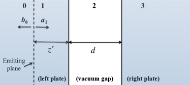
Figure 10: Two parallel plates separated by a vacuum gap of width $d$. The vertical dashed line inside the left plate indicates the position of an emitting plane that contains the radiation sources that generate the field amplitudes $\bm{b}_{0}$ and $\bm{a}_{1}$.

Let us focus now on the analysis of the power emitted by a plane inside the left plate, see Fig. 10. This emitting plane defines a fictitious interface between layers 0 and 1, which are both inside the left plate. To determine the power emitted to the right plate we first compute the field amplitudes $\bm{a}_{1}$ on the right hand side of the plane. For this purpose we make of use of Eq. (104), where in this case $l=0$ and $N=3$. Taking into account that $\hat{S}_{12}(0,0)=0$, it is straightforward to show that

$$\bm{a}_{1} = [\hat{M}_{11,1}-\hat{M}_{12,1}\hat{M}^{-1}_{22,1}\hat{M}_{21,1}]^{-1}\bm{p}_{z}+$$ (107)

$$[\hat{M}_{21,1}-\hat{M}_{22,1}\hat{M}^{-1}_{12,1}\hat{M}_{11,1}]^{-1}\bm{p}_{\parallel}$$

$$= [\hat{M}^{-1}_{1}]_{11}\bm{p}_{z}+[\hat{M}^{-1}_{1}]_{12}\bm{p}_{\parallel}.$$

To compute $Q_{1\to 3}$, it is convenient to calculate the Poynting vector in the vacuum gap. For this purpose, we need the field amplitudes in that layer. From Eq. (80), it is easy to deduce that these amplitudes are given in terms of $\bm{a}_{1}$ as follows

$$\bm{a}_{2}=\hat{D}\hat{S}_{11}(1,2)\bm{a}_{1},$$ (108)

where $\hat{D}\equiv[\hat{1}-\hat{S}_{12}(1,2)\hat{S}_{21}(2,3)]^{-1}$ and

$$\bm{b}_{2} = \left[\hat{1}-\hat{S}_{21}(2,3)\hat{S}_{12}(1,2)\right]^{-1}\hat{S}_{21}(2,3)\hat{S}_{11}(1,2)\bm{a}_{1}$$ (109)

$$= \hat{S}_{21}(2,3)\bm{a}_{2}.$$

It is worth stressing that the different elements of the scattering matrix that appear in the previous expressions can be factorized into scattering matrices $\tilde{S}$ containing only information about the interfaces of the layered system, which are basically the Fresnel coefficients of the structure, and phase factors describing the propagation between these interfaces. In particular, from Eq. (92) it is easy to show that

$$\hat{S}_{11}(1,2) = \tilde{S}_{11}(1,2)\hat{f}^{+}_{1}(z^{\prime})$$ (110)

$$\hat{S}_{12}(1,2) = \tilde{S}_{12}(1,2)e^{iq_{2}d}$$ (111)

$$\hat{S}_{21}(2,3) = \tilde{S}_{21}(2,3)e^{iq_{2}d},$$ (112)

where $q_{2}=\sqrt{\omega^{2}-k^{2}}$ is the $z$-component of the wave vector in the vacuum gap and

$$\hat{f}^{+}_{1}(z^{\prime})=\left(\begin{array}[]{cc}e^{iq_{1,1}z^{\prime}}&0\\ 0&e^{iq_{2,1}z^{\prime}}\end{array}\right).$$ (113)

Here, $q_{i,1}$ (with $i=1,2$) are the $z$-components of the two allowed wave vectors in the medium 1. On the other hand, the $\tilde{S}$-matrices can be computed directly from the interface matrices as follows [see Eq. (92)]

$$\tilde{S}_{11}(1,2) = \hat{I}^{-1}_{11}(1,2)$$ (114)

$$\tilde{S}_{12}(1,2) = -\hat{I}^{-1}_{11}(1,2)\hat{I}_{12}(1,2)$$ (115)

$$\tilde{S}_{21}(2,3) = \hat{I}_{21}(2,3)\hat{I}^{-1}_{11}(2,3).$$ (116)

In terms of the amplitudes $\bm{a}_{2}$ and $\bm{b}_{2}$, the fields in the vacuum gap at $z=0$ are given by [see Eq. (73)]

$$\left(\begin{array}[]{c}\bm{e}_{\parallel}(0)\\ \bm{h}_{\parallel}(0)\end{array}\right)_{2}=\left(\begin{array}[]{c}\hat{M}_{11,2}\left[\bm{a}_{2}-e^{iq_{2}d}\bm{b}_{2}\right]\\ \bm{a}_{2}+e^{iq_{2}d}\bm{b}_{2}\end{array}\right),$$ (117)

where we have used that $\hat{M}_{12,2}=-\hat{M}_{11,2}$, valid for any isotropic system. Thus, the $z$-component of the Poynting vector evaluated at $z=0$ in the vacuum gap reads

$$S_{z}(\omega,{\bf k},z^{\prime}) = \frac{1}{4\omega}\sqrt{\frac{\mu_{0}}{\epsilon_{0}}}\left\{\bm{h}^{\dagger}_{\parallel}(0)\bm{e}_{\parallel}(0)+\bm{e}^{\dagger}_{\parallel}(0)\bm{h}_{\parallel}(0)\right\}_{2}$$ (118)

$$= \frac{1}{4\omega}\sqrt{\frac{\mu_{0}}{\epsilon_{0}}}\left\{\bm{a}^{\dagger}_{2}\left(\hat{M}_{11,2}+\hat{M}^{\dagger}_{11,2}\right)\bm{a}_{2}-\right.$$

$$e^{i(q_{2}-q^{\ast}_{2})d}\bm{b}^{\dagger}_{2}\left(\hat{M}_{11,2}+\hat{M}^{\dagger}_{11,2}\right)\bm{b}_{2}+$$

$$e^{-iq^{\ast}_{2}d}\bm{b}^{\dagger}_{2}\left(\hat{M}_{11,2}-\hat{M}^{\dagger}_{11,2}\right)\bm{a}_{2}-$$

$$\left.e^{iq_{2}d}\bm{a}^{\dagger}_{2}\left(\hat{M}_{11,2}-\hat{M}^{\dagger}_{11,2}\right)\bm{b}_{2}\right\}.$$

Moreover, since

$$\hat{M}_{11,2}=\frac{1}{q_{2}}\left(\begin{array}[]{cc}\omega^{2}-k^{2}_{y}&k_{x}k_{y}\\ k_{x}k_{y}&\omega^{2}-k^{2}_{x}\end{array}\right)\equiv\frac{1}{q_{2}}\hat{A}$$ (119)

and $q_{2}$ is either real (for $k<\omega$) or purely imaginary (for $k>\omega$), Eq. (118) reduces to

$$S_{z}(\omega,{\bf k},z^{\prime})=\frac{1}{2q_{2}\omega}\sqrt{\frac{\mu_{0}}{\epsilon_{0}}}\times\hskip 113.81102pt$$ (120)

$$\left\{\begin{array}[]{ll}\bm{a}^{\dagger}_{2}\hat{A}\bm{a}_{2}-\bm{b}^{\dagger}_{2}\hat{A}\bm{b}_{2},&k<\omega\\ e^{-iq^{\ast}_{2}d}\bm{b}^{\dagger}_{2}\hat{A}\bm{a}_{2}-e^{iq_{2}d}\bm{a}^{\dagger}_{2}\hat{A}\bm{b}_{2},&k>\omega,\end{array}\right.$$ (123)

where the first term provides the contribution of propagating waves and the second one corresponds to the contribution of evanescent waves.

From this point on, the rest of the calculation is pure algebra and we will not describe it here in detail. Let us simply say that the basic idea is to use Eqs. (108) and (109) to express the Poynting vector in Eq. (120) in terms of the field amplitude $\bm{a}_{1}$. Then, using Eq. (107) and the fluctuation-dissipation theorem of Eq. (105) one can calculate the statistical average of the Poynting vector. Let us mention that the calculation can be greatly simplified by rotating every $2\times 2$ matrix appearing in the problem from the Cartesian basis ($x$-$y$) to the basis of $s$- and $p$-polarized waves. This can be done via the unitary matrix

$$\hat{R}\equiv\frac{1}{k}\left(\begin{array}[]{cc}k_{x}&k_{y}\\ k_{y}&-k_{x}\end{array}\right),$$ (124)

which is the matrix that defines the transformation that diagonalizes the matrix $\hat{A}$, i.e.

$$\hat{A}_{d}\equiv\hat{R}\hat{A}\hat{R}=\left(\begin{array}[]{cc}\omega^{2}&0\\ 0&q^{2}_{2}\end{array}\right).$$ (125)

Finally, after integrating over all possible values of $\omega$, ${\bf k}$, and $z^{\prime}$, see Eq. (106), one arrives at the following result for the power per unit of area transferred from the left plate to the right one

$$Q_{1\rightarrow 3}(d,T_{1})=\int^{\infty}_{0}\frac{d\omega}{2\pi}\Theta(\omega,T_{1})\int\frac{d{\bf k}}{(2\pi)^{2}}\tau(\omega,{\bf k},d),$$ (126)

where $\tau(\omega,{\bf k},d)$ is the total transmission coefficient of the electromagnetic modes and it is given by

$$\tau(\omega,{\bf k},d)=\left\{\begin{array}[]{ll}\mbox{Tr}\left\{[\hat{1}-\bar{S}_{12}(1,2)\bar{S}^{\dagger}_{12}(1,2)]\bar{D}^{\dagger}[\hat{1}-\bar{S}^{\dagger}_{21}(2,3)\bar{S}_{21}(2,3)]\bar{D}\right\},&k<\omega\;\;\mbox{(propagating waves)}\\ \mbox{Tr}\left\{[\bar{S}_{12}(1,2)-\bar{S}^{\dagger}_{12}(1,2)]\bar{D}^{\dagger}[\bar{S}^{\dagger}_{21}(2,3)-\bar{S}_{21}(2,3)]\bar{D}\right\}e^{-2|q_{2}|d},&k>\omega\;\;\mbox{(evanescent waves)}\end{array}\right..$$ (127)

Here, the $2\times 2$ matrices indicated by a bar are defined as follows

$$\bar{D} \equiv \hat{A}^{1/2}_{d}\hat{R}\hat{D}\hat{R}\hat{A}^{-1/2}_{d}$$ (128)

$$\bar{D}^{\dagger} \equiv \hat{A}^{-1/2}_{d}\hat{R}\hat{D}^{\dagger}\hat{R}\hat{A}^{1/2}_{d}.$$ (129)

Following a similar reasoning, one can compute the power per unit of area transfer from the right plate to the left one and the final result reads

$$Q_{3\rightarrow 1}(d,T_{3})=\int^{\infty}_{0}\frac{d\omega}{2\pi}\Theta(\omega,T_{3})\int\frac{d{\bf k}}{(2\pi)^{2}}\tau(\omega,{\bf k},d),$$ (130)

where $\tau(\omega,{\bf k},d)$ is also given by Eq. (127). Thus, the net power per unit of area exchanged by the plates is given by Eqs. (2) and (3) in section II. To conclude, let us stress that in the manuscript $\omega$ is meant to be an angular frequency.

Appendix C Dispersion relations

In this appendix we provide the solution of the eigenvalue problem of Eqs. (40) and (57) that give the dispersion relations of the electromagnetic modes that can exist inside the materials considered in this work. In particular, we focus here on three cases of special interest for our discussions in the main body of the manuscript.

Case 1: $\hat{\epsilon}=diag[\epsilon_{xx},\epsilon_{xx},\epsilon_{zz}]$. This situation is of relevance for the case in which the magnetic field is perpendicular to the plate surfaces, see section IIIA. In this case, the allowed $q$-values are given by

$$q^{2}_{\rm o}=\epsilon_{xx}\omega^{2}-k^{2},\;\;q^{2}_{\rm e}=\epsilon_{xx}\omega^{2}-k^{2}\epsilon_{xx}/\epsilon_{zz}.$$ (131)

Case 2: $\hat{\epsilon}=diag[\epsilon_{xx},\epsilon_{zz},\epsilon_{zz}]$. This situation is relevant for the case in which the magnetic field is parallel to the plate surfaces, see section IIIB, and the allowed $q$-values are given by

$$q^{2}_{\rm o}=\epsilon_{zz}\omega^{2}-k^{2},\;\;q^{2}_{\rm e}=\epsilon_{xx}\omega^{2}-k^{2}\epsilon_{xx}/\epsilon_{zz}.$$ (132)

Case 3: the diagonal elements of $\hat{\epsilon}$ are $\epsilon_{xx}$ and $\epsilon_{yy}=\epsilon_{zz}$, while the only non-vanishing off-diagonal elements are $\epsilon_{yz}=-\epsilon_{zy}$. This situation is relevant for the case in which the magnetic field is parallel to the plate surfaces, see section IIIB. In this case, the allowed $q$-values adopt the following form

$$q^{2}_{\rm o,1}=\epsilon_{xx}\omega^{2}-k^{2},\;\;q^{2}_{\rm o,2}=(\epsilon^{2}_{yy}+\epsilon^{2}_{yz})\omega^{2}/\epsilon_{yy}-k^{2}.$$ (133)

Appendix D Surface electromagnetic modes

We briefly describe here how we determine the dispersion relation of the surface electromagnetic modes in our system and we also provide the results for some configurations of special interest.

Let us consider a structure containing $N$ planar layers. From Eq. (91), it is easy to show that the field amplitudes in layers $l$ and $l+1$ are related as follows

$$\left(\begin{array}[]{c}\bm{a}_{l}\\ \bm{b}_{l}\end{array}\right) = \left(\begin{array}[]{cc}\hat{f}^{+}_{l}&\hat{0}\\ \hat{0}&\hat{1}\end{array}\right)^{-1}\hat{I}(l,l+1)\left(\begin{array}[]{cc}\hat{1}&\hat{0}\\ \hat{0}&\hat{f}^{-}_{l+1}\end{array}\right)\left(\begin{array}[]{c}\bm{a}_{l+1}\\ \bm{b}_{l+1}\end{array}\right)$$ (142)

$$\equiv \hat{I}^{\prime}(l,l+1)\left(\begin{array}[]{c}\bm{a}_{l+1}\\ \bm{b}_{l+1}\end{array}\right).$$ (145)

Now, using this relation recursively we can relate the field amplitudes in the first and last layers as follows

$$\left(\begin{array}[]{c}\bm{a}_{1}\\ \bm{b}_{1}\end{array}\right)=\left[\prod^{N-1}_{l=1}\hat{I}^{\prime}(l,l+1)\right]\left(\begin{array}[]{c}\bm{a}_{N}\\ \bm{b}_{N}\end{array}\right)\equiv\hat{I}^{S}\left(\begin{array}[]{c}\bm{a}_{N}\\ \bm{b}_{N}\end{array}\right).$$ (146)

The condition for an eigenmode of the system is that $\bm{a}_{1}=\bm{b}_{N}={\bf 0}$, which from the previous equation implies that $\hat{I}^{S}_{11}\bm{a}_{N}={\bf 0}$. The condition for having a non-trivial solution of this equation is that $\det\hat{I}^{S}_{11}=0$, which is the condition that surface electromagnetic modes must satisfy. In our plate-plate geometry, the $4\times 4$ matrix $\hat{I}^{S}$ is simply given by

$$\hat{I}^{S}=\hat{I}(1,2)\left(\begin{array}[]{cc}e^{-iq_{2}d}\hat{1}&\hat{0}\\ \hat{0}&e^{iq_{2}d}\hat{1}\end{array}\right)\hat{I}(2,3),$$ (147)

where let us recall that $q_{2}=\sqrt{\omega^{2}-k^{2}}$. Thus, the condition for an eigenmode of the system reads

$$\det[\hat{I}_{11}(1,2)\hat{I}_{11}(2,3)e^{-iq_{2}d}+\hat{I}_{12}(1,2)\hat{I}_{21}(2,3)e^{iq_{2}d}]=0.$$ (148)

In what follows, we provide the explicit equations satisfied by the dispersion relation of the surface waves in the three cases considered in Appendix C.

Case 1: In this case, Eq. (148) leads to

$$e^{-iq_{2}d}=\pm\left(\frac{q_{\rm e}-\epsilon_{xx}q_{2}}{q_{\rm e}+\epsilon_{xx}q_{2}}\right),$$ (149)

where $q_{\rm e}$ is given in Eq. (131). This equations reduces to Eq. (18) in the electrostatic limit $k\gg\omega/c$.

Case 2: Here, assuming that the surface wave propagates along the $x$-direction, its dispersion relation satisfies the following relation

$$e^{-iq_{2}d}=\pm\left(\frac{q_{\rm e}-\epsilon_{xx}q_{2}}{q_{\rm e}+\epsilon_{xx}q_{2}}\right),$$ (150)

where $q_{\rm e}$ is given in Eq. (132). In the electrostatic limit, this equation reduces to Eq. (18).

Case 3: In this case, and assuming that the surface waves propagate along the $y$-direction, its dispersion relation is given by the solution of the following equation

$$e^{-2iq_{2}d}=\frac{(\eta_{yy}q_{\rm o,2}-q_{2}+\eta_{yz}k)(\eta_{yy}q_{\rm o,2}-q_{2}-\eta_{yz}k)}{(\eta_{yy}q_{\rm o,2}+q_{2}+\eta_{yz}k)(\eta_{yy}q_{\rm o,2}+q_{2}-\eta_{yz}k)},$$ (151)

where $\eta_{yy}=\epsilon_{yy}/(\epsilon_{yy}^{2}+\epsilon_{yz}^{2})$, $\eta_{yz}=-\epsilon_{yz}/(\epsilon_{yy}^{2}+\epsilon_{yz}^{2})$, and $q_{\rm o,2}$ is given in Eq. (133). In the electrostatic limit this equation reduces to Eq. (23).

References

- (1) R. Siegel and J. R. Howell, Thermal Radiation Heat Transfer, 4th ed. (Taylor and Francis, New York, 2002).
- (2) Z. M. Zhang, Nano/microscale Heat Transfer, (McGraw-Hill, New York, NY, 2007).
- (3) K. Joulain, J. P. Mulet, F. Marquier, R. Carminati, and J. J. Greffet, Surface Electromagnetic Waves Thermally Excited: Radiative Heat Transfer, Coherence Properties and Casimir Forces Revisited in the Near Field, Surf. Sci. Rep. 57, 59 (2005).
- (4) A. I. Volokitin and B. N. J. Persson, Near-Field Radiative Heat Transfer and Noncontact Friction, Rev. Mod. Phys. 79, 1291 (2007).
- (5) S. Basu, Z. M. Zhang, and C. J. Fu, Review of Near-Field Thermal Radiation and its Application to Energy Conversion, Int. J. Energy Res. 33, 1203 (2009).
- (6) B. Song, A. Fiorino, E. Meyhofer, and P. Reddy, Near-Field Radiative Thermal Transport: From Theory to Experiment, AIP Advances 5, 053503 (2015).
- (7) D. Polder and M. Van Hove, Theory of Radiative Heat Transfer between Closely Spaced Bodies, Phys. Rev. B 4, 3303 (1971).
- (8) S. M. Rytov, Theory of Electric Fluctuations and Thermal Radiation, (Air Force Cambridge Research Center, Bedford, MA, 1953).
- (9) S. M. Rytov, Y. A. Kravtsov, and V. I. Tatarskii, Principles of Statistical Radiophysics, Vol. 3 (Springer-Verlag, Berlin Heidelberg, 1989).
- (10) C. M. Hargreaves, Anomalous Radiative Transfer between Closely-Spaced Bodies, Phys. Lett. A 30, 491 (1969).
- (11) G. A. Domoto, R. F. Boehm, and C. L. Tien, Experimental Investigation of Radiative Transfer between Metallic Surfaces at Cryogenic Temperatures, J. Heat Transfer 92, 412 (1970).
- (12) A. Kittel, W. Müller-Hirsch, J. Parisi, S.-A. Biehs, D. Reddig, and M. Holthaus, Near-field Heat Transfer in a Scanning Thermal Microscope, Phys. Rev. Lett. 95, 224301 (2005).
- (13) A. Narayanaswamy, S. Shen, and G. Chen, Near-Field Radiative Heat Transfer between a Sphere and a Substrate, Phys. Rev. B 78, 115303 (2008).
- (14) L. Hu, A. Narayanaswamy, X. Y. Chen, and G. Chen, Near-Field Thermal Radiation between Two Closely Spaced Glass Plates Exceeding Planck’s Blackbody Radiation Law, Appl. Phys. Lett. 92, 133106 (2008).
- (15) E. Rousseau, A. Siria, G. Jourdan, S. Volz, F. Comin, J. Chevrier, and J.-J, Greffet, Radiative Heat Transfer at the Nanoscale, Nat. Photonics 3, 514 (2009).
- (16) S. Shen, A. Narayanaswamy, and G. Chen, Surface Phonon Polaritons Mediated Energy Transfer between Nanoscale Gaps, Nano Lett. 9, 2909 (2009).
- (17) R. S. Ottens, V. Quetschke, S. Wise, A. A. Alemi, R. Lundock, G. Mueller, D. H. Reitze, D. B. Tanner, and B. F. Whiting, Near-Field Radiative Heat Transfer between Macroscopic Planar Surfaces, Phys. Rev. Lett. 107, 014301 (2011).
- (18) S. Shen, A. Mavrokefalos, P. Sambegoro, and G. Chen, Nanoscale Thermal Radiation between Two Gold Surfaces, Appl. Phys. Lett. 100, 233114 (2012).
- (19) T. Kralik, P. Hanzelka, M. Zobac, V. Musilova, T. Fort, and M. Horak, Strong Near-Field Enhancement of Radiative Heat Transfer between Metallic Surfaces, Phys. Rev. Lett. 109, 224302 (2012).
- (20) P. J. van Zwol, L. Ranno, and J. Chevrier, Tuning Near Field Radiative Heat Flux through Surface Excitations with a Metal Insulator Transition, Phys. Rev. Lett. 108, 234301 (2012).
- (21) P. J. van Zwol, S. Thiele, C. Berger, W. A. de Heer, and J. Chevrier, Nanoscale Radiative Heat Flow due to Surface Plasmons in Graphene and Doped Silicon, Phys. Rev. Lett. 109, 264301 (2012).
- (22) B. Guha, C. Otey, C. B. Poitras, S. H. Fan, and M. Lipson, Near-Field Radiative Cooling of Nanostructures, Nano Lett. 12, 4546 (2012).
- (23) J. Shi, P. Li, B. Liu, and S. Shen, Tuning Near Field Radiation by Doped Silicon, Appl. Phys. Lett. 102, 183114 (2013).
- (24) L. Worbes, D. Hellmann, and A. Kittel, Enhanced Near-Field Heat Flow of a Monolayer Dielectric Island, Phys. Rev. Lett. 110, 134302 (2013).
- (25) R. St-Gelais, B. Guha, L. X. Zhu, S. H. Fan, and M. Lipson, Demonstration of Strong Near-Field Radiative Heat Transfer between Integrated Nanostructures, Nano Lett. 14, 6971 (2014).
- (26) B. Song, Y. Ganjeh, S. Sadat, D. Thompson, A. Fiorino, V. Fernández-Hurtado, J. Feist, F. J. Garcia-Vidal, J. C. Cuevas, P. Reddy, and E. Meyhofer, Enhancement of Near-Field Radiative Heat Transfer Using Polar Dielectric Thin Films, Nat. Nanotechnol. 10, 253 (2015).
- (27) M. Lim, S. S. Lee, and B. J. Lee, Near-Field Thermal Radiation between Doped Silicon Plates at Nanoscale Gaps, Phys. Rev. B 91, 195136 (2015).
- (28) W. A. Challener, C. B. Peng, A. V. Itagi, D. Karns, W. Peng, Y. Y. Peng, X. M. Yang, X. B. Zhu, N. J. Gokemeijer, Y. T. Hsia, G. Ju, R. E. Rottmayer, M. A. Seigler, and E. C. Gage, Heat-assisted Magnetic Recording by a Near-field Transducer with Efficient Optical Energy Transfer, Nat. Photonics 3, 220 (2009).
- (29) B. C. Stipe, T. C. Strand, C. C. Poon, H. Balamane, T. D. Boone, J. A. Katine, J. L. Li, V. Rawat, H. Nemoto, A. Hirotsune, O. Hellwig, R. Ruiz, E. Dobisz, D. S. Kercher, N. Robertson, T. R. Albrecht, and B. D. Terris, Magnetic Recording at 1.5 Pb m−2 Using an Integrated Plasmonic Antenna, Nat. Photonics 4, 484 (2010).
- (30) J. B. Pendry, Radiative Exchange of Heat between Nanostructures, J. Phys. Condens. Matter 11, 6621 (1999).
- (31) Y. D. Wilde, F. Formanek, R. Carminati, B. Gralak, P. A. Lemoine, K. Joulain, J. P. Mulet, Y. Chen, J. J. Greffet, Thermal Radiation Scanning Tunnelling Microscopy, Nature (London) 444, 740 (2006).
- (32) A. Kittel, U. F. Wischnath, J. Welker, O. Huth, F. Ruting, and S. A. Biehs, Near-Field Thermal Imaging of Nanostructured Surfaces, Appl. Phys. Lett. 93, 193109 (2008).
- (33) A. C. Jones, B. T. O’Callahan, H. U. Yang, and M. B. Raschke, The Thermal Near-Rield: Coherence, Spectroscopy, Heat-Transfer, and Optical Forces, Prog. Surf. Sci. 88, 349 (2013).
- (34) R. Carminati and J. J. Greffet, Near-Field Effects in Spatial Coherence of Thermal Sources, Phys. Rev. Lett. 82, 1660 (1999).
- (35) J. J. Greffet, R. Carminati, K. Joulain, J. P. Mulet, S. P. Mainguy, and Y. Chen, Coherent Emission of Light by Thermal Sources, Nature (London) 416, 61 (2002).
- (36) C. Otey, W. T. Lau, and S. Fan, Thermal Rectification through Vacuum, Phys. Rev. Lett. 104, 154301 (2010).
- (37) A. W. Rodriguez, O. Ilic, P. Bermel, I. Celanovic, J. D. Joannopoulos, M. Soljacic, and S. G. Johnson, Frequency-Selective Near-Field Radiative Heat Transfer between Photonic Crystal Slabs: A Computational Approach for Arbitrary Geometries and Materials, Phys. Rev. Lett. 107, 114302 (2011).
- (38) P. Ben-Abdallah and S. A. Biehs, Near-Field Thermal Transistor, Phys. Rev. Lett. 112, 044301 (2014).
- (39) R. Messina and P. Ben-Abdallah, Graphene-Based Photovoltaic Cells for Near-Field Thermal Energy Conversion, Sci. Rep. 3, 1383 (2013).
- (40) A. Lenert, D. M. Bierman, Y. Nam, W. R. Chan, I. Celanovic, M. Soljacic, and E. N. Wang, A Nanophotonic Solar Thermophotovoltaic Device, Nat. Nanotechnol. 9, 126 (2014).
- (41) J. W. Schwede, I. Bargatin, D. C. Riley, B. E. Hardin, S. J. Rosenthal, Y. Sun, F. Schmitt, P. Pianetta, R. T. Howe, Z. X. Shen, and N. A. Melosh, Photon-Enhanced Thermionic Emission for Solar Concentrator Systems, Nat. Mater. 9, 762 (2010).
- (42) J. P. Mulet, K. Joulain, R. Carminati, and J. J. Greffet, Enhanced Radiative Heat Transfer at Nanometric Distances, Microscale Therm. Eng. 6, 209 (2002).
- (43) C. J. Fu and Z. M. Zhang, Nanoscale Radiation Heat Transfer for Silicon at Different Doping Levels, Int. J. Heat Mass Transfer 49, 1703 (2006).
- (44) E. Rousseau, M. Laroche, and J. J. Greffet, Radiative Heat Transfer at Nanoscale Mediated by Surface Plasmons for Highly Doped Silicon, Appl. Phys. Lett. 95, 231913 (2009).
- (45) I. S. Nefedov and C. R. Simovski, Giant Radiation Heat Transfer Through Micron Gaps, Phys. Rev. B 84, 195459 (2011).
- (46) S. A. Biehs, M. Tschikin, and P. Ben-Abdallah, Hyperbolic Metamaterials as an Analog of a Blackbody in the Near Field, Phys. Rev. Lett. 109, 104301 (2012).
- (47) Y. Guo, C. L. Cortes, S. Molesky, and Z. Jacob, Broadband super-Planckian Thermal Emission from Hyperbolic Metamaterials, Appl. Phys. Lett. 101, 131106 (2012).
- (48) D. R. Smith and D. Schurig, Electromagnetic Wave Propagation in Media with Indefinite Permittivity and Permeability Tensors, Phys. Rev. Lett. 90, 077405 (2003).
- (49) A. Poddubny, I. Iorsh, P. Belov, and Y. Kivshar, Hyperbolic Metamaterials, Nat. Photonics 7, 958 (2013).
- (50) P. Shekhar, J. Atkinson, and Z. Jacob, Hyperbolic Metamaterials: Fundamentals and Applications, Nano Convergence 1, 14 (2014).
- (51) S. A. Biehs, M. Tschikin, R. Messina, and P. Ben-Abdallah, Super-Planckian Near-Field Thermal Emission with Phonon-Polaritonic Hyperbolic Metamaterials, Appl. Phys. Lett. 102, 131106 (2013).
- (52) M. Tschikin, S. A. Biehs, R. Messina, P. Ben-Abdallah, On the Limits of the Effective Description of Hyperbolic Materials in Presence of Surface Waves, J. Opt. 15, 105101 (2013).
- (53) Y. Guo and Z. B. Jacob, Thermal Hyperbolic Metamaterials, Opt. Express 21, 15014 (2013).
- (54) C. Simovski, S. Maslovski, I. Nefedov, and S. Tretyakov, Optimization of Radiative Heat Transfer in Hyperbolic Metamaterials for Thermophotovoltaic Applications, Opt. Express 21, 14988 (2013).
- (55) X. L. Liu, R. Z. Zhang, and Z. M. Zhang, Near-Field Thermal Radiation between Hyperbolic Metamaterials: Graphite and Carbon Nanotubes, Appl. Phys. Lett. 103, 213102 (2013).
- (56) X. L. Liu, R. Z. Zhang, and Z. M. Zhang, Near-Field Radiative Heat Transfer with Doped-Silicon Nanostructured Metamaterials, Int. J. Heat Mass Transfer 73, 389 (2014).
- (57) Y. Guo and Z. Jacob, Fluctuational Electrodynamics of Hyperbolic Metamaterials, J. Appl. Phys. 115, 234306 (2014).
- (58) O. D. Miller, S. G. Johnson, and A. W. Rodriguez, Effectiveness of Thin Films in Lieu of Hyperbolic Metamaterials in the Near Field, Phys. Rev. Lett. 112, 157402 (2014).
- (59) S. Lang, M. Tschikin, S. A. Biehs, A. Yu. Petrov, and M. Eich, Large Penetration Depth of Near-Field Heat Flux in Hyperbolic Media, Appl. Phys. Lett. 104, 121903 (2014).
- (60) I. S. Nefedov and L. A. Melnikov, Super-Planckian Far-Zone Thermal Emission from Asymmetric Hyperbolic Metamaterials, Appl. Phys. Lett. 105, 161902 (2014).
- (61) M. Tschikin, S. A. Biehs, P. Ben-Abdallah, S. Lang, A. Yu. Petrov, and M. Eich, Radiative Heat Flux Predictions in Hyperbolic Metamaterials, J. Quant. Spectrosc. Radiat. Transf. 158, 17 (2015).
- (62) P. J. van Zwol, K. Joulain, P. Ben-Abdallah, and J. Chevrier, Phonon Polaritons Enhance Near-Field Thermal Transfer Across the Phase Transition of VO2, Phys. Rev. B 84, 161413(R) (2011).
- (63) P. J. van Zwol, K. Joulain, P. Ben-Abdallah, J. J. Greffet, and J. Chevrier, Fast Nanoscale Heat-Flux Modulation with Phase-Change Materials, Phys. Rev. B 83, 201404(R) (2011).
- (64) L. J. Cui, Y. Huang, and J. Wang, Near-Field Radiative Heat Transfer between Chiral Metamaterials, J. Appl. Phys. 112, 084309 (2012).
- (65) Y. Huang, S. V. Boriskina, and G. Chen, Electrically Tunable Near-Field Radiative Heat Transfer via Ferroelectric Materials, Appl. Phys. Lett. 105, 244102 (2014).
- (66) K. Chen, P. Santhanam, S. Sandhu, L. Zhu, and S. Fan, Heat-Flux Control and Solid-State Cooling by Regulating Chemical Potential of Photons in Near-Field Electromagnetic Heat Transfer, Phys. Rev. B 91, 134301 (2015).
- (67) A. Zvezdin and V. Kotov, Modern Magnetooptics and Magnetooptical Materials (IOP, Bristol, 1997).
- (68) S. A. Biehs, P. Ben-Abdallah, F. S. S. Rosa, K. Joulain, and J.-J. Greffet, Nanoscale Heat Flux between Nanoporous Materials, Opt. Express 19, A1088 (2011).
- (69) M. S. Kushwaha, Plasmons and Magnetoplasmons in Semiconductor Heterostructures, Surf. Sci. Rep. 41, 1 (2001).
- (70) R. F. Wallis, in A.D. Boardman (Ed.), Electromagnetic Surface Modes, (Wiley, New York, 1982), p. 575.
- (71) E. D. Palik, B. Kaplan, B. W. Gammon, H. Kaplan, J. J. Quinn, and B. F. Wallis, Surface Magnetoplasmon-Optic Phonon Modes in InSb, Phys. Lett. A 45, 143 (1973).
- (72) A. Hartstein, E. Burstein, E. D. Palik, R. W. Gammon, and B. W. Henvis, Investigation of Optic-Phonon-Magnetoplasmon-Type Surface Polaritons on n-Insb, Phys. Rev. B 12, 3186 (1975).
- (73) E. D. Palik, R. Kaplan, R. W. Gammon, H. Kaplan, R. F. Wallis, and J. J. Quinn, Coupled Surface Magnetoplasmon-Optic-Phonon Polariton Modes on InSb, Phys. Rev. B 13, 2497 (1976).
- (74) L. Remer, E. Mohler, W. Grill, and B. Lüthi, Nonreciprocity in the Optical Reflection of Magnetoplasmas, Phys. Rev. B 30, 3277 (1984).
- (75) P. O. Chapuis, S. Volz, C. Henkel, K. Joulain, and J. J. Greffet, Effects of Spatial Dispersion in Near-Field Radiative Heat Transfer between Two Parallel Metallic Surfaces, Phys. Rev. B 77, 035431 (2008).
- (76) B. Caballero, A. García-Martín, and J. C. Cuevas, Generalized Scattering-Matrix Approach for Magneto-Optics in Periodically Patterned Multilayer Systems, Phys. Rev. B 85, 245103 (2012).
- (77) D. M. Whittaker and I. S. Culshaw, Scattering-Matrix Treatment of Patterned Multilayer Photonic Structures, Phys. Rev. B 60, 2610 (1999).
- (78) L. Landau, E. Lifshitz, and L. Pitaevskii, Course of Theoretical Physics, (Pergamon, New York, 1980), Vol. 9, Part 2.
- (79) Yu. A. Il’inskii and L. V. Keldysh, Electromagnetic Response of Material Media, (Plenum Press, New York, 1994).