Thermoelectricity of interacting particles: A numerical approach

Abstract

A method for computing the thermopower in interacting systems is proposed. This approach, which relies on Monte Carlo simulations, is illustrated first for a diatomic chain of hard-point elastically colliding particles and then in the case of a one-dimensional gas with (screened) Coulomb interparticle interaction. Numerical simulations up to $N>10^{4}$ particles confirm the general theoretical arguments for momentum-conserving systems and show that the thermoelectric figure of merit increases linearly with the system size.

I Introduction

Thermoelectric materials are of interest due to their ability to convert waste heat into electricity by the Seebeck effect or use electricity for cooling by the Peltier effect dresselhaus ; snyder ; shakuori ; dubi ; thermo_review . The efficiency of a thermoelectric material is a monotonously growing function of the dimensionless figure of merit,

$$ZT=\frac{\sigma S^{2}}{\kappa}\,T,$$ (1)

where $T$ is the temperature, $\sigma$ is the electrical conductivity, $\kappa$ is the thermal conductivity, and $S$ is the thermopower (or Seebeck coefficient). Increasing $ZT$ is a challenging task due to the interdependency of transport coefficients. In particular, the electrical conductivity and the electronic contribution to the thermal conductivity are related by the Wiedemann-Franz law kittel , which, follows at low enough temperatures from the single-particle Fermi liquid theory, states that the ratio $\sigma T/\kappa$ is constant. Such limitations could be overcome, in principle, by the energy filtering mechanism mahansofo ; linke1 ; linke2 , i.e., when transmission of electrons is possible only within a tiny energy window.

On the other hand, very little is known about the thermoelectric properties of interacting systems. In this case, analytical results are rare and numerical simulations face difficult problems. To numerically evaluate $ZT$, one may put the system into contact with two thermochemical baths (reservoirs) allowing for particle exchange with the system. The reservoirs are tuned at different temperatures and electrochemical potentials in order to maintain stationary particle and heat currents. By analyzing the response of these currents to the temperature and electrochemical potential difference, one can evaluate the transport coefficients and, in turn, $ZT$, with Eq. (1). This method has been successfully applied to the one-dimensional (1D) dimerized gas of interacting hard-point particles Benenti . In that model, due to the fact that particles only interact via instantaneous collisions, the particles in the reservoirs are in effect decoupled from those of the system. As such the reservoirs can be modeled as ideal gases so that the simulations can be facilitated greatly (see Ref. YT for the detailed description of the algorithm). However, in more general systems with realistic interaction, the coupling between the reservoirs and the system is essential; the mere injection of particles from an ideal gas into the system may induce huge, unphysical interaction energy when an injected particle is too close to a system particle.

Given this difficulty, which is unsolved yet to the best of our knowledge, we turn to the closed heat baths Lepri03 ; Dharrev that only exchange heat with the system. We sandwich the system with two closed heat baths at different temperatures to establish a nonequilibrium setup. For interacting systems, the heat conductivity can be computed directly with this setup, but computing thermopower is challenging. In this paper, we solve this problem by the following steps: We first use the grand-canonical Monte Carlo method DFrenkel to compute the electrochemical potential, $\mu$, as a function of the particle density, $\rho$, at a given temperature; then, with our nonequilibrium setup and by molecular dynamics, we compute the density difference $\Delta\rho$ across the system, set in response to the temperature difference $\Delta T$ applied to the system. Finally, based on the established relation between $\mu$ and $\rho$, we map the density difference into the thermoelectric voltage difference, $\Delta V$, so that the thermopower is computed as $S=-\Delta V/\Delta T$. As to the electrical conductivity $\sigma$, due to the fact that closed heat baths do not support a charge current, it cannot be computed numerically with our nonequilibrium setup; However, it can be computed in equilibrium simulations by using the Green-Kubo formula kubo .

To test and illustrate the method for computing the thermopower in nonequlibrium simulations, we first consider the 1D dimerized hard-point gas model Casati86 . Then, we numerically investigate the case of a 1D gas of particles with nearest-neighbor Coulomb interaction, modeling a screened Coulomb interaction between electrons. Due to momentum conservation (more generally, due to the existence of a single relevant conserved quantity), we expect on general grounds Benenti that the figure of merit $ZT$ diverges in the thermodynamic limit, implying that the Carnot efficiency is reached in this limit. This result, so far illustrated by means of toy models Benenti ; Benenti14 , is here confirmed in a more realistic model. Moreover, $ZT$ exhibits a rapid, linear growth with the system size, which is a consequence of the recently reported Fourier-like behavior of thermal conductivity Zhong12 ; chen ; dhar ; wang ; savin ; Fourierlike .

II Numerical method

The equations connecting fluxes and thermodynamic forces within linear irreversible thermodynamics are callen ; degrootmazur

$$\left(\begin{array}[]{c}j_{\rho}\\ j_{u}\end{array}\right)=\left(\begin{array}[]{cc}L_{\rho\rho}&L_{\rho u}\\ L_{u\rho}&L_{uu}\end{array}\right)\left(\begin{array}[]{c}-\nabla(\beta\mu)\\ \nabla\beta\end{array}\right),$$ (2)

where $j_{\rho}$ is the local particle current, $j_{u}$ is the local energy current, $\mu$ is the electrochemical potential, and $\beta=1/(k_{B}T)$ is the inverse temperature (we set the Boltzmann constant $k_{B}=1$). The kinetic coefficients $L_{ij}$ (with $i,j=\rho,u$) are related to the familiar transport coefficients as

$$\sigma=\frac{e^{2}}{T}\,L_{\rho\rho},\quad\kappa=\frac{1}{T^{2}}\frac{\det\mathbb{L}}{L_{\rho\rho}},\quad S=\frac{1}{eT}\left(\frac{L_{\rho u}}{L_{\rho\rho}}-\mu\right);$$ (3)

here $e$ is the charge of each particle (set to be $e=1$), and $\det\mathbb{L}$ denotes the determinant of the (Onsager) matrix of kinetic coefficients. Thermodynamics imposes $\det\mathbb{L}\geq 0$, $L_{\rho\rho}\geq 0$, and $L_{uu}\geq 0$, and the Onsager reciprocity relations ensure that $L_{u\rho}=L_{\rho u}$. Following Eq. (1), the thermoelectric figure of merit thus reads

$$ZT=\frac{(L_{u\rho}-\mu L_{\rho\rho})^{2}}{\det\mathbb{L}}.$$ (4)

Hereafter we describe a method for the computation of the transport coefficients, and consequently $ZT$, in a generic interacting system. Note that, even though we consider the particle and energy flows along one direction, the motion inside the system could be, in principle, two- or three-dimensional.

Thermal conductivity.– We compute the thermal conductivity by nonequilibrium simulations. Two heat baths Lepri03 ; Dharrev at temperatures $T_{L}=T+\Delta T/2$ and $T_{R}=T-\Delta T/2$, respectively, are connected to the two ends of the system. Then the system is evolved and after a long enough relaxation stage, when the stationary state has been established, the heat conductivity is evaluated as $\kappa=\overline{j_{u}}/(\Delta T/L)$, where the overbar denotes time averaging and $L$ is the system size along the direction of the heat flow. The distributions of the temperature and the particle density are calculated at the stationary state as well. The temperature is numerically computed as $T(x)=2\epsilon_{k}(x)/\rho(x)$, where $\rho(x)=\overline{\sum_{i}\delta(x-x_{i})}$ is the particle density and $\epsilon_{k}(x)=\overline{\sum_{i}\frac{m_{i}v_{i}^{2}}{2}\delta(x-x_{i})}$ is the kinetic energy density Dhar01 .

Thermopower.– We use the nonequilibrium setup with heat baths described above and prepare the system in the stationary state. The thermopower is defined as the magnitude of the induced thermoelectric voltage in response to the temperature difference across the system, i.e., $S\equiv-\Delta\mu/e\Delta T$, where $\Delta\mu=\mu_{L}-\mu_{R}=e\Delta V$ is the induced electrochemical potential difference. In our simulations, we first compute the particle density $\rho_{L}$ and $\rho_{R}$ at the two ends of the system, and then map these values into $\mu_{L}$ and $\mu_{R}$, respectively, by means of the grand-canonical Monte Carlo method (see the Appendix A).

Electrical conductivity.– As we consider closed heat baths that do not exchange particles with the system, we cannot compute the electrical conductivity with our nonequilibrium setup. For this purpose, one can turn to equilibrium simulations by taking advantage of the Green-Kubo formula kubo .

III Numerical tests with the 1D dimerized gas model

In order to test and elucidate the grand-canonical Monte Carlo method in computing the thermopower, we first consider a gas of $N$ colliding hard-point particles with alternate masses $m$ and $M$, a paradigmatic model proposed in Ref. Casati86 and extensively investigated in the literatures Dhar01 ; Savin02 ; Grassberger02 ; Casati03 ; Politi05 ; Dharrev ; Hanggi11 ; Chen13 ; SciChina ; Chen14 ; Spohn14 ; Fourierlike ; Benenti for understanding low-dimensional transport problem. We start with the case of equal masses, $m=M$, for which the relation between the electrochemical potential and the density is the same as for the one-dimensional ideal gas in the semiclassical limit huang :

$$\mu=k_{B}T\ln(\rho\lambda).$$ (5)

Here, $\lambda=h/\sqrt{2\pi mk_{B}T}$ is the de Broglie thermal wavelength ($h$ is the Planck’s constant). The excellent agreement between this analytical expression and the numerical Monte Carlo simulations is shown in Fig. 1. It is interesting to remark that from classical thermodynamics of a one-dimensional ideal gas we obtain ${\mu}={k_{B}T}\ln({C\rho}/{\sqrt{T}})$, where the constant $C$ cannot be determined by purely classical means. On the other hand, such ambiguity is not present in the grand-canonical Monte Carlo simulations. Indeed, this method is in some sense semi-classical, in that it uses as information the value of the de Broglie thermal wavelength and the grand canonical partition function where the particles are considered as indistinguishable (see the Appendix A; the factor $1/{N!}$ in Eq. (14) is of purely quantum origin). In our units, $\lambda=1/\sqrt{T}$, and therefore $C=1$.

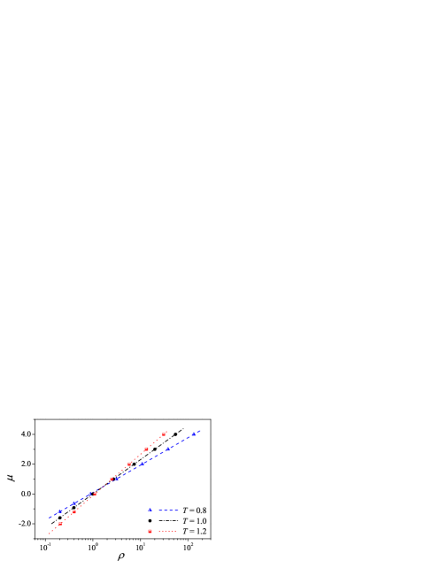
Figure 1: (Color online) Electrochemical potential versus particle density for the equal-mass ($m=M$) hard-point gas. Numerical results of the grand-canonical Monte Carlo (MC) simulations (symbols) are compared with the analytical results (lines) given by Eq. (5). Here and in the following figures we use units such that $m=1$, the Boltzmann constant $k_{B}=1$, and the de Broglie thermal wavelength $\lambda=1/\sqrt{T}$.

Size	$T^{\prime}_{L}$	$\rho_{L}$	$\mu_{L}$	$T^{\prime}_{R}$	$\rho_{R}$	$\mu_{R}$
21	1.033	0.978	-0.040	0.979	1.022	0.032
41	1.037	0.971	-0.049	0.967	1.031	0.046
81	1.041	0.965	-0.058	0.960	1.037	0.054
161	1.045	0.960	-0.066	0.956	1.042	0.061
321	1.047	0.957	-0.070	0.953	1.046	0.066
641	1.049	0.955	-0.073	0.952	1.048	0.068
1281	1.049	0.954	-0.074	0.951	1.050	0.070
2561	1.050	0.953	-0.076	0.951	1.050	0.070
5121	1.050	0.953	-0.076	0.950	1.051	0.072
10241	1.050	0.953	-0.076	0.950	1.051	0.072

Table 1: The numerically computed data for hard-point gas model. The temperatures of the two heat baths are set to be $T_{L}=1.05$ and $T_{R}=0.95$.

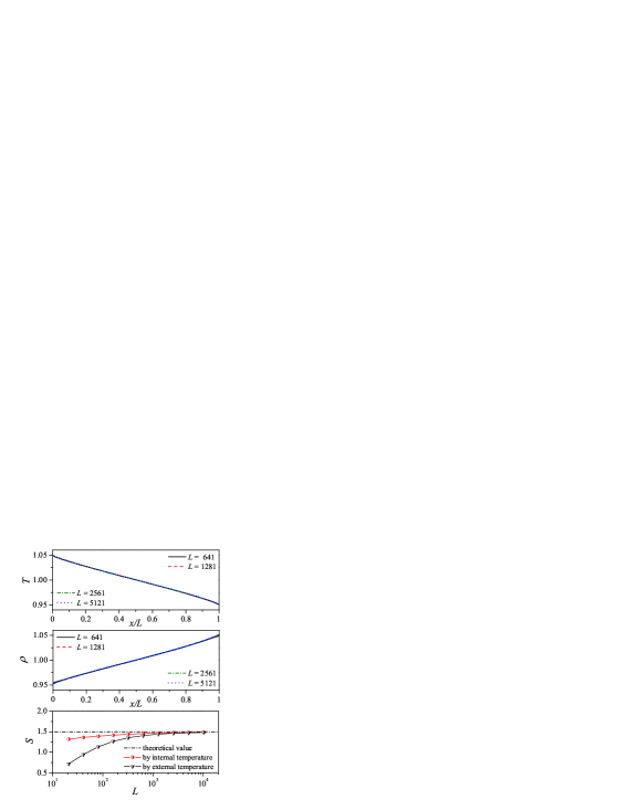
Figure 2: (Color online) The temperature profile (top panel), the density profile (middle panel), and the thermopower (bottom panel) for the hard-point gas with unequal masses $m=1$ and $M=(\sqrt{5}+1)/2$. The temperatures of the two heat baths are set to be $T_{L}=1.05$ and $T_{R}=0.95$. The dash-dotted line in the bottom panel shows the analytical result of $S=3/2$.

As shown in Fig. 1, with the grand-canonical Monte Carlo method we can numerically determine the dependence of the electrochemical potential on the particle density at a given temperature $T$. Further, we can compute the thermopower by nonequilibrium molecular simulations using two statistical thermal baths, with different temperatures $T_{L}$ and $T_{R}$, coupled to the left and the right end of the system. When the first (last) particle collides with the left (right) side of the system, it is injected back with a new speed $|v|$ determined by the distribution heatbath

$$P_{L,R}(v)=\frac{|v|m_{1,N}}{k_{B}T_{L,R}}\exp\left(-\frac{v^{2}m_{1,N}}{2k_{B}T_{L,R}}\right),$$ (6)

where $m_{1}$ and $m_{N}$ are the masses of the first and the last particle.

As an example, here we consider the gas of colliding hard-point particles with alternate masses $m=1$ and $M=(\sqrt{5}+1)/2\approx 1.618$ Fourierlike . The mean distance between two nearest-neighboring particles is set to be unity, so that the system length (size) $L$ equals the particle number $N$. Figure 2 shows the stationary temperature and density profiles (top and middle panels). The densities $\rho_{L}$ and $\rho_{R}$ at the left and right ends of the chain can be computed directly. Then the relation between $\rho$ and $\mu$ provided by the grand-canonical Monte Carlo simulations allows us to obtain the corresponding values of $\mu_{L}$ and $\mu_{R}$ and to compute the thermopower (bottom panel of Fig. 2) as $S=-\Delta\mu/e\Delta T$. It should be noted that, as shown in Table 1, for small system sizes, the internal temperatures $T^{\prime}_{L}$ and $T^{\prime}_{R}$ at the left and right ends of the system, at which the particle densities $\rho_{L}$ and $\rho_{R}$ are computed, are slightly different from the external temperatures $T_{L}$ and $T_{R}$. This discontinuity is the result of a boundary resistance, generally denoted as Kapitza resistance; see for instance Ref. Lepri03 . This boundary effect vanishes when increasing the system size; see Table 1. However, it may be relevant for small systems sizes, as shown in the bottom panel of Fig. 2, where we compare the thermopower computed by using the internal temperatures as $S=-(\mu_{L}-\mu_{R})/e(T^{\prime}_{L}-T^{\prime}_{R})$ or the external temperatures as $S=-(\mu_{L}-\mu_{R})/e(T_{L}-T_{R})$. Since we are here interested in the intrinsic transport properties of the system rather than in the details of the coupling to the heat baths, in what follows we will show results for the first method only. Moreover, we note that the first method shows a faster convergence to the asymptotic analytical value $S=3/2$ Benenti than the second one. Finally, the convergence of our numerical results for a nonintegrable model to the analytical value corroborates the validity of our computational scheme.

IV Thermoelectricity of the Coulomb gas

With the help of the above described method, now we study a 1D system of more general interaction.

IV.1 The model

The model system we consider consists of $N$ charged particles with nearest-neighbor Coulomb interaction, which is described by the Hamiltonian

$$H=\sum_{i}\left[\frac{p_{i}^{2}}{2m_{i}}+U(x_{i}-x_{i-1})\right],$$ (7)

where $m_{i}$, $x_{i}$, and $p_{i}=m_{i}\dot{x}_{i}$ are the mass, the coordinate, and the momentum of the $i$th particle, respectively, and the nearest-neighbor interaction given by $U(x)=a/x$ can be considered as a simplified effective model of screened interaction between particles ($a$ is the controlling parameter of interaction strength and, due to Coulomb repulsion, particles cannot cross each other; i.e., $x_{i}>x_{i-1}$ and $U(x)>0$). The overall momentum $P=\sum m_{i}\dot{x}_{i}$ is conserved. The total charge current is $J_{e}=eJ_{\rho}$, where $J_{\rho}=\sum\dot{x}_{i}$ is the total particle current. The total energy current reads as follows Lepri03 : $J_{u}=\sum j_{i}$, where the local energy current $j_{i}=\frac{1}{2}(x_{i+1}-x_{i})(\dot{x}_{i+1}+\dot{x}_{i})F(x_{i+1}-x_{i})+\dot{x}_{i}h_{i}$ with $F(x)=-U^{\prime}(x)$ and $h_{i}=[m_{i}\dot{x}^{2}_{i}+U(x_{i+1}-x_{i})+U(x_{i}-x_{i-1})]/2$. In the following we assume that all particles have the same, unitary mass; i.e., $m_{i}=m=1$. Moreover, the mean distance between two nearest neighboring particles is set to be unity, so that the system length $L$ equals the particle number $N$.

IV.2 Simulation results

We first compute by means of the grand-canonical Monte Carlo method the mapping between the density and the electrochemical potential for the Coulomb gas model. A broad value range of the interaction parameter $a$, ranging from $a=10^{-4}$ to $a=1$, has been investigated. Note that, as clearly shown in the top panel of Fig. 3, in the limit of $a\to 0$ the hard-point gas model is recovered. In addition, as expected and shown in the bottom panel of Fig. 3, the smaller $a$ is, the closer the electrochemical potential (for a given particle density) to the analytical result given by Eq. (5) predicted for the hard-point gas model.

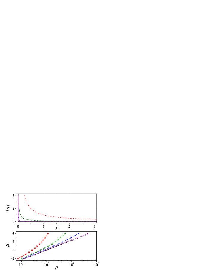
Figure 3: Top: Coulomb potential $U(x)=a/x$ for various values of the parameter $a$. Bottom: electrochemical potential versus particle density at temperature $T=1$. In both panels, from top to bottom, $a=1,10^{-1},10^{-2}$, and $10^{-4}$, respectively. The straight dashed line shows the analytical relation [Eq. (5)] between $\mu$ and $\rho$ for the hard-point gas.

For the computation of the thermopower and the thermal conductivity, we use Langevin heat baths  Dharrev set at temperatures $T_{L}=T+\Delta T/2$ and $T_{R}=T-\Delta T/2$. In our simulations, the value of $\Delta T$, 10% of $T$, is set with the consideration that it is small enough to guarantee the system to be in the linear response regime but meanwhile not too small to facilitate the simulations. (Random tests with smaller $\Delta T$, e.g., 4% of $T$ have been done and the same results have been obtained.) The system is evolved with velocity-Verlet algorithm, but we have verified that all the results do not depend on the integration algorithm. The relaxation stage is longer than $t=10^{7}$ for all the simulated cases.

With regard to the electrical conductivity, in this case it is not necessary to use the Green-Kubo formula. Indeed, thanks to momentum conservation, $\sigma$ is ballistic and can be computed analytically. Using a stochastic model of thermochemical baths carlos2001 ; carlos2003 , we have $j_{\rho}=\gamma_{L}-\gamma_{R}$, where $\gamma_{\alpha}=\rho_{\alpha}\sqrt{k_{B}T}/\sqrt{2\pi m}$ is the injection rate of particles from reservoir $\alpha$ into the system ($\alpha=L,R$ stands for the left and right reservoir, respectively), and $\rho_{\alpha}$ is the density of particles in reservoir $\alpha$, modeled as an infinite one-dimensional ideal gas. Since the electrochemical potential $\mu_{\alpha}$ for reservoir $\alpha$ is given by $\mu_{\alpha}=k_{B}T\ln(\lambda\rho_{\alpha})$ huang , we obtain $\gamma_{\alpha}=\frac{k_{B}T}{h}\exp(\beta\mu_{\alpha})$ and, therefore, within linear response regime, $j_{\rho}=\frac{\exp(\beta\mu_{\alpha})}{h}\,\Delta\mu$. The electrical conductivity is ballistic and given by $\sigma=GL$, with the conductance

$$G=\frac{ej_{\rho}}{\Delta\mu}=\frac{e}{h}\,\exp(\beta\mu),$$ (8)

where, always within linear response, $\mu\approx\mu_{L}\approx\mu_{R}$.

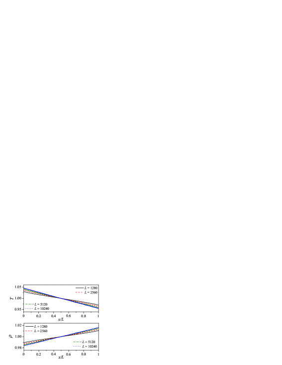
Figure 4: (Color online) Temperature (top panel) and the density (bottom panel) profiles for the Coulomb gas model. The temperatures of the two heat baths are set to be $T_{L}=1.05$ and $T_{R}=0.95$.

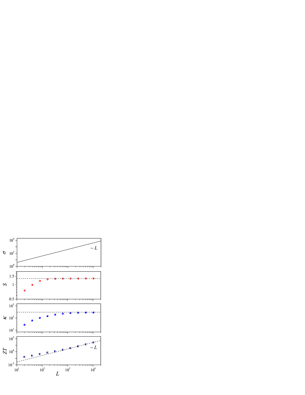
Figure 5: (Color online) Dependence of the transport coefficients $\sigma$, $S$, $\kappa$ and $ZT$ on the system size $L$ for the Coulomb gas model. Dashed lines are drawn for reference. The temperature $T=1$ and the interaction strength $a=1$.

Figure 4 shows the stationary temperature and density profiles for the Coulomb gas model. Similarly to the diatomic hard-point gas model, the system’s temperatures at the boundaries approach the temperatures of the thermal baths when the system size $L\to\infty$; i.e., $T^{\prime}_{L}\to T_{L}$ and $T^{\prime}_{R}\to T_{R}$. In Fig. 5 we show the transport coefficients $\sigma$, $S$, $\kappa$, and the thermoelectric figure of merit $ZT$. For $\sigma$ we plot the analytically determined linear growth as a function of the system size, $\sigma=GL$, with the conductance $G$ given by Eq. (8) (we have checked that consistent results, i.e., $\sigma\sim L$, can also be obtained by the Green-Kubo formula in equilibrium simulations, where the integration time is correctly truncated to take into account the ballistic transport Lepri03 ). The thermal conductivity increases for small system sizes and then saturates, as expected in a system that obeys the Fourier law. This behavior has been reported in recent investigations of several one-dimensional models of interacting particles Zhong12 ; chen ; dhar ; wang ; savin ; Fourierlike . While the Fourier-like regime might be an intermediate (in the system size) regime, followed by an asymptotic regime of anomalous thermal conductivity $\kappa\sim L^{1/3}$ Lepri03 ; Dharrev , its range may expand rapidly as an integrable limit (here, for $a\to 0$) is approached Fourierlike . As a consequence, for practical purposes we can assume that the system obeys the Fourier law. Since also the thermopower saturates as predicted for ballistic transport [see Eq. (13) in Sec. IV.3], we can conclude that $ZT$ grows linearly with the system size. In what follows, we show that the divergence of $ZT$ with the system size can be explained in terms of a general theoretical argument for momentum-conserving systems Benenti .

IV.3 Thermoelectricity in momentum-conserving systems

At the thermodynamic limit, the presence of nonzero Drude weights ${\cal D}_{ij}$ is a signature of ballistic transport zotos ; garst ; zotosreview ; heidrich-meisner ; i.e., the kinetic coefficients $L_{ij}$ scale linearly with the system size $L$. As a consequence, the thermopower $S$ is asymptotically size-independent. The finite-size Drude weights, for a system of size $L$, can be related to the existence of relevant conserved quantities of the system and computed by means of the Suzuki formula Suzuki . Such formula states that

$$\begin{array}[]{c}{\displaystyle C_{ij}(L)\equiv\lim_{t\to\infty}\frac{1}{t}\int_{0}^{t}dt^{\prime}\langle J_{i}(t^{\prime})J_{j}(0)\rangle_{T}}\\ \\ {\displaystyle~{}~{}=\sum_{n=1}^{M}\frac{\langle J_{i}Q_{n}\rangle_{T}\langle J_{j}Q_{n}\rangle_{T}}{\langle Q_{n}^{2}\rangle_{T}},}\end{array}$$ (9)

where $\langle\cdots\rangle_{T}$ denotes the thermal average at temperature $T$, and $\{Q_{n}$, $n=1,\cdots,M\}$ denote $M$ orthogonal constants of motion, which are relevant; that is, non-orthogonal to the considered currents, in our case to the currents $J_{\rho}$ and $J_{u}$: $\langle J_{\rho}Q_{n}\rangle_{T}\neq 0$ and $\langle J_{u}Q_{n}\rangle_{T}\neq 0$. The finite-size Drude weights are then defined as

$$D_{ij}(L)\equiv\frac{1}{2L}\,C_{ij}(L)\ .$$ (10)

If the thermodynamic limit $L\to\infty$ commutes with the long-time limit $t\to\infty$, then the thermodynamic Drude weights ${\cal D}_{ij}$ can be obtained as

$${\cal D}_{ij}=\lim_{L\to\infty}D_{ij}(L).$$ (11)

Moreover, if the limit does not vanish we can conclude that the presence of relevant conservation laws yields nonzero generalized Drude weights, which in turn implies ballistic transport.

We can see from Suzuki’s formula that for systems with a single relevant constant of motion ($M=1$), the ballistic contribution to $\det\mathbb{L}$ vanishes, since it is proportional to ${\cal D}_{\rho\rho}{\cal D}_{uu}-{\cal D}_{\rho u}^{2}$, which is zero from Eqs. (9), (10), and (11). Hence, $\det\mathbb{L}$ grows slower than $L^{2}$, and therefore the thermal conductivity $\kappa\sim\det{\mathbb{L}}/L_{\rho\rho}$ grows sub-ballistically, $\kappa\sim L^{\nu}$, with $\nu<1$. Furthermore, since $\sigma\sim L_{\rho\rho}\sim L$ is ballistic and $S\sim L^{0}$, we can conclude that Benenti

$$ZT=\frac{\sigma S^{2}}{\kappa}\,T\propto L^{1-\nu}\ .$$ (12)

Hence, $ZT$ diverges in the thermodynamic limit $L\to\infty$. This general theoretical argument applies, for instance, to systems where momentum is the only relevant conserved quantity. It has so far been illustrated in a toy model, i.e., a 1D dimerized gas of interacting hard-point particles Benenti , and in a two-dimensional stochastic model of interacting particles Benenti14 . Here we consider the more realistic and complex model of the Coulomb gas.

In order to check if our theory applies to the Coulomb gas model, in particular if the thermodynamic limit $L\to\infty$ commutes with the long-time limit $t\to\infty$, we need to compute the current correlation functions. For this aim we perform the equilibrium simulations with periodic boundary conditions. We prepare the equilibrium state of the system by using Andersen heat baths Andersen at the same given temperature $T$ and evolve the system for a sufficiently long time to make sure that it has been well thermalized. Then we remove the heat baths from the system. Starting from this moment the system is evolved isolatedly. After another long enough time of evolution, the correlation functions $\langle J_{i}(t)J_{j}(0)\rangle_{T}$ ($i,j=\rho,u$) are computed as functions of time.

Figure 6: (Color online) Current-current correlation functions for the Coulomb gas model at temperature $T=1$ and interaction strength $a=1$. In all the panels, the black straight lines are for $L=64$, the red dashed lines are for $L=128$, and green dash-dotted lines are for $L=256$. The results of the finite-size Drude weights $D_{ij}(L)$ by Suzuki’s formula (blue dotted horizontal line for $L=256$) are also shown for comparison.

The numerical results for the autocorrelation functions of $J_{\rho}$ and $J_{u}$, and for the cross correlation function between them are shown in Fig. 6. It can be seen that correlation function $\langle J_{u}(t)J_{u}(0)\rangle_{T}$ approaches a finite nonzero value as the correlation time increases and that the characteristic time scale to approach such value is independent of the system size. Other current-current correlation functions are constant. We have, therefore, a strong numerical evidence that we can commute the long-time limit $t\to\infty$ and the thermodynamic limit $L\to\infty$ and we can compute the thermodynamic Drude weights ${\cal D}_{ij}$ by means of Eq. (11). We also compute the finite-size Drude weights $D_{ij}(L)$ via the Suzuki formula Eqs. (9) and Eq. (10), and indicate its value by a dotted horizontal line in the plots of Fig. 6. (Note that it is not a function of time $t$.) The obtained numerical results are in good agreement with the (asymptotical) values of the correlation functions. We note that $\langle J_{\rho}(t)J_{\rho}(0)\rangle_{T}$ does not decay; this is because $J_{\rho}=P/m$ is a conserved quantity, so that the particle current is the same as for the ideal gas, and therefore by employing the Suzuki’s formula, we can analytically obtain that $D_{\rho\rho}=T\rho/2$. This result is in perfect agreement with the data shown in the last panel of Fig. 6. In fact, $\langle J_{\rho}(t)J_{u}(0)\rangle_{T}=P\langle J_{u}(0)\rangle_{T}/m$ is also trivially constant due to momentum conservation. (See the middle panel of Fig. 6). Finally, as expected from the theory Benenti , $D_{\rho\rho}(L)D_{uu}(L)-D_{\rho u}^{2}(L)=0$; this is also verified for various system sizes.

For momentum-conserving systems, we can also compute the asymptotic value of the thermopower (as $L\to\infty$) based on theoretical prediction for ballistic transport:

$$S=\frac{1}{eT}\left(\frac{{\cal D}_{\rho u}}{{\cal D}_{\rho\rho}}-c\right).$$ (13)

Here, ${\cal D}_{ij}$ can be obtained with the above equilibrium simulations via Eq. (11), and $c$ is a numerical constant that can be determined by comparison with the results obtained by the grand-canonical Monte Carlo method foot_mu .

V Conclusions

Starting from the definition of thermopower as a measure of the magnitude of an induced thermoelectric voltage in response to a temperature difference and taking advantage of the grand canonical Monte Carlo method to connect the particle density to the electrochemical potential, we are able to compute the thermoelectric coefficients in systems with more general interaction than the instantaneous collisions. As a physically significant illustration of our approach, we have shown that for classical one-dimensional, momentum-conserving systems with (screened) Coulomb interaction, the thermoelectric figure of merit increases, on a broad range of the system size, linearly. In principle, our strategy can be applied without restrictions on the type of interaction, even in the case of electron-lattice coupling, hence it could be useful for studying thermoelectricity in more complex and realistic systems.

Appendix A Grand-canonical Monte Carlo simulations

For a given electrochemical potential, system size, and temperature, the grand-canonical Monte Carlo method samples the grand-canonical probability distribution

$$f_{\mu LT}({\bf x}^{N};N)\propto\frac{L^{N}\exp(\beta\mu N)}{N!\,\lambda^{N}}\exp[-\beta\mathcal{U}({\bf x}^{N})],$$ (14)

where $\lambda$ is the de Broglie thermal wavelength and $\mathcal{U}$ is the potential energy for the $N$-particle configuration ${\bf x}^{N}=(x_{1},...,x_{N})$. Our simulations are performed along the following steps (for a detailed description of the grand-canonical Monte Carlo method see Ref. DFrenkel ):

1. Start from an initial state with random positions of $N$ particles;

2. A random displacement is applied to a particle selected at random. This move is accepted with probability

$$\min\{1,\exp[-\beta({\mathcal{U}}_{\rm new}-{\mathcal{U}}_{\rm old})]\},$$ (15)

where ${\mathcal{U}}_{\rm old}$ and ${\mathcal{U}}_{\rm new}$ denote, here and in the following, the potential energy before and after the move, respectively;

3. The creation of a new particle at a random position is accepted with a probability

$$\min\left\{1,\frac{L}{\lambda(N_{\rm old}+1)}\exp[-\beta({\mathcal{U}}_{\rm new}-{\mathcal{U}}_{\rm old})]\right\},$$ (16)

where $N_{\rm old}$ denotes, here and in the following, the particle number before the move;

4. The removal of a randomly selected particle is accepted with a probability

$$\min\left\{1,\frac{\lambda N_{\rm old}}{L}\exp[-\beta({\mathcal{U}}_{\rm new}-{\mathcal{U}}_{\rm old})]\right\};$$ (17)

5. Repeat steps 2 to 4, for a long enough time to reach the equilibrium state.

6. Repeat steps 2 to 4, to have a sufficient number of microstates to compute the average number of particles $\langle N\rangle$ and the density $\rho=\langle N\rangle/L$ with good accuracy.

Note that this algorithm obeys the detailed balance principle and therefore leads to a random sampling of the grand-canonical probability distribution DFrenkel .

References

- (1) M. S. Dresselhaus, G. Chen, M. Y. Tang, R. G. Yang, H. Lee, D. Z. Wang, Z. F. Ren, J. -P. Fleurial, and P. Gogna, Adv. Mater. 19, 1043 (2007).
- (2) G. J. Snyder and E. S. Toberer, Nature Mater. 7, 105 (2008).
- (3) A. Shakouri, Annu. Rev. Mater. Res. 41, 399 (2011).
- (4) Y. Dubi and M. Di Ventra, Rev. Mod. Phys. 83, 131 (2011).
- (5) G. Benenti, G. Casati, T. Prosen, and K. Saito, arXiv:1311.4430.
- (6) C. Kittel, Introduction to Solid State Physics, 8th ed. (John Wiley & Sons, New York, 2005).
- (7) G. D. Mahan and J. O. Sofo, Proc. Natl. Acad. Sci. USA 93 7436 (1996).
- (8) T. E. Humphrey, R. Newbury, R. P. Taylor, and H. Linke, Phys. Rev. Lett. 89 116801 (2002).
- (9) T. E. Humphrey and H. Linke, Phys. Rev. Lett. 94 096601 (2005).
- (10) G. Benenti, G. Casati, and J. Wang, Phys. Rev. Lett. 110, 070604 (2013).
- (11) J. Wang, G. Casati, T. Prosen, and C.-H. Lai, Phys. Rev. E 80, 031136 (2009).
- (12) S. Lepri, R. Livi, and A. Politi, Phys. Rep. 377, 1 (2003).
- (13) A. Dhar, Adv. Phys. 57, 457 (2008).
- (14) D. Frenkel and B. Smit, Understanding Molecular Simulation: From Algorithms to Applications, 2nd ed. (Academic Press, San Diego, 2001), Chap. 5.
- (15) R. Kubo, M. Toda, and N. Hashitsume, Statistical Physics II, in Springer Series in Solid-State Sciences, vol. 31 (Springer, Berlin, 1991).
- (16) G. Casati, Found. Phys. 16, 51 (1986).
- (17) G. Benenti, G. Casati, and C. Mejía-Monasterio, New J. Phys. 16, 015014 (2014).
- (18) Y. Zhong, Y. Zhang, J. Wang, and H. Zhao, Phys. Rev. E 85, 060102(R) (2012).
- (19) S. Chen, Y. Zhang, J. Wang, and H. Zhao, arXiv: 1204.5933.
- (20) S. G. Das, A. Dhar, and O. Narayan, J. Stat. Phys. 154, 204 (2013).
- (21) L. Wang, B. Hu, and B. Li, Phys. Rev. E 88, 052112 (2013).
- (22) A. V. Savin and Y. A. Kosevich, Phys. Rev. E 89, 032102 (2014).
- (23) S. Chen, J. Wang, G. Casati, and G. Benenti. Phys. Rev. E 90, 032134 (2014).
- (24) H.B. Callen, Thermodynamics and an Introduction to Thermostatics, 2nd ed. (John Wiley & Sons, New York, 1985).
- (25) S. R. de Groot and P. Mazur, Nonequilibrium Thermodynamics (North-Holland, Amsterdam, 1962).
- (26) A. Dhar, Phys. Rev. Lett. 86, 3554 (2001).
- (27) A. V. Savin, G. P. Tsironis, and A. V. Zolotaryuk, Phys. Rev. Lett. 88, 154301 (2002).
- (28) P. Grassberger, W. Nadler, and L. Yang, Phys. Rev. Lett. 89, 180601 (2002).
- (29) G. Casati and T. Prosen, Phys. Rev. E 67, 015203 (2003).
- (30) P. Cipriani, S. Denisov, and A. Politi, Phys. Rev. Lett. 94, 244301 (2005).
- (31) V. Zaburdaev, S. Denisov, and P. Hänggi, Phys. Rev. Lett. 106, 180601 (2011).
- (32) S. Chen, Y. Zhang, J. Wang, and H. Zhao, Phys. Rev. E 87, 032153 (2013).
- (33) S. Chen, Y. Zhang, J. Wang, and H. Zhao, Sci. China-Phys. Mech. Astron. 56, 1466 (2013).
- (34) S. Chen, Y. Zhang, J. Wang, and H. Zhao, Phys. Rev. E 89, 022111 (2014).
- (35) C. B. Mendl and H. Spohn, Phys. Rev. E 90, 012147 (2014).
- (36) K. Huang, Statistical Mechanics (2nd ed.), (John Wiley & Sons, New York, 1987).
- (37) J. L. Lebowitz and H. Spohn, J. Stat. Phys. 19, 633 (1978); R. Tehver, F. Toigo, J. Koplik, and J. R. Banavar, Phys. Rev. E 57, R17 (1998).
- (38) C. Mejía-Monasterio, H. Larralde, and F. Leyvraz, Phys. Rev. Lett. 86, 5417 (2001).
- (39) H. Larralde, F. Leyvraz, and C. Mejía-Monasterio, J. Stat. Phys. 113, 197 (2003).
- (40) X. Zotos, F. Naef, and P. Prelovšek, Phys. Rev. B 55, 11029 (1997).
- (41) X. Zotos and P. Prelovšek, in Strong Interactions in Low Dimensions, edited by D. Baeriswyl and L. Degiorgi (Kluwer Academic Publishers, Dordrecht, 2004).
- (42) M. Garst and A. Rosch, Europhys. Lett. 55, 66 (2001).
- (43) F. Heidrich-Meisner, A. Honecker, and W. Brenig, Phys. Rev. B 71, 184415 (2005).
- (44) M. Suzuki, Physica (Amsterdam) 51, 277 (1971).
- (45) H. C. Andersen, J. Chem. Phys. 72, 2384 (1980).
- (46) For the case of the hard-point gas model Benenti , we found agreement between the results by the two methods, provided we set , where is the electrochemical potential obtained from the grand-canonical Monte Carlo method. Indeed, for the hard-point gas the dependence of on and is the same as that of the ideal gas used as reservoir in the grand-canonical Monte Carlo method. In general (and in particular for the case of Coulomb interaction) the constant has not the meaning of electrochemical potential; still it can be determined by comparison with the Monte Carlo results.