Jumping Neptune Can Explain the Kuiper Belt Kernel

Abstract

The Kuiper belt is a population of icy bodies beyond the orbit of Neptune. A particularly puzzling and up-to-now unexplained feature of the Kuiper belt is the so-called ‘kernel’, a concentration of orbits with semimajor axes $a\simeq 44$ AU, eccentricities $e\sim 0.05$, and inclinations $i<5^{\circ}$. Here we show that the Kuiper belt kernel can be explained if Neptune’s otherwise smooth migration was interrupted by a discontinuous change of Neptune’s semimajor axis when Neptune reached $\simeq 28$ AU. Before the discontinuity happened, planetesimals located at $\sim$40 AU were swept into Neptune’s 2:1 resonance, and were carried with the migrating resonance outwards. The 2:1 resonance was at $\simeq$44 AU when Neptune reached $\simeq 28$ AU. If Neptune’s semimajor axis changed by fraction of AU at this point, perhaps because Neptune was scattered off of another planet, the 2:1 population would have been released at $\simeq$44 AU, and would remain there to this day. We show that the orbital distribution of bodies produced in this model provides a good match to the orbital properties of the kernel. If Neptune migration was conveniently slow after the jump, the sweeping 2:1 resonance would deplete the population of bodies at $\simeq$45-47 AU, thus contributing to the paucity of the low-inclination orbits in this region. Special provisions, probably related to inefficiencies in the accretional growth of sizable objects, are still needed to explain why only a few low-inclination bodies have been so far detected beyond $\simeq$47 AU.

1 Introduction

Following the pioneering work of Malhotra (1993, 1995), studies of Kuiper belt dynamics first considered the effects of outward migration of Neptune that can explain the prominent populations of Kuiper Belt Objects (KBOs) in major resonances (Hahn & Malhotra 1999, 2005; Chiang & Jordan 2002; Chiang et al. 2003; Levison & Morbidelli 2003; Gomes 2003; Murray-Clay & Chiang 2005, 2006). With the advent of the notion that the early Solar System may have suffered a dynamical instability (Thommes et al. 1999, Tsiganis et al. 2005, Morbidelli et al. 2007), the focus broadened, with the more recent theories invoking a transient phase with an eccentric orbit of Neptune (Levison et al. 2008, Morbidelli et al. 2008, Batygin et al. 2011, Wolff et al. 2012, Dawson & Murray-Clay 2012).

The consensus emerging from these studies is that the hot classical, resonant, scattered and detached populations (see Gladman et al. 2008 for the definition of these groups), formed in a massive planetesimal disk at $\lesssim$30 AU, and were dynamically scattered to their current orbits by migrating (and possibly eccentric) Neptune. The wide inclination distribution of the implanted populations indicates that Neptune’s migration was long range and relatively slow, such that there was enough time for various processes to excite the orbital inclinations (Nesvorný 2015).

The Cold Classicals (hereafter CCs), on the other hand, have low orbital inclinations ($i<5^{\circ}$) and several physical properties (ultra red colors, large binary fraction, steep size distribution of large objects, relatively high albedos) that distinguish them from all other KBO populations. The most straightforward interpretation of these properties is that the CCs formed and/or dynamically evolved by different processes than other trans-Neptunian populations. Here we consider the possibility that the CCs formed at $>$40 AU and survived Neptune’s early ‘wild days’ relatively unharmed (Batygin et al. 2011, Wolff et al. 2012).

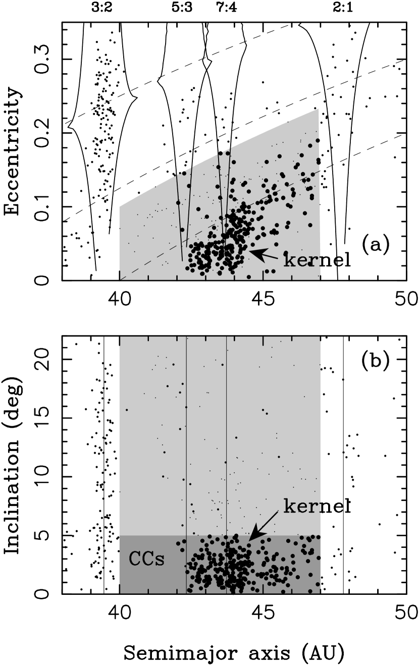
Figure 1: The orbital elements of the KBOs observed in three or more oppositions. Various dynamical classes are highlighted. The CCs with $i<5^{\circ}$ are denoted by larger symbols. The solid lines in panel (a) follow the borders of important mean motion resonances. The low-inclination orbits with $40<a<42$ AU are unstable due to the secular resonance overlap ($\nu_{7}$ and $\nu_{8}$; Kněžević 1991, Duncan et al. 1995). The location of the Kuiper belt kernel is indicated by arrows.

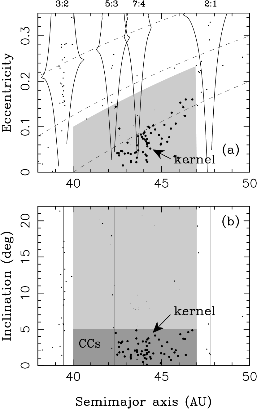
Figure 2: The orbital elements of the KBOs detected by the CFEPS. The CFEPS is one of the largest surveys with published characterization (currently 169 objects; Petit et al. 2011). Various dynamical classes are highlighted. The CCs with $i<5^{\circ}$ are denoted by larger symbols. The solid lines in panel (a) follow the borders of important mean motion resonances. The location of the Kuiper belt kernel is indicated by arrows.

According to Petit et al. (2011), the CC population can be divided into the ‘stirred’ and ‘kernel’ components. The stirred orbits have the semimajor axes $42<a<47$ AU, inclinations $i<5^{\circ}$, and small eccentricities with an upper limit that raises from $e\simeq 0.05$ for $a=42$ AU to $e\simeq 0.15$ for $a=47$ AU. The kernel is a narrow concentration of low-inclination orbits with $a\simeq 44$ AU, $e\sim 0.05$, and a $\simeq$0.5-1 AU width in the semimajor axis. Figures 1 and 2 illustrate the observed distribution of orbits. According to the Canada-France Ecliptic Plane Survey (CFEPS; Kavelaars et al. 2008), the number of KBOs in the kernel with absolute magnitude $H<8$ is $900\pm 200$, which is roughly one third of the number of stirred objects with $H<8$ (Petit et al. 2011). The kernel is therefore an important component of the Kuiper belt (see also Jewitt et al. 1996).

Chiang (2002) and Chiang et al. (2003) discussed the possibility that the concentration of bodies near 44 AU is a collisional family (see, e.g., Nesvorný et al. 2015 for a recent review of collisional families in the asteroid belt). One problem with this hypothesis is that the collisional families in the Kuiper belt are expected to be stretched over many AUs in the semimajor axis (due to a relatively large contribution of the ejection speed to the orbital motion; Marcus et al. 2011). Also, the relatively large number of $H<8$ objects in the kernel implies that the parent body of the putative family would have to be a dwarf planet at least as large as Pluto. The family hypothesis therefore seems to be improbable.

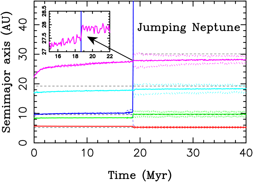
Figure 3: The orbit histories of the giant planets in an instability simulation from NM12. In this example, the fifth giant planet was initially placed on an orbit between Saturn and Uranus and was given a mass equal to the Neptune mass. Ten thousand particles, representing the outer planetesimal disk, were distributed with the semimajor axis $23.5<a<29$ AU, surface density $\Sigma=1/a$, and low eccentricity and low inclination. With the total disk mass $M_{\rm disk}=15$ $M_{\rm Earth}$, each disk particle has $\simeq$0.75 Pluto mass. The plot shows the semimajor axes (solid lines), and perihelion and aphelion distances (thin dashed lines) of each planet’s orbit in a time frame $\pm 20$ Myr around the instability. Neptune migrates into the outer disk during the first stage of the simulation. It reaches $\simeq$27.5 AU when the instability happens ($t\simeq 18.3$ Myr). During the instability, Neptune has a close encounter with the fifth planet and its semimajor axis jumps by $\simeq$0.4 AU outward (see the inset). The fifth planet is subsequently ejected from the solar system by Jupiter. Neptune’s migration after the instability can be approximated with the e-folding timescale $\tau_{2}=50$ Myr. The final orbits of the four remaining planets are a good match to those in the present Solar System (thin dashed lines).

If not a family than what is the kernel? Motivated by this question, here we consider the possibility that the kernel is a population of bodies that was captured into, and subsequently released from Neptune’s 2:1 resonance. Our recent simulations of the planetary migration/instability in Nesvorný & Morbidelli (2012, hereafter NM12) provide the right framework for this model. The NM12 simulations are characterized by the first, faster migration stage during which Neptune reached $\simeq 28$ AU, followed by a dynamical instability, when planetary encounters happened, followed by the second, very slow migration stage during which Neptune reached $30$ AU (Fig. 3).

We find that bodies originally at $\sim$40 AU can be captured into the 2:1 resonance during the first migration stage before the instability. The 2:1 resonance is at $\simeq$44 AU if the instability happens when Neptune is at $\simeq 28$ AU. We have looked into various cases from NM12 and found that the semimajor axis of Neptune discontinuously changes during the instability, due to the effect of planetary encounters, by $\simeq$0.2-0.5 AU (Fig. 3). Consequently, the 2:1 resonance is expected to jump by $\simeq$0.3-0.75 AU, which exceeds the full width of the 2:1 resonance for $e<0.1$. It is therefore expected in this model that resonant bodies with $e<0.1$ are released at $\simeq$44 AU, where they would remain to the present time.

2 The Integration Method

Our numerical integrations consist in tracking the orbits of four planets (Jupiter to Neptune) and a large number of test particles representing the outer planetesimal disk. To set up an integration, Jupiter, Saturn and Uranus were placed on their current orbits. Neptune was placed on an orbit with the semimajor axis $a_{\rm N,0}$, eccentricity $e_{\rm N,0}$, and inclination $i_{\rm N,0}$. These elements define the Neptune orbit before the main stage of migration/instability. In most of our simulations we used $a_{\rm N,0}=24$ AU, because the wide inclination distribution of the hot, resonant and detached population requires that Neptune’s migration was long range ($a_{\rm N,0}\lesssim 25$ AU; Nesvorný 2015), $e_{\rm N,0}=0$ and $i_{\rm N,0}=0^{\circ}$. The swift_rmvs4 code (Levison & Duncan 1994) was used to follow the evolution of planets and disk particles. The code was modified to include fictitious forces that mimic the radial migration and damping. These forces were parametrized by the exponential e-folding timescales, $\tau_{a}$, $\tau_{e}$ and $\tau_{i}$, where $\tau_{a}$ controls the radial migration rate, and $\tau_{e}$ and $\tau_{i}$ control the damping rate of $e$ and $i$. Here we set $\tau_{a}\sim\tau_{e}\sim\tau_{i}$ $(=\tau_{1})$, because such roughly comparable timescales were suggested by previous work.

The numerical integrations of the first migration stage were stopped when Neptune reached $a_{\rm N,1}=27.8$ AU. Then, to approximate the effect of planetary encounters during the instability, we applied a discontinuous change of Neptune’s semimajor axis and eccentricity, $\Delta a_{\rm N}$ and $\Delta e_{\rm N}$. In reality, we find from NM12 that Neptune may suffer up to several close encounters with another planet, and that the evolution of $a_{\rm N}$ and $e_{\rm N}$ may be complex, with two (or more) encounters significant contributing to the overall change of $a_{\rm N}$ and $e_{\rm N}$. Studying such evolution histories with multiple changes of $a_{\rm N}$ and $e_{\rm N}$ is left for future work. Here we focus on a simple case where the overall change is approximated by a single event. Motivated by the NM12 results, we set $\Delta a_{\rm N}=0$, 0.25, 0.5 or 0.75 AU, and $\Delta e_{\rm N}=0$, 0.05, 0.1, or 0.15. The purpose of $\Delta a_{\rm N}=\Delta e_{\rm N}=0$ is to have a reference case for the comparison purposes. No change is applied to the orbital inclination of Neptune, because an inclination change should not critically affect the processes studied here. [The excitation of Neptune’s orbital inclination seen in the NM12 simulations is typically not large enough to explain why the CCs have an inclination distribution with the characteristic width of $\simeq 2^{\circ}$ (Brown 2001).]

The second migration stage starts with Neptune having the semimajor axis $a_{\rm N,2}=a_{\rm N,1}+\Delta a_{\rm N}$. We apply the swift_rmvs4 code, and migrate the semimajor axis (and damp the eccentricity) on an e-folding timescale $\tau_{2}$. By fine tuning the migration amplitude the final semimajor axis of Neptune was adjusted to be within 0.05 AU of its current mean $a_{\rm N}=30.11$ AU, and the orbital period ratio, $P_{\rm N}/P_{\rm U}$, where $P_{\rm N}$ and $P_{\rm U}$ are the orbital periods of Neptune and Uranus, was adjusted to end up within 0.5% of its current value ($P_{\rm N}/P_{\rm U}=1.96$). A strict control over the final orbits of planets is important, because it guarantees that the mean motion and secular resonances in the Kuiper belt region have the correct locations. All simulations were run to 1 Gyr. The interesting cases were extended to 4 Gyr with the standard swift_rmvs4 code (i.e., without migration/damping in the 1-4 Gyr interval).

As for the specific values of $\tau_{1}$ and $\tau_{2}$ used in our integrations, we found from NM12 that the orbital behavior of Neptune can be approximated by $\tau_{1}\simeq 10$ Myr and $\tau_{2}\simeq 30$ Myr for a disk mass $M_{\rm disk}=20$ $M_{\rm Earth}$, and $\tau_{1}\simeq 20$ Myr and $\tau_{2}\simeq 50$ Myr for a disk mass $M_{\rm disk}=15$ $M_{\rm Earth}$ (these masses refer to the massive disk at $<30$ AU; below we consider a low-mass continuation of this disk beyond 30 AU). Slower migration rates are possible for lower disk masses. Moreover, we find that the real migration is not precisely exponential with the effective $\tau$ being longer than the values quoted above during the very late migration stages ($\tau\gtrsim 100$ Myr). This is consistent with constraints from Saturn’s obliquity, which was presumably exited by late, near-adiabatic capture in a spin-orbit resonance (e.g., Vokrouhlický & Nesvorný 2015). Much shorter migration timescales than those quoted above do not probably apply, because they would violate constraints from the wide inclination distribution of the hot classical and resonant populations (Nesvorný 2015). Here we therefore use $\tau_{1}=10$ Myr or 30 Myr, $\tau_{2}=30$ or 100 Myr, and also test a case with $\tau_{2}=200$ Myr.

Each simulation included 5,000 disk particles distributed from 30 to 50 AU. Their radial profile was set such that the disk surface density $\Sigma\propto 1/r$, where $r$ is the heliocentric distance. There is therefore an equal number of particles (250) in each radial AU. A larger resolution is not needed, because a significant fraction of particles in the CC region (42-47 AU) survive, and the final statistics is therefore good enough to perform a careful comparison with observations. The disk particles were assumed to be massless such that their gravity does not interfere with the migration/dumping routines. The fate of the massive disk at $<30$ AU was not studied here, because the implantation of bodies from $<30$ AU into the Kuiper belt was investigated elsewhere (e.g., Levison et al. 2008, Dawson & Murray-Clay 2012, Nesvorný 2015).

An additional uncertainty relates to the dynamical structure of the original planetesimal disk at 30-50 AU. Here we operate under the assumption that the disk was dynamically cold with the low orbital eccentricities and low orbital inclinations. Since Neptune’s inclination remains small in our simulations, we do not identify any dynamical effects that could significantly influence the orbital inclinations in the 42-47 AU region (passing mean motion resonances do not affect inclinations much). The initial inclinations distribution was therefore chosen to be similar to that inferred for the present population of the CCs from observations. Specifically, we used $N(i)\,{\rm d}i=\sin i\exp(-i^{2}/2\sigma_{i}^{2})\,{\rm d}i$, with $\sigma_{i}=2^{\circ}$ (Brown 2001, Gulbis et al. 2010). The interaction of bodies with migrating mean motion resonances is known to depend on their orbital eccentricity, with low eccentricities more likely resulting in capture. The choice of the orbital eccentricity distribution could therefore, in principle, affect the results. The initial eccentricities in our simulations were distributed according to the Rayleigh distribution with $\sigma_{e}=0.01$, 0.05 or 0.1, where $\sigma_{e}$ is the usual scale parameter of the Rayleigh distribution (the mean of the Rayleigh distribution is equal to $\sigma_{e}\sqrt{\pi/2}$). Studying cases with larger eccentricity values would not be useful, because most main belt orbits with $e>0.1$ are dynamically unstable.

3 Results

We first discuss a reference simulation to illustrate the suggested relationship between the 2:1 resonance population deposited at $\simeq$44 AU during Neptune’s jump, and the Kuiper belt kernel. Then, in Section 3.2, we explain how the results differ from the reference case when various model parameters are varied. The orbital distribution of the CC orbits beyond 45 AU is discussed in Section 3.3. Finally, in Section 3.4, we deal with the orbital dynamics of bodies below 40 AU, including the population captured in the 3:2 resonance. We show that the 3:2 population captured from the initial orbits with $a>30$ AU should represent only a small fraction ($\sim 1$%) of all Plutinos.

3.1 A Reference Case

Figure 4 shows the final distribution of orbits in the reference case with $a_{\rm N,0}=24$ AU, $\tau_{1}=30$ Myr, $a_{\rm N,1}=27.8$ AU, $\Delta a_{\rm N}=0.5$ AU, $\Delta e_{\rm N}=0.05$, $\tau_{2}=100$ Myr, and $\sigma_{e}=0.01$. This distribution can be compared to Figure 5, but we caution that Figure 5 contains observational biases while Figure 4 does not. Also, in Figure 4 we highlight with larger symbols all final orbits with $42<a<47$ AU and $q=a(1-e)>36$ AU, while to highlight an orbit in Figure 5 we also require that $i<5^{\circ}$ (to filter out the hot classicals).

The distributions of orbits in Figures 5 and 4 share several similarities, but also show several important differences. First, the model distribution of the CC orbits in Figure 4 is clustered at $a\simeq 44$ AU and $e<0.1$. This is the orbital location of the kernel. In the model, the concentration of orbits was created by the 2:1 resonance, which collected captured bodies before Neptune’s jump, and then released them with $a\simeq 44$ AU and $e<0.1$, when Neptune jumped. This can be conveniently demonstrated by comparing these model results with a simulation where $\Delta a_{\rm N}=0$. Figure 6 shows a comparison of various semimajor axis distributions. The observed distribution raises from below 42 AU, where very few low-inclination object exist due to the presence of overlapping secular resonances, toward the location of the kernel at $\simeq$44 AU. The model distribution obtained with $\Delta a_{\rm N}=0.5$ AU reproduces this trend very well, while that with $\Delta a_{\rm N}=0$ AU does not. This happens essentially because no concentration of orbits is created at $\simeq$44 AU if Neptune migrates smoothly, that is without a jump.

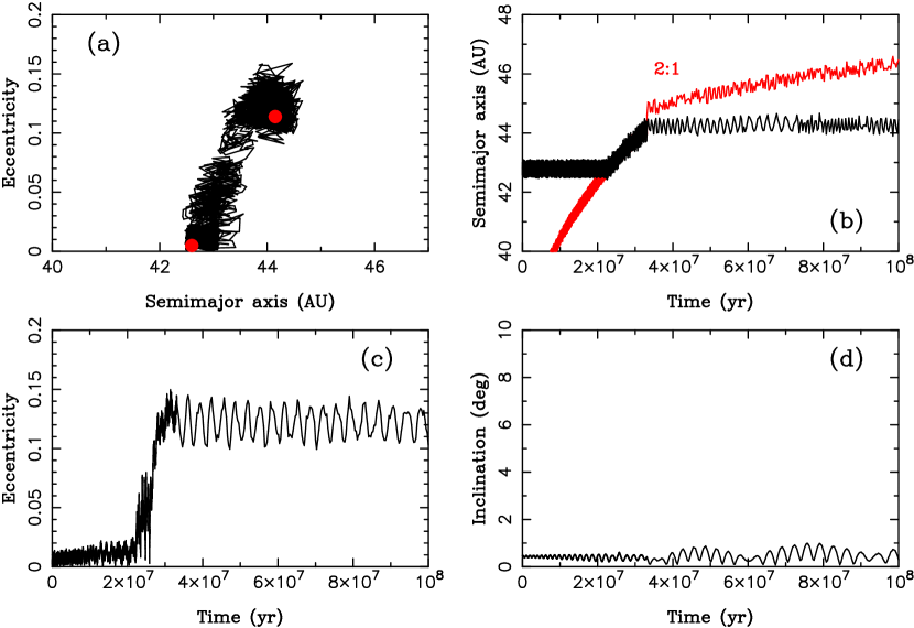
Figure 7: The orbital history of a test particle that was released from the 2:1 resonance when Neptune jumped (at $t=32.5$ Myr) The panels show: the (a) path of the disk particle in the $(a,e)$ projection; the two red dots show the initial and final orbits, (b) semimajor axis, (c) eccentricity, and (d) inclination. From $t\simeq 22$ Myr to $t\simeq 32$ Myr, the 2:1 resonance angle, $\sigma_{2:1}=2\lambda-\lambda_{\rm N}-\varpi_{\rm N}$, librates with a full amplitude of $\simeq 200^{\circ}$.

Figure 7 shows an example of orbit taken from our simulation with $\Delta a_{\rm N}=0.5$ AU. This example illustrates how an objects starting below 43 AU is captured by the the 2:1 resonance, which transports it to $\simeq$44 AU, where the body is released from the resonance during Neptune’s jump. This is a typical evolution path followed by bodies deposited into the kernel region in our simulations.

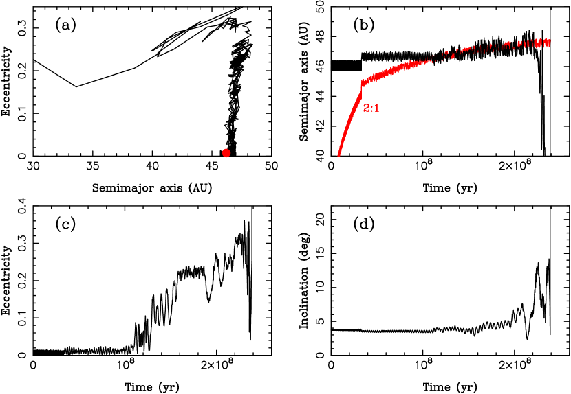
Figure 8: The orbital history of a test particle that started with $a\simeq 46$ AU and was destabilized by the 2:1 resonance. The panels show: the (a) path of the disk particle in the $(a,e)$ projection; the red dot shows the initial orbit, (b) semimajor axis, (c) eccentricity, and (d) inclination. The particle was captured into the 2:1 resonance at $t\simeq 110$ Myr after the start of the simulation. It remained on a resonant orbit with a very large libration amplitude to $t\simeq 220$ Myr, and subsequently evolved on a Neptune-crossing orbit.

The distribution of orbits for $a\gtrsim 45$ AU presents a challenge. The semimajor axis distribution of the observed orbits in Figures 5 and 6 sharply drops from 44 AU to 45 AU. The density of known low-$i$ orbits between 45 and 47 AU is roughly 15-30% lower than the peak value at 44 AU. This is often described as the Kuiper belt “edge” or “cliff” (Bernstein et al. 2004). The edge is not well reproduced in our simulations. The model density obtained with $\tau_{2}=100$ Myr drops only to $\simeq$50-60% of the peak value. In the model, the depletion is caused by a slowly migrating 2:1 resonance that captures and removes bodies from this region (see Figure 8 for an illustration). To obtain a better agreement, one would thus either need to create a stronger concentration of orbits at $\simeq$44 AU, such that the contrast increases by a factor of two or so, or produce a more severe depletion in the 45-47 AU region.

While this could be potentially achieved by slowing down the migration (see Section 3.2), a more fundamental problem with the result in Figure 4 is that the 2:1 resonance captures objects from the 45-47 AU region and becomes overpopulated, relative to observations, at the end of the simulation (see the clump of low-$i$ resonant orbits at $\simeq 48$ AU in Figure 4). This happens because only some of the orbits captured in the 2:1 resonance become destabilized later, as in Figure 8. Most captured orbits are stable and survive inside the resonance. Also, the low-$i$ and low-$e$ orbits beyond the 2:1 resonance ($a\gtrsim 49$ AU) remain practically unchanged in our simulations, while no bodies on such orbits were detected so far. We discuss this problem in Section 3.3.

3.2 Dependence on Model Parameters

Here we discuss the dependence of the results on: (1) $\Delta e_{\rm N}$ (Figure 9), (2) $\Delta a_{\rm N}$ (Figure 10), (3) $\tau_{1}$ and $\tau_{2}$ (Figure 11), and (4) the initial eccentricities of particles in the 30-50 AU region (Figure 12).

As for (1), we used $\Delta e_{\rm N}=0$, 0.05, 0.1 and 0.15. The results for $\Delta e_{\rm N}=0.05$ were discussed in the previous section. Figure 9 illustrates the result for the same model parameters as in the previous section, but $\Delta e_{\rm N}=0.1$. In this case, the kernel population obtained with $\Delta a=0.5$ AU (right panels in Fig. 9) is somewhat more concentrated near 44 AU than it was in Figure 4. The origin of this difference is not understood. It may have something to do with with the dynamics of large libration amplitude orbits inside the 2:1 resonance, and its dependence on $e_{\rm N}$. With $\Delta e_{\rm N}=0.1$ the kernel orbits obtained in the model have the semimajor axis between 43.8 and 44.6 AU, and eccentricity between 0.03 and 0.09, in a very close match to the distribution of the kernel orbits inferred from the CFEPS observations (Petit et al. 2011; their Figure 4). The left panels in Fig. 9 show that the kernel does not form if Neptune does not jump, as expected.

The results obtained with $\Delta e_{\rm N}=0$ (and $\Delta a_{\rm N}=0.5$ AU) also show the formation of the kernel, but in this case, if $\sigma_{e}=0.01$, a low-$e$ segment of the original disk survives at 44-45 AU. These orbits are not altered by the 2:1 resonance, which just jumps over them. Since such orbits are not observed, either $\Delta e_{\rm N}>0$ or $\sigma_{e}>0.01$. The case with $\Delta e_{\rm N}=0.15$ also does not apply, because the CC population at 42-45 AU is disrupted when Neptune’s eccentricity becomes large (here we used $\tau_{2}=100$ Myr; shorter migration timescales could work better with $\Delta e_{\rm N}=0.15$, but see Wolff et al. (2012), Dawson & Murray-Clay (2012), and Morbidelli et al. (2014)). This tests indicate that the preferred value for the eccentricity change of Neptune’s orbit is $\Delta e_{\rm N}\simeq 0.05$-0.1.

As for (2), Figure 10 shows the result for $\Delta a_{\rm N}=0.25$ AU and 0.75 AU ($\Delta e_{\rm N}=0.1$ and $\tau_{2}=100$ Myr). The case with $\Delta a_{\rm N}=0.25$ AU is within the range of the NM12 results, while in the one with $\Delta a_{\rm N}=0.75$ AU, Neptune’s jump is probably too large to be realistic (the cases with $\Delta a_{\rm N}>0.5$ AU do not happen too often in NM12). We used $\Delta a_{\rm N}=0.75$ AU just in case some future modification of the NM12 simulation setup would lead to a larger jump of Neptune. The results obtained here for $\Delta a_{\rm N}=0.25$ AU do not lead to the formation of the kernel (Figure 10, left panels), and are in fact very similar to those obtained with $\Delta a_{\rm N}=0$. The ones obtained with $\Delta a_{\rm N}=0.75$ AU, on the other hand, are very similar to the previous case with $\Delta a_{\rm N}=0.5$ AU, where a well-defined kernel forms. We conclude that the kernel constraint requires that Neptune’s semimajor axis changed by $\simeq$0.5-0.75 AU (with the lower values in this range being more in line with the NM12 results).

Figure 11 illustrates the dependence of the results on the migration timescale. Here we assumed that $\tau_{1}=10$ Myr and $\tau_{2}=30$ Myr, and left all other model parameters from Figure 9 unchanged. These shorter migration timescales would be more appropriate if Neptune’s migration was driven by a more massive planetesimal disk. The results are similar to those obtained for longer migration timescales. The kernel forms for $\Delta a=0.5$ AU and does not form for $\Delta a=0$. The compact orbital structure of the kernel obtained for $\Delta a=0.5$ AU is very similar to that obtained in the case with the longer migration timescales. This shows that the results are not sensitive to the migration timescale of Neptune. A minor difference between Figures 11 and 9 can be noticed in the 45-47 AU region, where the population of orbits is less depleted if the migration is faster. This is related to the migration-speed dependence of the removal by the 2:1 resonance. With $\tau_{2}=200$ Myr, which was the longest migration timescale considered here, only $\sim$32% of bodies survived in the 45-47 AU region (while 74% survived for $\tau_{2}=30$ Myr, and 47% survived for $\tau_{2}=100$ Myr).

Finally, we simulated several cases, where the test particles at 30-50 AU were given a wider initial eccentricity distribution. We considered cases with the Rayleigh distribution of eccentricities and $\sigma_{e}=0.05$ or 0.1. Figure 12 shows the result obtained with $\sigma_{e}=0.05$ (also $\tau_{1}=30$ Myr, $\tau_{2}=100$ Myr, and $\Delta e_{\rm N}=0.1$). Relative to Figures 9 and 11 the concentration of orbits near 44 AU obtained with $\Delta a_{\rm N}=0.5$ AU is more fuzzy. The results obtained for $\sigma_{e}=0.1$ are similar. This was expected, because the interaction of orbits with the 2:1 resonance is more stochastic if the orbits have significant eccentricities. We conclude the kernel population is expected to be more fuzzy if the disk particles are assumed to have larger orbital eccentricities.

It is not clear which of these results fit the existing data best. This is in part due to the fact that the existing observations do not characterize the kernel population very well. Also, we are not motivated to attempt any detailed fits yet, because the NM12 instability simulations show that Neptune’s semimajor axis may have suffered more than one important jump (because there was more than one important planetary encounter). If that was the case, the exact orbital structure of the kernel would depend on the exact sequence of jumps and their magnitude. A detailed investigation into these issues goes beyond the scope of the model presented here, where we approximated the dynamical instability by a single event. Our goal in this work is to show that the kernel can plausibly be explained if Neptune jumped during the instability, and that this explanation does not depend on fine tuning of the model parameters (except that Neptune’s jump had to occur near 28 AU, such that the kernel was deposited by the 2:1 resonance near 44 AU).

3.3 The Kuiper Belt Edge

The low density of the low-$i$ orbits at 45-47 AU and in the 2:1 resonance, and the lack of low-$i$ orbit object detection beyond $\simeq$49 AU are probably part of the same issue. As we discussed in Sections 3.1 and 3.2, the 2:1 resonance can help to deplete the region at 45-47 AU, especially if Neptune’s migration was slow, but this does not resolve the problem, because the low-$i$ orbits accumulate in the 2:1 resonance and those beyond the current location of the 2:1 resonance remain essentially intact. We investigated two potential solutions to this problem. First, we considered the possibility that the Kuiper belt observations are incomplete and the orbital region in question is in fact populated by bodies that so far avoided detection. Second, we looked into the expected orbital distribution while assuming that the original planetesimal disk had a sharp edge, perhaps due to the inefficiency in the accretion of bodies beyond $\sim$45 AU. We consider the reference case from Section 3.1 for these tests.

We used the CFEPS simulator to understand the detection statistics. The simulator was developed by the CFEPS team to aid the interpretation of their observations (Kavelaars et al. 2009). Given intrinsic orbital and magnitude distributions, the CFEPS simulator returns a sample of objects that would be detected by the survey, accounting for the flux biases, pointing history, rate cuts and object leakage (Kavelaars et al. 2009). In the present work, we input our model populations in the simulator to compute the detection statistics. We then compare the orbital distribution of the detected objects with the actual CFEPS detections shown in Figure 2.

The CFEPS simulator takes as an input the orbital element distribution from our numerical model and absolute magnitude ($H$) distribution. The magnitude distribution was taken from Fraser et al. (2014). It was assumed to be described by a broken power law with $N(H)\,{\rm d}H=10^{\alpha_{1}(H-H_{0})}\,{\rm d}H$ for $H<H_{\rm B}$ and $N(H)\,{\rm d}H=10^{\alpha_{2}(H-H_{0})+(\alpha_{1}-\alpha_{2})(H_{\rm B}-H_{0})}\,{\rm d}H$ for $H>H_{\rm B}$, where $\alpha_{1}$ and $\alpha_{2}$ are the power-law slopes for objects brighter and fainter than the transition, or break magnitude $H_{\rm B}$, and $H_{0}$ is a normalization constant. Fraser et al. (2014) reported that $\alpha_{1}\simeq 1.5$, $\alpha_{2}\sim 0.2$ and $H_{\rm B}=6.9$ represent the best fit to the detection statistics of the CCs. We used these values as a reference, and varied them within the error uncertainty given by Fraser et al. (2014) to understand the sensitivity of the results on various assumptions.

The basic result from these tests, assuming Fraser’s magnitude distribution, is that the problem with low orbit density beyond $\simeq$45 AU cannot be resolved by invoking the observational incompleteness (and nothing else). This is because the low inclination bodies with $H\simeq 6.9$ are readily detected by the CFEPS even for perihelion distances $q\simeq 50$ AU (Petit et al. 2012). Therefore, there must have been a real edge of the original disk beyond which no large bodies formed, or sizable bodies formed but for some reason they were fewer in number, or smaller in size, than those that formed at $<$45 AU, and are not detected by the current surveys.

As a follow-up on the latter option, we experimented with the magnitude distributions where the overall number of bodies was assumed to drop toward 50 AU, or the number of bodies was kept fixed, but $H_{\rm B}$ was assumed to rise toward 50 AU. For simplicity, we assumed that $\alpha_{1}$ and $\alpha_{2}$ were unchanging with the heliocentric distance. These magnitude distribution assumptions were applied to the objects in the original disk, and were then propagated to the final orbital distributions. The goal of these tests was to understand whether a gradual change in the number of bodies or the break magnitude in the original disk can produce a distribution that would be consistent with present observations, or whether a sharper transition is needed.

Figure 13 shows the semimajor axis distribution obtained for the same case shown in Figure 6 (for $\Delta a_{\rm N}=0.5$ AU), but with variable $N_{\rm B}$, where $N_{\rm B}$ is the number of bodies with $H<H_{\rm B}=6.9$. Specifically, $N_{\rm B}$ was assumed to be constant for the heliocentric distance $r<45$ AU, and linearly decrease for $r>45$ AU such that $N_{\rm B}=0$ at 50 AU. We propagated this distribution to the final result of our simulation and applied the CFEPS simulator to it. The number of objects was adjusted such that the number of detections in the main belt was comparable to the number of actual CFEPS detections. The agreement in Figure 13 is reasonable. The model distribution now drops toward 47 AU in very much the same way the real distribution does. Also, the model distribution shows no detections beyond the 2:1 resonance, and only a very few objects inside the resonance, which also agrees quite nicely with observations.

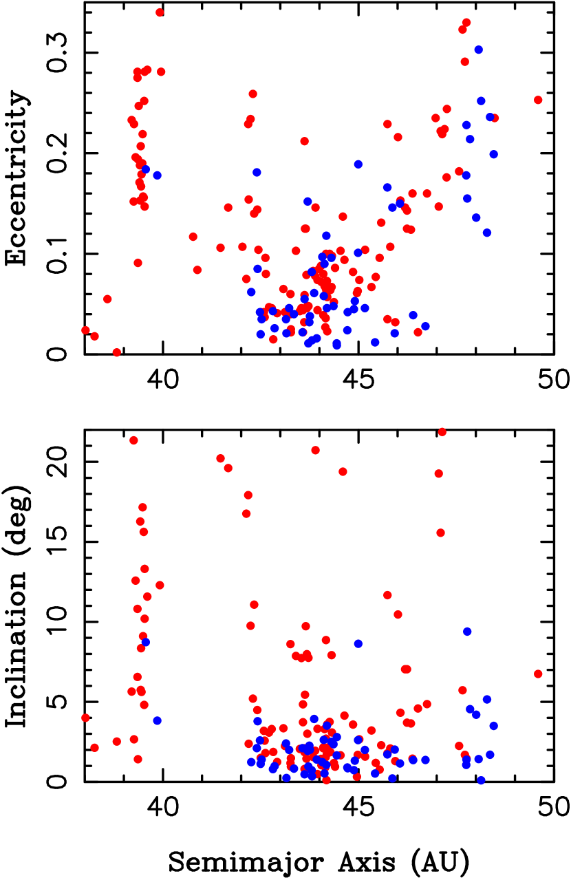
Figure 14: A comparison of the observed (red symbols) and model (blue) orbit distributions. The model distribution was obtained in the simulation with $a_{\rm N,0}=24$ AU, $\tau_{1}=30$ Myr, $a_{\rm N,1}=27.8$ AU, $\Delta a_{\rm N}=0.5$ AU, $\Delta e_{\rm N}=0.05$, and $\tau_{2}=100$ Myr. Here we assumed that the break magnitude $H_{b}$ in the original disk was 6.9 for $r\leq 45$ AU, and dropped linearly with $r$ to $H_{b}=9$ at 50 AU.

Figure 14 shows the orbital distribution obtained with $H_{\rm B}=6.9$ for $r<45$ AU, and $H_{\rm B}$ linearly increasing from $H_{\rm B}=6.9$ at $r=45$ AU to $H_{\rm B}=9$ at $r=50$ AU. The number of objects brighter than the break magnitude, $N_{\rm B}$, was kept fixed in this case. The correspondence to observations in Figure 14 is reasonable. All detected objects with low orbital eccentricities are located in the 42-47 AU region. Several bodies detected in the 2:1 resonance have $e\gtrsim 0.15$ and $i\lesssim 5^{\circ}$, just as observed. There are fewer detected bodies in the 3:2 resonance and along the $q\simeq 40$ AU line for $45<a<47.5$ AU relative to actual detections, but this can be explained if some of the actual detections are low-$i$ interlopers from the population implanted into the Kuiper belt from $r<30$ AU (Nesvorný 2015).

We tested many different combinations of the prescription for $N_{\rm B}(r)$ and $H_{\rm B}(r)$, and found that the results became unsatisfactory when the drop of $N_{\rm B}(r)$ or the rise of $H_{\rm B}(r)$ was more gradual than the ones discussed above. The underlying condition is dictated by the requirement that the disk bodies at 50 AU are either too few or too faint to be detected. Since the existing CFEPS is sensitive to $H\lesssim 8.5$ bodies on low-$i$ orbits at 50 AU, this implies that the number of bodies with $H\lesssim 8.5$ must be relatively low. A more rigorous statistical analysis of this problem is left for future work.

Another interesting possibility to consider is the original disk with a sharp edge at radius $r_{\rm edge}$ and no bodies beyond $r_{\rm edge}$. Figure 15 shows the final orbital distribution of particles that started with $r<r_{\rm edge}=44$ AU in our simulations. The transition at $\simeq$45 AU is much sharper than in Figure 4 with most bodies beyond 45 AU being located in the 2:1 resonance. These bodies started with $r<44$ AU, were captured into the 2:1 resonance, and evolved onto resonant orbits with $e\gtrsim 0.15$. Their orbital inclinations remained small. The stirred CC population with at 45-47 AU is not well reproduced in this model, but otherwise the overall distribution of bodies in Figures 5 and 15 is similar (note that no survey simulator was applied in Figure 15).

3.4 Orbital Distribution at 30-40 AU

The original disk at 30-40 AU is completely disrupted and only a small fraction of the original objects survive at the end of the simulations. Most of these survivors ended up in Neptune’s 3:2 resonance. Our initial concern with this result was that the observed 3:2 resonance population does not have a prominent low-$i$ component with physical properties that would be noticeably different from the rest. To state this differently, the bimodality of the inclination distribution and physical properties in the classical main belt does not have a counterpart among Plutinos.

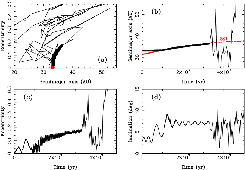
Figure 16: The orbital history of a test particle that was captured into the 3:2 resonance with Neptune, and was released from the resonance when Neptune jumped at $t=32.5$ Myr. The particle ended up on the Neptune-crossing orbit. The panels show: the (a) path of the disk particle in the $(a,e)$ projection; the red dot shows the initial orbit, (b) semimajor axis, (c) eccentricity, and (d) inclination. The 3:2 resonant angle, $\sigma_{3:2}=3\lambda-2\lambda_{\rm N}-\varpi_{\rm N}$, librates in the interval between $t\simeq 10$ Myr and $t\simeq 33$ Myr.

This issue goes back to the standard ideas about the effects of the long-range migration of Neptune on a dynamically cold disk at $>30$ AU. As Neptune migrates, the low-inclination orbits are collected in the 3:2 resonance, and should be found in the resonance today, while in fact they are not. We find that two factors contribute to mitigate this problem in our simulations. First, the population of orbits captured in the 3:2 resonance before Neptune’s jump is released from the resonance when Neptune jumps (see Figure 16 for an illustration). This reduces, by a factor of $\simeq$2-6, the number of resonant objects that remain in the 3:2 resonance at the end of our simulations (we find this by comparing the results of simulations with and without Neptune’s jump; the reduction factor positively correlates with the migration speed). Those that survive were captured after Neptune’s jump.

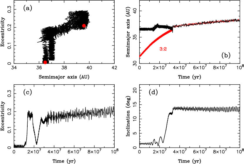
Figure 17: The orbital history of a test particle that was captured into the 3:2 resonance and remained in the resonance during the whole simulation. The orbital inclination started low and was excited to $i>10^{\circ}$ before the particle was captured into the 3:2 resonance. The panels show: the (a) path of the disk particle in the $(a,e)$ projection; the two red dots show the initial and final orbits, (b) semimajor axis, (c) eccentricity, and (d) inclination.

Second, Neptune’s migration is very slow after the jump. As the 3:2 resonance slowly sweeps through the disk, the secular resonances $\nu_{8}$ and $\nu_{18}$, located at a slightly larger semimajor axis than the 3:2 resonance, accompany this motion and excite orbits to large eccentricities and large inclinations before they could enter into the 3:2 resonance. This creates sort of a shield on outside of the migrating 3:2 resonance. Only a small fraction of bodies are seen to penetrate this shield and be captured in the resonance. Those that do have their orbital inclinations excited by the passage through $\nu_{18}$ (see Figure 17 for an example). The final inclination distribution of the resonant orbits is therefore relatively wide (see, e.g., panel (b) in Figure 4).

In the reference case discussed in Section 3.1 (with $\Delta a_{\rm N}=0.5$ AU), we find that only $\simeq$70 particles ended up on stable orbits in the 3:2 resonance, while $\simeq 650$ survived at $42<a<47$ AU. The fraction of bodies captured in the 3:2 resonance from the disk at $r>30$ AU, relative to those surviving in the main belt, is thus roughly 1/10. Other cases studied here show similar results. This implies that the population of bodies implanted in the 3:2 resonance from the disk at $r>30$ AU should be only a very small fraction of the present population of Plutinos. Indeed, existing observations indicate that the intrinsic population of Plutinos is $\sim$10 times larger than that of the CCs (e.g., Fraser et al. 2014, Adams et al. 2014). Combining the two factors of $\sim$10 discussed above, we therefore conclude that only one in $\sim$100 Plutinos should have physical characteristics similar to the CCs (red color, high albedo, binarity). This currently represents only a few objects with good orbits (the detection bias toward the low-$i$ orbits being factored in here). Future observations should be able to test this prediction.

4 Discussion

The primordial planetesimal disk between 30 and 50 AU can be divided into two parts. The inner part of the disk at 30-40 AU is disrupted during Neptune’s migration, with most of the surviving bodies being captured in the 3:2 resonance. If Neptune’s migration was relatively slow ($\tau\gtrsim 10$ Myr), as required from the inclination distribution of the HCs (Nesvorný 2015), and Neptune jumped by a fraction of AU during the instability, we estimate that only $\sim$1% of today’s Plutinos should have originated from the 30-40 AU region, while $\sim$99% were captured from the massive disk below 30 AU. The orbital inclinations of Plutinos captured from 30-40 AU are expected to be substantial, because orbits are excited by the secular resonances before they can be captured into the 3:2 resonance. Faster migration rates and/or the absence of Neptune’s jump would lead to a larger proportion of Plutinos being captured from the 30-40 AU region, and a narrower inclination distribution of the captured population. This would contradict observations, because Plutinos do not have a low-$i$ component with noticeably different physical properties.

The outer disk at 40-50 AU is somewhat excited and depleted in our simulations, but not by a large factor. The objects originally at 40-44 AU can be captured by the migrating 2:1 resonance and released at $\simeq$44 AU when Neptune jumped. The orbital characteristics of this population resemble that of the kernel, a previously unexplained feature of the Kuiper belt. This gives support to the migration model, where Neptune slowly migrates and suffers one or a few scattering encounters when at $\simeq$28 AU. As a result of the encounter(s), Neptune’s semimajor axis changes by $\simeq$0.5 AU, and then continues migrating, very slowly, toward its present value of 30.1 AU. Neptune’s 2:1 resonance, moving past 45 AU during the late stage of migration, removes $\simeq$25-70% of bodies and contributes to the orbital depletion at 45-47 AU. The effect of the 2:1 resonance cannot explain, however, on its own, the lack of low inclination orbits at $>47$ AU. Several possible solutions to this problem were discussed in Section 3.3.

The inclination excitation in the 42-47 AU region is minimal in our simulations with most bodies retaining orbits with $i<5^{\circ}$. Only a few dozens of orbits is seen to evolve to $i>5^{\circ}$. This implies that the contamination of the HCs from the cold disk at 42-47 AU should be minimal. We can roughly estimate the contamination factor from our simulations. The number of orbits with $i>5^{\circ}$ at 42-47 AU is roughly 1/20 of those surviving with $i<5^{\circ}$ at 42-47 AU. This shows that the contamination should be of the order of 5% relative to the CC population. Fraser et al. (2014) estimated that the CC population represents only $\sim$1/30 of the HC populations. Considering these two factors together, only 1 in $\sim$600 main belt objects with $i>5^{\circ}$ would be expected to have started with $i<5^{\circ}$ and $42<a<47$ AU. The real contamination factor could be larger, for example, if the disk at 42-47 AU was dynamically heated by some early process, or was excited later by the secular interactions with the fifth planet (Batygin et al. 2012; NM12).

Initially, there were 1250 particles in the 42-47 AU region in our simulations. The number of particles remaining in this region at the end of the simulations is between 550 and 700. The dynamical depletion factor is therefore only $\sim$2. Fraser et al. (2014) found that the total mass of the CCs population is $\sim 3\times 10^{-4}$ $M_{\rm Earth}$. We can therefore estimate that the original mass in the 42-47 AU region was $\sim 6\times 10^{-4}$ $M_{\rm Earth}$, most of which was probably concentrated below $\simeq$45 AU (see the discussion in Section 3.3). This roughly implies $\sim 2\times 10^{-4}$ $M_{\rm Earth}$ in each radial AU, or the surface density of solids $\Sigma_{\rm s}\sim 2\times 10^{-5}$ g cm^-2. This is $\sim$4 orders of magnitude smaller than the surface density needed to form sizable objects in the standard coagulation model (Kenyon et al. 2008). It is possible that the original surface density was much higher and bodies were removed by fragmentation during collisions (Pan & Sari 2005), but the presence of loosely bound binaries places a strong constraint on how much mass can be removed (Nesvorný et al. 2011).

A possible solution of this problem is that the CCs formed by a gravitational collapse of solids that were locally concentrated by their interaction with the gaseous nebula. For example, Youdin & Goodman (2005) suggested that large planetesimals can form from the concentrations of particles produced by the streaming instability. Numerical simulations give support to this model and show that the streaming instability can operate in a low-mass environment assuming that the local metalicity can be slightly increased over the solar metalicity (Johansen et al. 2009). Since only a small fraction of the available mass may be converted into sizable planetesimals by this process, the original surface density in the 42-47 AU region could have been higher than inferred above. The large binary fraction among the CCs ($>$30%; Noll et al. 2007, 2014) can provide an evidence for the gravitational collapse model, because binaries are expected to form if the collapsing clouds have important rotation (Nesvorný et al. 2010).

Figure 4: The final distribution of orbits obtained in the simulation with $a_{\rm N,0}=24$ AU, $\tau_{1}=30$ Myr, $a_{\rm N,1}=27.8$ AU, $\Delta a_{\rm N}=0.5$ AU, $\Delta e_{\rm N}=0.05$, and $\tau_{2}=100$ Myr. At the beginning of the simulation, 5000 test particles were distributed on low-inclination ($\sigma_{i}=2^{\circ}$) low-eccentricity ($\sigma_{e}=0.01$) orbits between 30 and 50 AU. The bold symbols denote the orbits that ended with $40<a<47$ AU and $q=a(1-e)>36$ AU.

Figure 5: The same as Figure 1 but without labeling of different populations. This figure is useful when comparing the simulation results with observations.

Figure 6: The semimajor axis distribution of the model (solid and dot-dashed lines) and observed (dashed) KBOs. The observed orbits were taken from Figure 1. The model orbits were obtained in a simulation with $a_{\rm N,0}=24$ AU, $\tau_{1}=30$ Myr, $a_{\rm N,1}=27.8$ AU, $\Delta e_{\rm N}=0.05$, $\tau_{2}=100$ Myr, and $\sigma_{e}=0.01$. Here we highlight the difference between cases with $\Delta a_{\rm N}=0.5$ AU (solid line) and $\Delta a_{\rm N}=0$ (dot-dashed line). The case with $\Delta a_{\rm N}=0$ shows the orbit density increasing with the semimajor axis. It does not fit observations well. The case with $\Delta a=0.5$ AU, on the other hand, shows a concentration of orbits at the location of the Kuiper belt kernel at 44 AU. These orbits were left behind by the 2:1 resonance when Neptune jumped. In both cases, we only consider orbits with $i<5^{\circ}$ and $q=a(1-e)>36$ AU.

Figure 9: The final distribution of orbits obtained in the simulation with $a_{\rm N,0}=24$ AU, $\tau_{1}=30$ Myr, $a_{\rm N,1}=27.8$ AU, $\Delta e_{\rm N}=0.1$, and $\tau_{2}=100$ Myr. The panels on the left show the result for $\Delta a_{\rm N}=0$, while those on the right show the result for $\Delta a_{\rm N}=0.5$ AU. The concentration of orbits at $\simeq$44 AU in the right panels was created by the 2:1 resonance when Neptune jumped. At the beginning of the simulation, 5000 test particles were distributed on low-inclination ($\sigma_{i}=2^{\circ}$) low-eccentricity ($\sigma_{e}=0.01$) orbits between 30 and 50 AU. The bold symbols denote the orbits that ended with $40<a<47$ AU and $q=a(1-e)>36$ AU.

Figure 10: The final distribution of orbits obtained in the simulation with $a_{\rm N,0}=24$ AU, $\tau_{1}=30$ Myr, $a_{\rm N,1}=27.8$ AU, $\Delta e_{\rm N}=0.1$, and $\tau_{2}=100$ Myr. The panels on the left show the result for $\Delta a_{\rm N}=0.25$ AU, while those on the right show the result for $\Delta a_{\rm N}=0.75$ AU. The concentration of orbits at $\simeq$44 AU in the right panels was created by the 2:1 resonance when Neptune jumped. The bold symbols denote the orbits that ended with $40<a<47$ AU and $q=a(1-e)>36$ AU.

Figure 11: The final distribution of orbits obtained in the simulation with $a_{\rm N,0}=24$ AU, $\tau_{1}=10$ Myr, $a_{\rm N,1}=27.8$ AU, $\Delta e_{\rm N}=0.1$, and $\tau_{2}=30$ Myr. The panels on the left show the result for $\Delta a_{\rm N}=0$, while those on the right show the result for $\Delta a_{\rm N}=0.5$ AU. The bold symbols denote the orbits that ended with $40<a<47$ AU and $q=a(1-e)>36$ AU.

Figure 12: The same as Figure 9 but for the test particles having larger initial eccentricities ($\sigma_{e}=0.05$).

Figure 13: The semimajor axis distribution of the model (solid line) and observed (dashed) bodies. The model orbits were obtained with $a_{\rm N,0}=24$ AU, $\tau_{1}=30$ Myr, $a_{\rm N,1}=27.8$ AU, $\Delta a_{\rm N}=0.5$ AU, $\Delta e_{\rm N}=0.05$, and $\tau_{2}=100$ Myr. The CFEPS simulator was applied here. We assumed that the number density of objects with $H<9$ per semimajor axis interval was constant up to 45 AU, and dropped linearly from 45 AU to zero at 50 AU.

Figure 15: The final distribution of orbits obtained in the simulation with $a_{\rm N,0}=24$ AU, $\tau_{1}=30$ Myr, $a_{\rm N,1}=27.8$ AU, $\Delta a_{\rm N}=0.5$ AU, $\Delta e_{\rm N}=0.05$, and $\tau_{2}=100$ Myr. Here we assumed that the initial disk had an outer edge at 44 AU, and there were no bodies initially located beyond 44 AU.

References

- Adams et al. (2014) Adams, E. R., Gulbis, A. A. S., Elliot, J. L., et al. 2014, AJ, 148, 55
- Batygin et al. (2011) Batygin, K., Brown, M. E., & Fraser, W. C. 2011, ApJ, 738, 13
- Batygin et al. (2012) Batygin, K., Brown, M. E., & Betts, H. 2012, ApJ, 744, L3
- Bernstein et al. (2004) Bernstein, G. M., Trilling, D. E., Allen, R. L., et al. 2004, AJ, 128, 1364
- Brown (2001) Brown, M. E. 2001, AJ, 121, 2804
- Chiang & Jordan (2002) Chiang, E. I., & Jordan, A. B. 2002, AJ, 124, 3430
- Chiang et al. (2003) Chiang, E. I., Jordan, A. B., Millis, R. L., et al. 2003, AJ, 126, 430
- Dawson & Murray-Clay (2012) Dawson, R. I., & Murray-Clay, R. 2012, ApJ, 750, 43
- Duncan et al. (1995) Duncan, M. J., Levison, H. F., & Budd, S. M. 1995, AJ, 110, 3073
- Fraser et al. (2014) Fraser, W. C., Brown, M. E., Morbidelli, A., Parker, A., & Batygin, K. 2014, ApJ, 782, 100
- Gladman et al. (2008) Gladman, B., Marsden, B. G., & Vanlaerhoven, C. 2008, The Solar System Beyond Neptune, 43
- Gomes (2003) Gomes, R. S. 2003, Icarus, 161, 404
- Gulbis et al. (2010) Gulbis, A. A. S., Elliot, J. L., Adams, E. R., et al. 2010, AJ, 140, 350
- Hahn & Malhotra (1999) Hahn, J. M., & Malhotra, R. 1999, AJ, 117, 3041
- Hahn & Malhotra (2005) Hahn, J. M., & Malhotra, R. 2005, AJ, 130, 2392
- Jewitt et al. (1996) Jewitt, D., Luu, J., & Chen, J. 1996, AJ, 112, 1225
- Johansen et al. (2009) Johansen, A., Youdin, A., & Mac Low, M.-M. 2009, ApJ, 704, L75
- Kavelaars et al. (2008) Kavelaars, J., Jones, L., Gladman, B., Parker, J. W., & Petit, J.-M. 2008, The Solar System Beyond Neptune, 59
- Kavelaars et al. (2009) Kavelaars, J. J., Jones, R. L., Gladman, B. J., et al. 2009, AJ, 137, 4917
- Kenyon et al. (2008) Kenyon, S. J., Bromley, B. C., O’Brien, D. P., & Davis, D. R. 2008, The Solar System Beyond Neptune, 293
- Knezevic et al. (1991) Kněžević, Z., Milani, A., Farinella, P., Froeschlé, C., & Froeschlé, C. 1991, Icarus, 93, 316
- Levison & Duncan (1994) Levison, H. F., & Duncan, M. J. 1994, Icarus, 108, 18
- Levison & Morbidelli (2003) Levison, H. F., & Morbidelli, A. 2003, Nature, 426, 419
- Levison et al. (2008) Levison, H. F., Morbidelli, A., Vanlaerhoven, C., Gomes, R., & Tsiganis, K. 2008, Icarus, 196, 258
- Malhotra (1993) Malhotra, R. 1993, Nature, 365, 819
- Malhotra (1995) Malhotra, R. 1995, AJ, 110, 420
- Marcus et al. (2011) Marcus, R. A., Ragozzine, D., Murray-Clay, R. A., & Holman, M. J. 2011, ApJ, 733, 40
- Morbidelli et al. (2007) Morbidelli, A., Tsiganis, K., Crida, A., Levison, H. F., & Gomes, R. 2007, AJ, 134, 1790
- Morbidelli et al. (2008) Morbidelli, A., Levison, H. F., & Gomes, R. 2008, The Solar System Beyond Neptune, 275
- Morbidelli et al. (2014) Morbidelli, A., Gaspar, H. S., & Nesvorny, D. 2014, Icarus, 232, 81
- Murray-Clay & Chiang (2005) Murray-Clay, R. A., & Chiang, E. I. 2005, ApJ, 619, 623
- Murray-Clay & Chiang (2006) Murray-Clay, R. A., & Chiang, E. I. 2006, ApJ, 651, 1194
- Nesvorný et al. (2015) Nesvorný, D. 2015., AJ, in press
- Nesvorný & Morbidelli (2012) Nesvorný, D., & Morbidelli, A. 2012 (NM12), AJ, 144, 117
- Nesvorný et al. (2010) Nesvorný, D., Youdin, A. N., & Richardson, D. C. 2010, AJ, 140, 785
- Nesvorný et al. (2011) Nesvorný, D., Vokrouhlický, D., Bottke, W. F., Noll, K., & Levison, H. F. 2011, AJ, 141, 159
- Nesvorný et al. (2015) Nesvorný, D, Brož, M., Carruba, V. 2015, In Asteroids IV, Arizona University Press.
- Noll et al. (2008) Noll, K. S., Grundy, W. M., Chiang, E. I., Margot, J.-L., & Kern, S. D. 2008, The Solar System Beyond Neptune, 345
- Noll et al. (2014) Noll, K. S., Parker, A. H., & Grundy, W. M. 2014, AAS/Division for Planetary Sciences Meeting Abstracts, 46, #507.05
- Pan & Sari (2005) Pan, M., & Sari, R. 2005, Icarus, 173, 342
- Petit et al. (2011) Petit, J.-M., Kavelaars, J. J., Gladman, B. J., et al. 2011, AJ, 142, 131
- Sheppard et al. (2012) Sheppard, S. S., Ragozzine, D., & Trujillo, C. 2012, AJ, 143, 58
- Thommes et al. (1999) Thommes, E. W., Duncan, M. J., & Levison, H. F. 1999, Nature, 402, 635
- Tsiganis et al. (2005) Tsiganis, K., Gomes, R., Morbidelli, A., & Levison, H. F. 2005, Nature, 435, 459
- Tsiganis et al. (2005) Vokrouhlický, D., & Nesvorný, D. 2015, AJ, submitted
- Wolff et al. (2012) Wolff, S., Dawson, R. I., & Murray-Clay, R. A. 2012, ApJ, 746, 171
- Youdin & Goodman (2005) Youdin, A. N., & Goodman, J. 2005, ApJ, 620, 459