Enhanced Lasso Recovery on Graph

Abstract

This work aims at recovering signals that are sparse on graphs. Compressed sensing offers techniques for signal recovery from a few linear measurements and graph Fourier analysis provides a signal representation on graph. In this paper, we leverage these two frameworks to introduce a new Lasso recovery algorithm on graphs. More precisely, we present a non-convex, non-smooth algorithm that outperforms the standard convex Lasso technique. We carry out numerical experiments on three benchmark graph datasets.

1 Sparse Representation on Graphs

The goal of this work is to reconstruct signals on graphs that are supposed to be sparse in the graph Fourier representation. In this context, we will deal here with two main concepts, graph and sparsity, which have gathered a lot of attention in the recent years with the emergence of Compressed Sensing and Big Data. Let us introduce briefly these two concepts in the rest of this section.

Graph/network is a powerful tool to represent complex high-dimensional datasets, in the sense that a graph structures data with respect to their similarities. Graphs have become increasingly more considered in applications such as search engines, social networks, airline routes, 3D geometric shapes, human brain connectivity, etc. Mathematics offer strong theoretical tools to analyze graphs with Harmonic Analysis and Spectral Graph Theory. An essential graph analysis tool is the graph Laplacian operator, which is the discrete approximation of the continuum Laplace-Beltrami operator for smooth manifolds. It is known that the eigenvectors of the Laplace-Beltrami operator provide a local parametrization of the manifold [1]. Equivalently, the eigenvectors of the graph Laplacian, also called graph Fourier modes, provides a representation of the graph. Given a graph with $(V,E,W)$, $V$, $E$ and $W$ being respectively the set of $n$ nodes, the set of edges and the similarity/adjacency matrix, then the (unnormalized) graph Laplacian operator is defined as

$$L=D-W,$$

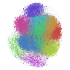
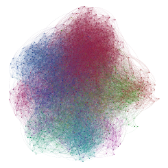
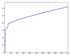
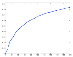
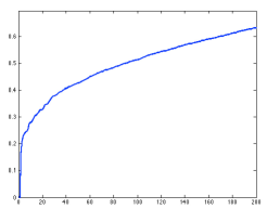
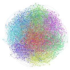
where $D$ is the diagonal degree matrix s.t. $D_{ii}=\sum_{j}W_{ij}$. $L$ is symmetric and positive-semidefinite, i.e. its eigenvalues $\lambda_{i},\forall i$ are nonnegative. The graph Fourier modes are given by the eigenvectors $\{u_{i}\}_{i=1}^{n}$ of $L$ and can be represented by the orthogonal matrix $U=(u_{1},...,u_{n})\in\mathbb{R}^{n\times n}$ s.t. $U^{\star}U=I$. The graph Fourier basis $U$ acts as a basis to represent, analyze and process signals on graph. For example, one can represent a function $f:V\rightarrow\mathbb{R}$ on graph as $f(i)=\sum_{l=1}^{n}\hat{f}_{l}\cdot u_{l}(i)$ where $\hat{f}_{l}=\langle f,u_{l}\rangle=\sum_{i=1}^{n}f(i)\cdot u_{l}(i)$ is its Fourier transform. In this paper, we consider three well-known graphs. First, the synthetic LFR graph, which was introduced in [2] to study community graphs. Here, the number of nodes is chosen to be $n=1,000$, the number of communities is $10$ and the degree of community overlapping is $\mu=0.4$. Second, we consider a coarse version (for computational speedup) of the benchmark MNIST dataset of NYU [3] with $n=1,176$ nodes and the number of classes is $10$. Last, we use a coarse version of the well-known 20newsgroups dataset of CMU [4] with $n=1,432$ nodes and the number of classes is $20$. All three dataset graphs are illustrated on Figure 1 with their graph Laplacian spectrum.

(a) LFR

(b) MNIST

(c) 20NEWS

(d) LFR

(e) MNIST

(f) 20NEWS

Figure 1: Graph and spectrum of LFR, MNIST, 20NEWS.

Sparse recovery is currently one of the most studied topics in signal processing. The main goal is to reconstruct signals that are supposed to be sparse in some basis representation. For example, in medical imaging, one of the objectives of sparsity is to speed up MRI acquisition by reconstructing an image in the Fourier basis given a small number of Fourier samples. This problem can be generalized to find the solution of a underestimated linear system of equations, which is generally ill-posed, with the constraint that the solution is sparse. Finding the solution of this problem is however impracticable because it is a NP-hard combinatorial problem. But Candes, Romberg, Tao and Donoho showed in [5, 6] that using an $\ell_{1}$ relaxation and under some conditions on the linear operator, known as the Restricted Isometry Property (RIP), and the measurements, known as incoherence property, there exists a tight convex relaxation of the NP-hard problem, that is easily tractable. However, it has recently been observed that the $\ell_{1}$ relaxation technique can be improved with reweighed $\ell_{1}$ [7], $\ell_{p},p<1$ [8], difference of convex functions $\ell_{1}$-$\ell_{2}$ [9] and smoothed $\ell_{1}/\ell_{2}$ ratio[10]. These recent works suggest that non-convex relaxations may outperform the original $\ell_{1}$ sparse recovery. In this work, we follow this line of research and we introduce a new non-convex algorithm for sparse recovery on graph. Specifically, our goal is to improve Lasso problems on graph.

2 Enhanced Sparsity

Starting from the standard $\ell_{1}$ problem for sparse recovery

$$\min_{x}\|x\|_{1}\quad\textrm{ s.t. }\quad Ux=f_{0},$$

where $x$ is a sparse signal to be recovered, $U$ is the graph Fourier basis, and $f_{0}$ are the given measurements, we propose the following enhanced recovery model

$$\min_{x}\|x\|_{1}\quad\textrm{ s.t. }\quad Ux=f_{0},\quad\|x\|_{2}=1.$$

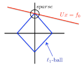
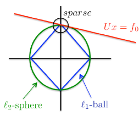
The new additional constraint, i.e. the $\ell_{2}$ unit sphere, is a non-convex set that is here essential for enhancing sparse recovery. Basically, it forces the solution to be at the intersection of the $\ell_{1}$-ball and the $\ell_{2}$-sphere, which are precisely the locations of sparse points in the Euclidean domain, see Figure 2. Observe now that the new constrained $\ell_{1}$ optimization problem is equivalent to

$$\min_{x}\frac{\|x\|_{1}}{\|x\|_{2}}\quad\textrm{ s.t. }\quad Ux=f_{0}$$ (1)

The equivalence comes from the fact that the ratio $\ell_{1}/\ell_{2}$ is a zero-homogenous function, i.e. $F(\alpha x)=F(x),\alpha>0$. This means that the solution $x^{\star}$ is the same as $\alpha x^{\star}$, $\forall\alpha$. Particularly, for the specific value of $\alpha$ such that $x^{\star}$ belongs to the unit sphere $\|x^{\star}\|_{2}=1$. Figure 2 compares geometrically the standard $\ell_{1}$ and the new ratio model $\ell_{1}/\ell_{2}$. At a first glance, both models promote sparsity and the new model does not appear to bring anything new but a more complex problem. However, this figure acts as a simple illustration and one must remember that the recovery performance depends also on the incoherence property about the number of observed measurements. In this context, the major motivation to go beyond convexity with the recent works [7, 8, 9] is to precisely improve sparse recovery with a smaller number of measurements than the standard approach. We will see that the newly proposed model holds this property.

(a) $\ell_{1}$

(b) $\ell_{1}/\ell_{2}$

Figure 2: Standard $\ell_{1}$ and $\ell_{1}/\ell_{2}$.

3 Optimization

We consider a different version of (1) that is robust to noise:

$$\min_{x}\frac{\|x\|_{1}}{\|x\|_{2}}+\frac{\lambda}{2}\|Ux-f_{0}\|_{2}^{2}$$ (2)

Problem (2) is a non-smooth and non-convex optimization problem. The $\ell_{1}$/non-smooth part of the problem can be handled quite efficiently with techniques introduced in Compressed Sensing such as Alternating Direction Method of Multipliers (ADMM) [11] or Uzawa-type Primal-Dual technique [12]. However, the non-convex part is more challenging. For general non-convex problems, it is difficult to design an algorithm that is fast, accurate, robust and also guaranteed to converge, or at least that satisfies the monotonicity property. Monotonicity means that the energy is guaranteed to decrease at each iteration, although the problem is non-convex. In this situation, most non-convex algorithms only find solutions that are critical points or local minimizers, and rarely global minimizers.

3.1 Proximal Forward-Backard Splitting Algorithm

We develop in this section an algorithm for the ratio optimization problem (2). A related numerical scheme was introduced in [13] in the different context of data clustering. Let $T(x)=\|x\|_{1}$, $B(x)=\|x\|_{2}$, $E(x)=T(x)/B(x)$ and $F(x)=\frac{\lambda}{2}\|Ux-f_{0}\|_{2}^{2}$ such that we want to solve

$$\min_{x}\frac{T(x)}{B(x)}+F(x).$$

Let us consider a semi-implicit gradient flow for this problem:

$$\frac{x^{k+1}-x^{k}}{\tau^{k}} = -\frac{\partial T(x^{k+1})\cdot B(x^{k})-T(x^{k})\cdot\partial B(x^{k})}{B^{2}(x^{k})}-\partial F(x^{k+1}),$$

where $\partial$ stands for the subdifferentials of $T$ and $B$ (which is not unique for $\ell_{1}$ but is for $\ell_{2}$) and $\tau^{k}$ is the time step. This provides the optimality condition

$$x^{k+1}-(x^{k}+\tau^{k}\frac{E^{k}}{B^{k}}\partial B(x^{k}))+\frac{\tau^{k}}{B^{k}}\partial T^{k+1}+\tau^{k}\partial F^{k+1}\ni 0,$$ (3)

where the notations $T^{k}=T(x^{k})$ and $B^{k}=B(x^{k})$ are used. This leads to a two-step iterative scheme:

$$(1)\quad y^{k}=x^{k}+c_{0}^{k}\partial B(x^{k})$$

and

$$(2)\quad x^{k+1} = \arg\min_{x}c_{1}^{k}T(x)+\frac{\tau^{k}}{2}F(x)+\frac{1}{2}\|x-y^{k}\|_{2}^{2}$$

$$= \textrm{prox}_{c_{1}^{k}T+\frac{\tau^{k}}{2}F}(y^{k}),$$

where $c_{0}^{k}=\tau^{k}E^{k}/B^{k}$ and $c_{1}^{k}=\tau^{k}/B^{k}$. The second step is the proximal operator [12, 14] of the convex function $c_{1}^{k}T+\frac{\tau^{k}}{2}F$. Overall, we have designed a proximal forward-backward splitting algorithm to solve (2) as the solution is given by

$$x^{k+1}=\textrm{prox}_{c_{1}^{k}T+\frac{\tau^{k}}{2}F}(x^{k}+c_{0}^{k}\partial B(x^{k})).$$ (4)

In the next section, we will show that the proposed iterative algorithm is (almost) monotonic, i.e. its energy is guaranteed to decrease at each iteration.

3.2 Monotonicity

We show the following quasi-monotonicity result:

$$\frac{B^{k+1}}{B^{k}}(E^{k}-E^{k+1})+(F^{k}-F^{k+1})\geq\frac{\|x^{k}-x^{k+1}\|_{2}^{2}}{\tau^{k}}$$ (5)

Proof. Define the convex functions

$$\mathcal{G}^{k}(x) = c_{0}^{k}B(x)+\tau^{k}F(x),$$ (6)

$$\mathcal{F}^{k}(x) = c_{1}^{k}T(x)+\tau^{k}F^{k},$$ (7)

and observe that $\mathcal{G}^{k}(x^{k})=\mathcal{F}^{k}(x^{k})$ for latter use. We remind the general definition of the subdifferential $\partial\mathcal{E}$ of a convex function $\mathcal{E}$:

$$\mathcal{E}(x_{1})\geq\mathcal{E}(x_{2})+\langle x_{1}-x_{2},y_{2}\rangle,\ \forall y_{2}\in\partial\mathcal{E}(x_{2}).$$ (8)

We plug $x_{1}=x^{k+1}$, $x_{2}=x^{k}$ and $\mathcal{E}=\mathcal{G}$ in (8):

$$\mathcal{G}^{k}(x^{k+1})\geq\mathcal{G}^{k}(x^{k})+\langle x^{k+1}-x^{k},\partial\mathcal{G}^{k}(x^{k})\rangle$$ (9)

If we now observe that the first step of the algorithm is $y^{k}=x^{k}+v^{k}$ with $v^{k}=c_{0}^{k}\partial B(x^{k})=\partial\mathcal{G}^{k}(x^{k})$ then (9) becomes

$$\mathcal{G}^{k}(x^{k+1})\geq\mathcal{G}^{k}(x^{k})+\langle x^{k+1}-x^{k},v^{k}\rangle.$$ (10)

Let us now plug $x_{1}=x^{k}$, $x_{2}=x^{k+1}$ and $\mathcal{E}=\mathcal{F}$ in (8):

$$\mathcal{F}^{k}(x^{k})\geq\mathcal{F}^{k}(x^{k+1})+\langle x^{k}-x^{k+1},\partial\mathcal{F}^{k}(x^{k+1})\rangle.$$ (11)

Notice that the optimality condition (3) reads $x^{k+1}-y^{k}+\partial\mathcal{F}^{k}(x^{k+1})\ni 0$ and thus $y^{k}-x^{k+1}\in\partial\mathcal{F}^{k}(x^{k+1})$. This implies that (11) may be written as

$$\mathcal{F}^{k}(x^{k}) \geq \mathcal{F}^{k}(x^{k+1})+\langle x^{k}-x^{k+1},y^{k}-x^{k+1}\rangle$$ (12)

$$\geq \mathcal{F}^{k}(x^{k+1})+\|x^{k}-x^{k+1}\|_{2}^{2}+\langle x^{k}-x^{k+1},v^{k}\rangle$$

Adding (10) and (12) and using the fact that $\mathcal{G}^{k}(x^{k})=\mathcal{F}^{k}(x^{k})$ we have

$$\mathcal{G}^{k}(x^{k+1})\geq\mathcal{F}^{k}(x^{k+1})+\|x^{k}-x^{k+1}\|_{2}^{2}$$ (13)

Using the definition (6) and (7), this inequality can be rewritten as (5), which is the desired result. $\Box$

Notes. Observe that close to the steady-state solution, we have $B^{k+1}/B^{k}\rightarrow 1$ for $k\rightarrow\infty$ and the quasi-monotonicity tends to a monotonicity property. Second, see that if we had access to the quantity $B^{k+1}$ (or a good estimation) then we would set $\tau^{k}=\frac{B^{k}}{B^{k+1}}\tau_{0}$ and this would imply

$$E_{Tot}^{k}-E_{Tot}^{k+1}\geq\|x^{k}-x^{k+1}\|_{2}^{2}/\tau^{k},$$

where $E_{Tot}=E+F$, and thus unconditional monotonicity for any $\tau_{0}$.

4 Applications

4.1 Enhanced Lasso on Graphs

The Algorithm. The standard Lasso problem on graph is $\min_{x}\|x\|_{1}+\frac{\lambda}{2}\|Ux-f_{0}\|_{2}^{2}$ where $U$ is the sensing matrix, here the graph Fourier modes. Function $f_{0}$ is the signal measured on the graph. It is generated as $f_{0}=U(x_{0}+n)$ where $x_{0}$ is a pure sparse signal with 5% of non-zero entries uniformly chosen between $[-1,1]$ and $n$ is the noise, a Gaussian distribution with standard deviation $\sigma=0.1$. The goal is to recover the sparse signal $x_{0}$. We recall that the proposed enhanced Lasso problem on graph is $\min_{x}\frac{\|x\|_{1}}{\|x\|_{2}}+\frac{\lambda}{2}\|Ux-f_{0}\|_{2}^{2}$. We use the proximal forward-backward splitting algorithm introduced in Section 3.1 to solve it. That is, Step 1: $y^{k}=x^{k}+\frac{\tau^{k}E^{k}}{B^{k}}\partial\|x\|_{2}|_{x^{k}}=x^{k}+\frac{\tau^{k}E^{k}}{B^{k}}\frac{x^{k}}{\|x^{k}\|_{2}}$, and Step 2: $x^{k+1}=\arg\min_{x}F(x)+G(x)$ where $F(x)=\|x\|_{1}$ and $G(x)=\frac{E^{k}\lambda}{2}\|Ux-f_{0}\|_{2}^{2}+\frac{E^{k}}{2\tau^{k}}\|x-y^{k}\|_{2}^{2}$. We may write this problem as a saddle-point problem $\min_{x}\max_{p}\langle p,x\rangle-F^{\star}(p)+G(x)$ where $F^{\star}$ is the barrier function of the $\ell_{\infty}$ unit ball such that

$$F^{\star}(p)=\left\{\begin{array}[]{ll}0&\textrm{ if }|p|\leq 1,\\ +\infty&\textrm{ otherwise, }\end{array}\right.$$ (16)

Note that $G(x)$ is uniformly convex so that we can apply the accelerated primal-dual algorithm of [14]. The algorithm consists in iterating the following steps:

$$p^{n+1} = \textrm{prox}_{\sigma^{n}F^{\star}}(p^{n}+\sigma^{n}\bar{x}^{n})$$ (17)

$$x^{n+1} = \textrm{prox}_{\eta^{n}G}(x^{n}-\eta^{n}p^{n+1})$$ (18)

$$\theta^{n+1} = 1/\sqrt{1+2\gamma\eta^{n}},\tau^{n+1}=\theta^{n+1}\eta^{n},\sigma^{n+1}=\sigma^{n}/\theta^{n+1}$$ (19)

$$\bar{x}^{n+1} = x^{n+1}+\theta^{n+1}(x^{n+1}-x^{n})$$ (20)

The scheme converges quickly, with order $O(1/n^{2})$, provided that $\sigma^{0}=\eta^{0}=1$. The first inner proximal problem has an analytical solution

$$\textrm{prox}_{\sigma^{n}F^{\star}}(z)=z/\max\{1,|z|\},$$

and the second inner proximal problem has also a closed-form solution

$$\textrm{prox}_{\eta^{n}G}(z)=\frac{z+E^{k}\lambda\eta^{n}U^{*}f_{0}+E^{k}\eta^{n}y^{k}/\tau^{k}}{1+E^{k}\lambda\eta^{n}+E^{k}\eta^{n}/\tau^{k}}.$$

As the two proximal operators are fast to solve, so it is for the general algorithm. In fact, solving the non-convex ratio problem (2) for sparse recovery can be seen as solving the standard Lasso problem with the addition of a convex quadratic term $\|x-y^{k}\|_{2}^{2}$ and updating $y^{k}$ each time the monotonicity condition (5) is satisfied. We summarize the algorithm here.

Algorithm. Initialize $x^{0}=U^{*}f_{0}$, $\sigma^{n=0}=\eta^{n=0}=1$, $\gamma=1$, and iterate $k$ until convergence
(1) $\tau^{k}=B^{k}$
(2) $y^{k}=x^{k}+E^{k}\frac{x^{k}}{\|x^{k}\|_{2}}$
(3) Inner loop: iterate $n$ until the monotonicity condition, $B^{n}/B^{k}(E^{k}-E^{n})+(F^{k}-F^{n})\geq\|x^{k}-x^{n}\|_{2}^{2}/\tau^{k}$, is satisfied:
(3i) $p^{n+1}=(p^{n}+\sigma^{n}\bar{x}^{n})/\max\{1,|p^{n}+\sigma^{n}\bar{x}^{n}|\}$
(3ii) $x^{n+1}=\frac{x^{n}-\eta^{n}p^{n+1}+E^{k}\lambda\eta^{n}U^{*}f_{0}+E^{k}\eta^{n}y^{k}/\tau^{k}}{1+E^{k}\lambda\eta^{n}+E^{k}\eta^{n}/\tau^{k}}$
(3iii) $\theta^{n+1}=1/\sqrt{1+2\gamma\eta^{n}},\tau^{n+1}=\theta^{n+1}\eta^{n},\sigma^{n+1}=\sigma^{n}/\theta^{n+1}$
(3iv) $\bar{x}^{n+1}=x^{n+1}+\theta^{n+1}(x^{n+1}-x^{n})$
(4) $x^{k}=x^{n+1}$
Note: the time step $\tau^{k}=B^{k}$ was chosen experimentally, and is the subject of future study.

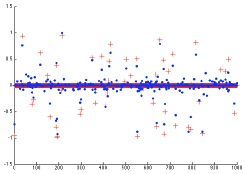
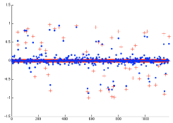
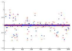
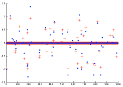
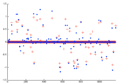
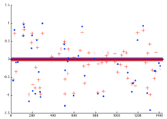
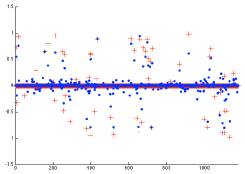
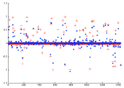
Numerical Experiments. We compare standard Lasso and enhanced Lasso on graphs. We test on the LFR, MNIST and 20NEWS graphs. The value of the parameter $\lambda$ that balances the sparsity term and the fidelity term is chosen to minimize the recovery error defined as $\|x-x_{0}\|_{2}/\|x\|_{2}$ for all models and all graphs. The results are reported on Table 1 and Figure 3. Overall, the proposed enhanced Lasso model performs better than the standard one, but it is 2-3 times slower.

	Standard Lasso	Proposed Lasso
LFR	0.419	0.309
MNIST	0.417	0.302
20NEWS	0.481	0.325

Table 1: Accuracy for standard Lasso vs proposed Lasso on three graphs.

(a) LFR, $\ell_{1}$

(b) MNIST, $\ell_{1}$

(c) 20NEWS, $\ell_{1}$

(d) LFR, $\ell_{1}/\ell_{2}$

(e) MNIST, $\ell_{1}/\ell_{2}$

(f) 20NEWS, $\ell_{1}/\ell_{2}$

Figure 3: Standard Lasso vs Proposed Lasso on three graphs.

4.2 Enhanced Lasso-Inpaiting on Graphs

The Algorithm. In this section, we add a layer of difficulty by removing a set of observed measurements in $f_{0}$. In other words, we do not observe the whole function $f_{0}$ but only a portion of it. This problem is equivalent to a Lasso-Inpainting problem. For this, a diagonal selector matrix $R$ is added to the linear operator $U$ such that

$$R_{ii}=\left\{\begin{array}[]{ll}1&\textrm{ if }i\in\Omega_{obs},\\ 0&\textrm{ otherwise, }\end{array}\right.$$ (23)

$\Omega_{obs}$ being the set of observed measurements, and $R_{ii}=0$ otherwise. The formulation is thus $\min_{x}\|x\|_{1}+\frac{\lambda}{2}\|RUx-f_{0}\|_{2}^{2}$. The enhanced Lasso-Inpainting is naturally

$$\min_{x}\frac{\|x\|_{1}}{\|x\|_{2}}+\frac{\lambda}{2}\|RUx-f_{0}\|_{2}^{2}.$$

We apply the same technique as in Section 4.1 to compute a solution to the problem. The only change is the solution of the inner proximal problem $\textrm{prox}_{\eta^{n}G}(z)=U^{*}(Ub/K)$ where $b=z+E^{k}\lambda\eta^{n}RU^{*}f_{0}+E^{k}\eta^{n}y^{k}/\tau^{k}$ and $K=I+E^{k}\lambda\eta^{n}R+E^{k}\eta^{n}/\tau^{k}$, which is also fast to compute.

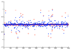
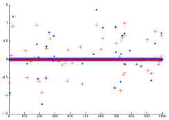
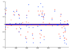
Numerical Experiments. We compare standard Lasso-Inpainting and enhanced Lasso-Inpainting on graphs. We test on the LFR, MNIST and 20NEWS graphs. We remove 40% of measurements of $f_{0}$ with $R$. The value of the parameter $\lambda$ is again chosen to minimize the recovery error defined as $\|x-x_{0}\|_{2}/\|x\|_{2}$ for all models and all graphs. The results are reported on Table 2 and Figure 4. Overall, the proposed enhanced Lasso-Inpainting model also performs better than the standard one, but it is 2-3 times slower.

	Standard Lasso-Inp	Proposed Lasso-Inp
LFR	0.667	0.540
MNIST	0.509	0.362
20NEWS	0.516	0.468

Table 2: Accuracy for standard Lasso-Inpainting vs proposed Lasso-Inpainting on three graphs.

(a) LFR, $\ell_{1}$

(b) MNIST, $\ell_{1}$

(c) 20NEWS, $\ell_{1}$

(d) LFR, $\ell_{1}/\ell_{2}$

(e) MNIST, $\ell_{1}/\ell_{2}$

(f) 20NEWS, $\ell_{1}/\ell_{2}$

Figure 4: Standard Lasso-Inpainting vs Proposed Lasso-Inpainting on three graphs.

5 Conclusion

A new sparse recovery algorithm for Lasso-type problems on graph has been introduced. Numerical experiments have shown improvements over the standard $\ell_{1}$ algorithms. This result leverages the recent idea to go beyond $\ell_{1}$ convexity and explore non-convex, non-smooth techniques to find better sparse solutions. In this context, the closest works to ours are (i) the difference of convex (DC) functions [9] and (ii) the smoothed $\ell_{1}/\ell_{2}$ technique [10]. We would like to explore in a future work the relationship between our model and these models. Particularly, a direct application of Dinkelbach technique [15] reveals that minimizing the ratio is equivalent to minimize the DC model $\ell_{1}-\alpha\ell_{2}$ with $\alpha$ being the minimum value of the ratio $\ell_{1}/\ell_{2}$. As a result, an interesting question is whether this $\alpha$ value, which is automatically learned with the proposed algorithm, can provide satisfying solutions for a range of sparse problems. Eventually, we would like to compare our exact $\ell_{1}/\ell_{2}$ ratio technique, which has a weak monotonicity property, with the smoothed ratio technique of [10], which has a strong monotonicity feature.

Acknowledgements. Thomas Laurent is supported by NSF grant DMS-1414396.

References

• [1] M. Belkin, P. Niyogi, and V. Sindhwani. Manifold Regularization: A Geometric Framework for Learning from Labeled and Unlabeled Examples. The Journal of Machine Learning Research, 7:2399–2434, 2006.
• [2] A. Lancichinetti, S. Fortunato, and F. Radicchi. Benchmark Graphs for Testing Community Detection Algorithms. Physical Review E, 2008.
• [3] Y. LeCun, L. Bottou, Y. Bengio, and P. Haffner. Gradient-Based Learning Applied to Document Recognition. In IEEE, 86(11), pages 2278–2324, 1998.
• [4] T. Joachims. A Probabilistic Analysis of the Rocchio Algorithm with TFIDF for Text Categorization. CMU Report-96-118, 1996.
• [5] E. Candes, J. Romberg, and T. Tao. Robust Uncertainty Principles: Exact Signal Reconstruction From Highly Incomplete Frequency Information. IEEE IT, 52(2):2006, 489–509.
• [6] D. Donoho. Compressed sensing. IEEE Transactions on Information Theory, 52(4):1289–1306, 2006.
• [7] E. Candes, M. Wakin, and S. Boyd. Enhancing Sparsity by Reweighted L1 Minimization. Journal of Fourier Analysis and Applications, 14(5-6):877–905, 2008.
• [8] R. Chartrand. Exact Reconstruction of Sparse Signals via Nonconvex Minimization. IEEE Signal Processing Letters, 14(10):707–710, 2007.
• [9] Y. Lou, S. Osher, and J. Xin. Computational Aspects of Constrained L1subscript𝐿1L_{1}-L2subscript𝐿2L_{2} Minimization for Compressive Sensing. UCLA CAM Report, 15-08, 2015.
• [10] A. Repetti, M. Quyen-Pham, L. Duval, E. Chouzenoux, and J.C. Pesquet. Euclid in a Taxicab: Sparse Blind Deconvolution with Smoothed l1/l2subscript𝑙1subscript𝑙2l_{1}/l_{2} Regularization. IEEE Signal Processing Letters, 22(5):539–543, 2015.
• [11] T. Goldstein and S. Osher. The Split Bregman Method for L1-Regularized Problems. SIAM Journal on Imaging Sciences, 2(2):323–343, 2009.
• [12] X. Zhang, M. Burger, X. Bresson, and S. Osher. Bregmanized Nonlocal Regularization for Deconvolution and Sparse Reconstruction. SIIMS, 3(3), 2010.
• [13] X. Bresson, T. Laurent, D. Uminsky, and J.H. von Brecht. Multiclass Total Variation Clustering. NIPS, pages 1421–1429, 2013.
• [14] A. Chambolle and T. Pock. A First-Order Primal-Dual Algorithm for Convex Problems with Applications to Imaging. Journal of Mathematical Imaging and Vision, 40(1):120–145, 2011.
• [15] W. Dinkelbach. On Nonlinear Fractional Programming. Management Science, 13:492–498, 1967.