Hidden from view: Coupled Dark Sector Physics and Small Scales

Abstract

We study cluster mass dark matter haloes, their progenitors and surroundings in an coupled Dark Matter-Dark Energy model and compare it to quintessence and $\Lambda$CDM models with adiabatic zoom simulations. When comparing cosmologies with different expansions histories, growth functions & power spectra, care must be taken to identify unambiguous signatures of alternative cosmologies. Shared cosmological parameters, such as $\sigma_{8}$, need not be the same for optimal fits to observational data. We choose to set our parameters to $\Lambda$CDM $z=0$ values. We find that in coupled models, where DM decays into DE, haloes appear remarkably similar to $\Lambda$CDM haloes despite DM experiencing an additional frictional force. Density profiles are not systematically different and the subhalo populations have similar mass, spin, and spatial distributions, although (sub)haloes are less concentrated on average in coupled cosmologies. However, given the scatter in related observables ($V_{\rm max},R_{V_{\rm max}}$), this difference is unlikely to distinguish between coupled and uncoupled DM. Observations of satellites of MW and M31 indicate a significant subpopulation reside in a plane. Coupled models do produce planar arrangements of satellites of higher statistical significance than $\Lambda$CDM models, however, in all models these planes are dynamically unstable. In general, the nonlinear dynamics within and near large haloes masks the effects of a coupled dark sector. The sole environmental signature we find is that small haloes residing in the outskirts are more deficient in baryons than their $\Lambda$CDM counterparts. The lack of a pronounced signal for a coupled dark sector strongly suggests that such a phenomena would be effectively hidden from view.

1 Introduction

The $\Lambda$CDM concordance model of cosmology describes a spatially flat universe with an energy budget dominated by a invisible Dark Sector composed of two major components: Dark Matter (DM) that governs the small scale clustering of luminous matter; and Dark Energy (DE), which drives the late time accelerated expansion. This model is based on multiple lines of evidence, from the Cosmic Microwave Background (CMB) anisotropies (e.g. Bennett et al., 2013; Planck Collaboration et al., 2013, 2015), Baryonic Acoustic Oscillations (BAO) (Beutler et al., 2011; Blake et al., 2011; Anderson et al., 2014, e.g), Large-Scale Structure (LSS) (e.g. Abazajian et al., 2009; Beutler et al., 2012), weak lensing (e.g. Kilbinger et al., 2013; Heymans et al., 2013), cluster abundances (e.g Vikhlinin et al., 2009; Rozo et al., 2010), galaxy clustering (e.g. Tegmark et al., 2004; Reid et al., 2010), to the luminosity-distance relation from Type Ia (e.g. Kowalski et al., 2008; Conley et al., 2011; Suzuki et al., 2012). Despite all this evidence, the nature of the Dark Sector remains one of the most fundamental mysteries in cosmology. Observational evidence strongly favours nonbaryonic elementary particle DM, though the exact properties of the DM particle(s) are poorly constrained. Most studies have focused on so-called Cold Dark Matter (CDM) (see Frenk & White, 2012, for a review), which has well-motivated candidates from particle physics, e.g. the lightest supersymmetric particle or neutralino (e.g. Ellis et al., 1984; or for a summary of several candidates see Bertone et al., 2005; Petraki & Volkas, 2013). Similarly, the measured expansion rate at late times implies that the DE is well characterised by a cosmological constant, $\Lambda$, with an measured equation-of-state (eos) $w\equiv\rho/p\approx-1$, although the fact that the Universe is not exactly homogeneous may introduce bias in these observations (e.g. Clarkson et al., 2012).

In spite of the remarkable agreement of $\Lambda$CDM with observations of large-scale structure, the model is in tension with observations on galaxy scales, the most well known of which is the so-called “missing satellite problem”: CDM models predict many more satellite galaxies than observed around galaxies such as our own (e.g. Klypin et al., 1999; Moore et al., 1999). The excess subhaloes that do not host galaxies may indicate that feedback processes, such as surpernovae, efficiently remove gas from low mass subhaloes leaving them almost completely dark (e.g. Bullock et al., 2000; Benson et al., 2002; Nickerson et al., 2011, 2012), or may indicate the need for modifications to CDM, such as Warm Dark Matter (e.g. Lovell et al., 2014; Schneider et al., 2014; Power, 2013; Elahi et al., 2014). Perhaps the most intriguing observational conundrum is the as yet unexplained alignments of satellite galaxies surrounding the Milky Way and its galactic neighbour, Andromeda, the so-called Vast Polar Structure (VPOS Pawlowski et al., 2012) and Plane of Satellites Ibata et al. (2013); Conn et al. (2013) respectively. This alignment is not unique to the local group; alignments have observed in SDSS data (e.g. Yang et al., 2006; Li et al., 2013), and observations show satellite galaxies have velocities that are significantly more correlated than theory would predict (e.g.,Ibata et al., 2014; Gillet et al., 2015; for counterarguments see Sawala et al., 2014; Libeskind et al., 2015).

There are also some theoretical shortcomings with $\Lambda$CDM, such as the fine-tuning and coincidence problems, which remain poorly explained from a purely theoretical point-of-view (see for instance Ferreira & Joyce, 1997; Brax & Martin, 2000; Huey & Wandelt, 2006). The former problem refers to the fact that, if we assume that the DE is a cosmological constant arising from the zero-point energy of a fundamental quantum field, then its density requires an unnatural fine-tuning of several tens of orders of magnitude to be compatible with observed cosmological constraints. The latter problem arises from the difficulty in satisfactorily explaining the observation that matter and DE energy densities today have comparable values given that the energy density of these two fluids have completely different dependencies on cosmic time and only now is DE beginning to dominate. If DE dominated at early times, cosmic structure formation would be strongly suppressed.

This coincidence problem has lead to the proposal of several alternatives, such as modifications to general relativity (e.g. Hu & Sawicki, 2007; Starobinsky, 1980; and de Felice & Tsujikawa, 2010 for a review) or dynamical scalar fields (e.g. Ratra & Peebles, 1988; Wetterich, 1988; Armendariz-Picon et al., 2001; and Tsujikawa, 2013 for a review). Dynamical scalar fields, or quintessence models, are an attractive alternative since, in principle, they can alleviate some of the fine-tuning problem. An interesting subset of these models are those where the scalar field couples to the matter sector, thereby removing the coincidence problem (e.g. Wetterich, 1995; Amendola, 2000). Typically it is assumed that the dark energy couples only to dark matter, be it cold or warm, (for lack of evidence indicating normal matter interacting with a hidden sector). The coincidence problem is alleviated by having the dark matter decay to the scalar field producing the late time accelerated expansion.

In N-Body realisations of these models, this interaction gives rise to two novel effects: the DM N-Body particle masses vary with time; and the effective gravity constant governing two-body interactions between DM N-Body particles is no longer the same as that governing baryon-DM or baryon-baryon interactions. Studies have examined cosmological structure formation using N-Body simulations for both uncoupled (e.g. Klypin et al., 2003; Dolag et al., 2004; De Boni et al., 2011) and coupled models (e.g. Macciò et al., 2004; Baldi, 2012; Baldi et al., 2010; Li & Barrow, 2011). Li & Barrow (2011) showed that there are significant differences in the matter power spectrum as a result of the different growth functions. Sutter et al. (2015) found void density profiles and the number of very large voids are affected by coupled cosmologies, although this study compared $\Lambda$CDM to a very strongly coupled model, one that is ruled out by observations Pettorino et al. (2012) and the differences are small. Pace et al. (2015) & Giocoli et al. (2015) found differences in the weak lensing signature of coupled models. However, Carlesi et al. (2014a, b) found negligible differences in the cosmic web and halo mass function between $\Lambda$CDM  uncoupled and coupled models. However, these authors did find weak differences in the concentration and spin parameter of small (moderately resolved) field haloes.

The hint that (un)coupled quintessence models statistically differ from $\Lambda$CDM at not only large scales but for small haloes is exciting given the tensions that exist between observations and $\Lambda$CDM predictions. Our aim is to examine the distribution of dark matter haloes in hydrodynamical zoom simulations, identify the observational fingerprints of a coupled dark sector and explore whether these models can reduce the observational tensions that exist with the current concordance $\Lambda$CDM model. This paper is organised as follows: we describe the numerical methods in §2 and discuss some issues concerning comparing different cosmological models. Our findings are presented in sections 3-5. These results are discussed in §6.

2 Methods

2.1 The model

As the theoretical and numerical basis for coupled quintessence models has been thoroughly covered before we only briefly describe the cosmological model here (for theoretical and observational discussions see Amendola, 2000; Tsujikawa, 2013; for discussions of numerical approaches see for instance Macciò et al., 2004; Baldi, 2012; Li & Barrow, 2011; Carlesi et al., 2014a). Dark energy in these models arises from the evolution of a scalar field, $\phi$, whose Lagrangian is generically written as:

$$L=\int d^{4}x\sqrt{-g}\left[-\tfrac{1}{2}\partial_{\mu}\partial^{\mu}\phi+V(\phi)+m(\phi)\psi_{m}\bar{\psi}_{m}\right],$$ (1)

that is a kinetic term, a potential term and a term characterising the coupling of the scalar field to the matter sector. There are several models for the potential, $V(\phi)$ that give rise to late time accelerated expansion, mimicking the affect of a cosmological constant $\Lambda$. Here we focus on the so-called Ratra-Peebles potential Ratra & Peebles (1988):

$$V(\phi)=V_{o}\phi^{-\alpha},$$ (2)

where $\phi$ is in units of the Planck mass.

There is a great deal of freedom in choosing the form of $m(\phi)$, the interaction term. A popular, simple model that can alleviate the coincidence problem is an exponential coupling of the scalar field to dark matter only

$$m(\phi)=m_{o}\exp\left[-\beta(\phi)\phi\right].$$ (3)

For simplicity, we use a constant coupling term, $\beta(\phi)=\beta_{o}$. The first consequence of this coupling is the decay of dark matter particles into the scalar field. A second consequence is that dark matter and baryonic matter are governed by different dynamics. Whereas baryons follow standard Newtonian dynamics, dark matter experiences an additional frictional force which appears as an effective gravitational force, $G_{\rm eff}=G(1+\beta_{o}^{2})$. The two matter fluids develop an offset in the amplitude of their density perturbations, a ’gravitational bias’ that can significantly impact the baryon fraction of galactic- or cluster-sized haloes (e.g. Baldi et al., 2010).

2.1.1 Initial conditions and comparing cosmologies

Before discussing the simulations themselves it is worthwhile considering the initial conditions and how cosmological parameters such as the matter density are set. Different cosmological observations tightly constrain different sets of cosmological parameters, with each observation having different correlations between various parameters. CMB measurements, for instance, primarily constrain quantities such as the amplitude of the matter power spectrum at a moment in time during the matter dominated era when the last scattering surface is produced . Supernovae observations measure the expansion rate over cosmic time at (moderately) low redshifts. Moreover, observational data is only meaningful in the context of a model. As a consequence, some models and their associated parameters are not necessarily tightly constrained if one only considers a single observational data set.

An alternative model may share cosmological parameters with $\Lambda$CDM, such as $\sigma_{8}(z=0)$, the normalisation of the mass variance quantifying the nonlinearity of regions enclosing a fixed amount of mass. However, analysing the data with a particular model will lead to different optimal values for these shared parameters, which may not even agree to within some confidence level. This gives some flexibility in setting the cosmological parameters when running simulations of alternative models. One could choose to set the values of the shared subset based on estimates derived from the CMB interpreted through the $\Lambda$CDM lens. A consequence of this choice is that the parameters could have far different $z=0$ values in the alternative model when compared to $\Lambda$CDM. An example of the above are the coupled models studied by Baldi (2012). This author fixed the power spectrum amplitude at $z_{\rm CMB}$, $\mathcal{A}_{\rm s}$, across all the models but $\Omega_{\rm b}$ & $\Omega_{\rm m}$ are set to be equal at $z=0$. The result is that $\sigma_{8}$ differs significantly between models, from $0.8-0.9$. In contrast, the matter density parameters start at different values in order to agree at $z=0$ with a $\Lambda$CDM interpretation of CMB observations.

Here we have taken a slightly different approach, used in Carlesi et al. (2014a), and set both $\sigma_{8}(z=0)$ and the matter density parameters based on CMB observations by Planck interpreted with a $\Lambda$CDM model Planck Collaboration et al. (2013). As a consequence, the amplitude of the density perturbations matches at $z=0$ but starts from a different point at $z_{\rm CMB}$ and $z_{\rm i}$, the redshift were we start our simulations. Neither approach is more correct than the other. However, it is important to note that differences will arise between cosmological models due to “simple” differences in cosmological parameters like $\sigma_{8}$ and $\Omega_{m}$ that may hide differences arising from alternative physics or differences in the growth of density perturbations We note that although methods exist that map the results from a simulated cosmology to another, producing the same halo mass function, the resulting mapped haloes have systematically biased internal properties, i.e., the nonlinear evolution is not correctly accounted for (e.g. Angulo & White, 2010; Mead & Peacock, 2014). Thus we do not attempt to estimate the change in a given property is a result of different cosmological parameters, rather we attempt to identify properties that appear affected by the inclusion of extra dark sector physics.

2.2 Simulations

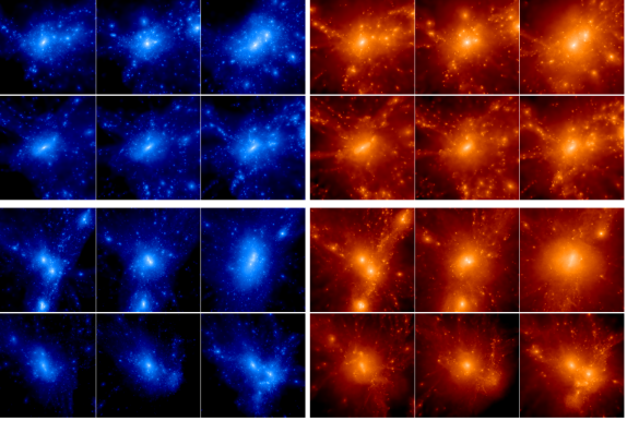
Figure 1: Smoothed projected density images of the high resolution region at $z=0$ centred the two groups used in this study. Q (top two rows) & MM (bottom two rows). From left to right: $\Lambda$CDM, $\phi$CDM, $\phi(\beta=0.05)$CDM. Top row in each subpanel shows CDM distribution and bottom row shows gas distribution. Densities are plotted on a logarithmic scale with bright regions being dense. The scale is arbitrary but kept fixed for a given particle type and halo.

We use 3 cosmologies in this study: a reference $\Lambda$CDM; an uncoupled quintessence model ($\phi$CDM); and one coupled model ($\beta_{o}=0.05$). As mentioned previously all cosmologies have parameters consistent with $z=0$ $\Lambda$CDM Planck data $(h,\Omega_{m},\Omega_{b},\sigma_{8})=(0.67,0.3175,0.049,0.83)$ Planck Collaboration et al. (2013, 2015). Our coupled model is chosen to test the boundaries of allowed coupling (see Pettorino et al., 2012) in order to maximise any observational differences that may exist between this cosmology and the standard $\Lambda$CDM model. The power spectrum and evolution of these quantities along with the growth factor $f\equiv d\ln D(a)/d\ln a$ are calculated using first-order Newtonian perturbation equations and the publicly available Boltzmann code cmbeasy Doran (2005). Initial conditions are produced using a uniform Cartesian grid and a first-order Zel’Dovich approximation using a modified version of the publicly available n-genic code. The modified code uses the growth factors and expansion history calculated by cmbeasy to correctly calculate the particle displacements in the non-standard cosmologies.

We produce several well resolved dark matter haloes using hydrodynamical zoom simulations in the cosmologies mentioned previously. As the N-Body code used here is described in detail in Carlesi et al. (2014a), we briefly summarise the key points here. dark-gadget is a modified version of p-gadget-2. The key modifications are the inclusion of a separate gravity tree to account for the additional long range forces arising from the scalar field, and an evolving dark matter N-body particle mass which models the decay of the dark matter density. The code requires the full evolution of the scalar field, $\phi$, the mass of the dark matter N-body particle, and the expansion history.

The zoom simulations used a parent simulation of $L_{\rm box}=50\ h^{-1}{\rm Mpc}$ containing $2\times 256^{3}$ particles (DM and gas particles) with the following cosmological parameters. Candidate objects were identified using velociraptor Elahi et al. (2011). For each selected object, all particles within a radius of $\sim 3R_{\rm max}$ of the halo at $z=0$ are identified in the high resolution IC that was down sampled to produce the low resolution parent simulation. The mass resolution in the zoom region is $8\times 10^{6}\ h^{-1}{\rm M_{\odot}}$ and $1.5\times 10^{6}\ h^{-1}{\rm M_{\odot}}$ for dark matter and gas particles respectively, or an effective resolution of $1024^{3}$. All the simulations are started at $z=65$ with the same phases in the density perturbations and use a gravitational softening length of $1/40$ of the interparticle spacing. We study our haloes across cosmic time, focusing specifically on $z=0$ and $z=0.5$, where the progenitors of the clusters are large galaxy groups. The cosmological parameters relative to the fiducial $\Lambda$CDM model at $z=0.5$, where the quantities are not normalised, are listed in Table 1.

Table 1: Comparison of several key cosmological parameters relative $\Lambda$CDM at $z=0.5$. Here $m_{\rm DM}$ is dark matter mass, $D_{+}$ is the growth function, $H$ is the Hubble expansion rate, and $G_{\rm eff}$ is the effective gravitational potential in DM-DM interactions.

Cosmology	$\frac{m_{\rm DM}}{m_{{\rm DM}}^{\Lambda{\rm CDM}}}$	$\frac{\Omega_{\rm cdm}}{\Omega_{{\rm CDM}}^{\Lambda{\rm CDM}}}$	$\frac{D_{+}}{D_{+}^{\Lambda{\rm CDM}}}$	$\frac{H}{H^{\Lambda{\rm CDM}}}$	$\frac{G_{\rm eff}}{G_{{\rm eff}}^{\Lambda{\rm CDM}}}$
$\phi$CDM	1	0.979	0.992	1.0129	1
$\phi(\beta=0.05)$CDM	1.0027	0.993	1.009	1.0024	1.0025

We identify all bound haloes and their substructures using velociraptor within the high resolution region. This code identifies field haloes using a 3D Friends-of-Friends (FOF) algorithm with a linking length of $0.2$ times the inter-particle spacing. Substructures are then found by identifying particles that belong to a local velocity distribution that differs from average background and then linking this outlier population using a phase-space FOF approach (for details see Elahi et al., 2011, 2013). This technique not only identifies bound subhaloes, it will also identify the tidal features associated with the subhalo and even completely unbound tidal debris.

3 Haloes in Coupled Cosmologies

Table 2: Bulk Properties of Q & MM: total bound mass $M_{\rm tot}$; total number of particles $N_{p}$; mass within the so-called virial radius $M_{\Delta}=4\pi\Delta\rho_{\rm bg}R_{\Delta}^{3}/3$, where $\Delta=200$; baryon fraction $f_{\rm b}$; maximum circular velocity $V_{\rm max}$; radius of maximum circular velocity $R_{V_{\rm max}}$; number of subhaloes within the virial radius $N_{\rm subs}$; mass fraction in subhaloes $f_{M,{\rm subs}}$; total number of substructures (i.e., both intact and tidally disrupted subhaloes) within the virial radius $N_{\rm S}$; mass fraction in substructures $f_{M,{\rm S}}$; mass fraction in unbound tidal debris $\Delta f_{M,{\rm S,tid}}$.

	Cosmology	$M_{\rm tot}$	$N_{\rm p,DM}$	$M_{\Delta}$	$f_{\rm b}$	$V_{\rm max}$	$R_{V_{\rm max}}$	$R_{\rm\Delta}$	$c_{V_{\rm max}}$	$N_{\rm subs}$	$f_{M,{\rm subs}}$	$N_{\rm S}$	$f_{M,{\rm S}}$	$\Delta f_{M,{\rm S,tid}}$
		[$10^{13}\ {\rm M_{\odot}}$]	$10^{6}$	[$10^{13}\ {\rm M_{\odot}}$]		km/s	kpc	kpc
Q($z=0$)	$\Lambda$CDM	8.25	5.41	6.44	0.132	687	177	865	4.89	1036	0.069	1050	0.098	0.029
	$\phi$CDM	9.39	6.18	7.97	0.125	743	265	930	3.51	1454	0.097	1485	0.135	0.038
	$\phi(\beta=0.05)$CDM	16.00	10.73	11.91	0.119	826	314	1063	3.38	2544	0.122	2599	0.198	0.078
Q($z=0.5$)	$\Lambda$CDM	4.29	2.85	3.40	0.139	629	118	470	3.96	633	0.047	658	0.079	0.032
	$\phi$CDM	4.20	2.76	3.80	0.126	673	193	486	2.51	529	0.071	542	0.102	0.031
	$\phi(\beta=0.05)$CDM	7.52	4.97	6.04	0.130	778	248	567	2.28	960	0.080	991	0.119	0.039
MM($z=0$)	$\Lambda$CDM	3.11	2.09	2.94	0.126	518	207	667	3.21	445	0.033	467	0.094	0.059
	$\phi$CDM	7.04	4.63	6.39	0.127	668	393	864	2.19	1434	0.128	1450	0.244	0.116
	$\phi(\beta=0.05)$CDM	13.85	9.43	11.70	0.117	708	774	1057	1.36	2293	0.077	2336	0.113	0.036
MM($z=0.5$)	$\Lambda$CDM	2.42	1.62	1.94	0.115	501	211	381	1.80	335	0.118	356	0.177	0.059
	$\phi$CDM	2.40	1.61	2.20	0.123	553	170	398	2.33	315	0.068	335	0.142	0.074
	$\phi(\beta=0.05)$CDM	6.07	4.07	3.10	0.117	621	165	446	2.70	385	0.061	415	0.102	0.039

Here we focus on two objects: one with a quiescent history (Q); and one which is undergoing and has undergone several major mergers (MM). These two objects are chosen to explore the effects of coupled dark sector physics in two different dynamical regimes. We show the dark matter & gas distributions at $z=0.0$ & $z=0.5$ in Fig. 1 and list their bulk properties in Table 2.

Focusing on Fig. 1, we see that the quiescent group looks remarkably similar at all times in spite of the fact that $\phi(\beta=0.05)$CDM-Q halo has a maximum circular velocity that $20\%$ higher and is $\approx 80\%$ more massive at $z=0$ that its counterparts in uncoupled simulations. Considering the how self-similar dark matter haloes appear, this fact in itself is not very surprising.

MM on the other hand appears to be at different stages of a major merger. In $\phi(\beta=0.05)$CDM, at $z=0$, the halo is relaxing from the major merger event that occurred at $z=0.5$. Three “cores” are visible, remnants of past mergers. The ongoing merger at $z=0.5$ is the reason for the large differences in the total bound FOF mass of the halo relative to its virial mass seen in Table 2. The MM halo in uncoupled cosmology also has several cores at $z=0$ and is near a similar mass halo which which it will merge in the near future. On the other hand, $\Lambda$CDM-MM has yet to undergo its first major merger, as evidence by its lack of merger remnants.

Clearly for our choice of cosmological parameters, haloes at these mass scales are more massive in strongly coupled cosmologies but can have similar masses in cosmologies with the same dark matter density and physics but different expansion histories and power spectra. Hence, the increase in mass is a result of higher matter densities (particularly at early times), a higher effective gravitational force experienced by dark matter and higher growth functions (see Table 1). This difference is in spite of the fact that these parameters change by a few percent at most, and $\sigma_{8}(z=0)$ is the same in every cosmology. However, larger haloes is not an unambiguous signal of a coupled dark sector. Despite the differences in mass at this particular scale and time, the freedom allowed in the $(\Omega_{m},\sigma_{8})$ plane means that the current differences in the mass of these objects is not necessarily a useful signature of coupled dark matter. For both Q & MM, moving from one cosmology to the next appears to look like viewing the same object at different times. Therefore, it is quite possible that a different viable choice of $(\Omega_{m},\sigma_{8})$ would remove these differences.

None of the properties listed in Table 2 show an unambiguous trend with coupling that is not affected by the merger history. For example, the concentration parameter was found by Carlesi et al. (2014a) to be lower in coupled cosmology. This trend is followed by Q but not by MM at early times. Moreover, even the uncoupled cosmology has a lower concentration for these haloes. The fraction of the host’s mass bound up in subhaloes also varies between cosmologies as does the fraction in tidal debris.

Even sampling the growth of structure across some fraction of cosmic time need not be necessarily effective for the same reason that as the observed mass difference. The weak gravitational lensing study by Pace et al. (2015) & Giocoli et al. (2015) found differences in the convergence power spectrum between $\Lambda$CDM and coupled cosmologies, however, much of the difference arises to different $\sigma_{8}$ normalisations. We therefore study the internal properties of these objects in search of unambiguous probes of coupled dark sector physics.

3.1 Profiles

The first question is whether the density profiles differ. Carlesi et al. (2014b) stacked clusters to measure the average radial density profile at $z=0$ and found negligible differences save in the poorly resolved, inner region for the most strongly coupled cosmology. Based on Fig. 1, it is not obvious major differences will exist for the quiescent Q group but there should be differences in the merging MM group, particularly for $\phi(\beta=0.05)$CDM arising from the dynamical state. The Q quiescent halo profiles shown in Fig. 2 are almost indistinguishable. The residuals do show that the central density of the strongly coupled cosmology is lower than the $\Lambda$CDM one but key is that the residuals are flat. The shape is not systematically different, all are reasonably characterised by NFW (or Einasto) profile (e.g Navarro et al., 1997, 2004).

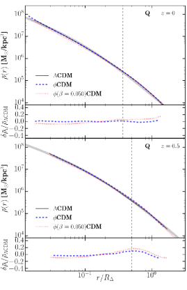
Figure 2: Radial density profiles along with residuals (where we have removed the average offset to emphasise changes in slope) of Q at $z=0$ (top two panels) and at $z=0.5$ (bottom two panels). We show a thick dark gray region showing the best fit NFW profile to the $\Lambda$CDM model and a dashed vertical line at the fitted scale radius.

For MM, shown in Fig. 3, the effects of the merger are clearly visible. The deviation away from an NFW in the central regions of $\phi(\beta=0.05)$CDM-MM at $z=0$ are due to the presence of multiple cores (see Fig. 1, where the cores for MM are very evident). A deviation is also seen in the uncoupled model. The profile of $\phi(\beta=0.05)$CDM-MM at $z=0.5$ also extends to much larger radii, a result of the major merger taking place, with the smaller group residing just past $R_{\Delta}$. Of greater importance is the similarity in the shape of the profiles at $z=0.5$, when the main halo is relatively undisturbed in all three cosmologies. Again, the cosmologies have produced haloes which are remarkably similar. Even the shallower interior slopes in coupled cosmologies noted for Q and in previous studies of relaxed haloes is not seen here as it has been affected by the dynamical state of the system.

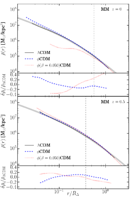
Figure 3: Same as Fig. 2 but for MM.

Given that the effective gravitational field experienced by dark matter differs from that of baryons in coupled cosmologies, one might expect a difference in the distribution of baryons, which is shown in Fig. 4. Unfortunately, there is a great deal of disparity between the cosmologies and little indication that on an individual object basis, the baryons can be used to discriminate between uncoupled and coupled dark matter physics, even in simplistic adiabatic simulations. By looking at various times and dynamical state, we can clearly see that differences in accretion history are of greater importance than a coupled dark sector.

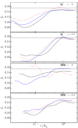
Figure 4: Radial baryon fractions of Q (top two panels, with upper for $z=0$, lower for $z=0.5$) and MM (bottom two). Line styles and colours are the same as in Fig. 2.

4 Subhaloes: Coupled cosmologies in high density environments

The bulk host haloes properties show few unambiguous differences between uncoupled and coupled cosmologies. Here we examine if subhaloes, which will host galaxies of similar mass to the Milky Way, show major differences. We first focus on the subhalo population residing within the high density environment inside the virial radius of the host haloes, Q & MM.

4.1 Mass distribution

The simplest comparison to make is with the subhalo mass distribution, shown in Fig. 5-6. Note that we do not classify the main merging halo in the $\phi(\beta=0.05)$CDM-MM simulation at $z=0.5$ as a “subhalo” and so it is not present in this figure. Remarkably, the shape of the subhalo mass function is unaffected by the differences in the initial power spectra, expansion histories and, at first glance, even the dynamical state of the host halo! This result is seen in the lower subpanels of each figure. The residual $\delta n_{\rm i}/n_{\rm\Lambda CDM}=n_{\rm i}/n_{\rm\Lambda CDM}-\left\langle n_{\rm i}/n_{\rm\Lambda CDM}\right\rangle$, has the average amplitude difference between models, $\left\langle n_{\rm i}/n_{\rm\Lambda CDM}\right\rangle$, removed to emphasise differences in the slope. The residuals at masses above the resolution limit, although noisy, are relatively flat or show little systematic tilt, at least for $z=0$. At $z=0.5$, the coupled cosmology is tilted relative to the uncoupled cosmologies. However, this tilt is not systematic, in one halo, the mass function is steeper, in the other it is flatter. Moreover, this difference is it present at even higher redshifts (not shown here for brevity). Clearly the shape of the subhalo mass distribution, which would be an ideal signature, is primarily governed by nonlinear dynamics (mass loss, dynamical friction, etc.), rather than cosmologically dependent quantities such as the accretion rate or the small difference in the gravitational force experienced by dark matter.

The top subpanels of this figure also indicate that the differences in the number of and mass fractions within subhaloes seen in Table 2 are not informative as the differences in the amplitude of the mass distribution curves are negligible and not correlated with the underlying cosmological model. Coupled cosmologies, at least for $\beta\leq 0.05$ are not intrinsically richer or poorer than their uncoupled counterparts.

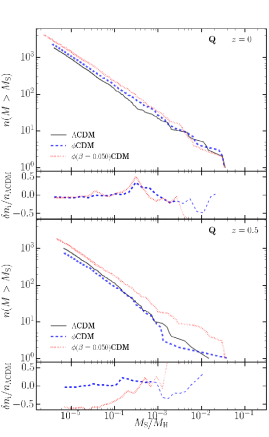
Figure 5: The $z=0$ cumulative mass function along (large panels) with the residuals in the cumulative number (smaller panels) for Q (top two panels) and MM (bottom two panels). In the smaller panels showing the ratio, thin lines correspond to where $n_{i}$ & $n_{\Lambda{\rm CDM}}$ $\leq 10$, i.e., where the statistics are poor. Line styles and colours are the same as in Fig. 2

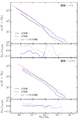
Figure 6: Same as Fig. 5 but for MM.

4.2 Concentration

We next examine the concentration of subhaloes in Fig. 7, specifically the mass dependence of ratio between the virial radius relative to the maximum circular velocity radius, $c_{V_{\rm max}}$ (we only show $z=0$ for brevity as $z=0.5$ is similar). There does appear to be a trend for coupled cosmologies to have less concentrated subhaloes, particularly at smaller masses, in agreement with previous studies Baldi et al. (2010); Carlesi et al. (2014a). The variation in $c_{V_{\rm max}}$ at a given mass is large, possibly masking this difference. Moreover, although some of the reduced concentration in the coupled simulation is due to the extra fictional force experienced by dark matter, some of it will also be driven by different expansion histories. The concentration of a halo depends in part on the formation time of the object (e.g. Bullock et al., 2001; Ludlow et al., 2014) and is also affected by the dynamical state of a (sub)halo.

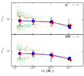
Figure 7: The mass-concentration relation at $z=0$. We first bin the data in mass and calculate the median and the $16\%$ & $84\%$ quantiles of $c_{V_{\rm max}}$ in each bin. These are plotted in the large solid points with error bars. We also plot the outlying points as small points. Line styles and colours are the same as in Fig. 2, markers are: $\Lambda$CDM circle, $\phi$CDM square, $\phi(\beta=0.05)$CDM diamond. Outlying point colours are: $\Lambda$CDM grey, $\phi$CDM cyan, $\phi(\beta=0.05)$CDM orange. The x position of the bins are offset by an small arbitrary amount between each cosmology for clarity. As quantiles are misleading for a small sample, we do not plot error bars for bins containing fewer than 5 points, instead, we plot all the points in the bin and the median of these points.

If we turn our attention more directly observable quantities, that is $V_{\rm max}-R_{V_{\rm max}}$ in Fig. 8, the differences are less evident. Subhaloes are more extended at a given $V_{\rm max}$ in $\Lambda$CDM relative to $\phi$CDM. Although including coupling has moved the subhalo distribution closer to the $\Lambda$CDM one, the fact that the quintessence model can differ from the $\Lambda$CDM model suggests that the concentration of subhaloes is not an ideal indicator of a coupled dark sector.

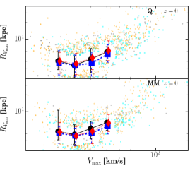
Figure 8: The $V_{\rm max}-R_{V_{\rm max}}$ distribution similar to Fig. 7.

4.3 Angular momentum

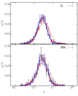
Figure 9: Subhalo spin distribution at $z=0$. For reference we also show the subhalo spin distribution from Onions et al (2013) for subhaloes from a dark matter only simulation of a $10^{12}\ {\rm M_{\odot}}$ halo by a solid gray line. Onions et al (2013) found that subhaloes peaks at a lower spin value than the halo distribution. Probabilities and errors are estimate using bootstrap resampling. Line styles and colours are the same as in Fig. 2.

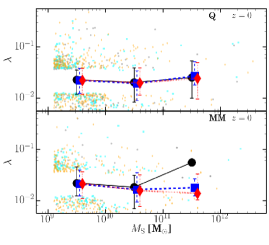
Figure 10: Spin as a function of mass. Format similar to Fig. 7.

The angular momentum of field haloes in non-standard cosmologies shows indications that there maybe subtle differences in the peak of the spin parameter distribution (e.g. Hellwing et al., 2013; Carlesi et al., 2014b). Here we examine the spin parameter as defined by Bullock et al. (2001),

$$\lambda=\frac{L}{\sqrt{2}MVR},$$ (4)

where $L$ is the angular momentum, $M$ is the total mass, and $R$ is the radius of the subhalo, and $V^{2}=GM/R$. Normally, these quantities are measured at the so-called virial radius, $R_{\Delta}$, however, subhaloes can be truncated at overdensities higher that $\Delta$. For those subhaloes, we use the total mass, angular momentum and size of the object to calculate $\lambda$.

Figure 9 shows the total distribution across all mass scales. Note that we have calculated spins using the self-bound portions of a substructures, that is we do not include the loosely unbound tidal tails associated with subhaloes and ignore tidal debris, which would produce a longer high spin tail. First we note that the subhalo spin distribution here is lower than that found in Onions et al. (2013), who studied subhaloes in a galaxy mass host. The spin distribution at higher redshifts and lower host masses is in better agreement with Onions et al. (2013).

The major feature of this plot is the absence of systematic difference in the distributions between uncoupled and coupled cosmologies. There is a hint in a shift towards higher spins in this coupled cosmology, there being a small deficit in probability relative to the uncoupled cosmologies just below the peak of the distribution and a possible excess above. However, the differences are not incredibly significant. A simple two-sided Kolmogorov–Smirnov (KS) test comparing the distributions returns p-values of $\gtrsim 0.5$, regardless of which two cosmologies are compared, that is the empirical distributions arise from the same parent distribution. This is also true at higher redshifts. Moreover, the difference is more noticeable in Q than in MM, showing the dynamical state of the host does influence the spins of subhaloes residing in it.

Even separating the distribution into masses, as we do in Fig. 10, does not necessarily show an unambiguous signature of a coupled dark sector. Small coupled cosmology subhaloes of have marginally higher spins. However, even the uncoupled cosmology differs from $\Lambda$CDMand for the well sampled mass scales, the mass dependence of $\lambda$ shows little difference between cosmologies with the two-sided KS-test giving p-values of $\gtrsim 0.4$ regardless of mass bin used. Moreover, the spin parameter is influenced by galaxy formation physics, which we have not included in our simulations. The effect of forming stars is likely to wash out the small differences noted here.

4.4 Alignment

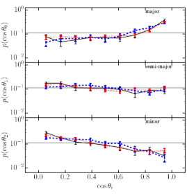
Figure 11: Subhalo alignment with the axes of the host halo for Q at $z=0$. We show the probability for a isotropically distributed distribution by a gray line. Probabilities and errors are estimated using bootstrap resampling. Line styles and colours are the same as in Fig. 2.

Observations suggests that subhaloes/satellite galaxies are anisotropically distributed within there host halo. $\Lambda$CDM simulations naturally give rise to anisotropic subhalo populations, however, this cosmology struggles to explain the strength of the alignments observed. Here we examine if a coupled dark sector produces a more anisotropically distributed subhalo population via the angle between a subhalo’s position, ${\bf x}$, and major, semi-major, and minor axes of the host halo defined by the eigenvectors $e_{i}$ of the reduced inertia tensor Dubinski & Carlberg (1991); Allgood et al. (2006),

$$\tilde{I}_{j,k}=\sum\limits_{n}\frac{m_{n}x^{\prime}_{j,n}x^{\prime}_{k,n}}{(r^{\prime}_{n})^{2}}.$$ (5)

Here the sum is over particles in the halo, $(r^{\prime}_{n})^{2}=(x^{\prime}_{n})^{2}+(y^{\prime}_{n}/q)^{2}+(z^{\prime}_{n}/s)^{2}$ is the ellipsoidal distance between the subhalo’s centre of mass and the $n$th particle, primed coordinates are in the eigenvector frame of the reduced inertia tensor, and $q$ & $s$ are the semi-major and minor axis ratios respectively.

We show in Fig. 11 the distribution of $\cos\theta_{i}={\bf x}\cdot{\bf e}_{i}/x$ for Q at $z=0$. This figure indicates subhaloes are typically aligned along the major axis of the host halo. However, haloes in coupled cosmologies do not have subhalo populations that are any more or less anisotropic than those in uncoupled cosmologies. Despite the vary different dynamical state of MM between cosmologies and relative to Q, the overall picture is similar. The subtle difference is that subhaloes are not as strongly aligned/anti-aligned to the major/minor axis of the host halo, a result of the violent phase-mixing in major mergers and randomisation of orbits. This type of analysis in itself does not indicate whether or not coupled cosmologies produce planar arrangement of satellites.

To see if planes are present we examine the distributions of distances to the three planes with normal vectors defined by the inertia tensor’s eigenvectors. This distribution is compared to an isotropically distributed subhalo population with the same overall radial distribution present in the halo. We show for Q the ratio relative to the isotropic expectation normalised by the uncertainty, $\delta p/\sigma=(p_{\rm obs}/p_{\rm iso}-1)/\sigma(p_{\rm obs}/p_{\rm iso})$, as function of distance in Fig. 12.

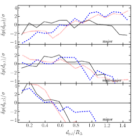
Figure 12: Relative probability distribution of distances to three planes normalised by the variance in the observed PDF for Q at $z=0$. The expectation value for an isotropic distribution is shown by a gray line. Probabilities and errors are estimated using bootstrap resampling. Line styles and colours are the same as in Fig. 2.

A planar structure would show up as an excess in the probability of finding subhaloes at small distances from a given plane. Focusing on the “major” plane, that which is perpendicular to the major axis that has a normal vector along the major axis, we see that the population is generally consistent with an isotropic distribution (within $2\sigma$). There is a hint of a deficit of objects at small projected distances that is matched by the increase in the number of subhaloes with small projected distances orthogonal to this plane. In general, $\lesssim 2\sigma$ deviations occur at all distances from the planes examined here, arising from the overall anisotropic distribution of subhaloes. The exception is the “minor” plane, which shows $\gtrsim 3\sigma$ deviation away from an isotropic distribution at small projected distances for all three cosmologies.

Focusing on $\Lambda$CDM-Q, there are 198 subhaloes ($20\%$ of the subhaloes composed of $\geq 100$ particles) within a projected distance of $40$ kpc from the “minor” plane spanning a range of radii, from $280$ kpc to $1600$ kpc, that is from $\sim R_{V_{\rm max}}$ to past $\sim 2R_{\Delta}$. However, this planar structure is purely spatial, it is not a dynamically stable structure. The angular momentum of the subhaloes not strongly aligned with the normal vector defining the plane ($45^{\circ}$). Subhalo’s are as likely to have tangentially dominated velocities as radial ones and be rotating, counter-rotating or have an orbit principally out of the plane. The velocity dispersions perpendicular to the plane for even the coldest $40\%$ is $\sim 200$ km/s, meaning this plane would disperse within $200$ Myr. As expected, $\Lambda$CDM haloes have anisotropic distributions of subhaloes but no planes.

At first glance the inclusion of coupling looks encouraging. The deviations away from projected distances of an isotropically distributed subhalo population are more significant, although it is still contains similar fractions of the subhalo population as $\Lambda$CDM($\approx 20\%$). This planar structure has a vertical distribution of $\sim 70~{}$kpc, an angular extent of $\sim 180^{\circ}$, and spans $\sim 2~{}$Mpc in radius. However, its dynamics again show the transient nature of this plane. Its angular momentum axis is misaligned with the plane by $70^{\circ}$ and the vertical velocities are offset from the plane by $130$ km/s and will disperse within $\sim 190$ Myr. The main component of this plane is two groups of subhaloes, which at $z=0.5$ reside in the two main filaments that connect this halo’s progenitor to the cosmic web.

MM, despite being at various points in a merger in the different cosmologies has similar features: anisotropic subhalo distribution and no dynamically stable planar structures. This trend is true for both haloes at earlier redshifts as well. It is however interesting to note that the statistical significance of a flatten spatial distribution in the “minor” plane is always higher in the coupled cosmology.

That is not to say spatially compact planes do not exist in other cosmologies. We note that at $z=1$ both $\phi$CDM & $\phi(\beta=0.05)$CDM Q haloes (with $M\approx 3.5\times 10^{13}\ {\rm M_{\odot}}$) have “minor” planes of satellites spanning $40$ kpc with an orbital angular momentum axis aligned with the plane’s normal vector, although the motions orthogonal to the plane are large enough ($200$ km/s) to disperse the plane within a $\sim 200$ Myr. Despite the high redshift, these host masses are closer to the mass scale of the Local Group, where planes have been observed.

5 Field Haloes: Coupled cosmologies in lower density environments

The dense environment within a group appears to show little differences in the subhalo population. However it is worthwhile examining whether this is true in all environments. We therefore examine the bulk properties of haloes that lie outside the group as a function of the distance from the centre of the host. As the haloes are triaxial and we are interested in exploring environments at different densities, we use the ellipsoidal distance to the halo centre, $r^{\prime}=(x^{2}+y^{2}/q^{2}+z^{2}/s^{2})$, where coordinates are in the eigenvector frame of the reduced inertia tensor, and $q$ & $s$ are the axis ratios (which for Q are $q\sim 0.75$ & $s\sim 0.47$), instead of the pure radial distance.

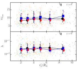
Figure 13: Properties of haloes around Q verses ellipsoidal distance, $r^{\prime}$. Here we show the spin, $\lambda$ and concentration $c_{V_{\rm max}}$ (top and bottom respectively). We select haloes with masses $5\times 10^{9}/\ {\rm M_{\odot}}\leq M\leq 5\times 10^{10}\ {\rm M_{\odot}}$, as these quantities depend on host halo mass. Format is similar to Fig. 7.

Figure 13 shows the concentration and spin of small haloes around Q, the halo with the quiescent merger history. This figure shows haloes differ between cosmologies. Focusing on the top panel of Fig. 13, we find haloes are more concentrated in the quintessence cosmology than in $\Lambda$CDM. Adding coupling has reversed the trend in $c_{V_{\rm max}}$, resulting in increasingly less concentrated haloes. The spin distribution to show little dependence on on its environment but this is due to the strict removal of unbound particles. If we include loosely unbound particles within the FOF envelope of field haloes we would clearly see that haloes closer in have higher $\lambda$, a result of becoming tidally disrupted. More importantly, there is little difference between cosmologies in the different environments. These trends apply to MM, despite its active merger history.

As baryons and dark matter do not feel the same gravitational force, we examine the baryon fractions of haloes and the dependence upon environment in Fig. 14 for both Q & MM. The first notable feature is the difference between the median $f_{\rm b}$ in Q and MM for the same cosmology. Here the dynamical state and the density of the local environment has affected the median $f_{\rm b}$ at a given $r^{\prime}$, although the overall trends remain unchanged. Small haloes have decreasing $f_{\rm b}<\Omega_{b}/\Omega_{m}$ with decreasing radius as the hot gas surrounding the cluster strips haloes with increasing efficiency the closer a halo is to group centre. Of greater importance is the apparent decrease in $f_{\rm b}$ when $\beta>0$. The exact median baryon fraction depends on the dynamical state but coupling decreases the radius at which there are significant drop in $f_{\rm b}$. The complication lies in the radius at which this occurs. Q haloes show a more gradual change and baryon poor subhaloes appear at much larger distances than in MM. Additionally, the surrounding halo population in $\Lambda$CDM-MM is strongly effected the the presence of another infalling group mass halo, hence the sudden drop in the median $f_{\rm b}$ and number of subhaloes containing any baryons at all.

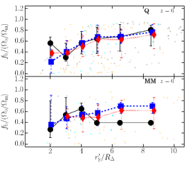
Figure 14: Baryon fraction normalised by the cosmic baryon fraction, $f_{\rm b}/(\Omega_{b}/\Omega_{m})$, for Q (top) & MM (bottom). Similar to Fig. 13.

6 Discussion & Conclusion

We have studied the internal properties of group mass haloes in coupled Dark Energy-Dark Matter cosmologies using adiabatic zoom simulations. The cosmologies used in this study consist of a fiducial $\Lambda$CDM model, a quintessence model, and a strongly coupled DEDM model, $\phi(\beta=0.05)$CDM. In coupled models, dark matter decays into dark energy, giving rise to the late time accelerated expansion, an additional frictional force experienced by DM, and expansion histories and growth functions that differ from $\Lambda$CDM. It is important to note that the best fit parameters for a given alternative cosmology to the CMB will differ from the best fit parameters of $\Lambda$CDM. Given this freedom, we have chosen to pin our simulations at $z=0$ so that the density parameters and $\sigma_{8}$ match the $\Lambda$CDM values based on $\Lambda$CDM results from Planck.

Our approach was to examine in detail two well resolved cluster mass haloes with different dynamical states to identify unambiguous signatures of a coupled dark sector. We find that, considering the differences between $\Lambda$CDM & $\phi$CDM, the two uncoupled cosmologies, haloes that form in the coupled cosmologies appear remarkably similar to $\Lambda$CDM ones, even in instances where the total mass differs by $80\%$. The density profiles of our two well resolved haloes are well characterised by an NFW (or Einasto) like profile when examined at times when the haloes are relaxed. The baryonic fraction profiles of these two haloes vary significantly but not in a systematic way between cosmologies.

The surprising result is the similarity in the subhalo populations of these haloes. The form of the cumulative subhalo mass function is seemingly unaffected by the inclusion of extra dark sector physics. We do find that both subhaloes and small haloes in the outskirts of the group are less concentrated on average in coupled cosmologies. If we look at differences in the $V_{\rm max}-R_{V_{\rm max}}$ plane, which is more directly observable, we find subhaloes with small circular velocities are typically more extended in coupled cosmologies. Unfortunately, a halo’s concentration partially depends on its formation time and thus depends on the choice of cosmological parameters and when a comparison between cosmologies is made. Furthermore, as the concentration of subhaloes can drastically change with the inclusion of galaxy formation physics, which we did not include, this probe of a coupled dark sector is not ideal.

We have also examined these haloes to see if a spatially compact planar arrangement of satellites is present given the observed distributions of satellites around the only two galaxies in which these types of observations are possible, our Galaxy and M31 (e.g. Pawlowski et al., 2012; Ibata et al., 2013; Conn et al., 2013). In all the cosmologies studied here, we do not find strong evidence for a subpopulation of satellites residing in a stable co-rotating plane. However, we do find for both haloes at multiple epochs, our coupled cosmology is more likely to have a statistically significant “planes”. Unfortunately, these are not dynamically stable and will dispersing in roughly $\sim 200$ Myr. These dynamically unstable planar structures are a natural outcome of cosmic structure formation (e.g. Sawala et al., 2014; Libeskind et al., 2015): Subhaloes are principally accreted along filaments. The current tension with observations lies in the how compact these planes are (thicker than observations suggest) and the fact that they do not have strongly correlated velocities. However, the increase in the statistical significance of planar like arrangement of subhaloes in strongly coupled groups is intriguing and warrants further study. Higher filamentary accretion should increase the likelihood of observing planar structures. Thus clues for a coupled dark sector may lie in the amount of material accreted along filaments. Whether there is an increase the observed velocity correlation between satellites relative to $\Lambda$CDM and in better agreement with observation of Ibata et al. (2014) remains to be seen. A complete study of the growth of filaments and the accretion history of haloes is beyond the scope of this paper and will be pursued in the future.

We have also looked for signatures of a coupled dark sector in haloes residing well outside the highly nonlinear cluster environment. Although these haloes show the same trends in their bulk properties as a function of cosmology, i.e., lower concentrations in coupled cosmologies, there is little dependence on environment unique to coupled dark sector physics. The only environmental signature noted lies in the baryon fractions: outlying haloes of a cluster are more likely to have lower $f_{\rm b}$ than their uncoupled counterparts at the same ellipsoidal distance or same environment. The distance (or density) at which there is a significant decrease in the average baryon fractions occurs at moderately larger radii in coupled cosmologies. However, this signature is subtle and is not noticeable when examining baryon fractions as a function of radial (or projected distance) distance to the group centre. Moreover, we have neglected all the complexity associated with galaxy formation physics and the exact treatment of gas and subgrid physics significantly effects the ability of similar mass haloes to retain gas in a given environment (e.g. Tasker et al., 2008; Scannapieco et al., 2012; Sembolini et al., 2015).

Thus, the internal properties of haloes are seemingly indifferent to a coupled dark sector, presenting an interesting possibility: that moderately coupled dark sector models are viable and this physics could just be hidden from view.

References

- Abazajian et al. (2009) Abazajian K. N. et al., 2009, ApJS, 182, 543
- Allgood et al. (2006) Allgood B., Flores R. A., Primack J. R., Kravtsov A. V., Wechsler R. H., Faltenbacher A., Bullock J. S., 2006, MNRAS, 367, 1781
- Amendola (2000) Amendola L., 2000, Phys. Rev. D, 62, 043511
- Anderson et al. (2014) Anderson L. et al., 2014, MNRAS, 441, 24
- Angulo & White (2010) Angulo R. E., White S. D. M., 2010, MNRAS, 405, 143
- Armendariz-Picon et al. (2001) Armendariz-Picon C., Mukhanov V., Steinhardt P. J., 2001, Phys. Rev. D, 63, 103510
- Baldi (2012) Baldi M., 2012, MNRAS, 422, 1028
- Baldi et al. (2010) Baldi M., Pettorino V., Robbers G., Springel V., 2010, MNRAS, 403, 1684
- Bennett et al. (2013) Bennett C. L. et al., 2013, ApJS, 208, 20
- Benson et al. (2002) Benson A. J., Frenk C. S., Lacey C. G., Baugh C. M., Cole S., 2002, MNRAS, 333, 177
- Bertone et al. (2005) Bertone G., Hooper D., Silk J., 2005, Phys. Rep., 405, 279
- Beutler et al. (2011) Beutler F. et al., 2011, MNRAS, 416, 3017
- Beutler et al. (2012) Beutler F. et al., 2012, MNRAS, 423, 3430
- Blake et al. (2011) Blake C. et al., 2011, MNRAS, 418, 1707
- Brax & Martin (2000) Brax P., Martin J., 2000, Phys. Rev. D, 61, 103502
- Bullock et al. (2001) Bullock J. S., Kolatt T. S., Sigad Y., Somerville R. S., Kravtsov A. V., Klypin A. A., Primack J. R., Dekel A., 2001, MNRAS, 321, 559
- Bullock et al. (2000) Bullock J. S., Kravtsov A. V., Weinberg D. H., 2000, ApJ, 539, 517
- Carlesi et al. (2014a) Carlesi E., Knebe A., Lewis G. F., Wales S., Yepes G., 2014a, MNRAS
- Carlesi et al. (2014b) Carlesi E., Knebe A., Lewis G. F., Yepes G., 2014b, MNRAS
- Clarkson et al. (2012) Clarkson C., Ellis G. F. R., Faltenbacher A., Maartens R., Umeh O., Uzan J.-P., 2012, MNRAS, 426, 1121
- Conley et al. (2011) Conley A. et al., 2011, ApJS, 192, 1
- Conn et al. (2013) Conn A. R. et al., 2013, ApJ, 766, 120
- De Boni et al. (2011) De Boni C., Dolag K., Ettori S., Moscardini L., Pettorino V., Baccigalupi C., 2011, MNRAS, 415, 2758
- de Felice & Tsujikawa (2010) de Felice A., Tsujikawa S., 2010, Living Reviews in Relativity, 13, 3
- Dolag et al. (2004) Dolag K., Bartelmann M., Perrotta F., Baccigalupi C., Moscardini L., Meneghetti M., Tormen G., 2004, A&A, 416, 853
- Doran (2005) Doran M., 2005, J. Cosmology Astropart. Phys, 10, 11
- Dubinski & Carlberg (1991) Dubinski J., Carlberg R. G., 1991, ApJ, 378, 496
- Elahi et al. (2013) Elahi P. J. et al., 2013, MNRAS, 433, 1537
- Elahi et al. (2014) Elahi P. J., Mahdi H. S., Power C., Lewis G. F., 2014, MNRAS, 444, 2333
- Elahi et al. (2011) Elahi P. J., Thacker R. J., Widrow L. M., 2011, MNRAS, 418, 320
- Ellis et al. (1984) Ellis J., Hagelin J. S., Nanopoulos D. V., Olive K., Srednicki M., 1984, Nuclear Physics B, 238, 453
- Ferreira & Joyce (1997) Ferreira P. G., Joyce M., 1997, Physical Review Letters, 79, 4740
- Frenk & White (2012) Frenk C. S., White S. D. M., 2012, Annalen der Physik, 524, 507
- Gillet et al. (2015) Gillet N., Ocvirk P., Aubert D., Knebe A., Libeskind N., Yepes G., Gottlöber S., Hoffman Y., 2015, ApJ, 800, 34
- Giocoli et al. (2015) Giocoli C. et al., 2015, ArXiv e-prints
- Hellwing et al. (2013) Hellwing W. A., Cautun M., Knebe A., Juszkiewicz R., Knollmann S., 2013, J. Cosmology Astropart. Phys, 10, 12
- Heymans et al. (2013) Heymans C. et al., 2013, MNRAS, 432, 2433
- Hu & Sawicki (2007) Hu W., Sawicki I., 2007, Phys. Rev. D, 76, 064004
- Huey & Wandelt (2006) Huey G., Wandelt B. D., 2006, Phys. Rev. D, 74, 023519
- Ibata et al. (2014) Ibata N. G., Ibata R. A., Famaey B., Lewis G. F., 2014, Nature, 511, 563
- Ibata et al. (2013) Ibata R. A. et al., 2013, Nature, 493, 62
- Kilbinger et al. (2013) Kilbinger M. et al., 2013, MNRAS, 430, 2200
- Klypin et al. (1999) Klypin A., Gottlöber S., Kravtsov A. V., Khokhlov A. M., 1999, ApJ, 516, 530
- Klypin et al. (2003) Klypin A., Macciò A. V., Mainini R., Bonometto S. A., 2003, ApJ, 599, 31
- Kowalski et al. (2008) Kowalski M. et al., 2008, ApJ, 686, 749
- Li & Barrow (2011) Li B., Barrow J. D., 2011, Phys. Rev. D, 83, 024007
- Li et al. (2013) Li Z., Wang Y., Yang X., Chen X., Xie L., Wang X., 2013, ApJ, 768, 20
- Libeskind et al. (2015) Libeskind N. I., Hoffman Y., Tully R. B., Courtois H. M., Pomarede D., Gottloeber S., Steinmetz M., 2015, ArXiv e-prints
- Lovell et al. (2014) Lovell M. R., Frenk C. S., Eke V. R., Jenkins A., Gao L., Theuns T., 2014, MNRAS, 439, 300
- Ludlow et al. (2014) Ludlow A. D., Navarro J. F., Angulo R. E., Boylan-Kolchin M., Springel V., Frenk C., White S. D. M., 2014, MNRAS, 441, 378
- Macciò et al. (2004) Macciò A. V., Quercellini C., Mainini R., Amendola L., Bonometto S. A., 2004, Phys. Rev. D, 69, 123516
- Mead & Peacock (2014) Mead A. J., Peacock J. A., 2014, MNRAS, 440, 1233
- Moore et al. (1999) Moore B., Ghigna S., Governato F., Lake G., Quinn T., Stadel J., Tozzi P., 1999, ApJ, 524, L19
- Navarro et al. (1997) Navarro J. F., Frenk C. S., White S. D. M., 1997, ApJ, 490, 493
- Navarro et al. (2004) Navarro J. F. et al., 2004, MNRAS, 349, 1039
- Nickerson et al. (2011) Nickerson S., Stinson G., Couchman H. M. P., Bailin J., Wadsley J., 2011, MNRAS, 415, 257
- Nickerson et al. (2012) Nickerson S., Stinson G., Couchman H. M. P., Bailin J., Wadsley J., 2012, MNRAS, 285
- Onions et al. (2013) Onions J. et al., 2013, MNRAS, 429, 2739
- Pace et al. (2015) Pace F., Baldi M., Moscardini L., Bacon D., Crittenden R., 2015, MNRAS, 447, 858
- Pawlowski et al. (2012) Pawlowski M. S., Pflamm-Altenburg J., Kroupa P., 2012, MNRAS, 423, 1109
- Petraki & Volkas (2013) Petraki K., Volkas R. R., 2013, International Journal of Modern Physics A, 28, 30028
- Pettorino et al. (2012) Pettorino V., Amendola L., Baccigalupi C., Quercellini C., 2012, Phys. Rev. D, 86, 103507
- Planck Collaboration et al. (2013) Planck Collaboration et al., 2013, ArXiv e-prints
- Planck Collaboration et al. (2015) Planck Collaboration et al., 2015, ArXiv e-prints
- Power (2013) Power C., 2013, Publications of the Astronomical Society of Australia, 30, 53
- Ratra & Peebles (1988) Ratra B., Peebles P. J. E., 1988, Phys. Rev. D, 37, 3406
- Reid et al. (2010) Reid B. A. et al., 2010, MNRAS, 404, 60
- Rozo et al. (2010) Rozo E. et al., 2010, ApJ, 708, 645
- Sawala et al. (2014) Sawala T. et al., 2014, ArXiv e-prints
- Scannapieco et al. (2012) Scannapieco C. et al., 2012, MNRAS, 423, 1726
- Schneider et al. (2014) Schneider A., Anderhalden D., Macciò A. V., Diemand J., 2014, MNRAS, 441, L6
- Sembolini et al. (2015) Sembolini F. et al., 2015, ArXiv e-prints
- Starobinsky (1980) Starobinsky A. A., 1980, Physics Letters B, 91, 99
- Sutter et al. (2015) Sutter P. M., Carlesi E., Wandelt B. D., Knebe A., 2015, MNRAS, 446, L1
- Suzuki et al. (2012) Suzuki N. et al., 2012, ApJ, 746, 85
- Tasker et al. (2008) Tasker E. J., Brunino R., Mitchell N. L., Michielsen D., Hopton S., Pearce F. R., Bryan G. L., Theuns T., 2008, MNRAS, 390, 1267
- Tegmark et al. (2004) Tegmark M. et al., 2004, Phys. Rev. D, 69, 103501
- Tsujikawa (2013) Tsujikawa S., 2013, Classical and Quantum Gravity, 30, 214003
- Vikhlinin et al. (2009) Vikhlinin A. et al., 2009, ApJ, 692, 1060
- Wetterich (1988) Wetterich C., 1988, Nuclear Physics B, 302, 668
- Wetterich (1995) Wetterich C., 1995, A&A, 301, 321
- Yang et al. (2006) Yang X., van den Bosch F. C., Mo H. J., Mao S., Kang X., Weinmann S. M., Guo Y., Jing Y. P., 2006, MNRAS, 369, 1293