Abstract. Recently, $L_{1}$ regularization have been attracted extensive attention and successfully applied in mean-variance portfolio selection for promoting out-of-sample properties and decreasing transaction costs. However, $L_{1}$ regularization approach is ineffective in promoting sparsity and selecting regularization parameter on index tracking with the budget and no-short selling constraints, since the 1-norm of the asset weights will have a constant value of one. Our recent research on $L_{1/2}$ regularization has found that the half thresholding algorithm with optimal regularization parameter setting strategy is the fast solver of $L_{1/2}$ regularization, which can provide the more sparse solution. In this paper we apply $L_{1/2}$ regularization method to stock index tracking and establish a new sparse index tracking model. A hybrid half thresholding algorithm is proposed for solving the model. Empirical tests of model and algorithm are carried out on the eight data sets from OR-library. The optimal tracking portfolio obtained from the new model and algorithm has lower out-of-sample prediction error and consistency both in-sample and out-of-sample. Moreover, since the automatic regularization parameters are selected for the fixed number of optimal portfolio, our algorithm is a fast solver, especially for the large scale problem.

Keywords: Index tracking; $L_{1/2}$ regularization; Half thresholding algorithm.

AMS Subject Classifications:

1 Introduction

Stock index derivatives, such as index funds, index futures, index options etc, have developed very rapidly and become important tools in investment and risk management of global financial markets, especially it shows the better effects to stabilize the stock market in global fiance crisis. Index tracking (e.g., index replication) plays a core role in product design and risk management of index derivatives. It consists in construction of a tracking portfolio whose behavior is as similar as possible to target index during a predefined period.

Broadly speaking, two different strategies can be used to track a given stock market index: the full replication and the non-full replication. The full replication consists in purchasing all constituent stocks of a given index. In practice, this strategy need high transaction costs. An alternative way is the non-full replication, which include the stratified sampling replication and the optimal replication. Since the selection of the stocks in stratified sampling replication depends on the manager’s experience, so the tracking portfolio is non-optimal, thus we focus on the optimal replication method in this paper. The optimal replication aims to find the portfolio that minimizes the tracking error by investing in only a subset of the assets using optimization method. This strategy involves much lower transaction costs, and can achieve acceptable tracking errors in principle.

Different quantitative methods have been proposed to tackle such an optimization problem. Roll establishes optimal index tracking models and proposed a mean-variance analysis of index tracking on Markowitz’s earlier study [25]. Tabata and Takeda discuss the index fund management based on mean-variance model [29]. Buckley and Korn apply optimal impulse control techniques to the index tracking problem with fixed and proportional transaction costs [6]. Rudolf et al. propose several piecewise linear measures of the tracking error, and solve the problem by means of linear programming [26]. Alexander proposes the construction of tracking portfolios by analyzing the coincidental structure between the time series of each of the assets and the time series of the tracked index [1]. Ammann and Zimmermann investigate the relationship between several statistical measures of tracking error and asset allocation restrictions based on admissible weight ranges [2]. Gilli and Kellezi propose the use of the threshold accepting heuristic to solve the problem, including cardinality restrictions and transaction costs [18]. Beasley et al. address the index tracking problem using evolutionary heuristics with real-valued chromosome representations [4] . Lobo et al. investigate the portfolio optimization problem with transaction costs, which they address by means of a heuristic relaxation method that consists in solving a small number of convex optimization problems using fixed transaction costs [22]. Torrubiano and Beasley present a nonlinear mixed-integer optimal model and a corresponding algorithm for index tracking [7]. Torrubian et al. design a hybrid strategy that combines an evolutionary algorithm with quadratic programming to yield the optimal tracking portfolio that invests only in the selected assets [30].

On the other hand, statistical regularization methods have been successfully applied in mean-variance portfolio selection in order to promote the identification of sparse portfolios with good out-of-sample properties and low transaction costs [13, 5, 16]. DeMiguel et al focuses on the effect of the constraints on the covariance regularization, a technique extension of the result in Jagannathan and Ma [20]. Brodie et al emphasize on the sparsity of the portfolio allocation and the optimization algorithms by using the LASSO ($L_{1}$ regularization [31]), they also noted that the idea using $L_{1}$ regularization can be used to solve the index tracking problem with short selling constraints. Prominent contribution of Fan Jianqing et al is to provide mathematical insights to the utility approximations with the gross-exposure constraint. These proposed approaches rely on imposing upper bounds on the 2-norm of the portfolio weights as suggested by the ridge regression($L_{2}$ regularization [19]), or on the 1-norm using $L_{1}$ regularization approach. Empirical results in a mean-variance framework support the use of the $L_{1}$ regularization method when short selling is allowed. However, the LASSO approach is ineffective in promoting sparsity in presence of the budget and no-short selling constraints.

Consider the index tracking problem, the budget and no-short selling constraints is essential. If we use the $L_{1}$ regularization to deal with the index tracking problem, there will be some defects. First, the $L_{1}$ regularization can’t provide the more sparse optimal solution since the $1$-norm of the asset weights will have a constant value of one; Second, the selection of regularization parameter is a hard problem for $L_{1}$ regularization since the number of the optimal tracking portfolio is fixed; Finally, the optimization strategy to deal with the constrained $L_{1}$ regularization is to use the penalty function method, the penalty factor is more difficult to select.

Fortunately, our recent studies on $L_{1/2}$ regularization have found that $L_{1/2}$ regularization can overcome these defects of $L_{1}$ regularization [32, 33, 34]. The reasons are as follows. Firstly, using $L_{1/2}$ regularization get the more sparse tracking portfolio than $L_{1}$ regularization [17], that is we can use the least stocks to track the target index by controlling the turnover; Secondly, though $L_{1/2}$ regularization is a nonconvex, non-smooth and non-Lipschitz optimization problem, we derive the fast and effective half thresholdig algorithm for solution of $L_{1/2}$ regularization, especially for large-scale problems [34]. Finally, For decreasing transaction costs and easy to manage portfolio, managers often request a sparse tracking portfolio with fixed $K$ stocks to track the object index when index has a large number of constituents. For $K$-sparsity index tracking problem, the regularized parameter of half thresholding algorithm can automatic correct to appropriate value whatever the initial condition is.

Base on the above analysis, The main work in this paper is to design a sparse index tracking model and algorithm by introducing $L_{1/2}$ regularization. Different to focus on finding the portfolio that is optimal using as inputs the recent historical evolution of the assets, we are interested in the future tracking performance of the portfolio. In section 2, we briefly review the index tracking model in [30] and $L_{1/2}$ regularization with half thresholding algorithm. A sparse index tracking model with a hybrid half thresholding algorithm based on $L_{1/2}$ regularization and half thresholding algorithm is derived in section 3. Empirical comparisons are conducted in section 4. The data is partitioned into training data and testing data, the training data is used to construct the optimal tracking portfolio investing in a subset of the index assets. The performance of this tracking portfolio is then evaluated not only on the in-sample data, but also on the out-of-sample data. So the optimal tracking portfolio of sparse index tracking model that are suboptimal on the training data can have a better out-of-sample performance on the test data. Meanwhile, we define the consistence indicator to discuss the performance of the new model both in-sample and the out-of-sample, the empirical comparison in section 4 will illustrate these results. We conclude the paper in section 5.

2 Preliminaries

To give a precise formulation of the sparse index tracking model and algorithm, we first review the index tracking model from the regression viewpoint [30], then we provide a general account of the $L_{1/2}$ regularization and the half thresholding algorithm which serve the basis of the new model and algorithm.

2.1 Index tracing problem

In this subsection we give the index tracking model by introducing the tracking error which is treated as the objective function and constraints of the index tracking problem from the the regression viewpoint.

The tracking error have many different definitions, consequently, different tracking portfolio models are introduced, see [2, 22, 27, 4, 6, 26]. Most of them introduce the definition of tracking error based either on correlations between the returns of tracking portfolio and the index or on estimates of the variance between the returns of the index and the returns of the tracking portfolio [6, 26]. However, Beasley et al. argue against the use of variance as a measure of tracking error because the tracking error would be zero while the difference between the return of the index and the tracking portfolio is constant [4]. This is the undesirable result because it does not take into account the tracking bias. Beasley et al. give a new definition of tracking error, that is, the square of mean squared error to measure the difference between the return of the target index and the tracking portfolio [4], this definition of the tracking error takes into account the bias of the tracking portfolio. Consequently, we adopt this definition of tracking error in this paper.

Let $P_{it}$ be the time series of stock prices for the $N$ stocks that are included in the given stock market index whose evolution we wish to replicate. Let $I(t)$ be the time series of this index. All time series are defined for equally spaced intervals $t=1,2,...,T$. Under fixed mixture strategy, the tracking error is defined

$$\begin{array}[]{cc}TE=\frac{1}{T}\sum\limits_{t=1}^{T}(\sum\limits_{i=1}^{N}w_{i}r_{it}-R_{t}^{I})^{2},&\end{array}$$ (2.1)

where

$r_{it}:$   the return rate of stock $i$ at time $t$ during single period, that is

$$\begin{array}[]{cc}r_{it}=\frac{P_{it+1}-P_{it}}{P_{it}};\ \ i=1,\cdots,N,\ \ t=1,2,\cdots,T.&\end{array}$$ (2.2)

$R_{t}^{I}:$  the return rate of the target index at time $t$ during single period, that is

$$\begin{array}[]{cc}R_{t}^{I}=\frac{I_{t+1}-I_{t}}{I_{t}};\ \ t=1,2,\cdots,T.&\end{array}$$ (2.3)

$w_{i}:$  the weights of stock $i$.

Let

$$R^{I}=(R_{1}^{I},R_{2}^{I}\cdots,R_{T}^{I})^{T}\in R^{T\times 1}$$

the column vector of the index return rate, and

$$R=(R_{1},R_{2},\cdots,R_{N})\in R^{T\times N}=\left(\begin{array}[]{cccl}r_{11}&r_{21}&\cdots&r_{1N}\\ r_{12}&r_{22}&\cdots&r_{1N}\\ \vdots&\cdots&\cdots&\vdots\\ r_{1T}&r_{2T}&\cdots&r_{NT}\end{array}\right)$$

where $R_{i}=(r_{i1},r_{i2},\cdots,r_{iT})^{T}$ is the column vector of return rate of the stock $i$ , $i=1,2,\cdots,N$. $R$ is the matrix of all stock’s return rate. Let $w=(w_{1},w_{2},\cdots,w_{N})^{T}$ be the $N\times 1$ column vector of the stock weights, the tracking error (2.1) can be replaced as

$$\begin{array}[]{cc}TE=\frac{1}{T}\|Rw-R^{I}\|_{2}^{2}.&\end{array}$$ (2.4)

The aim of index tracking problem is to find optimal tracking portfolio by minimizing the tracking error (2.4) under some constraints.

The first constraints of index tracking model is the budget constraints

$$\sum\limits_{i=1}^{N}w_{i}=1,$$

it ensures that all the capital is invested in the tracking portfolio. The second item is the lower and upper bound constraints

$$\begin{array}[]{cc}\eta_{i}Z_{i}\leq w_{i}\leq Z_{i}\delta_{i},\ \ i=1,\cdots,N.&\\ &\end{array}$$ (2.5)

The aim of setting lower bounds of the investment ratio $w_{i}$ is to avoid small invest volume, and setting upper bounds is to control risk. The third item is the cardinality constraints

$$\sum\limits_{i=1}^{N}Z_{i}=K,~{}~{}~{}~{}Z_{i}=0\ \ or\ 1,~{}~{}~{}~{}i=1,2,\cdots,N,$$ (2.6)

where $K$ is the number of the stocks included in a tracking portfolio which K is a given positive integer. (2.6) reflects that if asset $i$ is not included in the tracking portfolio then $Z_{i}=0$, otherwise, $w_{i}=0$ by (2.5).

Based on the definition of tracking error and the constraints, the basic index tracking model is described as [30]

$$\begin{split}\text{min}&~{}~{}\frac{1}{T}\|Rw-R^{I}\|^{2}_{2}\\ \text{s.t.}&~{}~{}e^{T}w=1\\ &~{}~{}\eta_{i}Z_{i}\leq w_{i}\leq Z_{i}\delta_{i}\\ &~{}~{}\sum\limits_{i=1}^{N}Z_{i}=K\\ &~{}~{}Z_{i}=0\ \ or\ 1,~{}~{}i=1,2,\cdots,N.\end{split}$$ (2.7)

The above index tracking problem is ERM model, the optimal tracking portfolio obtained (2.7) has the minimal in-sample tracking error, but we can’t know the performance of out-of-sample error. The model (2.7) is hard to solve since the cardinally constraint ($\sum\limits_{i=1}^{N}Z_{i}=K$) is discrete and therefore highly nonlinear, many different optimization technique have been proposed to tackle such a hybrid nonlinear integer programming, see [4, 7, 30].

Different to the optimization technique, we hope to give the new sparse index tracking model which is easily solved by introducing the $L_{1/2}$ regularization. The new model can generate the sparse solution with good tracking performance both in-sample and out-of-sample. For constructing our model and solving it efficiently, we review the $L_{1/2}$ regularization and half thresholding algorithm in the next subsection.

2.2 $L_{1/2}$ regularization

In this subsection, we briefly introduce the $L_{1/2}$ regularization and the half thresholding algorithm [32, 33, 34], and explain why we use $L_{1/2}$ regularization for solving the index tracking problem.

$L_{1/2}$ regularization is one of the statistical regularization methods that is used to solve the sparse problem, which aims to find sparse solution of a representation or an equation. Typically, the sparsity problems include those of variable selection [31], visual coding [24, 21], graphical modeling [23], error correction [9], matrix completion [8] and compressed sensing [33, 11, 10, 14].

$L_{1/2}$ regularization can be modeled as the following optimization problem

$$\begin{array}[]{cc}\min\limits_{x\in R^{N}}\|Ax-b\|^{2}+\lambda\|x\|^{1/2}_{1/2},&\end{array}$$ (2.8)

where $A\in R^{M\times N},\ \ x=(x_{1},\cdots,x_{N})^{T}\in R^{N}$, $\|x\|_{1/2}^{1/2}=\sum\limits_{i=1}^{n}|x_{i}|^{1/2}.$ $\lambda$ is the regularization parameter which control the sparsity of optimal solution (2.8).

In general, $L_{0}$ regularization and $L_{1}$ regularization are also the efficient method for solving the sparsy problem. $L_{0}$ regularization is

$$\begin{array}[]{cc}\min\limits_{x\in R^{N}}\|Ax-b\|^{2}+\lambda\|x\|_{0}&\end{array}$$ (2.9)

where $\|x\|_{0}$ means the number of nonzero components in $x$ . $L_{1}$ regularization is

$$\begin{array}[]{cc}\min\limits_{x\in R^{N}}\|Ax-b\|^{2}+\lambda\|x\|_{1}&\end{array}$$ (2.10)

where $\|x\|_{1}$ means the 1-norm of $x.$

Unfortunately, $L_{0}$ regularization (2.9) is NP-hard and hardly tractable when $x$ is large. $L_{1}$ regularization (2.10), known as the Lasso, have been introduced in the ninthes by Tibshirani [31] and it has also been independently proposed by Chen et al [12] as the basis pursuit denoising problem. $L_{1}$ regularization is the convex optimization problem and have the analytic solution. However, although the $L_{1}$ regularization provides the best convex approximation to the $L_{0}$ regularization and is computationally efficient, the $L_{1}$ regularization cannot handle collinearity and may result in inconsistent selection and introduce extra bias in estimation. One valid improved method is to use $L_{1/2}$ regularization, the $L_{1/2}$ regularization can generate the more sparse solutions than $L_{1}$ regularization.

Though $L_{1/2}$ regularization (2.8) leads to a nonconvex, non-smooth and non-Lipschitz optimization problem, our recent studieds [32, 33, 34] dissolved this problem. Through justifying the existence of the resolvent of gradient of penalty, and looking for its analytic expression, we derived an iterative half thresholding algorithm [34] for fast solution of $l_{1/2}$ regularization. We prove an alternative feature theorem on solutions of $L_{1/2}$ regularization, based on which a thresholding representation of $L_{1/2}$ regularization is given and a novel regularization parameter setting strategy is suggested. We verify the convergence of the iterative half thresholding algorithm and provide a series of experiments and applications to assess performance of the algorithm.

The half thresholding algorithm can be described as

$$x_{n+1}=H_{\lambda_{n}\mu_{n},1/2}(x_{n}+\mu_{n}A^{T}(b-Ax_{n})).$$ (2.11)

where $H_{\lambda\mu,1/2}(x)=(h_{\lambda\mu,1/2}(x_{1}),h_{\lambda\mu,1/2}(x_{2}),\cdots,h_{\lambda\mu,1/2}(x_{N}))$ is the half thresholding operator, for $i=1,\cdots,N$

$$h_{\lambda\mu,1/2}(x_{i})=\left\{\begin{array}[]{cc}\frac{2}{3}|x_{i}|\left(1+\mathrm{cos}\left(\frac{2\mathrm{\pi}}{3}-\frac{2\varphi_{\lambda}(x_{i})}{3}\right)\right),&\,|x_{i}|>\frac{\sqrt[3]{54}}{4}(\lambda\mu)^{\frac{2}{3}}\\ 0,&\,otherwise\end{array}\right.$$

and

$$\cos\varphi_{\lambda}(x_{i})=\frac{\lambda}{8}\left(\frac{|x_{i}|}{3}\right)^{-\frac{3}{2}}.$$ (2.12)

It is known that the quantity of solutions of a regularization problem depends seriously on the setting of regularization parameter $\lambda.$ The selection of proper regularization parameters is, however, a very hard problem. However, If the solutions of problem (2.8) are $K$-sparsity, the parameters can be found by formulating an optimality condition on regularization. Let $B_{\mu}(x_{n})=I+\mu A^{T}(b-Ax_{n}),$ and $[B_{\mu}(x_{n})]_{k+1}$ is the $(K+1)$-th largest component of $B_{\mu}(x_{n})$ in magnitude, the parameters can be adopted with

$$\lambda_{n}=\frac{\sqrt{96}}{9\mu_{0}}\big{|}[B_{\mu_{0}}(x_{n})]_{k+1}\big{|}^{\frac{3}{2}},$$

and the constant $\mu_{n}=\mu_{0}>0$.

In fact, the problem of tracking a financial index using only a subset of stocks can be regarded as the sparsity problem. If the number of stocks included in the tracking portfolio is fixed, the problem of selecting the optimal $K$ stocks is $K$-sparsity problem. and then can be handled by the $L_{1/2}$ regularization. Different to use $L_{1}$ regularization, the index tracking problem using $L_{1/2}$ regularization can provide more sparse tracking portfolio. Furthermore, the $L_{1/2}$ regularization has the fast and efficient algorithm with the better method of regularization parameter selection for the $K$-sparsity problem. Hence, the new formulation of index tracking problem using $L_{1/2}$ regularization are presented in next section.

3 A $L_{1/2}$ regularization based model

In this section, we propose a new sparse index tracking model and the hybrid half thresholding algorithm based on the analysis of section 2.

3.1 The sparse index tracing model

Considering the constraints of the index tracking model (2.7) introduced in section 2, Let

$$\Omega_{1}=\{w|Z_{i}\eta_{i}\leq w_{i}\leq Z_{i}\delta_{i},\ \sum\limits_{i=1}^{N}Z_{i}=K,\ Z_{i}=0\ \ or\ 1,\ \ i=1,\cdots,N,\}$$

the constraints $\sum\limits_{i=1}^{N}Z_{i}=K,\ Z_{i}=0\ \ or\ 1,\ \ i=1,\cdots,N$ means the number of nonzero components of the optimal tracking weight $w$ is $K,$ and the tracking weight $w_{i}=0$ if $Z_{i}=0$ or $\eta_{i}\leq w_{i}\leq\delta_{i}$ if $Z_{i}=1$ for $i=1,\cdots,N.$ We also notice that $\|w\|_{0}$ means the number of nonzero components of the optimal tracking weight $w,$ then let

$$\Omega_{2}=\{w|\|w\|_{0}=K,w_{i}=0~{}~{}or~{}~{}\eta_{i}\leq w_{i}\leq\delta_{i},~{}~{}i=1,\cdots,N\}.$$

Let $Supp(w)$ be the support set of $w,$ i.e., $Supp(w)=\{i|w_{i}\neq 0\},$ a sparse, stable index tracking model is obtained by adopting a regularization procedure, that is, the constraint set $\Omega_{1}$ is replaced by $\Omega_{2}$, so the sparse index tracking model based on the $l_{0}$ regularization is

$$\begin{split}\text{min}&~{}~{}\frac{1}{T}\|Rw-R^{I}\|^{2}_{2}\\ \text{s.t.}&~{}~{}e^{T}w=1\\ &~{}~{}\|w\|_{0}=K\\ &~{}~{}\eta_{i}\leq w_{i}\leq\delta_{i},\ \ i\in Supp(w)\\ &~{}~{}w_{i}=0,\ \ i\notin Supp(w)\end{split}$$ (3.1)

Based on the analysis of the subsection 2.2, it is better that we use $\|w\|_{1/2}^{1/2}=K$ to substitute the constraint $\|w\|_{0}=K$, and we omit the coefficient $\frac{1}{T}$ of the objective function. Then a new sparse index tracking model based on $L_{1/2}$ regularization is proposed as

$$\begin{split}\text{min}&~{}~{}\|Rw-R^{I}\|^{2}_{2}\\ \text{s.t.}&~{}~{}e^{T}w=1\\ &~{}~{}\|w\|_{1/2}^{1/2}=K\\ &~{}~{}\eta_{i}\leq w_{i}\leq\delta_{i},\ \ i\in Supp(w)\\ &~{}~{}w_{i}=0,\ \ i\notin Supp(w)\end{split}$$ (3.2)

In order to solve this model efficiently, we penalize the constraint $\|w\|_{1/2}^{1/2}=K$ to the objective function using penalty function method, then an equivalent model can be obtained as follows

$$\begin{split}\text{min}&~{}~{}\|Rw-R^{I}\|^{2}_{2}+\lambda\|w\|_{1/2}^{1/2}\\ \text{s.t.}&~{}~{}e^{T}w=1\\ &~{}~{}\eta_{i}\leq w_{i}\leq\delta_{i},\ \ i\in Supp(w)\\ &~{}~{}w_{i}=0,\ \ i\notin Supp(w)\end{split}$$ (3.3)

where $\lambda$ is the regularization parameter, setting $\lambda=\infty$ produces the totally constrained solution (K=0) whereas $\lambda=0$ yields the unrestricted solution.

Minimization of $L_{1/2}$ constraints is now a widely used technique when sparse solutions are desirable. In index tracking problem, sparsity also play a key role in the task of formulating tracking portfolio. In practice, managers often want to limit the number of assets or the proportion of investment the tracking problem. Then the index tracking problem can be regraded as sparse problem. Fortunately, the new model (3.3) can provide a sparse solution by controlling the parameters $\lambda$.

Furthermore, we define the two indicators to test the consisitency and out-of-sample prediction error of the sparse index tracking model. The consisitency of the model is defined by the absolute difference value of the error between in-sample and the out-of-sample. The smaller consisitency means the higher consisitency of the index tracking model. Empirical tests given in section 4 show that our index tracking model has high consisitency, so it performs well both in-sample and out-of-sample.

Next we give the remark to show the index tracking model based on

$L_{1}$ regularization.

Remark 1. As Brodie et al and his paper say, $L_{1}$ regularization can be used to solve the index tracking problem with short selling constraints [5]. without loss of generality, we consider the no-short selling index tracking problem in this paper. Next we give the index tracking model by using $L_{1}$ regularization, that is

$$\begin{split}\text{min}&~{}~{}\|Rw-R^{I}\|_{2}^{2}+\lambda\|w\|_{1}\\ \text{s.t.}&~{}~{}e^{T}w=1\\ &~{}~{}\eta_{i}\leq w_{i}\leq\delta_{i},\ \ i\in Supp(w)\\ &~{}~{}w_{i}=0,\ \ i\notin Supp(w).\end{split}$$ (3.4)

The next subsection we will give the efficient algortihm to solve the above model.

3.2 A hybrid half thresholding algorithm

As previously discussed, the half thresholding algorithm in the subsection 2.2 is to solve the $L_{1/2}$ regularization without any constrains, but the model (3.3) is the $L_{1/2}$ regularization with the convex constrains. In this subsection we propose a hybrid half algorithm to solve the model (3.3).

The hybrid half thresholding algorithm is divided two steps, which is to handle separately the $L_{1/2}$ regularization of selecting the support set and the quadratic optimization problem that consists in finding the optimal asset weights for the fixed $K$ stocks. We first consider the unconstrained case, i.e. the minimization of the objection function of model (3.3), and then discuss how to deal with the constraints.

In the first step, we discuss the algorithm for minimizing the objective function of the index tracking model (3.3), that is

$$\text{min}~{}~{}\|Rw-R^{I}\|_{2}^{2}+\lambda\|w\|_{1/2}^{1/2}.$$ (3.5)

Clearly, the model (3.5) can be regarded as the $L_{1/2}$ regularization if the parameter $A$ and $b$ in $L_{1/2}$ regularization are replaced by the parameter $R$ and $R^{I}$. Suppose the $w^{n}$ is current iterate point, an iteration

$$w_{n+1}=H_{\lambda_{n}\mu_{n},1/2}(w_{n}+\mu_{n}R^{T}(R^{I}-Rw_{n})).$$

can be naturally defined, which is called half thresholding algorithm for $L_{1/2}$ regularization. Furthermore, If we need $K$ stocks to track the object index, i.e. the model (3.5) can be regarded as the $K$-sparsity problem. Incorporated with different parameter-setting strategies in [34], the parameters are adopted by

$$\mu_{n}=\mu_{0},~{}~{}\lambda_{n}=\min\{\lambda_{n-1},~{}~{}\frac{\sqrt{96}}{9}\|R\|^{2}\left|[B_{\mu_{n}}(w_{n})]_{K+1}\right|^{\frac{3}{2}}\},$$

where

$$\mu_{0}=\frac{1-\varepsilon}{\|R\|^{2}}$$

with any small $\varepsilon\in(0,1),$ $B_{\mu_{n}}(w_{n})=w_{n}+\mu_{n}R^{T}(R^{I}-Rw_{n}),$ and $K$. When so doing, an iteration algorithm will be adaptive, and free from the choice of regularization parameter.

In the second step, through selecting the support set of the tracking portfolio $w$, we have the optimal asset weights $w_{i}=0$ if $i\notin Supp(w).$ The nonzero optimal asset weights can be solved by the following quadratic programming

$$\begin{split}\text{min}&~{}~{}\|\bar{R}w-R^{I}\|_{2}^{2}\\ \text{s.t.}&~{}~{}e^{T}w=1\\ &~{}~{}\eta_{i}\leq w_{i}\leq\delta_{i},\ i\in Supp(w).\end{split}$$ (3.6)

where $\bar{R}\in R^{K\times T}$ is the corresponding returns matrix of stocks with the nonzero weights. There exist very efficient algorithm to solve the above model(3.6). In this paper we adopt the Matlab function (quadprog) to solve it.

Remark 2. Consider the index tracking problem using $L_{1}$ regularization (3.4), we can design the similar algorithm called to the hybrid half thresholding algorithm. The hybrid LARS algorithm is divided two parts, First, the Least Angle Regression or LARS [15] are used to solve the following problem,

$$\text{min}~{}~{}\|Rw-R^{I}\|^{2}_{2}+\lambda\|w\|_{1}.$$ (3.7)

The algorithm seeks to solve the above model for a range of value of regularization parameter $\lambda,$ starting from a very large value, and gradually decreasing $\lambda$ until the desired value is attainted. As $\lambda$ evolves, the optimal solution moves on a piecewise affine path. As such, to find the needed tracking portfolio with the $K$ nonzero asset weights. Next the nonzero optimal asset weights can be solved by the same quadratic programming (3.6).

4 Empirical results

In this section, we apply sparse index tracking model (ref:33) and hybrid half thresholding algorithm described above to conduct optimal tracking portfolios and evaluate their out-of-sample performance and consistency.

The empirical comparisons are conducted on benchmark problems from the OR-Library (Beasley. [3]). For the index tracking problem it contains the weekly stock prices of the stocks included in major world market indexes, more specifically, we consider Hang Seng (Hong Kong), DAX 100 (Germany), FTSE (Great Britain), Standard and Poor’s 100 (USA), the Nikkei index (Japan), the Standard and Poor’s 500 (USA), Russell 2000 (USA) and Russell 3000 (USA).

The purpose of empirical tests is to assess the out-of-sample performance of the sparse index tracking model and hybrid half thresholding algorithm. To compare performance, two competitive model and algorithm like Torrubiano’s model [30] with hybrid optimization approach, $L_{1}$ model (3.4) with hybrid LARS approach have been also applied, together with our model and hybrid half thresholding algorithm. Similar to the experiments that were carried out by Torrubiano et al [30], the data sets of weekly returns of the stocks included in the index are partitioned into a training set containing the first half of the data (145 values) and a test set with the rest of the data (145 values). The training data sets are used to find the optimal tracking portfolio, and the testing data sets are used to estimate the out-of-sample tracking error of the tracking portfolio. The in-sample and out-of-sample tracking error marked as $TEI$ and $TEO$ respectively. To compare the consistency both in-sample and out-of-sample and out-of -sample performance of our model with Torrubiano’s model [30]and $L_{1}$ model, we define the following indicators,

$\bullet$  Consistency ($Cons$): This indicator is used to measure the consistency of the model both in and out of the sample, defined as

$$Cons=|TEI-TEO|.$$

Clearly, the smaller value of the Cons means that the model is more stable both in-sample and out-of-sample.

$\bullet$  Superiority of out-of-sample ($SupO$): We define

$$SupO=\frac{TEO1-TEO2}{TEO1}\times 100\%,$$

where $TEO1$ and $TEO2$ are the out-of-sample tracking error of model 1 and our mode 2. If $SupO>0,$ namely, $TEO2$ is smaller than $TEO1$, i.e. model 2 has the better out-of-sample error than model 1.

The tests were conducted on a personal computer (2.67Ghz, 4Gb of RAM) with MATLAB 7.9 programming platform (R2009b). The lower and upper bound of the asset weight set to $\eta_{i}=0.01$ and $\delta_{i}=0.5$, $i=1,2,\cdots,N$.

A. Comparison with Torrubiano’s model

We present experiments to compare the performance of our model and Torrubiano’s model by using Hang Seng (Hong Kong), DAX 100 (Germany), FTSE (Great Britain), Standard and Poor’s 100 (USA), the Nikkei index (Japan). The in-sample error and the out-of-sample error of Torrubiano’s model are cited in [30] , Results for five data sets are summarized in Table 1 and Figure 1.

Table 1: Comparison Torrubiano’s model with our model

Index	Scale	Our model			Torrubiano’s model			$SupO(\%)$
	$K$	$TEI2$	$TEO2$	$Cons2$	$TEI1$	$TEO1$	$Cons1$
Hang	5	5.81e-5	4.19e-5	1.62e-5	4.14e-5	7.22e-5	3.08e-5	41.91
Seng	6	5.01e-5	3.85e-5	1.16e-5	3.031e-5	4.76e-5	1.724e-5	19.03
$N$=31	7	3.56e-5	2.62e-5	9.38e-6	2.37e-5	3.81e-5	1.44e-5	31.15
	8	2.61e-5	2.02e-5	5.92e-6	1.91e-5	2.90e-5	9.92e-6	30.36
	9	2.31e-5	1.63e-5	6.77e-6	1.62e-5	2.58e-5	9.59e-6	36.85
	10	1.84e-5	1.64e-5	2.07e-6	1.35e-5	2.06e-5	7.11e-6	20.36
DAX	5	4.57e-5	1.20e-4	7.40e-5	2.21e-5	1.02e-4	7.97e-5	-17.58
$N$=85	6	3.30e-5	8.78e-5	5.47e-5	1.76e-5	8.94e-5	7.17e-5	1.79
	7	2.41e-5	9.80e-5	7.39e-5	1.37e-5	8.46e-5	7.09e-5	-15.83
	8	2.14e-5	8.97e-5	6.83e-5	1.11e-5	7.93e-5	6.82e-5	-13.08
	9	1.94e-5	8.80e-5	6.86e-5	9.22e-6	7.78e-5	6.85e-5	-13.14
	10	2.96e-5	2.90e-5	5.68e-5	8.08e-6	7.48e-5	6.67e-5	61.22
FTSE	5	1.14e-4	9.01e-5	2.37e-5	6.42e-5	1.58e-4	9.39e-5	43.00
$N$=89	6	8.30e-5	8.68e-5	3.72e-6	4.96e-5	1.12e-4	6.23e-5	22.47
	7	7.91e-5	7.42e-5	4.87e-6	3.83e-5	9.07e-5	5.24e-5	18.15
	8	6.24e-5	6.72e-5	4.83e-6	2.90e-5	9.66e-5	6.76e-5	30.45
	9	5.60e-5	5.64e-5	6.19e-6	2.49e-5	8.59e-5	6.11e-5	34.41
	10	4.30e-5	4.92e-5	6.19e-6	2.18e-5	8.01e-5	5.82e-5	38.54
S&P	5	1.21e-4	1.09e-4	1.06e-5	4.50e-5	1.14e-4	6.92e-5	3.72
$N$=98	6	6.80e-5	8.30e-5	1.50e-5	3.37e-5	1.01e-4	6.70e-5	17.61
	7	8.72e-5	8.33e-5	3.88e-6	2.76e-5	7.80e-5	5.04e-5	-6.80
	8	3.89e-5	5.98e-5	2.08e-5	2.27e-5	6.76e-5	4.49e-5	11.66
	9	7.42e-5	4.90e-5	2.52e-5	1.94e-5	5.91e-5	3.97e-5	17.05
	10	3.99e-5	4.22e-5	2.25e-6	1.66e-5	5.55e-5	3.89e-5	23.96
Nikkei	5	1.26e-4	1.58e-4	3.19e-5	5.46e-5	1.63e-4	1.08e-4	2.87
$N$=225	6	1.15e-4	1.41e-4	2.58e-5	4.01e-5	1.47-4	1.07e-4	3.93
	7	8.81e-5	1.21e-4	3.38e-5	3.36e-5	1.32e-4	9.88e-5	7.93
	8	5.94e-5	9.34e-5	3.40e-5	2.60e-5	1.10e-4	8.40e-5	15.08
	9	5.96e-5	8.14e-5	2.18e-5	2.13e-5	9.80e-5	1.68e-5	17.01
	10	7.08e-5	6.96e-5	1.29e-6	1.80e-5	6.47e-5	4.67e-5	-7.49

From the table 1 we see that:

$\bullet~{}~{}$ Our model has lower out-of-sample prediction error since $SupO>0$ at $80\%(=24/30)$. But this is not necessarily the case in the training sets, the emphasis on our model is to improve the tracking error in testing data sets for higher prediction effect. We take the FISE index as the example. In the Figure 1, the in-sample error and the out-of sample error of our model is in the middle position. i.e. our model has the better out-of sample error than the Torrubiano’s model at the cost of in-sample error.

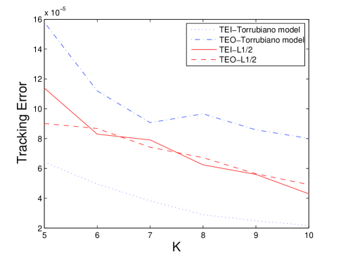
Figure 1: Comparsion of Torrubiano model and $L_{1}/2$ model based on FISE index

$\bullet~{}~{}$ Our model is more stable than Torrubiano’s model since the consistence indicator $Cons2$ is smaller than $Cons1.$

B. Comparison with $L_{1}$ model

Next we conduct experiments to compare the performance of our model using hybrid half thresholding algorithm and $L_{1}$ model using hybrid LARS algorithm. Numerical results are listed in Table 2 and Figure 2.

Table 2: Comparison $L_{1}$ model with our model

Index	Scale	Our model			L1 model			$SupO(\%)$
	$K$	$TEI2$	$TEO2$	$Cons2$	$TEI1$	$TEO1$	$Cons1$
Hang	5	5.81e-5	4.19e-5	1.62e-5	9.65e-5	9.35e-5	2.96e-6	55.15
Seng	6	5.01e-5	3.85e-5	1.16e-5	5.47e-5	7.09e-5	1.62e-5	45.73
$N$=31	7	3.56e-5	2.62e-5	9.38e-6	4.74e-5	5.64e-5	9.06e-6	53.50
	8	2.61e-5	2.02e-5	5.92e-6	4.59e-5	5.95e-5	1.36e-5	66.05
	9	2.31e-5	1.63e-5	6.77e-6	4.41e-5	5.13e-5	7.13e-6	68.20
	10	1.84e-5	1.64e-5	2.07e-6	4.02e-5	4.20e-5	1.79e-6	61.01
DAX	5	4.57e-5	1.20e-4	7.40e-5	3.26e-5	1.22e-4	8.94e-5	1.86
$N$=85	6	3.30e-5	8.78e-5	5.47e-5	2.25e-5	9.89e-5	7.64e-5	11.24
	7	2.41e-5	9.80e-5	7.39e-5	1.66e-5	8.57e-5	6.90e-5	-14.37
	8	2.14e-5	8.97e-5	6.83e-5	1.60e-5	8.04e-5	6.44e-5	-11.48
	9	1.94e-5	8.80e-5	6.86e-5	1.49e-5	7.81e-5	6.32e-5	-12.62
	10	2.96e-5	2.90e-5	5.68e-5	1.43e-5	7.81e-5	6.37e-5	62.82
FTSE	5	1.14e-4	9.01e-5	2.37e-5	1.06e-5	1.33e-4	2.67e-5	32.29
$N$=89	6	8.30e-5	8.68e-5	3.72e-6	9.94e-5	1.18e-4	1.83e-5	26.31
	7	7.91e-5	7.42e-5	4.87e-6	8.78e-5	1.14e-4	2.57e-5	34.63
	8	6.24e-5	6.72e-5	4.83e-6	7.61e-5	1.16e-4	4.02e-5	42.19
	9	5.60e-5	5.64e-5	6.19e-6	5.62e-5	9.40e-5	3.41e-5	39.95
	10	4.30e-5	4.92e-5	6.19e-6	5.34e-5	8.75e-5	3.41e-5	43.74
S&P	5	1.21e-4	1.09e-4	1.06e-5	1.01e-4	1.26e-4	2.44e-5	12.39
$N$=98	6	6.80e-5	8.30e-5	1.50e-5	8.15e-5	9.26e-4	1.10e-5	10.36
	7	8.72e-5	8.33e-5	3.88e-6	5.56e-5	7.51e-5	1.95e-5	-10.95
	8	3.89e-5	5.98e-5	2.08e-5	4.44e-5	6.80e-5	2.36e-5	12.13
	9	7.42e-5	4.90e-5	2.52e-5	4.27e-5	5.98e-5	1.71e-5	18.00
	10	3.99e-5	4.22e-5	2.25e-6	4.22e-5	5.73e-5	1.51e-5	26.39
Nikkei	5	1.26e-4	1.58e-4	3.19e-5	1.48e-5	2.10e-4	6.24e-5	24.72
$N$=225	6	1.15e-4	1.41e-4	2.58e-5	1.31e-5	2.20-4	8.93e-5	35.87
	7	8.81e-5	1.21e-4	3.38e-5	1.18e-5	1.82e-4	6.39e-5	32.85
	8	5.94e-5	9.34e-5	3.40e-5	1.08e-5	1.66e-4	5.83e-5	43.69
	9	5.96e-5	8.14e-5	2.18e-5	9.89e-5	1.62e-4	6.29e-5	49.92
	10	7.08e-5	6.96e-5	1.29e-6	9.47e-5	1.59e-4	6.42e-5	56.25

From the Table 2 we see that our model has lower out-of-sample prediction error than $L_{1}$ model since $SupO>0$ at $87\%(=26/30)$. Moreover, we find our model can provide more sparse solution to track the object index. The Figure 2 shows this results. The out-of-sample prediction error of $L_{1}$ model using $K=10$ stocks is the same to our model using $K=5$ stocks.

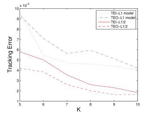
Figure 2: Comparsion of $L_{1}$ model and $L_{1}/2$ model based on Hang Seng index

Finally, we discuss the large scale index tracking problem, i.e., Standard and Poor’s 500($N=457$), Russell 2000 ($N=1318$) and Russell 3000($N=2151$). Since the number of stocks included in indexes is very large, we select the number of the tracking stocks $K=10,20,30,40,50$, the numerical results are listed in Table 3. According to the Table 3, the value $SupO>0$ for all cases, it is shown that our model has better out-of-sample prediction error than $L_{1}$ model.

Table 3: Comparison $L_{1}$ model with our model

Index	Scale	Our model			L1 model			$SupO(\%)$
	$K$	$TEI2$	$TEO2$	$Cons2$	$TEI1$	$TEO1$	$Cons1$
S&P	10	1.49e-4	4.70e-4	2.92e-4	1.08e-4	3.44e-4	2.36e-4	26.88
	20	7.93e-5	2.76e-4	1.97e-4	3.27e-5	1.73e-4	1.41e-4	37.18
$N$=457	30	5.03e-5	2.23e-4	1.72e-4	3.78e-5	1.61e-4	1.23e-4	27.69
	40	3.42e-5	1.68e-4	1.34e-4	3.81e-5	1.10e-4	7.17e-5	34.78
	50	2.57e-5	1.42e-4	1.16e-4	4.18e-5	1.14e-4	7.27e-5	19.17
Russell	10	4.62e-4	5.98e-4	1.37e-4	2.29e-4	5.77e-4	3.48e-4	3.52
$N$=1318	20	1.56e-4	4.34e-4	2.78e-4	1.20e-4	3.83e-4	2.63e-4	11.86
	30	1.06e-4	4.08e-4	3.03e-4	1.30e-4	3.23e-4	1.93e-4	20.94
	40	5.48e-5	3.20e-4	2.66e-4	7.89e-5	2.32e-4	1.53e-4	27.68
	50	5.22e-5	2.89e-4	2.36e-4	9.78e-5	2.62e-4	1.65e-4	9.06
Russell	10	1.26e-4	4.91e-4	3.65e-4	3.78e-4	3.97e-4	1.94e-5	19.14
$N$=2151	20	7.44e-5	3.09e-4	2.34e-4	1.22e-4	2.37e-4	1.15e-4	23.26
	30	3.88e-5	2.37e-4	1.98e-4	1.27e-4	2.28e-4	1.00e-4	3.96
	40	3.39e-5	2.07e-4	1.73e-4	8.45e-5	1.06e-4	1.22e-4	0.44
	50	3.71e-5	1.69e-4	1.32e-4	1.31e-4	1.67e-4	3.56e-5	1.44

5 Conclusions

Index tracking is a passive financial strategy that aims at replicating the performance and risk-profile of a given index. One of the most common approaches to tackle the index tracking problem consists of minimizing a given tracking error measure while limiting the maximum number of assets held in the portfolio. Having few active positions reduces the administrative and transaction costs and avoids detaining very small and illiquid positions, especially when the index has a large number of constituents. However, imposing an upper bound on the number of constituents of the tracking portfolio makes the optimization problem NP-Hard. Different quantitative approaches have been proposed to tackle such an optimization problem. Most approaches rely on search heuristics. On the other hand, $L_{1}$ regularization methods have found application in mean-variance portfolio settings in order to promote the identification of sparse portfolios with good out-of-sample properties and low turnover. However, the $L_{1}$ regularization approach is ineffective in index tracking problem, since the index tracking problem has budget and no-short selling constraints.

In this paper We have used a new constrains $\|w\|_{1/2}^{1/2}=K$ of tracking portfolio’s weight to replace the cardinality constrains $\|w\|_{0}=K$ which equals to $\sum_{i=1}^{N}Z_{i}=K,~{}Z_{i}=0~{}or~{}1$. A new sparse index tracking model was established by minimizing tracking error. Different to the other models of stock index tracking, our model has high consistency and out-of-sample prediction error, it also can preserve sparsity of the optimal tracking portfolio as much as possible. Meanwhile, since the half threshoding algorithm is the fast solver of $L_{1/2}$ regularization, we have extended the half threshoding algorithm to hybrid half thresholding algorithm for solving the proposed index tracking model. The algorithm is fast and efficient with appropriate parameters selection for the sparse index tracking model. Furthermore, it is simple, very convenient in use, and can be applied to large scale problems.

We have tested performance of our model and algorithm on the eight data sets from OR-library. Numerical results have shown that the sparse index tracking model and hybrid half thresholding algorithm have high consisitency and better out-of-sample prediction ability. We believe the sparse index tracking model and projected half thresholding algorithm can provide useful reference to the manager of index derivatives. Next we plan to extend our results to the index tracking problems with transaction costs.

References

- [1] C. Alexander, Optimal hedging using cointegration. Philosophical Transactions of the Royal Society of London, Series A. Mathematical, Physical and Engineering Sciences, 357 (1999), pp. 2039-2058.
- [2] M. Ammann and H. Zimmermann, Tracking error and tactical asset allocation, Financial Analysts Journal, 57 (2001), pp. 32-43.
- [3] J. E. Beasley, OR-Library: Distributing test problems by electronic mail, Journal of the Operational Research Society, 41 (1990), pp. 1069-1072.
- [4] J. E. Beasley, N. Meade and T. J. Chang, An evolutionary heuristic for the index tracking problem, European Journal of Operational Research, 148 (2003), pp. 621-643.
- [5] J. Brodie, I. Daubechies, C. DeMol, D. Giannone and D. Loris, Sparse and stable markowitz portfolios, (2008), ECB Working Paper Series.
- [6] I. R. C. Buckley andR. Korn, Optimal index tracking under transaction costs and impulse control, International Journal of Theoretical and Applied Finance, 1 (1998), pp. 315-330.
- [7] N. A. Canakgoz and J. E. Beasley, Mixed-integer programming approaches for index tracking and enhanced indexation, European Journal of Operational Research, 196 (2008), pp. 384-399.
- [8] E. Candes and B. Recht, Exact matrix completion via convex optimization, Foundations of Computation Mathematics, 9 (2008), pp. 717-772.
- [9] E. Candes and P. Randall, Highly robust error correction by convex programming, IEEE Transactions on Information Theory, 54 (2006), pp. 2829-2840.
- [10] E. Candes and J. Romberg, Quantitative robust uncertainty principles and optimally sparse decompositions, Foundations of Computation Mathematics, 6 (2006), pp. 227-254.
- [11] E. Candes, J. Romberg and T. Tao, Stable signal recovery from incomplete and inaccurate measurements, Communications on Pure Applied Mathematics, 59 (2006), pp. 1207-1223.
- [12] S. S. Chen, D. L. Donoho and M. A. Saunders, Atomic decomposition by basis pursuit,. SIAM Journal of Scientific Computing, 20 (1998), pp. 33-61.
- [13] V. DeMiguel, L. Garlappi, J. Nogales and R. Uppal, A generalized approach to portfolio optimization: Improving performance by constraining portfolio norms, 2008, Working Paper.
- [14] D. L. Donoho, Compressed sensing, IEEE Transactions on Information Theory, 52 (2006), pp. 1289-1306.
- [15] B. Efron, T. Hastie, I. Johnstone and R. Tibshirani, Least angle regression, Annals of Statistics, 23 (2004), pp. 407-499.
- [16] Jianqing Fan, Jingjin Zhang and Ke Yu, Asset allocation and risk assessment with gross exposure constraints for vast portfolios, 2008, Working paper.
- [17] R. Fernholz, R. Garvy and J. Hannon, Diversity weighted indexing, Journal of Portfolio Management, 24 (1998), pp. 83-92.
- [18] M. Gilli and E. Kellezi, Threshold accepting for index tracking, Working paper available from the first author at Department of Econometrics, University of Geneva, 1211 Geneva4, 2001, Switzerland.
- [19] A. E. Hoerl and R. W. Kennard, Ridge regression: Biased estimation for nonorthogonal problems, Technometrics, 8 (1970), pp. 27-51.
- [20] R. Jagannathan and T. Ma, Risk reduction in large portfolios:why imposing the wrong constraints helps, Journal of Finance, 58 (2003), pp. 1651-1683.
- [21] Y. Karklin and M. S. Lewicki, Emergence of complex cell properties by learning to generalize in natural scenes, Nature, 457 (2009), pp. 83-86.
- [22] M. Lobo, M. Fazel and S. Boyd, Portfolio optimization with linear and fixed transaction costs, Annals of Operations Research, 152 (2007), pp. 341-365.
- [23] N. Meinshausen and P. Buhlmann, High dimensional graphs and variable selection with the lasso, Annals of Statistics, 34 (2006), pp. 1436-1462.
- [24] B. A. Olshausen and D. J. Field, Emergence of simple-cell receptive field properties by learning a sparse code for natural images, Nature, 381 (1996), pp. 607-609.
- [25] R. A. Roll, Mean-variance analysis of tracking error, The Journal of Portfolio Management, 18 (1992), pp. 13-22.
- [26] M. Rudolf, H. J. Wolter and H. Zimmermann, A Linear model for tracking error minimization, Journal of Banking and Finance, 23 (1999), pp. 85-103.
- [27] J. Shapcott, Index tracking: genetic algorithms for investment portfolio selection (Technical report, EPCC-SS92-24), Edinburgh, Parallel Computing Centre, 1992.
- [28] Q. Sun, B. Gao, L. Jian and C. Y. Wang, Modified conjugate gradient projection method for nonlinear constrained optimization, Acta mathematicae applicatae sinica, 2010, pp. 4640-651.
- [29] Y. Tabata and E. Takeda, Bicriteria optimization problem of designing and index fund, Journal of the Operational Research Society, 46 (1995), pp. 1023-1032.
- [30] P. R. Torrubiano and S. Alberto, A hybrid optimization approach to index tracking, Annals of Operation Research, 166 (2009), pp. 57-71.
- [31] R. Tibshirani, Regression shrinkage and selection via the lasso, Journal of the Royal Statistical Society, 46 (1996), pp. 431-439.
- [32] Z. B. Xu, H. L. Guo, Wang Y. Wang, The representation of L1/2 regularizer among Lq regularizer: an experimental study based on phase diagram. Acta Autom Sin, 2011 (in press).
- [33] Z. B. Xu, H. Zhang, Y. Wang and X. Y. Chang, L1/2 regularization, Science in China (series F), 40 (2010), pp. 1-11.
- [34] Z. B. Xu, X. Y. Chang, F. M. Xu and H. Z hang, L1/2 regularization: an iterative half thresholding algorithm, IEEE Transactions on neural networks and learning systems, 23 (2012), pp. 1013-1027.