Towards the azimuthal characteristics of ionospheric and seismic effects of ”Chelyabinsk” meteorite fall according to the data from coherent radar, GPS and seismic networks
Abstract
We present the results of a study of the azimuthal characteristics of ionospheric and seismic effects of the meteorite ’Chelyabinsk’, based on the data from the network of GPS receivers, coherent decameter radar EKB SuperDARN and network of seismic stations, located near the meteorite fall trajectory. It is shown, that 6-14 minutes after the bolide explosion, GPS network observed the cone-shaped wavefront of TIDs that is interpreted as a ballistic acoustic wave. The typical TIDs propagation velocity were observed , which corresponds to the expected acoustic wave speed for 240km height.
14 minutes after the bolide explosion, at distances of 200km we observed the emergence and propagation of a TID with spherical wavefront, that is interpreted as gravitational mode of internal acoustic waves. The propagation velocity of this TID was which corresponds to the propagation velocity of these waves in similar situations. At EKB SuperDARN radar, we observed TIDs in the sector of azimuthal angles close to the perpendicular to the meteorite trajectory. The observed TID velocity (400 m/s) and azimuthal properties correlate well with the model of ballistic wave propagating at 120-140km altitude.
It is shown, that the azimuthal distribution of the amplitude of vertical seismic oscillations can be described qualitatively by the model of vertical strike-slip rupture, propagating at 1km/s along the meteorite fall trajectory to distance of about 40km. These parameters correspond to the direction and velocity of propagation of the ballistic wave peak by the ground.
It is shown, that the model of ballistic wave caused by supersonic motion and burning of the meteorite in the upper atmosphere can satisfactorily explain the various azimuthal ionospheric effects, observed by the coherent decameter radar EKB SuperDARN, GPS-receivers network, as well as the azimuthal characteristics of seismic waves at large distances.
1 Introduction
The bolide, observed on February, 15 2013 above Chelyabinsk region, Russia, is the second powerful event since the fall of the Tunguska meteorite in 1908 [Zotkin and Tsikulin1966, Ben-Menahem1975]. According to [Popova et al.2013], ’Chelyabinsk’ meteorite had an initial size of about 19.8 meters and an initial weight of about 13000 tons. When entering the atmosphere, its velocity was about 18.6 km/s. The most powerful explosion (the main explosive disruption) occurred at 03:20:32UT (09:20:32LT) at height. After that, two more explosions occurred: second disruption (03:20:33.4UT) and third disruption (03:20:34.7UT) [Popova et al.2013].The energy of its burning in the atmosphere, that caused the destruction of buildings and windows, according to the calculations of [Popova et al.2013] was equivalent to 590 kilotons (kT) of TNT, while the part of the energy, associated with explosions, looks relatively small [Popova et al.2013] (see support materials(SM), pp.62-69 in [Popova et al.2013]). The paper [Alpatov et al.2013] has shown, that the kinetic energy of the explosion of the ’Chelyabinsk’ meteorite was based on the data of 11 infrasound stations of International Monitoring System of nuclear tests (MSM).
Midscale travelling ionospheric disturbances (MSTIDs) with few hundred kilometers spatial scale, and few tens of minutes temporal scale, that were caused by the flight and explosion of the ’Chelyabinsk’ meteorite, were detected by various instruments [Alpatov et al.2013, Givishvili et al.2013, Gokhberg et al.2013, Berngardt et al.2013a, Yang et al.2014, Ruzhin et al.2014, Chernogor2015].
By using low-orbital tomography at vertical ionospheric profiles over the European territory of Russia, wave-like disturbances (wavelength at latitude) were detected, that appear 2.5-3 hours after the explosion [Alpatov et al.2013, Givishvili et al.2013]. The disturbances of the total electron content (TEC), caused by the explosion, were detected by ARTU GPS station [Gokhberg et al.2013, Ruzhin et al.2014, Chernogor2015]. According to [Gokhberg et al.2013] TEC variations had an inverted N-wave shape. The distribution of TEC variations amplitudes was not spherically symmetric. The ionospheric response to the explosion had a number of features (waveform, axial symmetry in the ionospheric disturbances distribution) distinguishing it from the ionospheric response to earthquakes, tsunamis, explosions and volcanic eruptions [Gokhberg et al.2013].
In [Yang et al.2014], using GPS networks near the meteorite trajectory, in Japan and in the United States, three different types of MSTIDs were found: the higher-frequency (4.0-7.8mHz, periods 4.2-2.1min) disturbances were observed around ARTU station and having velocity; the lower frequency (1.0-2.5mHz, periods 16.7-6.7min) disturbances, propagating with a mean velocity , were observed at distances of 300-1500km from Chelyabinsk; the higher-frequency (2.7-11mHz, periods 1.5-6.2min) disturbances with a mean propagation velocity were registered in USA region. Within 14min after the bolide explosion, on several nearby GPS-stations different TEC variations were observed: some of them were caused by solar terminator and some of them propagate radially from the explosion epicenter to the distances up to 500-600km with 320-360m/s velocity [Berngardt et al.2013a]. At 06:00-10:00UT at most GPS stations, located away from the meteorite trajectory, an intensive TEC variations were observed, which had the form of wave packets with 30-40min period [Berngardt et al.2013a].
According to the over-the-horizon coherent EKB SuperDARN radar, located 200 km from the meteorite explosion place, it is shown that the flight and fall of the meteorite caused the formation of MSTIDs with 150-200km horizontal spatial scale, propagating throughout the entire ionosphere (in E- and F-layers) to the distances up to 1500km from the epicenter. They have two typical propagation velocities - 220m/s and 400m/s [Berngardt et al.2013b].
This paper presents the results of studying the azimuthal features of MSTIDs and seismic effects of ”Chelyabinsk” meteorite according to GPS network, EKB SuperDARN radar and network of seismic stations, located near the meteorite trajectory.
2 Observations
2.1 GPS TEC variations
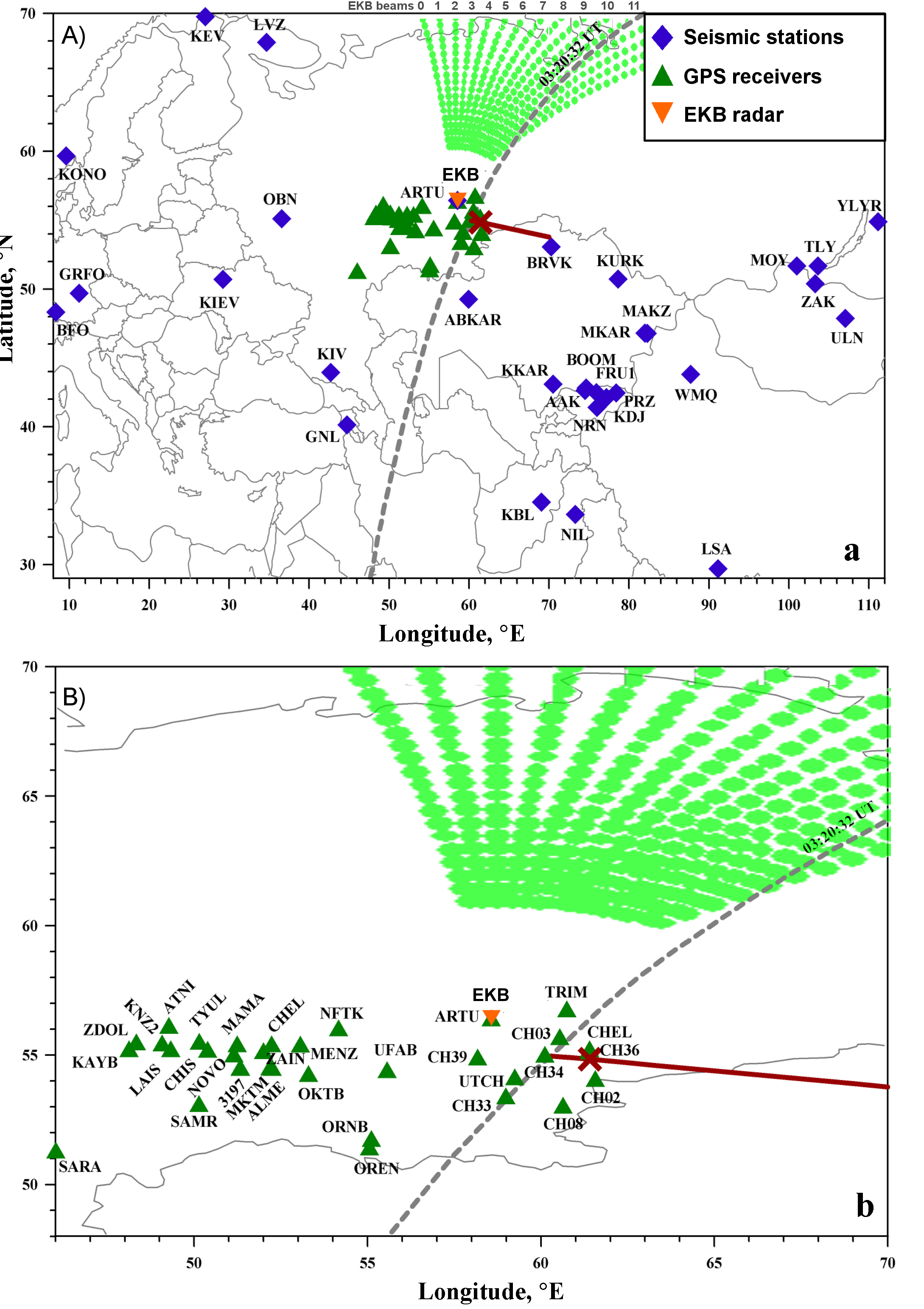
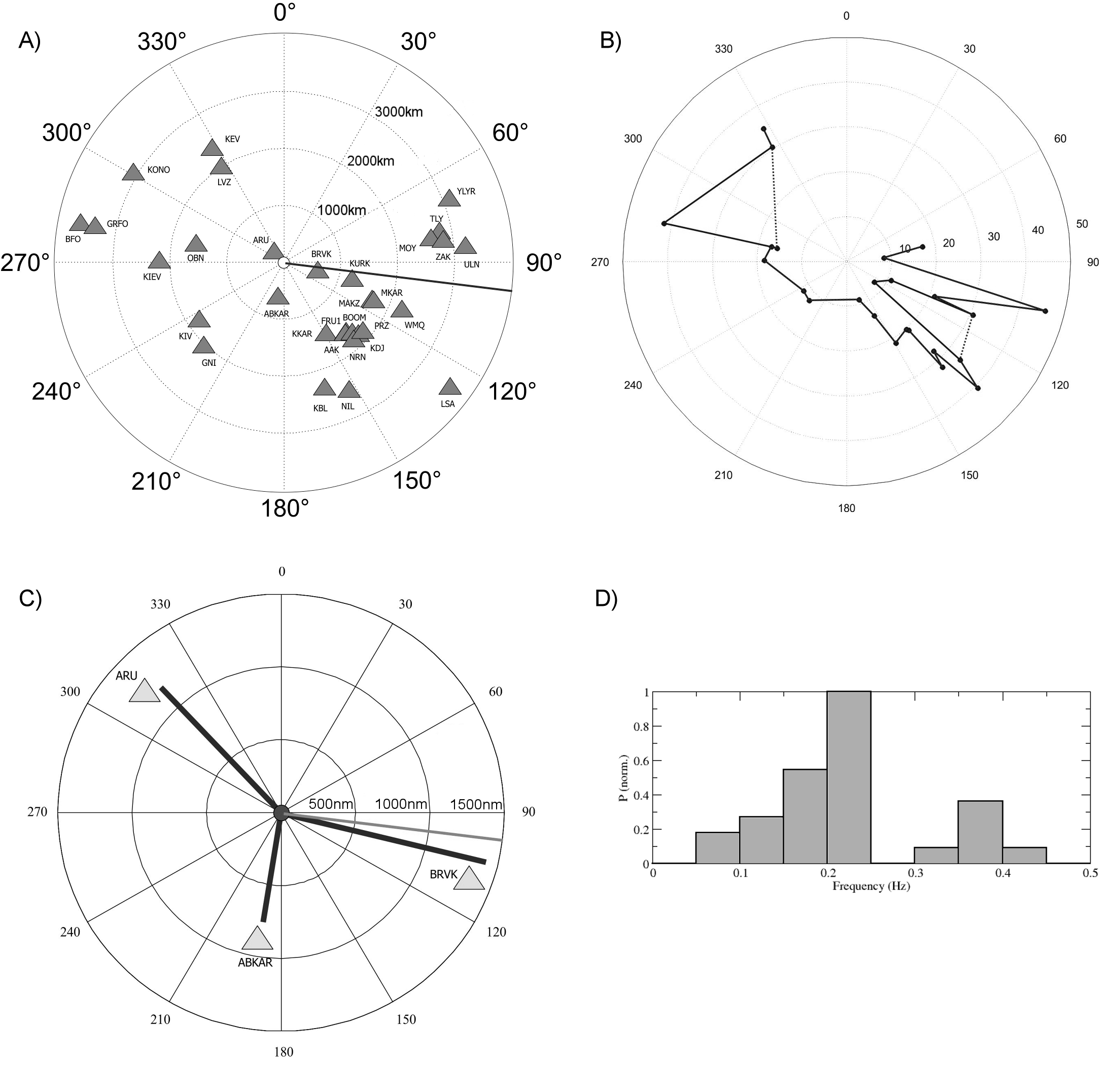
The study of TEC variations in the ionosphere during Chelyabinsk meteoroid flight was based on phase measurements of double-frequency GPS receivers (Fig.1). The data (with 1-sec sampling rate) of ARTU GPS-station included in the International GNSS Service (IGS) network were downloaded from the Scripps Orbit and Permanent Array Center website (http://sopac.ucsd.edu). GPS data (with 30-sec sampling rate) of stations TRIM and ORNB operated by NAVGEOKOM company were available from http://www.navgeocom.ru. Data of GPS receivers in the Chelyabinsk region (CHEL, CH02, CH03, CH08, CH33, CH34, CH36, CH39; 5-sec sampling rate) were kindly provided by LLC ”GEOSalyut” (Moscow) and LLC ”Poleos” (Chelyabinsk). The Kazan GPS network data (stations LME, ATNI, CHEL, CHIS, KAYB, KZN2, LAIS, MAMA, MENZ, MKTM, NFTK, NOVO, OKTB, OREN, SAMR, SARA, TYUL, UFAB, UTCH, ZAIN, ZDOL, 30-sec sampling rate; stations 3192, 3196, 3197, 3199, 3204, 15-sec sampling rate) were provided by Federal Kazan University (KFU) and RPC ”Geopoligon” KFU (Kazan). The last five GPS-stations are very close to each other and shown as single 3197 station at Fig.1.
The area around F2-layer maximum (height ) make the main contribution to TEC variations. Therefore, it is assumed that TEC variations are formed in an ionospheric piercing point (IPP), where IPP is the point of intersection of the ”receiver-satellite” line of sight (LOS) with an ionospheric layer at . According to ARTI ionosonde, located in Ekaterinburg, during meteorite fall was about 243 km. We used this value in our calculations.
To separate disturbances triggered by the meteoroid explosion, the initial TEC series I(t) were converted to an equivalent ”vertical” value [Klobuchar1986], and then we filtered it in the period range 1-20 min [Afraimovich et al.1998]. TEC variations occurring on the day of the meteorite fall were compared with the TEC behavior observed on previous and subsequent days. The analyzed period featured quiet geomagnetic conditions: Kp-index did not exceed 1 within 00:00-12:00 UT, and there were no strong solar flares. The seismic background was also quiet in the Chelyabinsk region and nearby areas. Some difficulties in separating the meteorite-generated ionospheric disturbances were caused by the fact that the meteoric impact occurred at sunrise, when the ionosphere exhibited strong variability. [Afraimovich et al.2009] demonstrated that solar terminator (ST) generates TEC wave disturbances in the ionosphere. Such disturbances can be seen for 2-4 h and even precede ST, which is attributed to the ST passage through the magnetoconjugate region. Between 02:00 and 06:00 UT on February 14-16, 2013, almost in all LOSs in the TEC variations there were quite intense oscillations with an amplitude of 0.2 TECU and a period of 15-17 min. It is most likely that they were caused by the ST passage.
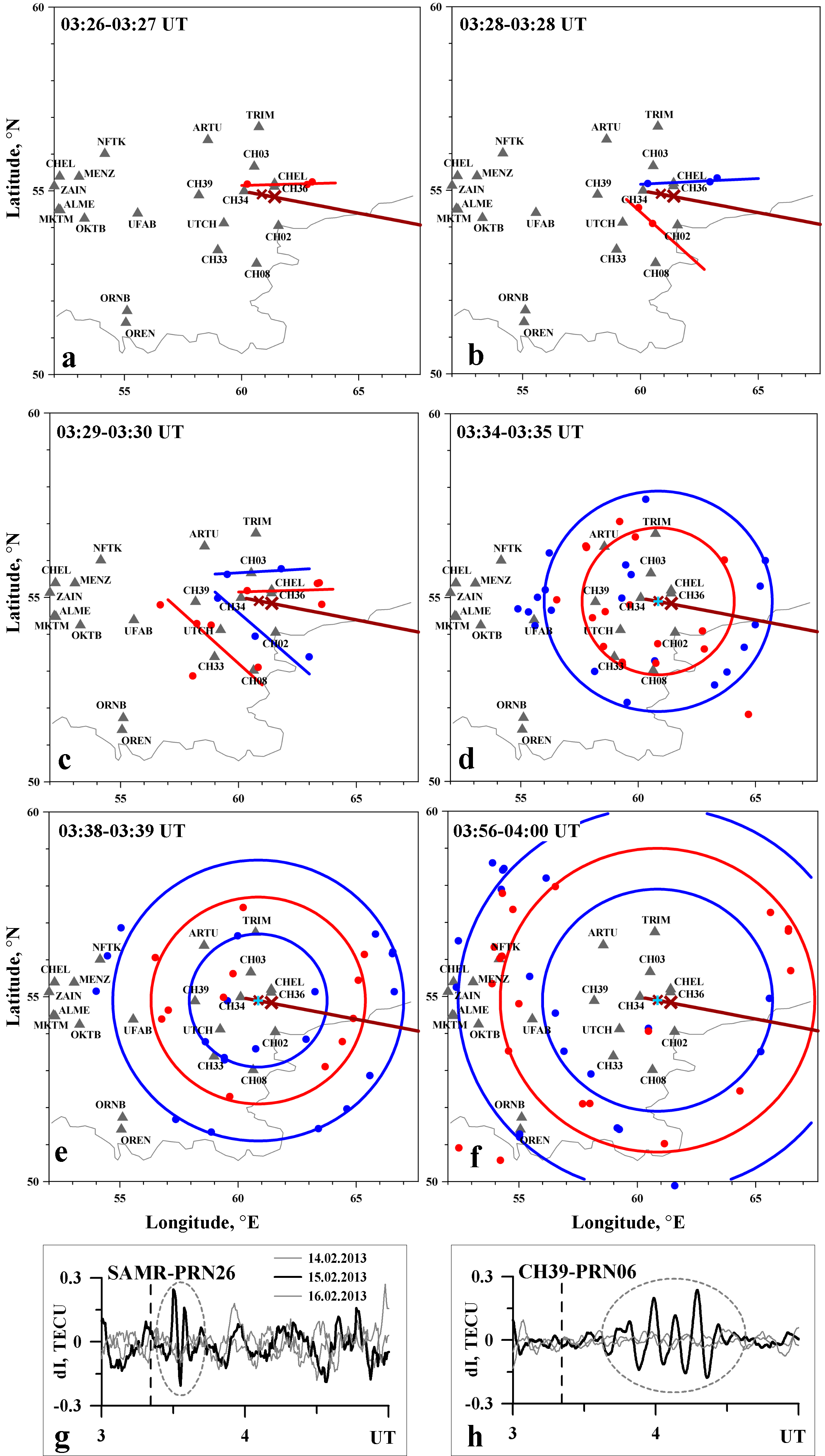
Nevertheless, in spite of the presence of ST-caused TEC oscillations, in some receiver-satellite LOSs we managed to separate disturbances with a characteristic shape corresponding to the shape of a shock acoustic wave. In Fig.2g-h, such disturbances are marked with dashed lines. These disturbances were oscillations with a period of min and amplitude 0.07-0.5 TECU exceeding the level of background oscillations on the reference days.
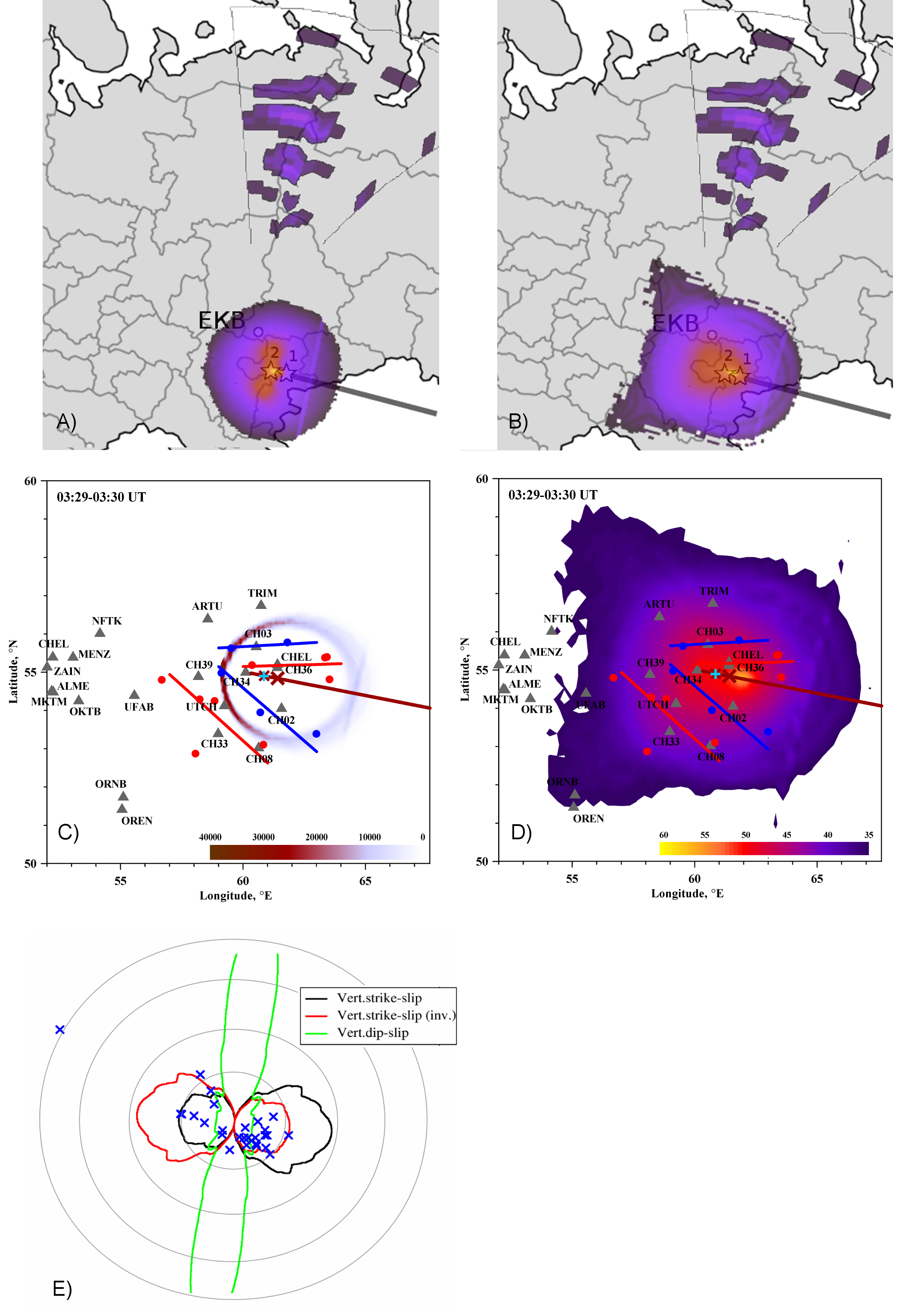
To draw a spatial-temporal picture of the TEC response to the meteoroid explosion, we have constructed TEC disturbance maps (Fig.2a-f). Figure 2a-f presents spatial distribution of minima (blue dots) and maxima (red dots) of TEC oscillations (at ) over a period 03:26-04:00 UT. Thick concentric lines indicate the position of the disturbance wave front which can be traced through TEC variations minima (blue) and maxima (red). The first TEC disturbances were registered 6 min after the meteorite explosion at distances of 80-100 km from the airburst location. Over a period 03:26-03:33 UT, the TEC disturbances are characterized by fast dynamics. The front of disturbances has a form of the cone dispersing from the meteorite trajectory. The angle at a cone peak changes from to (the average angle value is about ). The average velocity was estimated from movement of front lines: . Since 03:34 UT the behavior of the TEC disturbances corresponds to the spherical wave front propagating from the center with coordinates (blue cross in Fig.2d-f). The wave center is shifted approximately 37 km northwestward of the airburst. It coincides with the location of meteorite tertiary disruption () [Popova et al.2013]. The analysis suggests that the TEC disturbances propagated radially up to 600-700 km and had wavelength around 220 km. The average velocity calculated from movement of front lines was . It should be noted that spherical wave is generally registered eastward, northeastward, and southeastward from the airburst. The interference of two wave types (spherical and cone-shaped) is observed westward, northwestward, and southwestward from the airburst. This effect is more expressed during 03:34-03:38 UT.
2.2 Coherent radar observations
Measurements by GPS network are known to have difficulty in separating the spatial and temporal variation of ionospheric parameters. Unlike GPS data, SuperDARN radars [Chisham et al2007] have high spatial and temporal resolution, and allows us to differ spatial and temporal effects. The first Russian coherent radar EKB is located (near Ekaterinburg city), approximately 200 km to the North-West from the meteorite fall region and operated with 60km spatial and 1min temporal resolution in the sector from North at distances up to 3500km. Fig.1 shows the location of the radar and the orientation of each of the 16 rays (beams) of its field of view.
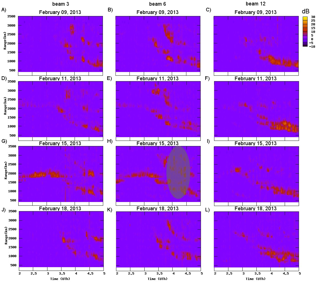
After the meteorite fall, EKB radar recorded a large variety of ionospheric effects [Berngardt et al.2013a, Berngardt et al.2013b, Berngardt2013c, Kutelev and Berngardt2013]. The most powerful and basic effect is the observations of formation and radial passage of MSTIDs at E- and F-layer heights [Kutelev and Berngardt2013]. Fig.3 presents the power of the scattered signal according to EKB radar data at 3,6,9,12 beams (Fig.3I-L) during February 15, 2013 02:00-05:00UT. In addition, the figure shows the power of the scattered signal in geomagnetically quiet days - February 09, 11, 18, 2013. The choice of these days been investigated in detail, for example, in [Kutelev and Berngardt2013].
The tracks marked by areas 1-2 in the figure correspond to refraction of the radiosignal at ionospheric irregularities, which propagate radially from the radar with velocities 400 and 200 m/s at E- and F-layer altitudes [Kutelev and Berngardt2013].
According to Fig.3, the ionospheric effects in the field of view of the radar have strong azimuthal dependence. In particular, they present on 6 beam, and do not appear at 3 and 12 beams. To emphasize the azimuthal effects, we used the following technique:
- For each moment, for each beam, and for each range (this allows us to uniquely define each region in the field of view with approximately 100x100km size) we calculate the average power (in dB) higher than the noise level 0dB, over the magnetically quiet days February, 09,11,18, 2013;
- Then, when processing 02/15/2013 data for each moment, beam and range we analyse only the data exceeding the threshold level (tripled the calculated average power at this point).
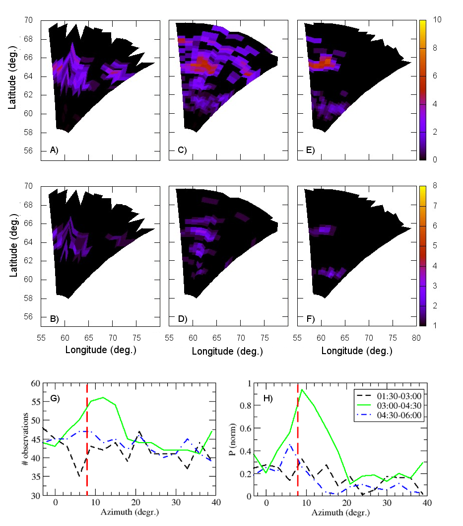
- The power and the number of observations, accumulated for the given time period for every fixed beam and every fixed range, are shown in Fig.4.
Fig.4A,C,E shows the intensity of the scattered signals in the radar field of view above the threshold level. Fig.4B,D,F presents the number of signals exceeding a threshold level.
As one can see from Fig.4C-D, the main effect is concentrated in the sector of directions from the north. The dotted line marks the direction corresponding to the perpendicular to the meteorite trajectory.
2.3 Seismic observations
For the analysis of the seismic characteristics, we used seismograms obtained by worldwide networks of the broadband seismic stations Iris/Ida (II, http://ida.ucsd.edu/) and Iris/USGS (IU, http://earthquake.usgs.gov/regional/asl/) and by four regional networks: Iris/China (IC), Kazakhstan (KZ), Kyrgyzstan (KR) and Baikal regional seismological center (BY, Russia). Analysis of seismograms is a bit complicated due to presence of seismic waves from Tonga earthquake (February 15, 2013, 03:02:23UT, magnitude 5.8, coordinates 19.72S, 174.48W, depth 71.6 km). In the rest, the seismic situation was very quiet - no local or regional earthquakes were registered on the seismograms. Visual analysis revealed the presence of the surface seismic waves at some stations that may be associated with meteorite according to their arrival times. These waves were recorded at 32 seismic stations (Fig.5A), located at distances from 252 to 3654 km from the epicenter, and they are short-period oscillations with a period T = 3-16 sec and with duration up to 1 minute. For stations situated more than 3600 km from the fall site, a surface wave is lost in the seismic waves from the Tonga earthquake. The group velocity of Rayleigh waves for periods of 20-100 seconds varies from 2.3 to 3.5 km/s.
For the analysis of azimuthal distribution of surface seismic waves the maximal amplitudes of vertical oscillations (Fig.5B), and the spectral corner frequencies were analyzed (Fig.5D). The distribution of seismic stations around the point of the explosion is non-uniform: there is a very big azimuthal gap approximately from to . For this azimuthal range it is impossible to allocate the surface wave from the records due to the superposition of waves from the Tonga earthquake, as well as to the lack of broadband seismic stations ( Fig.5A). Analysis of at the nearest stations ( 620 km) shows that the maximum = 1414.4 nm is observed at station BRVK (= 616 km, azimuth - ), at the same time, the amplitude at station closer to the fall point is smaller: at ARU station ( = 252 km, azimuth ) =1177.5 nm, at ABKAR station ( = 618 km, azimuth ) - = 762.4 nm (Fig.5C).
The azimuthal distribution of the maximum amplitudes of the Rayleigh waves at different stations indicates the absence of spherical symmetry (Fig.5B) - the maximum amplitudes are oriented along the direction of the meteorite trajectory, the minimum amplitudes are observed in perpendicular directions. There is three exceptions: an abnormally low amplitudes are observed at LSA (distance = 3654 km) and MKAR ( = 1709 km) stations, located in azimuths , and abnormally high amplitude at the KONO station (azimuth , = 3073 km). But statistically, the azimuthal distribution of the Rayleigh waves amplitudes has two peaks elongated with the meteorite trajectory: the first maximum is oriented towards the meteorite fall direction and the second - in the opposite direction.
The analysis of the azimuthal distribution of showed that the distribution elongated with the meteorite fall trajectory (Az = ). At the same time, we found no spherical symmetry in seismic wave radiation that corresponds to bolide explosions. This allows to suggest that the seismic effect is caused by single extended event rather than a series of explosions. This fits well in with the model [Popova et al.2013]. An explanation of the observed asymmetry in the seismic wave amplitudes from the single point source is also not satisfactory. In some cases, azimuthal nonuniformity of the seismic wave amplitudes may be explained by an anisotropy of medium. But this explanation does not work in our case, as the main tectonic structures in the Ural region are oriented orthogonally to the meteorite trajectory. Thus, we can conclude that there is a directivity of seismic radiation.
The effect of directivity is reflected both in the seismic wave amplitudes and on the corner frequencies. The concept of the corner frequency is associated with the rupture parameters (its velocity and length) and directivity function [Ben-Menahem1961]:
| (1) |
where is the seismic wave velocity, is the rupture speed, is the length of rupture, is angular frequency, is the angle between the rupture propagation direction and the direction to the seismic station.
This function has a series of maxima and minima at frequencies, their positions depend on the values and . The first maximum/minimum corresponds to a frequency called the corner frequency. Thus, the corner frequency includes the effect of the propagation of rupture and it may be measured directly from the surface wave spectrum. It corresponds to the frequency of the inflection point of the seismic spectrum, separating the horizontal plateau at low frequencies and decaying oscillations with sloping envelope at high frequencies. For the meteorite surface waves, the corner frequencies vary widely (0.06-0.43 Hz), but the maximum number of stations observe frequencies 0.15 - 0.25 Hz (Fig.5D).
3 Models
3.1 Acoustic signal model
To explain the azimuthal characteristics of ionospheric effects, we made mathematical simulations of acoustic signal propagation at different heights.
Models based on one or more explosions are often considered as model caused by the ionospheric disturbances. However, from our point of view, the model of ballistic wave described in (SM in [Popova et al.2013], pp.62-69) is the most realistic one. It successfully explains the observed destructions (which are associated with a passage of powerful acoustic wave) as continuous formation of perturbations along the meteorite trajectory. Similar models have been successfully used for explaining the zone of destruction after the Tunguska meteorite fall [Zotkin and Tsikulin1966, Ben-Menahem1975], which indicate a high degree of this model reliability. In this model, the amplitude of the source along the trajectory is determined by the luminosity of the bolide [Zotkin and Tsikulin1966]. The disadvantages of using other models to describe the destruction zone in the case of ’Chelyabinsk’ meteorite were investigated in detail in (SM in [Popova et al.2013],pp.62-69).
Therefore, we used the simple model of the summation of partial pressures coming from each point of the meteorite trajectory with taking into account the acoustic propagation delay. We used the model of a moving source. The initial acoustic pressure disturbance is proportional to the luminosity of the bolide at the meteorite position for given moment [Zotkin and Tsikulin1966, Ben-Menahem1975]. The luminosity is shown in (SM in [Popova et al.2013], pp26-27).
As a result of interference, the meteorite fight forms the focus of the acoustic wave - Mach cone (ballistic wave). In a homogeneous medium for the meteorite velocity 17.5km/s this wave spreads nearly perpendicularly to the flight trajectory. In a medium with nonuniform acoustic speed height profile the Mach cone shape substantially transforms. This transformation is determined by many factors, including the acoustic speed at different heights. Therefore at different distances, the angle between propagation direction and the meteorite trajectory becomes different.
For estimates, we used the qualitative model for dependence of the acoustic wave pressure on the neutral density and acoustic speed [Yuen1969]:
| (2) |
Here, the delay is determined by trajectory of the acoustic signal and based on the geometrical optics laws for the acoustical signal in inhomogeneous media [Blokhintsev1952, Clay and Medwin1977], where the refractive index is determined by the acoustic speed . The is the density of the neutral atmosphere and is the initial acoustic pressure of the source, which (in the first approximation) is equal to the luminosity of the bolide at this point at corresponding moment [Zotkin and Tsikulin1966, Ben-Menahem1975] with accuracy of a constant multiplier . is the position of the bolide in the moment .
The resulting partial acoustic pressure at each point of is summed up with taking into account the geometroacoustic propagation delay from the bolide (source) point to the specified point. Since the source of the acoustic wave at each moment is assumed isotropic, we conducted an additional integration over all the acoustic signal propagation directions from the source point.
The duration of the meteorite fall in the upper atmosphere was , which corresponds to a wavelength , considerably less than a hundred kilometers - the distance to the studied effects. This can qualitatively substantiate the applicability of geometrical acoustics for qualitative estimates of the observed ionospheric effects. In the calculations of the acoustic field, we assumed that the acoustic speed and the neutral density profile are functions of the height . The earth surface is considered to be flat, due to the smallness of the investigated distances. The acoustic speed and neutral density profile were estimated from the reference model NRLMSIS-00 for observation point.
As an initial pressure perturbation , forming an acoustic signal we used a short pulse propagating at the velocity along the meteorite trajectory from 90km to 25km altitude. depends on the height and luminosity curve defined in (SM in [Popova et al.2013], pp26-27). We used the data given in [Borovicka et al.2013] for entry point , the trajectory and meteorite fall velocity .
It should be noted that the model is very rough, and does not include neither details of the acoustic signal amplitude changes with height, nor conversion of neutral density variations into electron density variations. The effects also depends on the height [Maruyama and Shinagawa2014] and their presence is required for a correct estimation of the amplitude of ionospheric effects. However, as it will be shown below, the model is suitable for qualitative explanation of azimuthal and temporal effects.
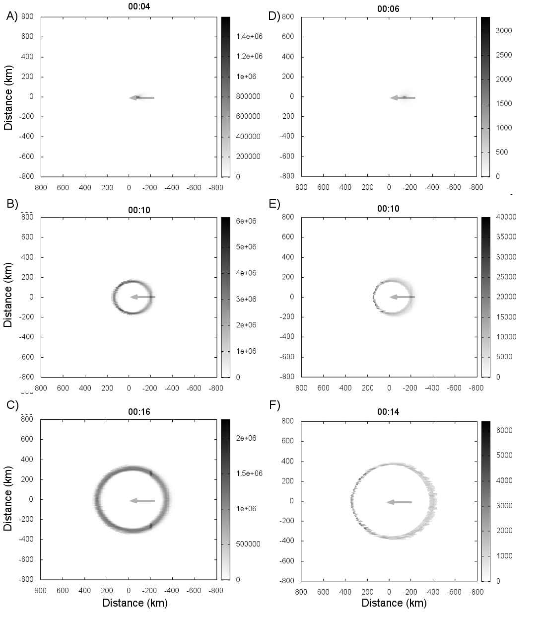
The evolution of amplitude at 120km altitude, in E-layer, as a function of time, is shown at Fig.6a-c. One can see from the figure that the main acoustic effects should be observed 4-6 minutes after the explosion and spread further at the acoustic speed () in a direction perpendicular to the meteorite fall trajectory.
Fig.6d-f presents the evolution of acoustic wave pressure at 240km, in the F-layer, as a function of time. It shows that the main acoustic effects should be observed 7-8 minutes after the explosion and should propagate with acoustic speed () in a direction of to the meteorite trajectory.
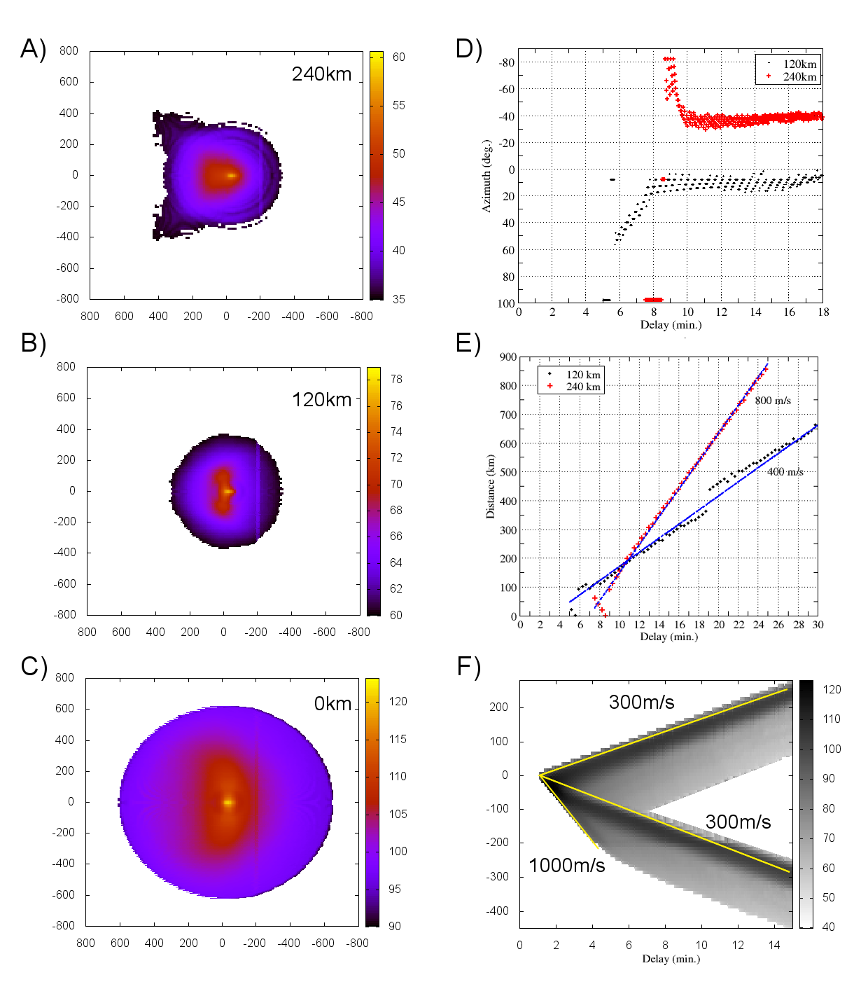
Fig.7a-c shows the modeled acoustic wave maximal pressure at various heights and at various distances from the main bolide explosion site, with taking into account the acoustic sound speed profile at the upper atmosphere.
It can be seen that the acoustic wave pressure at different altitudes has a strong azimuthal dependence. At relatively low altitudes (below 150 km), the highest acoustic wave pressure is predicted at azimuths perpendicular to the meteorite trajectory. This fits well with the results of [Popova et al.2013] which associate the azimuthal features of the destruction zone on the earth’s surface with an acoustic wave pressure. This justifies the possibility of using the simple model (2) for estimation of azimuthal effects. At altitudes above 150 km, the model predicts an increase of the acoustic wave pressure at azimuths to the meteorite trajectory in the direction of the meteorite fall.
From Fig.7A-C one can see that the highest acoustic wave pressure is observed under the trajectory of the meteorite. Fig.7C shows the dynamics of the acoustic wave pressure along the meteorite trajectory projection to the Earth’s surface. As it is shown at Fig.7 F, three acoustic disturbances propagate along the surface of the Earth: the most powerful propagates back towards its fall with velocity, which is defined by the meteorite trajectory fall angle, the meteorite speed and the acoustic speed profile. This velocity roughly coincides with the estimates given in (SM in [Popova et al.2013], p.70), which also confirms the possibility of using our model to estimate the effects. The two other waves are acoustic ones, having velocity , which is associated with the propagation of spherical acoustic wave at ground altitudes.
3.2 Seismic signal model
The propagation velocity of surface seismic waves was about 3-3.5km/s [Tauzin et al.2013]. Therefore the seismic oscillations at longer distances can not be directly caused by atmospheric acoustic waves having the velocity 10 times smaller. However, the movement of a supersonic powerful acoustic pulse (ballistic wave) on the ground can cause the observed seismic effect indirectly. This model, for example, was used for an explanation of seismic effects of Tunguska meteorite [Ben-Menahem1975]. To estimate the characteristics of the effect we carried out numerical calculations of the signal intensity in a simple model developed for the analysis of seismic signals generated during formation of geological faults. As the fault line we use the trajectory of the acoustic signal on the ground. Parameters of fault formation (length, velocity and direction) are equal to the parameters of the acoustic pulse movement on the ground.
To calculate the theoretical seismic radiation pattern we used the model proposed in [Ben-Menahem1961] for a linear fault. According to this approach, the azimuthal distribution of the seismic waves is defined by the type of the fault and by the parameters of its formation: the rupture speed , its length , the frequency of seismic waves , and the phase velocity of Rayleigh waves .
In our case, two types of ruptures with the vertical position of the plane displacement may be considered as a seismic analogue - vertical strike-slip fault and the vertical dip-slip fault. In both cases, the maximal amplitudes have to orient according to the slip vector: for the strike-slip fault – they are oriented in the direction strike fault, and for dip-slip fault – they are perpendicular to the fault plane [Kasahara1981, Udías et al2014].
In our analysis, we used the following formulas that qualitatively describe (up to a constant multiplier) the azimuthal distribution of amplitudes of vertical seismic oscillations in cases of different fault types. Thus, the amplitude of the seismic waves depends strongly on the angle between fault propagation direction and the direction to the seismic station. The amplitude also depends on the distance to the observation point .
According to [Ben-Menahem1961], in the case of vertical strike-slip fault the azimuthal distribution of the Rayleigh displacement for the vertical component is given by:
| (3) |
where
| (4) |
In the case of vertical dip-slip fault the azimuthal distribution of the Rayleigh displacement for the vertical component is given by:
| (5) |
where
| (6) |
For the simulation we choose the propagation line of the fault as the trajectory of the meteorite fall (azimuth of propagation ).
We suppose the rupture speed , its length , the frequency of seismic waves , defined from fig.5D and the phase velocity of Rayleigh waves .
The direction of the rupture was opposite to the direction of the fall. This corresponds to the direction and the trajectory of the ballistic wave peak on the ground.
4 Discussion
Fig.8A,B presents a comparison between observed MSTIDs and acoustic wave pressure distribution at 120km. One can see that the model of acoustic waves in the lower ionosphere describes the experimental data sufficiently well. The same conclusion can be made from a comparison of Fig.7c and Fig.4. According to the estimates carried out before, the velocity of azimuth-dependent ionospheric irregularities was about 400m/s [Kutelev and Berngardt2013]. This corresponds well to the velocity of acoustic wave pressure variations at altitudes 120-140km. So we can conclude that the MSTIDs, observed by EKB radar, are well described by the effect of the ballistic wave passage at altitudes of 120-140km. This also stimulates similar disturbances in the charged components of ionospheric plasma (for example, by mechanism described in [Maruyama and Shinagawa2014]).
As simulations show, the acoustic radiation pattern at 240km has a specific two-horned structure, which describes the experimental results observed in the first 14 minutes after the explosion sufficiently well. Fig.8C-D shows the imposition of model calculations and experimental observations. We can see from Fig.8C that not only irregularities azimuthal distribution, but also the expected moment of irregularities observation are in a good agreement with the model. Estimates of the propagation velocity of TEC wave cone 6-14min after explosion is , and are in a good agreement with the calculated acoustic wave pressure velocity at 240km height (Fig.7 E). The observation of such waves by the EKB radar is hampered by the fact that the azimuthal effect is located outside the antenna pattern.
14 minutes after the explosion we observed a formation and propagation of a spherical MSTID with velocity . Similar midscale (wavelength of 200-300 km) concentric MSTIDs with velocities were detected by GPS receivers after the Tohoku earthquake (March 11, 2011) [Tsugawa et al.2011]. The earthquake-generated MSTIDs began to be observed at distances from the epicenter, and propagated up to 1000km. According to the numerical simulation [Matsumura et al.2011], these propagating spherical MSTIDs can be related with gravitational mode of internal atmospheric waves.
Thus, by GPS network we observed the two MSTID kinds in TEC: the conical wavefronts associated with ballistic wave 6-14 minutes after the explosion, and the spherical wavefronts associated with internal airwave 14 minutes after the explosion.
Fig.8E shows the azimuthal distribution of the amplitude of vertical seismic oscillations, multiplied by and the model azimuthal distributions (3, 5). The model azimuthal distribution was calculated as the average of azimuthal distributions of expected vertical seismic oscillations, with taking into account the experimental distribution of their measured frequency (see Fig.5 D). Azimuthal distribution of normalized amplitudes, observed experimentally, is shown with blue crosses, the expected model azimuthal distributions are shown by lines. Green line corresponds to the case of vertical dip-slip fault, black and red lines correspond to the case of the vertical strike-slip fault. The black and red correspond to the cases of fault propagation in opposite and direct directions of the meteorite fall respectively.
The figure shows that the model of vertical strike-slip fault describes qualitatively the observed azimuthal distribution of the amplitudes of the vertical oscillations, and its elongation with the trajectory of the meteorite. This allows us to interpret ballistic wave peak, moving by the ground with 1km/s velocity, as an equivalent vertical strike-slip fault, generating seismic waves, propagating with Rayleigh velocity.
5 Conclusion
We present the results of a studying the azimuthal characteristics of ionospheric and seismic effects of the meteorite ’Chelyabinsk’ based on the data from the GPS receivers network, coherent decameter radar EKB SuperDARN and network of seismic stations located near the meteorite fall trajectory.
It is shown that 6-14 minutes after the bolide explosion network of GPS receivers steadily observed the cone-shaped wavefront of MSTIDs that is interpreted as a ballistic acoustic wave. We assume the 240km effective ionospheric height. The typical MSTIDs propagation velocity were observed , which corresponds to the expected acoustic wave speed for 240km height.
14 minutes after the bolide explosion, at 200km distance we observed the emergence and propagation of a MSTID with spherical wavefront, that may be interpreted as gravitational mode of internal acoustic waves. The propagation velocity of this MSTID were which corresponds to the propagation velocity of these waves in similar situations.
At EKB SuperDARN radar, we observed MSTIDs in the sector of azimuthal angles close to the perpendicular to the meteorite trajectory. The observed MSTID velocity (400 m/s) and azimuthal properties correlate well with the model of ballistic wave propagating at 120-140km.
Thus, our modeling shows that ballistic wave produced by supersonic motion of the meteorite, and its burning in the upper atmosphere can satisfactorily explain the various azimuthal ionospheric effects occurring during the first minutes after the explosion. The azimuthal dependence of ionospheric effects is observed by the coherent EKB SuperDARN radar and GPS network. 14 minutes after the explosion in the ionosphere additional spherically symmetric perturbations are beginning to occur that are associated with generation of gravitational mode of internal atmospheric waves.
It is shown that the azimuthal dependence of the amplitude of vertical seismic oscillations can be described qualitatively by the model of vertical strike-slip fault, propagating at the velocity 1km/s along the trajectory of the meteorite to the distance of about 40km. These parameters correspond to the velocity of ballistic wave pulse propagation by the earth surface. This allows us to consider the ballistic wave to be a moving source of seismic oscillations for a qualitative description of seismic observations during the meteorite fall.
Our modeling and experimental data show that ballistic wave, caused by the supersonic flight of the bolide, plays a decisive role for the observed azimuthal dependence of ionospheric and seismic effects.
acknowledgments
We are deeply indebted to LLC ”GEOSalyut” (Moscow) and personally to S. Parshin as well as to LLC ”Poleos” (Chelyabinsk) for access to data from Chelyabinsk GPS network, to NAVGEOKOM company (http://www.navgeocom.ru) for access to data from the Russian GPS network, to Scripps Orbit and Permanent Array Center (SOPAC, http://sopac.ucsd.edu) for access to data from the global GPS network. The facilities of the IRIS Data Management System, and specifically the IRIS Data Management Center, and Baikal Regional Seismological Center were used for access to waveform and metadata required in this study. The work of G.A.Zherbtsov was supported by the RF President Grant of Public Support for RF Leading Scientific Schools (NSh-2942.2014.5). The work of O.I.Berngardt, N.P.Perevalova, A.A.Dobrynina, K.A.Kutelev, O.A.Kusonsky and N.V.Shevtsov was supported by RFBR grant 14-05-00514. The work of N.V.Shevtsov was also supported by the Far Eastern Federal University, project No. 14-08-01-05_m.
References
- [Afraimovich et al.1998] Afraimovich, E. L., K. S. Palamartchouk, and N. P. Perevalova (1998), GPS radio interferometry of travelling ionospheric disturbances// J. Atmos. Solar-Terr. Phys., 60, 1205-1223.
- [Afraimovich et al.2009] Afraimovich, E. L., I. K. Edemskiy, A. S. Leonovich, L. A. Leonovich, S. V. Voeykov, and Yu. V. Yasyukevich (2009), The MHD nature of night-time MSTIDs excited by the solar terminator// Geophys. Res. Lett., 36, L15106, doi:10.1029/2009GL039803.36.
- [Alpatov et al.2013] Alpatov, V.V., D. V. Davydenko, V. B. Lapshin, E. S. Perminova, V. A. Burov, L. N. Leshenko, J. I. Portnyagin, G. F. Tulinov, J. P. Vagin, D. S. Zubachyov, J. S. Rusakov, M. A. Chichaeva, V. N. Ivanov, D. A. Lysenko, K. A. Galkin, V. T. Minligareyev, N. L. Stal, V. S. Chudnovsky, A. N. Karhov, A. V. Syroeshkin, A. Y. Shtyrkov, Y. V. Gluhov, V. A. Korshunov, M. A. Morozova, and A. V. Tertyshnikov (2013), Geophysical conditions at the explosion of the Chelyabinsk (Chebarkulsky) meteoroid in February 15, 2013// Heliogeophysical Research, Moscow, 37 p. http://vestnik.geospace.ru/index.php?id=180 (in Russian).
- [Ben-Menahem1961] Ben-Menahem A., Radiation of seismic surface waves from finite moving sources // Bull. Seism. Soc. Am. 1961. V. 51. P. 401-435.
- [Ben-Menahem1975] Ben-Menahem A., Source parameters of the Siberia explosion of June 30, 1908, from analysis and synthesis of seismic signals at four stations// Physics of the Earth and Planetary Interiors, 11, 1-35, 1975.
- [Berngardt et al.2013a] Berngardt, O. I., A. A. Dobrynina, G. A. Zherebtsov, A. V. Mikhalev, N. P. Perevalova, K. G. Ratovskii, R. A. Rakhmatulin, V. A. San’kov, and A. G. Sorokin (2013a) Geophysical Phenomena Accompanying the Chelyabinsk Meteoroid Impact// Doklady Earth Sciences, 452(1), 945-947.
- [Berngardt et al.2013b] Berngardt, O.I., V. I. Kurkin, G. A. Zherebtsov, O. A. Kusonski, and S. A. Grigorieva (2013b), Ionospheric effects during first 2 hours after the Chelyabinsk meteorite impact// arXiv:1308.3918 physics.geo-ph, 30 p.
- [Berngardt2013c] Berngardt, O. I. (2013c), Seismo-ionospheric effects associated with ”Chelyabinsk” meteorite during the first 25 minutes after its fall// arXiv:1409.5927 physics.geo-ph, 22 p.
- [Blokhintsev1952] Blokhintsev, D. I., The Acoustics of an Inhomogeneous Moving Medium (trans. from russian R. T. Beyer and D. Mintzer). Providence: Brown University Research Analysis Group, 1952.
- [Borovicka et al.2013] Borovicka J., Pavel Spurny P. and Shrbeny L., Electronic Telegram No. 3423 // Central Bureau for Astronomical Telegrams, International Astronomical Union, 2013 February 23
- [Chernogor2015] Chernogor L.F., Ionospheric effects of the Chelyabinsk meteoroid// Geomagnetism and Aeronomy, 55(3), pp 353-368, 2015
- [Chisham et al2007] Chisham G. , M. Lester, S. E. Milan, M. P. Freeman, W. A. Bristow, A. Grocott, K. A. McWilliams, J. M. Ruohoniemi, T. K. Yeoman, P. L. Dyson, R. A. Greenwald, T. Kikuchi, M. Pinnock, J. P. S. Rash, N. Sato, G. J. Sofko, J.-P. Villain, A. D. M. Walker, A decade of the Super Dual Auroral Radar Network (SuperDARN): scientific achievements, new techniques and future directions// Surveys in Geophysics, Volume 28, Issue 1, pp 33-109, 2007
- [Clay and Medwin1977] Clay C.S. and Medwin H., Acoustical oceanography: principles and applications, John Willey and Sons, 1977
- [Givishvili et al.2013] Givishvili, G. V., L. N. Leshchenko, V. V. Alpatov, S. A. Grigor’eva, S. V. Zhuravlev, V. D. Kuznetsov, O. A. Kusonskii, V. B. Lapshin, and M. V. Rybakov (2013), Ionospheric Effects Induced by the Chelyabinsk Meteor// Solar System Research, 47(4), 280-287.
- [Gokhberg et al.2013] Gokhberg, M. B., E. V. Ol’shanskaya, G. M. Steblov, and S. L. Shalimov (2013), The Chelyabinsk Meteorite: Ionospheric Response Based on GPS Measurements// Doklady Earth Sciences, 452(1), 948-952.
- [Kasahara1981] Kasahara K. Earthquake mechanics. Cambridge University Press, 1981. 284 p.
- [Klobuchar1986] Klobuchar, J. A. (1986) Ionospheric time-delay algorithm for single-frequency GPS users// IEEE Transactions on Aerospace and Electronics System, 23(3), 325-331.
- [Kutelev and Berngardt2013] Kutelev K.A. and Berngardt O.I., Modeling of ground scatter signal of SuperDARN radar in the presense of travelling midscale ionospheric disturbance during ”Chelyabinsk” meteorite fall//Solar-terrestrial physics, V.24(137), pp.15-26, 2013 (in russian)
- [Maruyama and Shinagawa2014] Maruyama T. and H.Shinagawa, Infrasonic sounds excited by seismic waves of the 2011 Tohoku-oki earthquake as visualized in ionograms//Journal of Geophysical Research: Space Physics Volume 119, Issue 5, pages 4094–4108,May 2014
- [Matsumura et al.2011] Matsumura M , Saito A., Iyemori T., Shinagawa H., Tsugawa T., Otsuka Y., Nishioka M., and Chen C.H. Numerical simulations of atmospheric waves excited by the 2011 off the Pacific coast of Tohoku Earthquake// Earth Planets Space, 63, 885–889, 2011.
- [Popova et al.2013] Popova O.P., P.Jenniskens, V.Emel’yanenko, A.Kartashova, E.Biryukov, S.Khaibrakhmanov, V.Shuvalov, Y.Rybnov, A.Dudorov, V.I. Grokhovsky, D.D. Badyukov, Qing-Zhu Yin, P.S. Gural, J.Albers, M.Granvik, L.G. Evers, J.Kuiper, V.Kharlamov, A.Solovyov, Y.S. Rusakov, S.Korotkiy, I.Serdyuk, A.V. Korochantsev, M.Yu. Larionov, D.Glazachev, A.E.Mayer, G.Gisler, S.V. Gladkovsky, J.Wimpenny, M.E. Sanborn, A.Yamakawa, K.L. Verosub, D.J. Rowland,S. Roeske, N.W. Botto, J.M. Friedrich, M.E. Zolensky, L.Le, D.Ross, K.Ziegler, T.Nakamura, I.Ahn, J.I.Lee, Q.Zhou, X.-H. Li, Q.-L. Li, Y. Liu, G.-Q. Tang, T.Hiroi, D.Sears, I.A. Weinstein, A.S.Vokhmintsev, A.V.Ishchenko, P.Schmitt-Kopplin, N.Hertkorn, K.Nagao, M.K.Haba, M.Komatsu, T.Mikouchi, Chelyabinsk Airburst, Damage Assessment, Meteorite Recovery, and Characterization//Science, Vol. 342 no. 6162 pp. 1069-1073, 2013. DOI: 10.1126/science.1242642
- [Ruzhin et al.2014] Ruzhin, Yu. Ya., V. D. Kuznetsov, and V. M. Smirnov (2014) Ionospheric Response to the Entry and Explosion of the South Ural Superbolide// Geomagnetism and Aeronomy, 54(5), 601-612.
- [Tauzin et al.2013] Tauzin, B., E. Debayle, C. Quantin, and N. Coltice (2013), Seismoacoustic coupling induced by the breakup oh the 15 February 2013 Chelybinsk meteor// Geophys. Res. Lett., 40(14), 3522-3526.
- [Tertyshnikov et al2013] Tertyshnikov A.V., Alpatov V.V., Gluhov Y.V., Perminova E.S., Davydenko D.V., Regional ionosphere disturbances and ground-based navigation positioning receiver errors with the explosion of Chelyabinsk (Chebarkul) meteoroid 15.02.2013.//Heliogeophysical Research, 2013, http://vestnik.geospace.ru/index.php?id=162
- [Tsugawa et al.2011] Tsugawa, T., A. Saito, Y. Otsuka, M. Nishioka, T. Maruyama, H. Kato, T. Nagatsuma, and K. T. Murata, Ionospheric disturbances detected by GPS total electron content observation after the 2011 off the Pacific coast of Tohoku Earthquake// Earth Planets Space, 63, 875–879, 2011.
- [Udías et al2014] Udías A., Madariaga R., Buforn E. Source Mechanisms of Earthquakes: Theory and Practice // New York: Cambridge University Press, 2014. 302 p.
- [Yang et al.2014] Yang, Y.-M., A. Komjathy, R. B. Langley, P. Vergados, M. D. Butala, and A. J. Mannucci (2014), The 2013 Chelyabinsk meteor ionospheric impact studied using GPS measurements// Radio Science, 49(5), 341-350.
- [Yuen1969] Yuen, P. C., P. F. Weaver, R. K. Suzuki, and A. S. Furumoto (1969), Continuous, traveling coupling between seismic waves and the ionosphere evident in May 1968 Japan earthquake data// J. Geophys. Res., 74(9), 2256–2264, doi:10.1029/JA074i009p02256.
- [Zotkin and Tsikulin1966] Zotkin, I. T. and M. A. Tsikulin, Simulation of the explosion of the Tungus meteorite// Sov. Phys. Dokl. 11, 183-186, 1966.