An alloy calculation of pure antiferromagnetic NiO

Abstract

We use the many techniques of alloy theory to study antiferromagnetic $NiO$, considered as an alloy of spin-up and spin-down $Ni$ atoms. The questions are: the true antiferromagnetic ground state and the possibility of obtaining ferrimagnetic configurations. Further we use the GGA/LDA-1/2 technique to investigate the electronic excitation spectrum. We found two valence bands and band gaps, of $\simeq 4.0eV$ consistent with bremsstrahlung-isochromat-spectroscopy (BIS) result, and $\simeq 1.2eV$ consistent with the known $10Dq$ value for the $Ni^{++}$ ion, and with the inelastic X-ray and energy-loss experiments. The features of a Mott insulator are presented without recurring to an electron-pair correlation.

I 1. Introduction

We applied the powerful techniques Fontaine ; Sanchez of alloy calculations to the antiferromagnetic Ni(II)O in the rock-salt structure. We aim at verifying that the CuPt ($L1_{1}$) configuration of spins is truly the ground state, and verifying that no ferrimagnetic arrangement is stable. The magnetic arrangement is described as an Ising alloy (ordered or not) of spin up and spin down $Ni$ atoms. First-principles calculation are used to determine the energies of prototypical configurations and cluster expansions (CE) are generated from these configurations. The cluster expansions (CE) allow predictions for the magnetic ground state.

Another interesting point related to our calculations (all made using the WIEN2k LAPW code Wien ) is the spectrum of one-electron excitations. So far, the official answer is that $NiO$ is a semiconductor with a large band gap ($\simeq 4.0eV$) which is calculated with a LDA+U, GGA+U, or GW technique. There are many papers pointing to this result gap-theo ; Peter ; Das ; Eder agreeing very well with the experimental band gap gap-exper . On the other hand, it is very well established the existence of much smaller gaps, meaning that there are other valence and/or conduction band extremes Merlin ; Fromme ; Huotari ; Muller . So we are also willing to investigate this possibility.

II 2. Magnetic Configurations

A first-principles calculation of antiferromagnetism and ferrimagnetism is not always simple. The procedure coded in WIEN2k is not always useful for our purposes. We present a new procedure based on alloying theory. We consider a ferri or antiferromagnet as an alloy of spin-up and spin-down atoms in a lattice. The calculation is spin-polarized and most were made in two steps. In the first step we add an attractive potential of perturbation to the atoms of spin up and a repulsive potential to the atoms of spin down, for the solution of the Schroedinger equation of spin-up electrons. For the Schroedinger equation of spin-down electrons we add a repulsive potential for the atoms of spin up and attractive for the spin down atoms. The calculation is made self-consistent and usually attains the magnetization that we want. In the second step we remove the added potentials and run the self-consistent cycles again. The result is an unperturbed magnetic structure, either antiferromagnetic, ferrimagnetic or ferromagnetic usually according to the planned distribution of magnetic atoms. It might happen that the magnetic ordering of the final state is not the one that was planned, but this was an exception never verified in our $NiO$ calculations.

Fig. 1 illustrates the magnetic moment and energy calculated for prototypical configurations. Except for the configurations $30$ and $353$ they were all used to find the cluster expansions (CE). These configurations and their symbols follow the references US-BR ; Laks ; gang ; gang2 . These energies and momenta were calculated with LAPW using PBE PBE exchange-correlation energy. The prototypical configurations have at most four $Ni$ atoms per cell. Aside from these configurations we calculated configuration $30$, which has 5 $Ni$ atoms in the cell, and configuration $353$ with 8 Nickel atoms. Configuration $30$ has no importance but was calculated nonetheless footnote . Configuration $353$ was found to be the ground state of rock-salt antiferromagnetic $NiO$, degenerate with configuration $L1_{1}$.

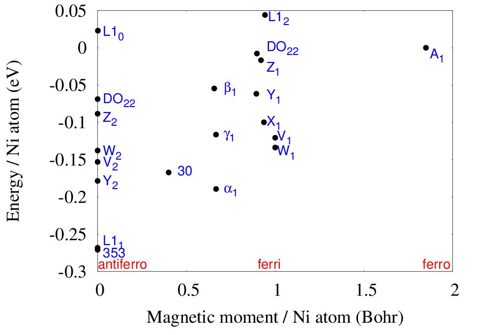
Figure 1: (Color Online)Energy and magnetic moment of PBE/LAPW calculated configurations. Configurations with zero magnetic moment are exactly antiferromagnetic. The configuration with moment $\simeq 2$ is ferromagnetic. In between one has many possible ferrimagnetic states. The energy zero is the ferromagnetic arrangement $A_{1}$.

II.1 2.a. Cluster expansions

For alloys one uses the well known cluster expansion (CE) Sanchez

$$E(\sigma)=\sum_{j,k}J_{j}\Pi_{j,k}(\sigma)=\sum_{j}J_{j}\bar{\Pi}_{j}(\sigma)$$ (1)

where $E$ is the energy (per $Ni$ atom) of a configuration $\sigma$ of atoms $A$ and $B$ or spins $up$ and $down$ in a lattice. $\Pi_{j,k}$ is a product of Ising spins $S=1\ or\ -1$ at the vertices of a polyhedron $j$ drawn in the lattice. $\Pi$ depends on the configuration. There are tables and codes for the calculation of $\Pi_{j,k}$ Ferreira ; Ceder . $k$ numbers identical polyhedron displaced by translation or rotation symmetry operations, and $\bar{\Pi}_{j}$ is the average of $\Pi_{j,k}$ in the set of identical polyhedra Laks . $J_{j}$ are the $Ni$-$Ni$ interaction parameters. In the case of $NiO$ we have 18 configurations in our data set, thus we can find at most 18 interaction parameters $J_{j}$, assuming all the other interactions are negligible.

The whole procedure to find the CE is the following. Assume we have first-principles calculated more configurations than the number of $J_{j}^{{}^{\prime}}$s we plan to use in our CE. Then we find the $J_{j}^{{}^{\prime}}$s by least square error fit . In many instances this procedure will lead to a very wrong CE, and we must have a recipe to choose the size of the CE and which interactions $J_{j}$ to use. The recipe was formulated in the reference Ceder and frequently leads to short CE’s Guima et al . Reference Ceder uses a figure of merit that corresponds to the predictive power of the set of interactions. The idea is the following. Let $\sigma$ be a configuration of the set, let $e(\sigma)$ be its first-principles total energy per $Ni$ atom, let $j$ be an interaction (figure) of the set, and $J_{j}$ its value, and let $E(\sigma)$ calculated according to Eq. 1 be the cluster expansion approximation to the true value $e(\sigma)$.

If the set of interactions and the set of configurations are given, the interaction values $J_{j}$ should be chosen so to minimize the rms error

$$rms^{2}=\frac{1}{N}\sum_{\sigma=1}^{N}[e(\sigma)-E(\sigma)]^{2}=min.$$ (2)

This minimization brings no information on the predictive power of the set of interactions. To know its predictive power we consider the set of configurations with one of them excluded, say configuration $\omega$. With this exclusion we recalculate the values $J_{j}$, again using Eq. 2, and obtain the approximation $\hat{E}(\omega)$ to the first-principle calculated value corresponding to the excluded configuration. Following reference Ceder we define the ‘cross-validation’ (CV) figure of merit as

$$CV^{2}=\frac{1}{N}\sum_{\omega=1}^{N}[e(\omega)-\hat{E}(\omega)]^{2}$$ (3)

in other words, we sum squared errors for each configuration when it is excluded from the set. As a practical way to calculate $CV$ one proves the relation

$$e(\sigma)-\hat{E}(\sigma)=[e(\sigma)-E(\sigma)]\left[1-\sum_{j,m}\Pi_{j}(\sigma)Q(j,m)^{-1}\Pi_{m}(\sigma)\right]^{-1}$$ (4)

where $Q$ is the matrix

$$Q(j,m)=Q(m,j)=\sum_{\sigma}\Pi_{m}(\sigma)\Pi_{j}(\sigma).$$

Eq. 4 shows that $CV$ is always greater than $rms$ error.

In the case of $NiO$ we started from the first 13 nearest neighbour pair interaction and the four-body nearest neighbour interaction (a regular tetrahedron of lattice sites). The cross-validation $CV$ was decreased when we reduced the number of interactions. We ended with one CE with the first two nearest-neighbour pair interactions, named $J_{2}$ and $K_{2}$, and the tetrahedron interaction $J_{4}$. The labels and definitions of these interactions follow references US-BR ; Laks ; gang ; gang2 . For this CE, the cross-validation was $CV=0.01384~{}eV$ and the root-mean square error was $rms=0.01244~{}eV$. It is amazing that longer-range pair interactions only damage the CE. For comparison, this CE predicted an energy of $-0.2705~{}eV$ for the data-set configuration $L1_{1}$ while the LAPW result is $-0.2662~{}eV$. The zero of energy being used is the ferromagnetic $A_{1}$ configuration in Fig. 1.

II.2 2.b. The ground state

Using the CE and scanning our file of configurations, which has all configurations up to 8 $Ni$ atoms per cell, we found a configuration with number $353$ which, together with configuration $L1_{1}$ is the ground state of rock-salt $NiO$. This same result was obtained with a CE without the four body interaction but with 3 pair interactions instead of 2. This latter CE had slightly larger $CV$. The CE predicts $E($353$)=-0.2873~{}eV$ and the all-electron LAPW code gives $E($353$)=-0.2708~{}eV$. The true ground state, $353$ or $L1_{1}$, depends on the parameters of the calculation, such as the size of the wave-function, charge density and potential expansions, exchange-correlation approximation and could not be determined. In all cases the CE results are consistent with first-principles. For instance, using the exchange of Ref. PBEsol the difference between the energies per $Ni$ for $L1_{1}$ and $353$ is only $0.0006~{}eV/Ni$. This degeneracy is not related to symmetry which is very different for the two configurations. $353$ has space group $227\ Fd-3m$, while $L1_{1}$ is rhombohedral ($166\ R-3m$). Each $Ni$ atom of configuration $353$ has 6 first-neighbours with the same spin and 6 with opposite spin, as in the configuration $L1_{1}$, though with a different space distribution. The other antiferromagnet of Fig. 1 do not have this 6/6 distribution of neighbours.

Configuration $L1_{1}$ is an alternation of spin-up and spin-down planes along the cubic direction $(111)$. Its energy may be lowered by a shear strain deformation along this direction. The gain in energy is in the order of a fraction of $meV$, thus unable to decide on the ground state. Configuration $353$ is highly symmetrical, with space group Fd-3m. In units of a simple cubic lattice parameter the atomic positions are:

• Spin up: (0.5,0,0); (0.25,0.25,0.5); (0.75,0.5,0.75); (0,0.75,0.25)

• Spin down: (0.25,0,0.25); (0.5,0.25,0.75); (0,0.5,0.5); (0.75,0.75,0)

One readily sees that, with respect to a vector (210), the spin up atoms occupy planes positioned at z=-0.25, 0., 0.75, 1., 1.75, 2., … and spin down are at z=0.25, 0.5, 1.25, 1.5, 2.25, … The 12 $Ni$ neighbours of each $Ni$ atom in configuration $353$ are in two octahedra, one made of spins up, the other with spins down.

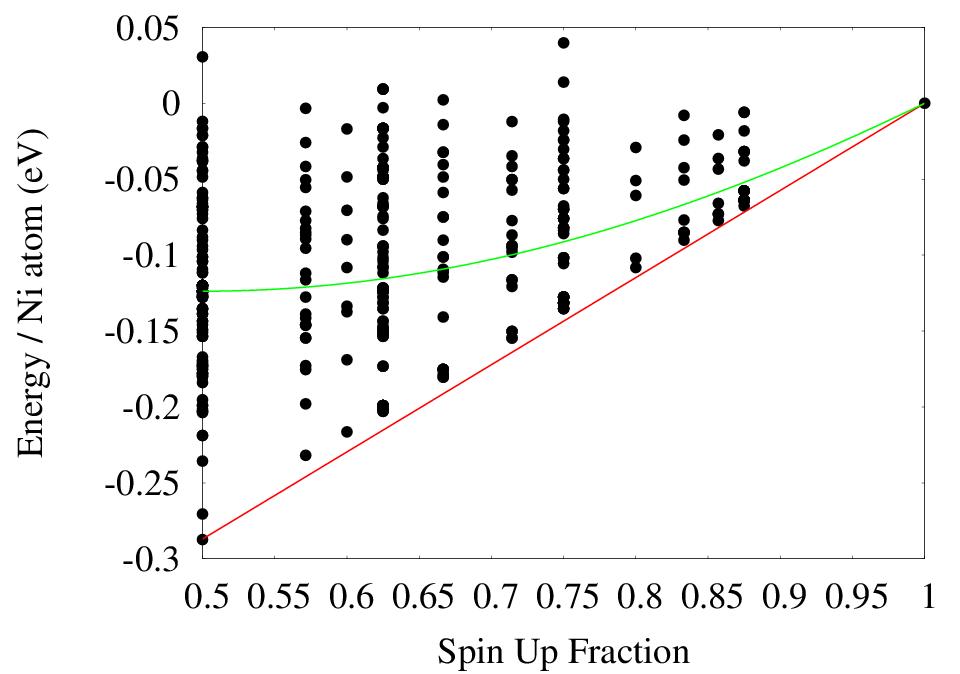
Figure 2: (Color Online)Energy for each of the 365 configurations in the file containing all with up to 8 $Ni$ atoms per cell against the fraction of spin up $Ni$ atoms. The straight line joining the antiferromagnetic ground state at $x=0.5$ to the ferromagnetic $x=1$ means the locus of the two-phase mixtures of anti- and ferromagnet. The curved line is the paramagnetic phase with spins randomly oriented. Clearly all ferrimagnetic solutions decay into the two-phase mixture showing the impossibility of ferrimagnetic $NiO$

Fig. 2 hints at the impossibility of $NiO$ presenting a ferrimagnetic phase. As explained in the Fig., such phase would decay into a two-phase mixture. The argument is based on our file containing 365 configurations. Ordered configurations with more than 8 Nickel atoms per cell would be difficult to prepare, either in Nature or in a Lab.

II.3 2.c. Monte Carlo results

Having the cluster expansion parameters, it is not difficult to run Monte Carlo calculations, following the Metropolis algorithm Metropolis . Fig. 3 shows the Energy (Enthalpy) function of temperature. At low temperatures, the ground state is $353$, not $L1_{1}$, for the present calculation, or a phase with the same $\bar{\Pi}$ for the nearest-neighbour pair, for the second-neighbour pair, and for the tetrahedron first-neighbour 4-body interaction. Ising model leads to a much too high transition temperature, even higher than the melting point. In the Fig. caption we present two reasons why the Ising model fails to determine the Thermodynamics.

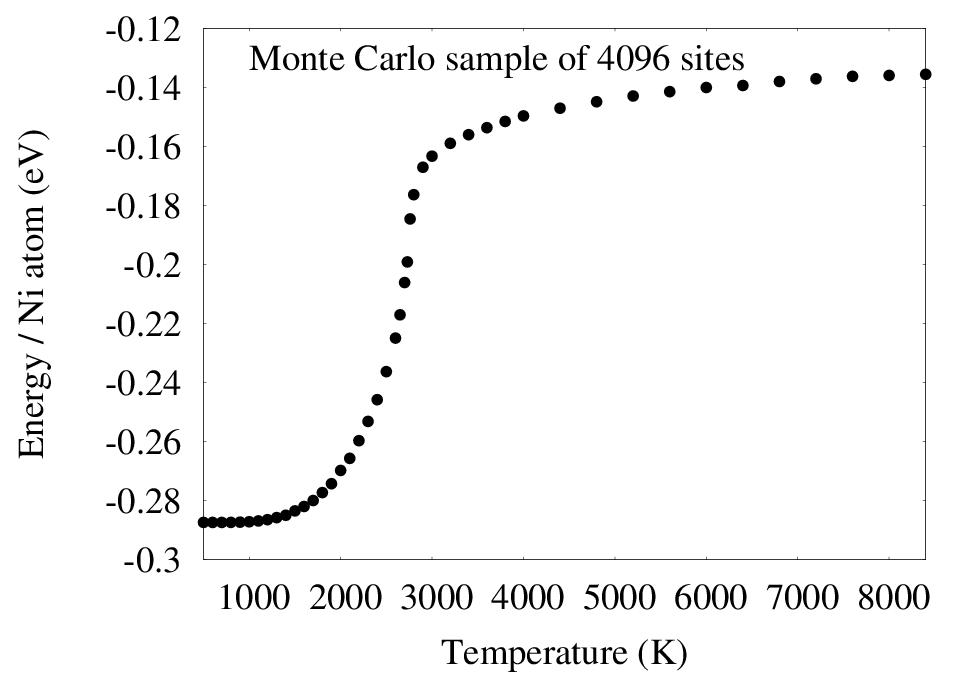
Figure 3: Energy as function of $T$ for the Monte Carlo runs. The phase transition happens at $T=2750\pm 10K$. The phase at low temperatures is certainly $353$, not $L1_{1}$, resulting from the present choice of first-principles calculation parameters. One distinguishes the two phases by the value of $\bar{\Pi}(\sigma)$ corresponding to the nearest-neighbour tetrahedron of sites. The calculated transition temperature is much too high, even higher than the melting temperature. Two reasons concur to that: 1 - We are using an Ising Hamiltonian, not Heisenberg For instance, 2D Ising models have ordered phases, Heisenberg models have not because the transverse spin components allow paths of relaxation. 2 - We are assuming that sublattice magnetizations are unique and do not depend on spin configuration of the lattice, that is, given the concentration $x$ the magnetization is known. Fig. 1 shows the real situation where the magnetization can fluctuate to some extent for configurations with the same $x$.

III 3. Electronic Excitations

The literature on the electronic excitations of $NiO$ is very rich. It was accepted as a Mott insulator and many theoretical methods were applied, to account for the strong correlations, and based on band calculations gap-theo ; Peter ; Das or based on cluster calculations Eder . Without reviewing the many works and techniques, we decided to give a chance to a very successful technique we developed for the calculation of semiconductors: LDA/GGA-1/2 Guima et al ; LDA-1/2 ; AIP . It is not unusual that LDA/GGA-1/2 gives better results than GW or HSE bando We expect from our calculation: 1 - to produce an insulating $NiO$; 2 - a band gap of about 4.0 eV; 3 - smaller band gaps in the order of 1.0 eV. Expectations 2 and 3 are incompatible, unless more than one valence band is playing in the excitations.

Pure Kohn and Sham (KS) methods are good for the calculation of total energies, as we used throughout the preceding section. When it comes to the calculation of excited states, the KS band structures present very important errors. In the case of semiconductors, one misses band gaps for the small gap semiconductors and, generally, the KS gaps are smaller than true gaps and effective masses are lighter. These facts are universally recognized, and that is the reason for the increased use of $U$ in LDA+U, GGA+U, etc. Despite of this fact one sees attempts of performing single shots band calculations, simultaneously giving the total energy and the excitation spectrum. A recent attempt is the work of Tran et al Tran that uses exact-exchange as a reference method of calculation. At this point it is well to remind that half ionization methods beats true-exchange (Hartree-Fock) by a very large margin AIP .

Applying LDA/GGA-1/2 to $NiO$ is not straightforward. First we decided that the configuration to be investigated was the $L1_{1}$. We also made LDA/GGA-1/2 band calculations on the $353$ configuration but the results were wholly similar to those of $L1_{1}$. Secondly we must decide which atom, $Ni$ or $O$ should be half-ionized, and we chose the anion $O$, as is done for most LDA-1/2 calculations so far. Thirdly, since there are two $O$ in the cell, the ”self-energy potential” was halved for each $O$, as it is the usual practice, and multiplyed by $1/8$ in the case of 353. In the case of $NiO$, Fig. 4 shows the density of states for the pure GGA and for the GGA-1/2. The pure GGA result coincides with that of ref. Blaha2 and does not account for the $4.0eV$ band gap gap-exper . On the other hand the GGA-1/2 maintains the $1.0eV$ gap and opens a gap in the valence band. The method has one free parameter chosen to maximize the band gap. The free parameter $CUT$ was chosen to maximize the band gap between the first valence band and the 1st conduction band, that is the long horizontal arrow in the Fig. 4. The opened gap between the 1st valence and the 2nd valence exists in the region of $1.6\leq CUT\leq 3.7~{}a.u.$. Opening a gap is very common for LDA/GGA-1/2. In fact, most small gap semiconductors only present the band gap in the LDA/GGA-1/2, because in the pure GGA or LDA they are metals. It is simple to understand the two gaps: a) the gap of $4.0eV$ is the minority spin excitation $Ni^{++}O^{--}\longrightarrow Ni^{+}O^{-}$; b) The gap of $\simeq 1.0eV$ is the minority spin excitation $t\longrightarrow e$.

Our results were the following. Band gap between 1st valence band and 1st conduction band: 4.02 eV, in agreement with experimental BIS data. Band gap between 2nd valence band and 1st conduction band: 1.18 eV, consistent with the $10Dq$ for $Ni^{++}$. Observe that the 1st conduction band is very narrow meaning that the excited states in this band are much localized in the spin-down $Ni$ atom.

In what sense $NiO$ is a Mott insulator Mott ? First, aside from being a semiconductor. it is a very poor conductor, as one sees from the very narrow conduction band. Probably the conduction is mostly by holes in the first valence band. Second, the first band gap is a $Ni\ 3d\rightarrow Ni\ 3d$ transition which is optically forbidden. These features come from the GGA-1/2 bands and do not require any assumption on the electron-pair interaction.

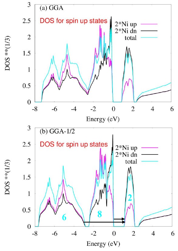
Figure 4: (Color Online)Total DOS and partial DOS projected on the $Ni$ atoms. The top panel (pure GGA(PBE)) equals the results of ref. Blaha2 . In the lower panel, the arrows indicate possible excitations. The numbers below the curves indicate the number of spin-up states in each pack. The first pack is mostly made of $O-p$ electrons. There are 6 such electrons with spin-up in this pack corresponding to the 2 $O$ atoms. The second pack is made of 5 $Ni-d$ electrons of the atom with spin-up plus 3 electrons of the atom with spin down. The third pack is already a conduction band and it is made of two states in the spin-down atom. As always, the cubic field splits the d-level into $3+2$ states, of which 3 states remain occupied and 2 states are empty forming the first conduction band. One notices that the first conduction band is very narrow, meaning that it conducts poorly.

The band gap between the highest valence and the first conduction bands corresponds to $10Dq\simeq 1.0eV$ of splitting $d$-states by a cubic field, compatible with the standard value for the $Ni^{++}$ ion in aqueous solution 10Dq . In studying these curves, one has to pay attention to the following facts: 1 - what is being plotted is the cubic root of the DOS, not the DOS itself; 2 - the partial DOS for the $Ni$ atoms is being doubled.

It must be mentioned that this application of LDA/GGA-1/2 to $NiO$ is not the first we made. In 2009 we presented results of another calculation old where both the $Ni$ and the $O$ atoms were half-ionized. In that case there was no gap separating the two parts of the valence band. We much prefer the present results because it is calculated with the most standard techniques within GGA-1/2. Further, the conduction band at $4.0eV$ (or $1.0eV$ counted from the top of the valence band) is d-like in the present version instead of s-like of the older version.

IV 4. Summary

In this work we made an unusual study of $NiO$, considered as an alloy of spin-up and spin-down $Ni$ atoms. We could not find a stable ferrimagnetic phase, which is satisfying because no such phase was ever detected. But we were able to calculate an antiferromagnetic phase $Ni_{8}O_{8}$ degenerate with the $L1_{1}$ phase, for all practical purposes.

In the second part of this work we restudied the one-electron excitations by means of the LDA/GGA-1/2 method. We used the most standard procedures within that method and found two band gaps, corresponding to a split of the valence band, and features of a Mott insulator. Hopefully, our results again match experiment.

References

- (1) D. de Fontaine, in Solid State Physics. edited by H. Ehrenreich, F. Seitz, and D. Turnbull (Academic, New York, 1979), Vol. 34, p. 73.
- (2) J. M. Sanchez, F. Ducastelle, and D. Gratias, Physica 128A 334 (1984).
- (3) P. Blaha, K. Schwarz, G. K. H. Madsen, D. Kvasnicka, J. Luitz, ”An Augmented PlaneWave + Local Orbitals Program for Calculating Crystal Properties”, Techn. Universität Wien, Getreidemarkt 9/156, A-1060Wien/Austria (2012).
- (4) . C. Toroker, D. K. Kanan, N. Alidoust, L. Y. Isseroff, P. Liaob and E. A. Carter, Phys. Chem. Chem. Phys., 13, 16644-16654 (2011); M. C. Toroker and E. C. Carter, J. Mater. Chem. A 1 2474-2484 (2013).
- (5) F. Tran and P. Blaha, Phys. Rev. Lett. 102, 226401 (2009).
- (6) Suvadip Das, John E. Coulter, and Efstratios Manousakis, Phys. Rev. B 91, 115105 (2015).
- (7) R. Eder, Phys. Rev. B 78, 115111 (2008).
- (8) G. A. Sawatzky and J. W. Allen, Phys. Rev. Lett. 53, 2339 (1984).
- (9) R. Merlin, Phys. Rev. Letters 54 2727 (1985).
- (10) B.Fromme, “D-d excitations in transition metal oxides: a spin-polarized electron energy-loss spectroscopy (SPEELS) study” (Springer-Verlag, Berlin-Heidelberg) 2001.
- (11) S. Huotari, T. Pylkkänen, G. Vankó, R. Verbeni, P. Glatzel, and G. Monaco, Phys. Rev. B, 78 041102(R) (2008) .
- (12) F. Müller and S. Hüfner, Phys. Rev. B, 78 085438 (2008).
- (13) Z. W. Lu, S.-H. Wei. A. Zunger, S. Frota-Pessoa, L. G. Ferreira, Phys. Rev. B 44 512 (1991-II).
- (14) D. B. Laks, L. G. Ferreira, S. Froyen, A. Zunger, Phys. Rev. N 46 12587 (1992-I).
- (15) V. Ozoliņš, C. Wolverton, and A. Zunger, Phys. Rev. B 57, 6427 (1998).
- (16) L. G. Ferreira, V. Ozoliņš, and A. Zunger, Phys. Rev. B 60 1687 (1999).
- (17) J. P. Perdew, S. Burke, and M. Ernzerhof, Phys. Rev. Let. 77 3865 (1996).
- (18) Because of a defective cluster expansion that pointed to its importance.
- (19) L.G. Ferreira, S.-H. Wei e A. Zunger, Int. J. of Supercomputer Applications 5, 34-56 (1991)
- (20) A. van de Walle and G. Ceder, J. Phase Equilib. 23, 348 (2002).
- (21) L. G. Ferreira, M. Marques, L. K. Teles, Phys. Rev. B 74, 075324 (2006).
- (22) J. P. Perdew, S. Kurth, J. Zupan, and P. Blaha, Phys. Rev. Let. 82, 2544 (1999).
- (23) N. Metropolis, A. W. Rosenbluth, M. N. Rosenbluth, A. H. Teller, and E. Teller, J. Chem. Phys. 21, 1087 (1953).
- (24) N. F. Mott, Proceedings of the Physical Society A 62, 416 (1949).
- (25) L. G. Ferreira. M. Marques, L. K. Teles, Phys. Rev B 78, 125116 (2008).
- (26) L. G. Ferreira. M. Marques, L. K. Teles, AIP ADVANCES 1, 032119 (2011).
- (27) O. P. Silva Filho, M. Ribeiro, Jr., R. R. Pelá, L. K. Teles, L. G. Ferreira, and M. Marques, J. App. Phys. 114 033709 (2013).
- (28) Walid Hetaba, Peter Blaha, Fabien Tran, and Peter Schattschneider1, Phys. Rev. B 85, 205108 (2012).
- (29) Fabien Tran, Peter Blaha, Markus Betzinger, Stefan Blügel, Phys. Rev. B 91, 165121 (2015).
- (30) Hydrated ion in solution. Ni2+ = 8600 cm-1. D. S. McClure, ”Solid State Phys. Advances in Research and Applications”, 9, 399 (1959). Quoted by A. Abragan and B. Bleaney, ”Electron Paramagnetic Resonance of Transition Ions”, OUP Oxford (2012), p. 378
- (31) L. G. Ferreira, L. K. Teles, and M. Marques, arXiv:0910.4485v1 [cond-mat.mtrl-sci] 23 Oct 2009.