A theory of 2+1D bosonic topological orders

Abstract

In primary school, we were told that there are four phases of matter: solid, liquid, gas, and plasma. In college, we learned that there are much more than four phases of matter, such as hundreds of crystal phases, liquid crystal phases, ferromagnet, anti-ferromagnet, superfluid, etc . Those phases of matter are so rich, it is amazing that they can be understood systematically by the symmetry breaking theory of Landau. However, there are even more interesting phases of matter that are beyond Landau symmetry breaking theory. In this paper, we review new “topological” phenomena, such as topological degeneracy, that reveal the existence of those new zero-temperature phases – topologically ordered phases. Microscopically, topologically orders are originated from the patterns of long-range entanglement in the ground states. As a truly new type of order and a truly new kind of phenomena, topological order and long-range entanglement require a new language and a new mathematical framework, such as unitary fusion category and modular tensor category to describe them. In this paper, we will describe a simple mathematical framework based on measurable quantities of topological orders $(S,T,c)$ proposed around 1989. The framework allows us to systematically describe all 2+1D bosonic topological orders (i.e. topological orders in local bosonic/spin/qubit systems).

I Introduction

I.1 Orders, phase transitions, and symmetries

Condensed matter physics is a branch of science that study various properties of all kinds of materials, such as mechanical properties, hydrodynamic properties, electric properties, magnetic properties, optical properties, thermal properties, etc . Since there are so many different kinds of materials with vastly varying properties, not surprisingly, condensed matter physics is a very rich field. Usually for each kind of material, we need a different theory (or model) to explain its properties. So there are many different theories and models to explain various properties of different materials.

However, after seeing many different type of theories/models for condensed matter systems, a common theme among those theories start to emerge. The common theme is the principle of emergence, which states that the properties of a material are mainly determined by how particles are organized in the material. Different organizations of particles lead to different materials and/or different phases of matter, which in turn leads to different properties of materials.

Typically, one may think that the properties of a material should be determined by the components that form the material. However, this simple intuition is incorrect, since all the materials are made of same three components: electrons, protons and neutrons. So we cannot use the richness of the components to understand the richness of the materials. The various properties of different materials originate from various ways in which the particles are organized. The organizations of the particles are called orders. The orders (the organizations of particles) determine the physics properties of a material.

Therefore, according to the principle of emergence, the key to understand a material is to understand how electrons, protons and neutrons are organized in the material. However, to develop a theory for all possible organizations of particles, we need to have a more precise description/definition of organizations of particles.

First, we need to find a way to determine if two organizations of particles should be regard as the same (or more precisely, belong to the same class or belong to the same phase) or not. Here, we need to rely on the phenomena of phase transition. If we can deform the system (such as changing temperature, magnetic field, or other parameters of the system) in such a way that the state of the system before the deformation and the state of the system after the deformation are smoothly connected without any phase transition, then we say the two states before and after the deformation belong to the same phase and the particles in the two states are regarded to have the same organization. If there is no way to deform the system to connect two states in a smooth way, then, the two states belong to two different phases and the particles in the two states are regarded to have to two different organizations.

We note that our definition of organizations is a definition of an equivalent class. Two states that can be connected without a phase transition are defined to be equivalent. The equivalent class defined in this way is called the universality class. Two states with different organizations can also be said to belong to different universality classes. We introduce a formal name “order” to refer to the “organization” defined above.

Based on a deep insight into phase and phase transition, Landau developed a general theory of orders as well as transitions between different phases of matterLandau (1937); Ginzburg and Landau (1950); Landau and Lifschitz (1958). Landau points out that the reason that different phases (or orders) are different is because they have different symmetries. A phase transition is simply a transition that changes the symmetry. Introducing order parameters that transform non-trivially under the symmetry transformations, Ginzburg and Landau developed Ginzburg-Landau theory, which became the standard theory for phase and phase transition.Ginzburg and Landau (1950) For example, in Ginzburg-Landau theory, the order parameter can be used to characterize different symmetry breaking phase: if the order parameter is zero, then we are in a symmetric phase; if the order parameter is non-zero, then we are in a symmetry break phase. The symmetry breaking phase transition is the process in which the order parameter change from zero to non-zero.

Landau’s theory is very successful. Using Landau’s theory and the related group theory for symmetries, we can classify all of the 230 different kinds of crystals that can exist in three dimensions. By determining how symmetry changes across a continuous phase transition, we can obtain the critical properties of the phase transition. The symmetry breaking also provides the origin of many gapless excitations, such as phonons, spin waves, etc., which determine the low-energy properties of many systems.Nambu (1960); Goldstone (1961) Many of the properties of those excitations, including their gaplessness, are directly determined by the symmetry.

As Landau’s symmetry-breaking theory has such a broad and fundamental impact on our understanding of matter, it became a corner-stone of condensed matter theory. The picture painted by Landau’s theory is so satisfactory that one starts to have a feeling that we understand, at least in principle, all kinds of orders that matter can have. One starts to have a feeling of seeing the beginning of the end of the condensed matter theory.

However, through the researches in last 25 years, a different picture starts to emerge. It appears that what we have seen is just the end of beginning. There is a whole new world ahead of us waiting to be explored. A peek into the new world is offered by the discovery of fractional quantum Hall (FQH) effect.Tsui et al. (1982) Another peek is offered by the discovery of high $T_{c}$ superconductors.Bednorz and Mueller (1986) Both phenomena are completely beyond the paradigm of Landau’s symmetry breaking theory. Rapid and exciting developments in FQH effect and in high $T_{c}$ superconductivity resulted in many new ideas and new concepts. Looking back at those new developments, it becomes more and more clear that, in last 25 years, we were actually witnessing an emergence of a new theme in condensed matter physics. The new theme is associated with new kinds of orders, new states of matter and new class of materials beyond Landau’s symmetry breaking theory. This is an exciting time for condensed matter physics. The new paradigm may even have an impact in our understanding of fundamental questions of nature – the emergence of elementary particles and the four fundamental interactions.Wen (2002, 2003); Levin and Wen (2006); Wen (2013a); You et al. (2014); You and Xu (2015)

I.2 The discovery of topological order

After the discovery of high $T_{c}$ superconductors in 1986,Bednorz and Mueller (1986) some theorists believed that quantum spin liquids play a key role in understanding high $T_{c}$ superconductorsAnderson (1987) and started to construct and study various spin liquids.Baskaran et al. (1987); Affleck and Marston (1988); Rokhsar and Kivelson (1988); Affleck et al. (1988); Dagotto et al. (1988) Despite the success of Landau symmetry-breaking theory in describing all kind of states, the theory cannot explain and does not even allow the existence of spin liquids. This leads many theorists to doubt the very existence of spin liquids. In 1987, a special kind of spin liquids – chiral spin stateKalmeyer and Laughlin (1987); Wen et al. (1989) – was introduced in an attempt to explain high temperature superconductivity. In contrast to many other proposed spin liquids at that time, the chiral spin liquid was shown to correspond to a stable zero-temperature phase and is more likely to exist. At first, not believing Landau symmetry-breaking theory fails to describe spin liquids, people still wanted to use the symmetry breaking theory to characterize the chiral spin state. They identified the chiral spin state as a state that breaks the time reversal and parity symmetries, but not the spin rotation and translation symmetries.Wen et al. (1989) However, it was quickly realized that there are many different chiral spin states (with different spinon statistics and spin Hall conductances) that have exactly the same symmetry, so symmetry alone is not enough to characterize different chiral spin states. This means that the chiral spin states contain a new kind of order that is beyond symmetry description.Wen (1989) This new kind of order was namedWen (1990a) topological order.

But experiments soon indicated that high-temperature superconductors do not break the time reversal and parity symmetries and chiral spin states do not describe high-temperature superconductors.Lawrence et al. (1992) Thus the concept of topological order became a concept with no experimental realization.

Although the concept of topological order is introduced in a theoretical study, about a state that is not known to exist in nature, this does not prevent topological order to become a useful concept. As we will see later that the concept of topological order contains inherent self consistency and stability. If we believe in nature’s richness, all nice concepts should be realized one way or another. The concept of topological order is not an exception.

Long before the discovery of high $T_{c}$ superconductors, Tsui, Stormer, and Gossard discovered FQH effect,Tsui et al. (1982) such as the filling fraction $\nu=1/m$ Laughlin stateLaughlin (1983)

$$\Psi_{\nu=1/m}(\{z_{i}\})=\prod(z_{i}-z_{j})^{m}\hskip 1.0pt\mathrm{e}^{-\frac{1}{4}\sum|z_{i}|^{2}}$$ (1)

where $z_{i}=x_{i}+\hskip 1.0pt\mathrm{i}\hskip 1.0pty_{i}$. People realized that the FQH states are new states of matter. However, influenced by the previous success of Landau’s symmetry breaking theory, people still want to use order parameters and long range correlations to describe the FQH states.Girvin and MacDonald (1987); Zhang et al. (1989); Read (1989) But, if we concentrate on physical measurable quantities, we will see that all those different FQH states have exactly the same symmetry and conclude that we cannot use Landau symmetry-breaking theory and symmetry breaking order parameters to describe different orders in FQH states. So the order parameters and long range correlations of local operators are not the correct way to describe the internal structures of FQH states. In fact, just like chiral spin states, FQH states also contain new kind of orders beyond Landau’s symmetry breaking theory. Different FQH states are also described by different topological orders.Wen and Niu (1990) Thus the concept of topological order does have experimental realizations in FQH systems.

In addition to the Laughlin states, more exotic non-abelian FQH states were proposed in 1991 by two independent works. LABEL:Wnab pointed out that the FQH states described by wave functions

$$\Psi_{\nu=n/m}(\{z_{i}\}) =[\chi_{n}(\{z_{i}\})]^{m},$$

$$\text{ or }\Psi_{\nu=n/(m+n)}(\{z_{i}\}) =\chi_{1}(\{z_{i}\})[\chi_{n}(\{z_{i}\})]^{m}$$ (2)

have excitations with non-abelian statistics, where $\chi_{n}$ is the fermion wave function of $n$-filled Landau levels. The edge of the above FQH states are described by $U(1)^{nm}/SU(m)_{n}$ or $U(1)^{nm+1}/SU(m)_{n}$ Kac-Moody current algebra.Wen (1990b, 1992, 1995); Blok and Wen (1992) Those results were obtained by deriving their low energy effective $SU(m)$ level $n$ Chern-Simons theory or $U(1)\times SU(m)$ level $n$ Chern-Simons theory. In the same year, LABEL:MR9162 conjectured that the FQH state described by $p$-wave paired wave functionGreiter et al. (1991, 1992)

$$\Psi_{\nu=1/2}={\cal A}\Big{[}\frac{1}{z_{1}-z_{2}}\frac{1}{z_{3}-z_{4}}\cdots\Big{]}\hskip 1.0pt\mathrm{e}^{-\frac{1}{4}\sum|z_{i}|^{2}}\prod(z_{i}-z_{j})^{2}.$$ (3)

has excitations with non-abelian statistics. Its edge states were studied numerically in LABEL:Wnabhalf and were found to be described by a $c=1$ chiral-boson conformal field theory (CFT) plus a $c=1/2$ Majorana fermion CFT. Such a result about the edge states supports the conjecture that the $p$-wave paired FQH state is non-abelian, since the edge for abelian FQH states always have integer chiral central charge $c$.Wen and Zee (1992); Wen (1992, 1995) A few years later, the non-abelian statistics in $p$-wave paired wave function was also confirmed by its low energy effective $SO(5)$ Chern-Simons theory.Wen (1999)

It is interesting to point out that long before the discovery of FQH states, Onnes discovered superconductor in 1911.Onnes (1911) The Ginzburg-Landau theory for symmetry breaking phases is largely developed to explain superconductivity. However, the superconducting order, that motivates the Ginzburg-Landau theory for symmetry breaking, itself is not a symmetry breaking order. Superconducting order (in real life with dynamical $U(1)$ gauge field) is an order that is beyond Landau symmetry breaking theory. Superconducting order (in real life) is an topological order (or more precisely a $Z_{2}$ topological order).Wen (1991b); Hansson et al. (2004) It is quite amazing that the experimental discovery of superconducting order did not lead to a theory of topological order, but instead, lead to a theory of symmetry breaking order, that fails to describe superconducting order itself.

II What is topological order?

II.1 Topological ground state degeneracy

The above description of topological order is highly incomplete and highly unsatisfactory. This is because the characterization of topological order is through specifying what it is not: topological order is a kind of orders that cannot be described by symmetry breaking. But what is the topological order?

To appreciate the difficulty of describing topological order, let me tell a story about a tribe. The tribe uses a language that contains only four words for counting: one, two, three, and many-many. It is very hard for a tribe member to describe a naturally occurring phenomenon – a large herd of deers. He can only describe the number of deers in the herd by what it is not – the number is not one, nor two, nor three.

Similarly, the possible organizations of many particles in naturally occurring states can be very rich, much richer than those described by symmetry breaking. To describe the new orders (such as the topological orders), we need to introduce new tools and new languages. The richness of nature is not bounded by the known theoretical formalism. The Landau’s symmetry breaking theory corresponds to “one”, “two”, “three” which describes a small class of orders. Many other orders also exist in nature, but we do not know how to describe them. Therefore, we introduced terms like “spin liquid”, “non-Fermi liquid”, “exotic order”, “preformed pair”, “dynamical stripe”, etc . Just like the term “many many” in the above story, those terms mainly describe what it is not than what it is.

The symmetry breaking theory is the only language that we know to describe phases and orders. But topological order, by definition, cannot be described by the symmetry breaking theory. If we abandon the only language that we know, how can we say any thing? Where do we start to understand the topological order? So the development of topological order theory is mainly trying to come up with a proper way to name/label topological orders. We hope the name/label to carry information that allows us to derive all the universal properties of the corresponding topological order from its name/label.

To make progress, let us point out that, in physics, to define and to introduce a concept is to design an experiment (a laboratory one or a numerical one). We need to identify measurable quantities such that the measurement of those quantities facilitate the definition of the concept. So in physics, once you design an experiment, you define a concept. And only after you design an experiment, do you define a concept.

So what experiments or what measurable quantities define the concept of topological order? It was noted that a $\nu=1/m$ Laughlin FQH state has $m$ fold degenerate ground states on torus and a non-degenerate ground state on sphere.Yoshioka et al. (1983); Haldane (1983); Su (1984); Tao and Wu (1984); Niu et al. (1985); Haldane and Rezayi (1985); Avron and Seiler (1985); Haldane (1985) However, the different degeneracies was regarded as finite size and/or group theoretical effects without thermodynamical implications.

In LABEL:Wtop,Wrig,WNtop, it was shown that the ground state degeneracy of a chiral spin state or a FQH state is stable against any local perturbations, including random perturbations that break all the symmetries.Wen (1990a); Wen and Niu (1990) Thus the topology-dependent ground state degeneracies are a robust or universal property with important thermodynamical implications: the topology-dependent and topologically robust degeneracies can be used to define a phase (or a universality class) of a thermodynamical system (i.e. a system with a large size). So the topology-dependent ground state degeneracies is just what we are looking for: the measurable quantities (in a numerical experiment) that can be used to (partially) define topological order in chiral spin states and FQH states.Wen (1989); Wen and Niu (1990) Such kind of universal properties are also call topological invariants, since they are robust against any local perturbations.

We would like to remark that the ground state degeneracy discussed above is only an approximate degeneracy for a finite system, i.e. there is a small energy splitting $\epsilon$ between different degenerate ground states. The energy gap to other excited states is given by $\Delta$ (see Fig. 1). It was shown in LABEL:Wrig and LABEL:WNtop that, for chiral spin states and FQH states, $\epsilon$ is exponentially small: $\epsilon\sim e^{-L/\xi}$ while $\Delta$ is finite in the limit where the system size approaches infinite: $L\to\infty$.

The topology-dependent ground state degeneracy is an amazing phenomenon. In both FQH and chiral spin states, the correlation of any local operators are short ranged. This seems to imply that FQH and chiral spin states are “short sighted” and they cannot know the topology of space which is a global and long-distance property. However, the fact that ground state degeneracy does depend on the topology of space implies that FQH and chiral spin states are not “short sighted” and they do find a way to know the global and long-distance structure of space. So, despite the short-ranged correlations of all the local operators, the FQH and chiral spin states must contain certain hidden long-range structure. The robustness of the ground state degeneracy suggests that the hidden long-range structure in FQH/chiral-spin states is also robust and universal. A term topological order was introduced to describe such a “robust hidden long range structure”.Wen (1990a)

More recently, such a “robust hidden long range structure” was identified to be the long-range entanglement defined by local unitary transformations.Chen et al. (2010); Zeng and Wen (2015); Swingle and McGreevy (2014) Thus topological order is nothing but the pattern of long range entanglement. Different patterns of long-range entanglement (or different topological orders) correspond to different quantum phases. Chiral spin liquids,Kalmeyer and Laughlin (1987); Wen et al. (1989) integral/fractional quantum Hall statesvon Klitzing et al. (1980); Tsui et al. (1982); Laughlin (1983), $Z_{2}$ spin liquids,Read and Sachdev (1991); Wen (1991c); Moessner and Sondhi (2001) non-Abelian FQH states,Moore and Read (1991); Wen (1991a); Willett et al. (1987); Radu et al. (2008) etc are examples of topologically ordered or long-range entangled phases.

Figure 1: The energy levels of a topologically ordered state with a finite size. The splitting $\epsilon$ of the nearly degenerate ground states approaches to zero in the large-system limit.

II.2 Topological order and phase transitions

In section I.1, we define a quantum phase as a region bounded by lines of singularity in the ground state energy (or some other local quantities). In section II, we define a topologically ordered phase as a region characterized by a certain ground state degeneracy. Are these two definition self consistent? As one topologically ordered phase changes into another topologically ordered phase, the ground state degeneracy may change from one value to another value. So why a change in the ground state degeneracy corresponds to a singularity in some averages of local quantities?

Figure 2: Two types of phase transitions between two gapped states. (a) Energy levels of a Hamiltonian $H_{a}(g)$ as functions of the coupling constant $g$. The topologically order state for $g<g_{c}$ changes into a trivial state for $g>g_{c}$ via a first order phase transition. (b) Energy levels of a Hamiltonian $H_{b}(g)$ as functions of the coupling constant $g$. The topologically order state for $g<g_{c}$ changes into a trivial state for $g>g_{c}$ via a continuous phase transition. In this case, the ground state of $H_{b}(g_{c})$ is a quantum critical state.

We note that the ground state degeneracy that characterize topological order is robust again any perturbations. So a small change in the Hamiltonian will not change the ground state degeneracy. However, a large change of Hamiltonian can cause a change in ground state degeneracy. The ground state degeneracy can change in two different ways as described by Fig. 2.

In Fig. 2a, the ground state degeneracy changes due to an level crossing. The ground state energy has a discontinuous first order derivative at the crossing point. The corresponding phase transition is a first order phase transition.

Figure 3: An impossible $g$ dependence of energy levels.

Since the ground state degeneracy is robust against any perturbations, this means that the degenerate ground state wave functions are locally indistinguishable. The ground states cannot be split without losing the locally indistinguishable property. The only way to lose locally indistinguishable property is to develop a long range correlation i.e. closing the energy gap of other excitations. So, the situation described by Fig. 3 cannot happen. The possible situation is described by Fig. 2b, where the energy gap of the excitations closes as $g\to g_{c}$ and reopens as $g$ passes $g_{c}$. The closing of the energy gap allow the ground state degeneracy to change. The closing of the energy gap at $g_{c}$ cause a singularity in the ground state energy (or some other local quantities). Such a phase transition is a continuous phase transition.

We see that the change of ground state degeneracy of topologically ordered state and singularity in ground state energy always happen at the same place. Thus the topological ground state degeneracy characterize a phase and a change of the topological ground state degeneracy marks a phase transition.

II.3 Topological invariants – Towards a complete characterization of topological orders

Soon after the introduction of topological order through topologically robust and topology-dependent ground state degeneracies, it was realized that the topology-dependent degeneracies are not enough to characterize all different topological orders [note that, as discussed in section I.1, orders are defined through phase transitions]. Certain different topological orders can have exactly the same set of ground state degeneracies for all compact spaces.

To obtain a complete topological invariant that can fully characterize topological orders, in LABEL:Wrig,KW9327, it was conjectured that the non-Abelian geometric phasesWilczek and Zee (1984) (both the $U(1)$ part and the non-Abelian part) of degenerate ground states generated by the automorphism of Riemann surfaces can completely characterize different topological orders.Wen (1990a)

We note that an automorphism of a Riemann surface change the Hamiltonian $H$ defined on the surface to another Hamiltonian $H^{\prime}$ which is defined on the same surface. If we smoothly deform the Hamiltonian $H$ to $H^{\prime}$, plus the automorphism transformation at the end, we will get a family of Hamiltonians that form a “closed loop”.Wen (1990a); Keski-Vakkuri and Wen (1993) We can use such a loop-like deformation path of Hamiltonians, with their degenerate ground states, to define a non-Abelian geometric phase.Wilczek and Zee (1984) Thus, for every automorphism of Riemann surfaces, we can produce a non-Abelian geometric phase which is a unitary matrix.

Such a unitary matrix is uniquely determined by the automorphism (up to a path dependent over all $U(1)$ phase). To understand such a result, let us assume that the unitary matrix is not uniquely determined by the automorphism, i.e. a small change of deformation path leads to a different unitary matrix beyond the different over all $U(1)$ phase. This will mean that the small change of deformation path causes different phase shifts for different degenerate ground states. Since the small change of deformation path are local perturbations, the different phase shifts for different degenerate ground states will implies that the degenerate ground states are locally distinguishable, which contradict the robustness of the degeneracy against any local perturbations and the locally indistinguishable property of the degenerate ground states.

As a result, the above unitary matrices form a projective representation of automorphism group of Riemann surfaces.Wen (1990a); Kong and Wen (2014); Moradi and Wen (2014) The automorphism group $G_{\text{Aut}}$ contain a connected subgroup $G^{0}_{\text{Aut}}$. $G_{\text{Aut}}/G^{0}_{\text{Aut}}$ is the mapping class group (MCG). We note that the non-Abelian geometric phases for the automorphisms in $G^{0}_{\text{Aut}}$ are all pure $U(1)$ phases, since the loops that correspond to the automorphisms in $G^{0}_{\text{Aut}}$ are all contractible to a trivial point. Thus the non-Abelian geometric phase also generate a projective representation of MCG.

We see that the non-Abelian geometric phases contain a universal non-Abelian partWen (1990a); Keski-Vakkuri and Wen (1993) and a path dependent Abelian partWen (1990a, 2012). The non-Abelian part carries information about the projective representation of MCG. For torus, the MCG is $SL(2,\mathbb{Z})$, which is generate by a 90^∘ rotation and a Dehn twist. For such two generators of MCG, the associated non-Abelian geometric phases is denoted by $S$ and $T$, which are unitary matrices. $S$ and $T$ generate a projective representation of MCG $SL(2,\mathbb{Z})$ for torus.

The Abelian part of the non-Abelian geometric phases is also important: it is related to the gravitational Chern-Simons termKane and Fisher (1997); Hughes et al. (2012); Kong and Wen (2014); Bradlyn and Read (2015) and carries information about the chiral central charge $c$ for the gapless edge excitations.Wen (1992, 1995) The chiral central charge $c$ can be measured directly via the thermal Hall conductivity $K_{H}=c\frac{\pi}{6}\frac{k_{B}^{2}}{\hbar}T$ of the sample.Kane and Fisher (1997); Hughes et al. (2012)

It is believed that $(S,T,c)$ form a complete and one-to-one description of 2+1D topological orders, which is consistent with the previous conjecture in LABEL:Wrig. So $(S,T,c)$ are the new words, like “four”, “five”, “six”, “ten”, “eleven”, “twelve”, etc in our tribe story, that we are looking for, to describe/label topological orders. Since $(S,T,c)$ may completely describe 2+1D topological orders, we may be able develop a theory of 2+1D topological order based $(S,T,c)$.

II.4 Wave-function-overlap approach to obtain $S,T$

We like to mention that in addition to use non-Abelian geometric phases to obtain $(S,T)$ matrices, there are several other ways to obtain them.Zhang et al. (2012); Cincio and Vidal (2013); Zaletel et al. (2012); Tu et al. (2013) In particular, one can use wave function overlap to extract $(S,T)$ matrices directly from the degenerate ground states wave functions on torus, provided that the system have translation symmetry.Hung and Wen (2014); Moradi and Wen (2014); He et al. (2014); Mei and Wen (2015) (The non-Abelian-geometric-phase approach can obtain $(S,T)$ matrices even from systems without translation symmetry.) It was argued that for a system on a $d$-dimensional torus $T^{d}$ of volume $V$ with the set of topologically degenerate ground states $\{|\psi_{i}\rangle\}_{i=1}^{N}$, the overlaps of the degenerate ground states have the following form

$$\langle\psi_{i}|\hat{W}|\psi_{j}\rangle=e^{-fV+o(1/V)}M^{W}_{ij},$$ (4)

where $\hat{W}$ are transformations of the wave functions induced by the MCG transformations of the space $T^{d}\to T^{d}$, $f$ is a non-universal constant, and $M^{W}$ is an universal unitary matrix.

We know that a MCG transformation $\hat{W}$ maps the space $T^{d}$ to itself: $T^{d}\to T^{d}$. It transforms a ground state wave function $|\psi_{j}\rangle$ on space $T^{d}$ to another wave function $\hat{W}|\psi_{j}\rangle$ on the same space $T^{d}$. Since the MCG transformation $\hat{W}$ is not a symmetry of the Hamiltonian, the new wave function $\hat{W}|\psi_{j}\rangle$ is not longer a ground state of the Hamiltonian. So the overlap of $\hat{W}|\psi_{j}\rangle$ with a ground state $|\psi_{i}\rangle$ is exponentially small in large volume limit. $\langle\psi_{i}|\hat{W}|\psi_{j}\rangle\sim e^{-fV}$. It seems that such an overlap contains no useful universal information about topological order. What was discovered in LABEL:MW1418 is that if we separate out the volume dependent exponential factor, the volume-independent constant factor $M^{W}$ contains useful universal information about topological order.

We note that the volume-independent constant factor $M^{W}$ is a unitary matrix. In contrast to non-Abelian geometric phases, such a unitary matrix has no $U(1)$ phase ambiguity. Those unitary matrices (from different MCG transformations $\hat{W}$) form a representation of the MCG of the space $T^{d}$, $\texttt{MCG}(T^{d})=SL(d,\mathbb{Z})$, which is robust against any perturbations. For 2+1D cases, the MCG of the torus $T^{2}$ is generate by 90^∘ rotation $\hat{S}$ and Dehn twist $\hat{T}$. The corresponding unitary matrices $\hat{S}\to M^{S}\equiv S$ and $\hat{T}\to M^{T}\equiv T$ generate a unitary representation of $SL(2,\mathbb{Z})$ (instead of a projective representation as for the case of non-Abelian geometric phases). As a result, we can use a unitary representation of MCG, $(S,T)$, plus the chiral central charge $c$ to characterize all the 2+1D topological orders.

We also like to point out that we can always choose a so called excitation basis for the degenerate ground state (see Section D). In such a basis, $T$ is diagonal and $S_{1i}$ are real and positive. It is $(S,T)$ in such a basis, plus the chiral central charge $c$, that may fully characterize all the 2+1D topological orders.

II.5 The current systematic theories of topological orders

We like to remark that topological order (i.e. long-range entanglement) is truly a new phenomena. They require new mathematical language to describe them. Some early researches suggest that tensor category theoryFreedman et al. (2004); Levin and Wen (2005); Chen et al. (2010); Gu et al. (2015); Kitaev and Kong (2012); Gu et al. (2014) and simple current algebraMoore and Read (1991); Blok and Wen (1992); Wen and Wu (1994); Lu et al. (2010) (or pattern of zeros Wen and Wang (2008a, b); Barkeshli and Wen (2009); Seidel and Lee (2006); Bergholtz et al. (2006); Seidel and Yang (2008); Bernevig and Haldane (2008a, b, c)) may be part of the new mathematical language. Using tensor category theory, we have developed a systematic and quantitative theory that classify topological orders with gappable edge for 2+1D interacting boson and fermion systems.Levin and Wen (2005); Chen et al. (2010); Gu et al. (2015, 2014)

For 2+1D topological orders (with gapped or gapless edge) that have only Abelian statistics, we have a more complete and simpler result: we find that we can use integer $K$-matrices to classify all of them.Wen and Zee (1992) So the integer matrices $K$ are also the new words, like “4”, “5”, “6”, etc in our tribe story, that can be used to describe/label a subset of topological orders – Abelian topological orders. Such a $K$-label completely determine the low energy universal properties of the corresponding topological order. For example, the low energy effective theory for the topological order labeled by $K$ is given by the following $U(1)$ Chern-Simons theoryBlok and Wen (1990); Read (1990); Fröhlich and Kerler (1991); Wen and Zee (1992); Belov and Moore (2005); Kapustin and Saulina (2011); Wen (1995)

$${\cal L}=\frac{K_{IJ}}{4\pi}a_{I\mu}\partial_{\nu}a_{J\lambda}\epsilon^{\mu\nu\lambda}.$$ (5)

Such an effective theory or the topological order labeled by $K$ can be realized by a concrete physical system – a multi-layer FQH state:

$$\prod_{I;i<j}(z_{i}^{I}-z_{j}^{I})^{K_{II}}\prod_{I<J;i,j}(z_{i}^{I}-z_{j}^{J})^{K_{IJ}}\hskip 1.0pt\mathrm{e}^{-\frac{1}{4}\sum_{i,I}|z_{i}^{I}|^{2}},$$ (6)

where $z_{i}^{I}=x_{i}^{I}+\hskip 1.0pt\mathrm{i}\hskip 1.0pty_{i}^{I}$ is the coordinate of the $i^{\text{th}}$ particle in $I^{\text{th}}$ layer.

Certainly, the topological order described by $K$ are also described by $(S,T,c)$. The non-Abelian geometric phases for some canonical choices of path are calculated for the bosonic $K$ topological order described by eqn. (6):Wen (2012)

$$\tilde{T}_{\bm{\alpha}\bm{\beta}} =\hskip 1.0pt\mathrm{e}^{\frac{\hskip 1.0pt\mathrm{i}\hskip 1.0pt\pi}{12}(\bm{N}^{T}K\bm{N}-\bm{K}_{d}^{T}\bm{N})}\hskip 1.0pt\mathrm{e}^{\hskip 1.0pt\mathrm{i}\hskip 1.0pt\pi(\bm{\alpha}^{T}K\bm{\alpha}-\frac{c}{12})}\delta_{\bm{\alpha}\bm{\beta}}$$

$$\tilde{S}_{\bm{\alpha}\bm{\beta}} =(-)^{(\bm{N}^{T}K\bm{N}-\bm{K}_{d}^{T}\bm{N})/2}\frac{\hskip 1.0pt\mathrm{e}^{-\hskip 1.0pt\mathrm{i}\hskip 1.0pt2\pi\bm{\beta}^{T}K\bm{\alpha}}}{\sqrt{|\det(K)|}},$$ (7)

where $c$ is the difference in the numbers of positive and negative eigenvalues of $K$, $\bm{K}_{d}^{T}=(K^{11},K^{22},\cdots,K^{\kappa\kappa})$ is two times the spin vector of the Abelian FQH state, and $\bm{N}^{T}=(N_{1},N_{2},\cdots,N_{\kappa})$ are the numbers of the bosonic “electrons” in each layer.Wen (1995) We see that the $U(1)$ factors depend on the number of electrons and are not universal. But we can isolate the universal non-Abelian part by taking the limit $\bm{N}\to 0$, and find

$$T_{\bm{\alpha}\bm{\beta}} =\hskip 1.0pt\mathrm{e}^{-\hskip 1.0pt\mathrm{i}\hskip 1.0pt2\pi\frac{c}{24}}\hskip 1.0pt\mathrm{e}^{\hskip 1.0pt\mathrm{i}\hskip 1.0pt\pi\bm{\alpha}^{T}K\bm{\alpha}}\delta_{\bm{\alpha}\bm{\beta}}$$

$$S_{\bm{\alpha}\bm{\beta}} =\frac{\hskip 1.0pt\mathrm{e}^{-\hskip 1.0pt\mathrm{i}\hskip 1.0pt2\pi\bm{\beta}^{T}K\bm{\alpha}}}{\sqrt{|\det(K)|}}=S_{\bm{\alpha}\bm{\beta}}.$$ (8)

We see that the universal non-Abelian part of the non-Abelian geometric phases determines $S$, $T$, and $c$ mod 24.

III Topological excitations

We have seen that we can use unitary representation of MCG and the chiral central charge, $(S,T,c)$, to characterize/label/name all the 2+1D topological orders. It is possible that $(S,T,c)$ is a full characterization of 2+1D topological orders, in the sense that all other universal properties of topological orders can be determined from the data $(S,T,c)$. In this section, we will discuss some other universal properties of 2+1D topological orders, and see how those universal properties are determined by the data $(S,T,c)$.

III.1 Local excitations and topological excitations

Topologically ordered states in 2+1D are characterized by their unusual particle-like excitations which may carry fractional/non-Abelian statistics. To understand and to classify particle-like excitations in topologically ordered states, it is important to understand the notions of local quasiparticle excitations and topological quasiparticle excitations.

First we define the notion of “particle-like” excitations. Consider a gapped system with translation symmetry. The ground state has a uniform energy density. If we have a state with an excitation, we can measure the energy distribution of the state over the space. If for some local area, the energy density is higher than ground state, while for the rest area the energy density is the same as ground state, one may say there is a “particle-like” excitation, or a quasiparticle, in this area (see Figure 4).

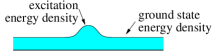
Figure 4: The energy density distribution of a quasiparticle.

Quasiparticles defined like this can be divided into two types. The first type can be created or annihilated by local operators, such as a spin flip. So, the first type of particle-like excitation is called local quasiparticle excitations. The second type cannot be created or annihilated by any finite number of local operators (in the infinite system size limit). In other words, the higher local energy density cannot be created or removed by any local operators in that area. The second type of particle-like excitation is called topological quasiparticle excitations.

From the notions of local quasiparticles and topological quasiparticles, we can further introduce the notion topological quasiparticle type, or simply, quasiparticle type. We say that local quasiparticles are of the trivial type, while topological quasiparticles are of nontrivial types. Two topological quasiparticles are of the same type if and only if they differ by local quasiparticles. In other words, we can turn one topological quasiparticle into the other one of the same type by applying some local operators.

III.2 Fusion space and internal degrees of freedom for the quasiparticles

The quasiparticles have locational degrees of freedom, as well as internal degrees of freedom.

To understand the notion of internal degrees of freedom, let us discuss another way to define quasiparticles:
Consider a gapped local Hamiltonian qubit system defined by a local Hamiltonian $H_{0}$ in $d$ dimensional space $M^{d}$ without boundary. A collection of quasiparticle excitations labeled by $i$ and located at $\bm{x}_{i}$ can be produced as gapped ground states of $H_{0}+\delta H$ where $\delta H$ is non-zero only near $\bm{x}_{i}$’s. By choosing different $\delta H$ we can create (or trap) all kinds of quasiparticles. We will use $i_{i}$ to label the type of the quasiparticle at $\bm{x}_{i}$. The gapped ground states of $H_{0}+\delta H$ may have a degeneracy $D(M^{d};i_{1},i_{2},\cdots)$ which depends on the quasiparticle types $i_{i}$ and the topology of the space $M^{d}$. The degeneracy is not exact, but becomes exact in the large space and large particle separation limit. We will use ${\cal V}(M^{d};i_{1},i_{2},\cdots)$ to denote the space of the degenerate ground states. If the Hamiltonian $H_{0}+\delta H$ is not gapped, we will say $D(M^{d};i_{1},i_{2},\cdots)=0$ (i.e., $\mathcal{V}(M^{d};i_{1},i_{2},\cdots)$ has zero dimension). If $H_{0}+\delta H$ is gapped, but if $\delta H$ also creates quasiparticles away from $\bm{x}_{i}$’s (indicated by the bump in the energy density away from $\bm{x}_{i}$’s), we will also say $D(M^{d};i_{1},i_{2},\cdots)=0$. (In this case quasiparticles at $\bm{x}_{i}$’s do not fuse to trivial quasiparticles.) So, if $D(M^{d};i_{1},i_{2},\cdots)>0$, $\delta H$ only creates/traps quasiparticles at $\bm{x}_{i}$’s.

If we choose the space to be a $d$-dimensional sphere $M^{d}=S^{d}$, then the number of the degenerate ground states, $D(S^{d};i_{1},i_{2},\cdots)$ represents the total number of internal degrees of freedom for the quasiparticles $i_{1},i_{2},\cdots)$. To obtain the number of internal degrees of freedom for type-$i$ quasiparticle, we consider the dimension $D(S^{d};i,i,\cdots,i)$ of the fusion space on $n$ type-$i$ particles on $S^{d}$. In large $n$ limit $D(S^{d};i,i,\cdots,i)$ has a form

$$\ln D(S^{d};i,i,\cdots,i)=n(\ln d_{i}+o(1/n)).$$ (9)

Here $d_{i}$ is called the quantum dimension of the type-$i$ particle, which describe the internal degrees of freedom the particle. For example, a spin-0 particle has a quantum dimension $d=1$, while a spin-1 particle has a quantum dimension $d=3$. For particles with abelian statistics, their quantum dimensions are always equal to $1$. For particles with non-abelian statistics, the quantum dimensions $d>1$, but in general the quantum dimensions $d$ may not be integers.

III.3 Simple type and composite type

Even after quotient out the local quasiparticle excitations, topological quasiparticle type still have two kinds: simple type and composite type.

We can also use the traping Hamiltonian $H_{0}+\delta H$ and the associated fusion space ${\cal V}(M^{d};i_{1},i_{2},\cdots)$ to understand the notion of simple type and composite type.

If the degeneracy $D(M^{d};i_{1},i_{2},\cdots)$ (the dimension of ${\cal V}(M^{d};i_{1},i_{2},\cdots)$) cannot not be lifted by any small local perturbation near $\bm{x}_{1}$, then the particle type $i_{1}$ at $\bm{x}_{1}$ is said to be simple. Otherwise, the particle type $i_{1}$ at $\bm{x}_{1}$ is said to be composite.

When $i_{1}$ is composite, the space of the degenerate ground states ${\cal V}(M^{d};i_{1},i_{2},i_{3},\cdots)$ has a direct sum decomposition:

$$\quad\ {\cal V}(M^{d};i_{1},i_{2},i_{3},\cdots)$$

$$={\cal V}(M^{d};j_{1},i_{2},i_{3},\cdots)\oplus{\cal V}(M^{d};k_{1},i_{2},i_{3},\cdots)$$

$$\ \ \ \ \ \ \ \oplus{\cal V}(M^{d};l_{1},i_{2},i_{3},\cdots)\oplus\cdots$$ (10)

where $j_{1}$, $k_{1}$, $l_{1}$, etc. are simple types. To see the above result, we note that when $i_{1}$ is composite the ground state degeneracy can be split by adding some small perturbations near $\bm{x}_{1}$. After splitting, the original degenerate ground states become groups of degenerate states, each group of degenerate states span the space $\mathcal{V}(M^{d};j_{1},i_{2},i_{3},\cdots)$ or $\mathcal{V}(M^{d};k_{1},i_{2},i_{3},\cdots)$ etc. which correspond to simple quasiparticle types at $\bm{x}_{1}$. The above decomposition allows us to denote the composite type $i_{1}$ as

$$i_{1}=j_{1}\oplus k_{1}\oplus l_{1}\oplus\cdots.$$ (11)

The degeneracy $D(M^{d};i_{1},i_{2},\cdots)$ for simple particle types $i_{i}$ is a universal property (i.e., a topological invariant) of the topologically ordered state. In this paper, when we said particle/topological type, we usually mean simple type. The number of simple types (including the trivial type) is also a topological invariant of the topological order. Such a number is referred as the rank of the topological order.

We have claimed that $(S,T,c)$ can determine all other topological invariants of a topological order, including its rank. Indeed, the dimension of the $S$ or $T$ matrices is the rank of the topological order.

III.4 Fusion of quasiparticles

When we fuse two simple types of topological particles $i$ and $j$ together, it may become a topological particle of a composite type:

$$i\otimes j=l=k_{1}\oplus k_{2}\oplus\cdots,$$ (12)

where $i,j,k_{i}$ are simple types and $l$ is a composite type. Here, we will use an integer tensor $N^{ij}_{k}$ to describe the quasiparticle fusion, where $i,j,k$ label simple types. Such an integer tensor $N^{ij}_{k}$ is referred as the fusion coefficients of the topological order, which is a universal property of the topologically ordered state.

When $N^{ij}_{k}=0$, the fusion of $i$ and $j$ does not contain $k$. When $N^{ij}_{k}=1$, the fusion of $i$ and $j$ contain one $k$: $i\otimes b=k\oplus k_{1}\oplus k_{2}\oplus\cdots$. When $N^{ij}_{k}=2$, the fusion of $i$ and $j$ contain two $k$’s: $i\otimes j=k\oplus k\oplus k_{1}\oplus k_{2}\oplus\cdots$. This way, we can denote that fusion of simple types as

$$i\otimes j=\oplus_{k}N^{ij}_{k}k.$$ (13)

In physics, the quasiparticle types always refer to simple types. The fusion rules $N^{ij}_{k}$ is a universal property of the topologically ordered state. The degeneracy $D(M^{d};i_{1},i_{2},\cdots)$ is determined completely by the fusion rules $N^{ij}_{k}$.

Let us then consider the fusion of 3 simple quasiparticles $i,j,k$. We may first fuse $i,j$, and then with $k$, $(i\otimes j)\otimes k=(\oplus_{m}N^{ij}_{m}m)\otimes k=\oplus_{l}(\sum_{m}N^{ij}_{m}N^{mk}_{l})l$. We may also first fuse $j,k$ and then with $i$, $i\otimes(j\otimes k)=i\otimes(\oplus_{m}N^{jk}_{m}m)=\oplus_{l}(\sum_{m}N^{im}_{l}N^{jk}_{m})l$. The two ways of fusion should produce the same result and this requires that

$$\sum_{m}N^{ij}_{m}N^{mk}_{l}=\sum_{m}N^{im}_{l}N^{jk}_{m}.$$ (14)

Note that here, we do not require $N^{ij}_{k}=N^{ji}_{k}$.

The fusion coefficients $N^{ij}_{k}$ are also topological invariants of the topological order. $(S,T,c)$ can determine such topological invariants. In fact, $S$ alone can determine $N^{ij}_{k}$:

$$N^{ij}_{k}=\sum_{l=1}^{n}\frac{S_{li}S_{lj}(S_{lk})^{*}}{S_{l1}}$$ (15)

which is the famous Verlinde formula.Verlinde (1988)

The internal degrees of freedom (i.e. the quantum dimension $d_{i}$) for the type-$i$ simple particle can be calculated directly from $N^{ij}_{k}$. In fact $d_{i}$ is the largest eigenvalue of the matrix $N_{i}$, whose elements are $(N_{i})_{kj}=N^{ij}_{k}$. We see that $S$ matrix determines the internal degrees of freedom of the simple particles.

III.5 Quasiparticle intrinsic spin

For 2+1D topological orders, the quasiparticles can also braid. We also need data to describe the braiding of the quasiparticles in addition to the fusion rules We will discuss the braiding in this and next subsections.

If we twist the quasiparticle at $\bm{x}_{1}$ by rotating $\delta H$ at $\bm{x}_{1}$ by 360^∘ (note that $\delta H$ at $\bm{x}_{1}$ has no rotational symmetry), all the degenerate ground states in $\mathcal{V}(M^{d};i_{1},i_{2},i_{3},\cdots)$ will acquire the same geometric phase $\hskip 1.0pt\mathrm{e}^{\hskip 1.0pt\mathrm{i}\hskip 1.0pt\theta_{i_{1}}}$ provided that the quasiparticle type $i_{1}$ is a simple type. This is because when $i_{1}$ is a simple type, no local perturbations near $\bm{x}_{1}$ can split the degeneracy. Thus the degenerate ground states are locally indistinguishable near $\bm{x}_{1}$. As a result, the 360^∘ rotation cause the same phase shift $\hskip 1.0pt\mathrm{e}^{\hskip 1.0pt\mathrm{i}\hskip 1.0pt\theta_{i_{1}}}$ for all the degenerate ground states. We will call $s_{i}=\frac{\theta_{i}}{2\pi}$ mod 1 the intrinsic spin (or simply spin) of the simple type $i$, which is another universal property of the topologically ordered state. $(S,T,c)$ can determine the topological invariants $s_{i}$ as well. In fact, $s_{i}$ mod 1 are given by the eigenvalues or the diagonal elements of $T$ and $c$:

$$\hskip 1.0pt\mathrm{e}^{\hskip 1.0pt\mathrm{i}\hskip 1.0pt2\pi s_{i}}=\hskip 1.0pt\mathrm{e}^{\hskip 1.0pt\mathrm{i}\hskip 1.0pt2\pi\frac{c}{24}}T_{ii}$$ (16)

(note that $T$ is diagonal in the excitation basis).

III.6 Quasiparticle mutual statistics

If we move the quasiparticle $i_{2}$ at $\bm{x}_{2}$ around the quasiparticle $i_{1}$ at $\bm{x}_{1}$, we will generate a non-Abelian geometric phase – a unitary transformation acting on the degenerate ground states in $\mathcal{V}(M^{d};i_{1},i_{2},i_{3},\cdots)$. Such a unitary transformation not only depends on the types $i_{1}$ and $i_{2}$, but also depends on the quasiparticles at other places. So, here we will consider three quasiparticles of simple types $i$, $j$, $\bar{k}$ on a 2D sphere $S^{2}$. The ground state degenerate space is ${\cal V}(S^{2};i,j,\bar{k})$. For some choices of $i$, $j$, $\bar{k}$, $D(S^{2};i,j,\bar{k})\geq 1$, which is the dimension of ${\cal V}(S^{2};i,j,\bar{k})$. Now, we move the quasiparticle $j$ around the quasiparticle $i$. All the degenerate ground states in ${\cal V}(S^{2};i,j,\bar{k})$ will acquire the same geometric phase

$$\hskip 1.0pt\mathrm{e}^{\hskip 1.0pt\mathrm{i}\hskip 1.0pt\theta_{ij}^{(k)}}=\dfrac{\hskip 1.0pt\mathrm{e}^{\hskip 1.0pt\mathrm{i}\hskip 1.0pt2\pi s_{k}}}{\hskip 1.0pt\mathrm{e}^{\hskip 1.0pt\mathrm{i}\hskip 1.0pt2\pi s_{i}}\hskip 1.0pt\mathrm{e}^{\hskip 1.0pt\mathrm{i}\hskip 1.0pt2\pi s_{j}}}.$$ (17)

This is because, in $\mathcal{V}(S^{2};i,j,\bar{k})$, the quasiparticles $i$ and $j$ fuse into $k$ (the anti-quasiparticle of $\bar{k}$). Moving quasiparticle $j$ around the quasiparticle $i$ plus rotating $i$ and $j$ respectively by 360^∘ is like rotating $k$ by 360^∘, i.e. $\hskip 1.0pt\mathrm{e}^{\hskip 1.0pt\mathrm{i}\hskip 1.0pt\theta_{ij}^{(k)}}\hskip 1.0pt\mathrm{e}^{\hskip 1.0pt\mathrm{i}\hskip 1.0pt2\pi s_{i}}\hskip 1.0pt\mathrm{e}^{\hskip 1.0pt\mathrm{i}\hskip 1.0pt2\pi s_{j}}=\hskip 1.0pt\mathrm{e}^{\hskip 1.0pt\mathrm{i}\hskip 1.0pt2\pi s_{k}}$. This leads to eqn. (17). We see that the quasiparticle mutual statistics is determined by the quasiparticle spin $s_{i}$ and the quasiparticle fusion rules $N^{ij}_{k}$. For this reason, we call the set of data $(N^{ij}_{k},s_{i})$ quasiparticle statistics.

In fact, in order for data $(N^{ij}_{k},s_{i})$ to describe a valid quasiparticle statistics, they must satisfy certain conditionsAndersen and Moore (1988); Vafa (1988); Etingof (2002, 2009). Let us consider the fusion space ${\cal V}(S^{2};i,j,k,l)$. Let $W_{i,j}$ be the non-abelian geometric phase (i.e. the unitary matrix acting ${\cal V}(S^{2};i,j,k,l)$) generated by moving particle $i$ around particle $j$, $W_{i,k}$ by moving particle $i$ around particle $k$, and $W_{i,jk}$ by moving particle $i$ around both particle $j$ and $k$ (see Fig 5). We see that $W_{i,jk}=W_{i,k}W_{i,j}$, or

$$\det(W_{i,jk})=\det(W_{i,k})\det(W_{i,j})$$ (18)

We note that

$$\det(W_{i,j}) =\prod_{r}\Big{(}\frac{\hskip 1.0pt\mathrm{e}^{\hskip 1.0pt\mathrm{i}\hskip 1.0pt2\pi s_{r}}}{\hskip 1.0pt\mathrm{e}^{\hskip 1.0pt\mathrm{i}\hskip 1.0pt2\pi s_{i}}\hskip 1.0pt\mathrm{e}^{\hskip 1.0pt\mathrm{i}\hskip 1.0pt2\pi s_{j}}}\Big{)}^{N^{ij}_{r}N^{rk}_{\bar{l}}},$$

$$\det(W_{i,k}) =\prod_{r}\Big{(}\frac{\hskip 1.0pt\mathrm{e}^{\hskip 1.0pt\mathrm{i}\hskip 1.0pt2\pi s_{r}}}{\hskip 1.0pt\mathrm{e}^{\hskip 1.0pt\mathrm{i}\hskip 1.0pt2\pi s_{i}}\hskip 1.0pt\mathrm{e}^{\hskip 1.0pt\mathrm{i}\hskip 1.0pt2\pi s_{k}}}\Big{)}^{N^{ik}_{r}N^{rj}_{\bar{l}}},$$

$$\det(W_{i,jk}) =\prod_{r}\Big{(}\frac{\hskip 1.0pt\mathrm{e}^{\hskip 1.0pt\mathrm{i}\hskip 1.0pt2\pi s_{\bar{l}}}}{\hskip 1.0pt\mathrm{e}^{\hskip 1.0pt\mathrm{i}\hskip 1.0pt2\pi s_{i}}\hskip 1.0pt\mathrm{e}^{\hskip 1.0pt\mathrm{i}\hskip 1.0pt2\pi s_{r}}}\Big{)}^{N^{jk}_{r}N^{ri}_{\bar{l}}}.$$ (19)

This way, we obtain

$$\ \ \ \ \hskip 1.0pt\mathrm{e}^{\hskip 1.0pt\mathrm{i}\hskip 1.0pt2\pi\sum_{r}s_{r}(N^{ij}_{r}N^{kl}_{\bar{r}}+N^{jk}_{r}N^{il}_{\bar{r}}+N^{ik}_{r}N^{jl}_{\bar{r}})}$$

$$=\hskip 1.0pt\mathrm{e}^{\hskip 1.0pt\mathrm{i}\hskip 1.0pt2\pi\sum_{r}s_{i}(N^{jk}_{r}N^{ri}_{\bar{l}}-N^{ij}_{r}N^{rk}_{\bar{l}}-N^{ik}_{r}N^{rj}_{\bar{l}})}\times$$

$$\ \ \ \ \hskip 1.0pt\mathrm{e}^{\hskip 1.0pt\mathrm{i}\hskip 1.0pt2\pi\sum_{r}(-s_{j}N^{ij}_{r}N^{rk}_{\bar{l}}-s_{k}N^{ik}_{r}N^{rj}_{\bar{l}}-s_{l}N^{jk}_{r}N^{ri}_{\bar{l}})}$$

$$=\hskip 1.0pt\mathrm{e}^{-\hskip 1.0pt\mathrm{i}\hskip 1.0pt2\pi(s_{i}+s_{j}+s_{k}+s_{l})\sum_{r}N^{ij}_{r}N^{kl}_{\bar{r}}},$$ (20)

where the properties eqn. (1) and eqn. (39) are used. The above is the relation between $N^{ij}_{k}$ and $s_{i}$. For a given $N^{ij}_{k}$, the relation determines $s_{i}$ up to discrete choices. This implies $s_{i}$ to be rational, and we refer the above condition as the rational condition eqn. (26).

Figure 5: The braiding procedure to derive eqn. (III.6).

IV A theory of 2+1D bosonic topological orders

IV.1 A theory of 2+1D topological orders based on $(S,T,c)$

In this section, we would like to develop a theory of 2+1D topological orders based on $(S,T,c)$. We have seen that we can measure $(S,T,c)$ for every 2+1D topological orders (in particular using the wave function overlap eqn. (4)), and every 2+1D topological orders are described by $(S,T,c)$ where $S,T$ are unitary matrices and $c$ is a rational number. However, not every $(S,T,c)$ can describe existing topological orders in 2+1D. So to develop a theory of topological order based on $(S,T,c)$, we need to find the conditions on $(S,T,c)$. If we find enough conditions on $(S,T,c)$, then every $(S,T,c)$ that satisfies those conditions will describe an existing topological order. This way, we will have a theory of topological orders.

So here, we will follow LABEL:W8951,GKh9410089,RSW0777,Wang10 and list the known conditions satisfied by a $(S,T,c)$ that corresponds to an existing 2+1D topological order:

$(S,T,c)$ conditions:

1. $S$ is symmetric and unitary with $S_{11}>0$, and satisfies the Verlinde formula:Verlinde (1988)

   $$N^{ij}_{k}=\sum_{l=1}^{n}\frac{S_{li}S_{lj}(S_{lk})^{*}}{S_{l1}}\in\mathbb{N},$$ (21)

   where $i,j,\cdots=1,2,\cdots,N$. $N^{ij}_{k}$ is called fusion coefficient, which gives the fusion rule for quasi-particles.

2. Let

   $$d_{i}=\frac{S_{1i}}{S_{11}}$$ (22)

   which is called quantum dimension. Then $d_{i}\geq 1$ is the largest eigenvalue of the matrix $N_{i}$, whose elements are $(N_{i})_{kj}=N^{ij}_{k}$.

3. $T$ is unitary and diagonal:

   $$T_{ij}=\hskip 1.0pt\mathrm{e}^{\hskip 1.0pt\mathrm{i}\hskip 1.0pt2\pi s_{i}}\hskip 1.0pt\mathrm{e}^{-\hskip 1.0pt\mathrm{i}\hskip 1.0pt2\pi\frac{c}{24}}\delta_{ij}.$$ (23)

   Here $s_{i}$ is called topological spin ($\theta_{i}=2\pi s_{i}$ is called statistical angle). $c$ is the chiral central charge.

4. $S$ and $T$ satisfy:

   $$(ST)^{3}=S^{2}=C,\ \ \ C^{2}=1,\ \ \ C_{ij}=N_{1}^{ij}.$$ (24)

   Thus $S$ and $T$ generate a unitary representation of $SL(2,\mathbb{Z})$.

5. $S$ and $T$ also satisfy [see eqn. (223) in LABEL:K062]:

   $$S_{ij}=\frac{1}{D}\sum_{k}N^{ij}_{k}\hskip 1.0pt\mathrm{e}^{\hskip 1.0pt\mathrm{i}\hskip 1.0pt2\pi(s_{i}+s_{j}-s_{k})}d_{k},$$ (25)

   where $D=\sqrt{\sum_{i}d_{i}^{2}}$.

6. $N^{ij}_{k}$ and $\hskip 1.0pt\mathrm{e}^{2\pi\hskip 1.0pt\mathrm{i}\hskip 1.0pts_{i}}$ also satisfyVafa (1988); Etingof (2002, 2009) (see eqn. (III.6))

   $$\sum_{r}V_{ijkl}^{r}s_{r}=0\text{ mod }1$$ (26)

   where

   $$\ \ \ \ \ \ V_{ijkl}^{r} =N^{ij}_{r}N^{kl}_{\bar{r}}+N^{il}_{r}N^{jk}_{\bar{r}}+N^{ik}_{r}N^{jl}_{\bar{r}}$$

   $$\ \ \ \ -(\delta_{ir}+\delta_{jr}+\delta_{kr}+\delta_{lr})\sum_{m}N^{ij}_{m}N^{kl}_{\bar{m}}.$$ (27)

   The above also implies that

   $$\sum_{j}A_{ij}s_{j} =0\text{ mod }1,\ \ \ A_{ij}=M_{ij}-\frac{4}{3}\sum_{k}M_{ik}\delta_{ij},$$ (28)

   where $M_{ij}=2N_{j}^{i\bar{i}}N_{i}^{ij}+N_{j}^{ii}N_{i}^{j\bar{i}}$.

7. Let

   $$\nu_{i}=\frac{1}{D^{2}}\sum_{jk}N_{i}^{jk}d_{j}d_{k}\hskip 1.0pt\mathrm{e}^{\hskip 1.0pt\mathrm{i}\hskip 1.0pt4\pi(s_{j}-s_{k})},$$ (29)

   thenRowell et al. (2009); Wang (2010) $\nu_{i}=0$ if $i\neq\bar{i}$, and $\nu_{i}=\pm 1$ if $i=\bar{i}$.

The above are the necessary conditions in order for $(S,T,c)$ to describe an existing 2+1D topological order. In other words, the $(S,T,c)$’s for all the topological orders are included in the solutions.

However, it is not clear if those conditions are sufficient. So it is possible that some solutions are “fake” $(S,T,c)$ that do not correspond to any valid topological order. It is also possible that a valid solution $(S,T,c)$ may correspond to several topological orders.

To see if there are any “fake” $(S,T,c)$’s in our lists, LABEL:SW150801111 tries to construct explicit many-body wave functions for those $(S,T,c)$’s in the lists, using simple current algebra.Blok and Wen (1992); Wen and Wu (1994); Lu et al. (2010) We find that all the $(S,T,c)$’s in our lists are valid and correspond to existing topological orders.

IV.2 A theory of 2+1D topological orders based on $(N^{ij}_{k},s_{i},c)$

From the above conditions, we see that, instead of using $(S,T,c)$, we can also use $(N^{ij}_{k},s_{i},c)$ to describe topological orders, since $(S,T,c)$ can be expressed in terms of $(N^{ij}_{k},s_{i},c)$, and $(N^{ij}_{k},s_{i},c)$ can be expressed in terms of $(S,T,c)$. So we can develop a theory of topological orders based on $(N^{ij}_{k},s_{i},c)$, instead of $(S,T,c)$. Again not all $(N^{ij}_{k},s_{i},c)$ describe existing 2+1D topological orders. Here we list the necessary conditions on $(N^{ij}_{k},s_{i},c)$:

$(N^{ij}_{k},s_{i},c)$ conditions:

1. $N^{ij}_{k}$ are non-negative integers that satisfy

   $$N^{ij}_{k}=N_{k}^{ji},\ \ N_{j}^{1i}=\delta_{ij},\ \ \sum_{k=1}^{N}N_{1}^{ik}N_{1}^{kj}=\delta_{ij},$$

   $$\sum_{m=1}^{n}N_{m}^{ij}N_{l}^{mk}=\sum_{n=1}^{n}N_{l}^{in}N_{n}^{jk}\text{ or }N_{k}N_{i}=N_{i}N_{k}$$ (30)

   where $i,j,\cdots=1,2,\cdots,n$, and the matrix $N_{i}$ is given by $(N_{i})_{kj}=N^{ij}_{k}$. In fact $N_{1}^{ij}$ defines a charge conjugation $i\to\bar{i}$:

   $$N_{1}^{ij}=\delta_{\bar{i}j}.$$ (31)

   We also refer $n$ as the rank of the corresponding topological order.

2. $N^{ij}_{k}$ and $s_{i}$ satisfyVafa (1988); Etingof (2002, 2009) (see eqn. (III.6))

   $$\sum_{r}V_{ijkl}^{r}s_{r}=0\text{ mod }1$$ (32)

   where

   $$\ \ \ \ \ \ V_{ijkl}^{r} =N^{ij}_{r}N^{kl}_{\bar{r}}+N^{il}_{r}N^{jk}_{\bar{r}}+N^{ik}_{r}N^{jl}_{\bar{r}}$$

   $$\ \ \ \ -(\delta_{ir}+\delta_{jr}+\delta_{kr}+\delta_{lr})\sum_{m}N^{ij}_{m}N^{kl}_{\bar{m}}$$ (33)

   Those are the conditions that allows us to show $s_{i}$ and $c$ to be rational numbers.Vafa (1988); Andersen and Moore (1988); Bakalov and Kirillov (2001); Etingof (2002, 2009).

3. Let $d_{i}$ be the largest eigenvalue of the matrix $N_{i}$. Let

   $$S_{ij}=\frac{1}{\sqrt{\sum_{i}d_{i}^{2}}}\sum_{k}N^{ij}_{k}\hskip 1.0pt\mathrm{e}^{2\pi\hskip 1.0pt\mathrm{i}\hskip 1.0pt(s_{i}+s_{j}-s_{k})}d_{k}.$$ (34)

   Then, $S$ is unitary and satisfies Verlinde (1988)

   $$S_{11}>0,\ \ \ N^{ij}_{k}=\sum_{l}\frac{S_{li}S_{lj}(S_{lk})^{*}}{S_{1l}}.$$ (35)

4. Let

   $$T_{ij}=\hskip 1.0pt\mathrm{e}^{2\pi\hskip 1.0pt\mathrm{i}\hskip 1.0pts_{i}}\hskip 1.0pt\mathrm{e}^{-2\pi\hskip 1.0pt\mathrm{i}\hskip 1.0pt\frac{c}{24}}\delta_{ij}.$$ (36)

   Then

   $$(ST)^{3}=S^{2}=C,\ \ \ C^{2}=1.$$ (37)

   In fact $C_{ij}=N_{1}^{ij}$.

5. Let

   $$\nu_{i}=\frac{1}{D^{2}}\sum_{jk}N_{i}^{jk}d_{j}d_{k}\hskip 1.0pt\mathrm{e}^{4\pi\hskip 1.0pt\mathrm{i}\hskip 1.0pt(s_{j}-s_{k})}.$$ (38)

   ThenRowell et al. (2009); Wang (2010) $\nu_{i}=0$ if $i\neq\bar{i}$, and $\nu_{i}=\pm 1$ if $i=\bar{i}$.

The above conditions are necessary for $(N^{ij}_{k},s_{i},c)$ to describe an existing 2+1D topological order. If the above conditions are also sufficient, then the above will represent a classifying theory of 2+1D topological orders.

In section V, we will solve the above conditions to obtain a list 2+1D topological orders. We like to mention that solving the above conditions is closely related to classifying modular tensor categories. LABEL:RSW0777 have classified all the 70 modular tensor categories with rank $N=1,2,3,4$, using Galois group. In this paper, we will try to solve the above conditions numerically for higher ranks.

V 2+1D topological orders with low ranks and low quantum dimensions

Table 1: A list of all 45 bosonic topological orders in 2+1D with rank $N=1,2,3,4,5$ and with max$(N^{ij}_{k})\leq 3$. The entries in red are the topological orders with max$(N^{ij}_{k})=2$. All other topological orders have $N^{ij}_{k}=0,1$. There are no topological orders with max$(N^{ij}_{k})=3$ and $N\leq 5$. The entries in blue are the composite topological orders that can be obtained by stacking lower rank topological orders. The first column is the rank $N$ and the central charge $c$ (mod 8). The second column is the topological entanglement entropy $S_{\text{top}}=\log_{2}D$, $D=\sqrt{\sum_{i}d_{i}^{2}}$. The quantum dimensions of topological excitations in the third column are expressed in terms of $\zeta_{n}^{m}=\frac{\sin[\pi(m+1)/(n+2)]}{\sin[\pi/(n+2)]}$. The fourth column is the spins of the corresponding topological excitations.

$N^{B}_{c}$	$S_{\text{top}}$	$d_{1},d_{2},\cdots$	$s_{1},s_{2},\cdots$	$N^{B}_{c}$	$S_{\text{top}}$	$d_{1},d_{2},\cdots$	$s_{1},s_{2},\cdots$
$1^{B}_{1}$	$0$	$1$	$0$
$2^{B}_{1}$	$0.5$	$1,1$	$0,\frac{1}{4}$	$2^{B}_{-1}$	$0.5$	$1,1$	$0,-\frac{1}{4}$
$2^{B}_{{{14}/{5}}}$	$0.9276$	$1,\zeta_{3}^{1}$	$0,\frac{2}{5}$	$2^{B}_{-{{14}/{5}}}$	$0.9276$	$1,\zeta_{3}^{1}$	$0,-\frac{2}{5}$
$3^{B}_{2}$	$0.7924$	$1,1,1$	$0,\frac{1}{3},\frac{1}{3}$	$3^{B}_{-2}$	$0.7924$	$1,1,1$	$0,-\frac{1}{3},-\frac{1}{3}$
$3^{B}_{{{1}/{2}}}$	$1$	$1,1,\zeta_{2}^{1}$	$0,\frac{1}{2},\frac{1}{16}$	$3^{B}_{-{{1}/{2}}}$	$1$	$1,1,\zeta_{2}^{1}$	$0,\frac{1}{2},-\frac{1}{16}$
$3^{B}_{{{3}/{2}}}$	$1$	$1,1,\zeta_{2}^{1}$	$0,\frac{1}{2},\frac{3}{16}$	$3^{B}_{-{{3}/{2}}}$	$1$	$1,1,\zeta_{2}^{1}$	$0,\frac{1}{2},-\frac{3}{16}$
$3^{B}_{{{5}/{2}}}$	$1$	$1,1,\zeta_{2}^{1}$	$0,\frac{1}{2},\frac{5}{16}$	$3^{B}_{-{{5}/{2}}}$	$1$	$1,1,\zeta_{2}^{1}$	$0,\frac{1}{2},-\frac{5}{16}$
$3^{B}_{{{7}/{2}}}$	$1$	$1,1,\zeta_{2}^{1}$	$0,\frac{1}{2},\frac{7}{16}$	$3^{B}_{-{{7}/{2}}}$	$1$	$1,1,\zeta_{2}^{1}$	$0,\frac{1}{2},-\frac{7}{16}$
$3^{B}_{{{8}/{7}}}$	$1.6082$	$1,\zeta_{5}^{1},\zeta_{5}^{2}$	$0,-\frac{1}{7},\frac{2}{7}$	$3^{B}_{-{{8}/{7}}}$	$1.6082$	$1,\zeta_{5}^{1},\zeta_{5}^{2}$	$0,\frac{1}{7},-\frac{2}{7}$
$4^{B,a}_{0}$	$1$	$1,1,1,1$	$0,0,0,\frac{1}{2}$	$4^{B,b}_{0}$	$1$	$1,1,1,1$	$0,0,\frac{1}{4},-\frac{1}{4}$
$4^{B}_{1}$	$1$	$1,1,1,1$	$0,\frac{1}{8},\frac{1}{8},\frac{1}{2}$	$4^{B}_{-1}$	$1$	$1,1,1,1$	$0,-\frac{1}{8},-\frac{1}{8},\frac{1}{2}$
$4^{B}_{2}$	$1$	$1,1,1,1$	$0,\frac{1}{4},\frac{1}{4},\frac{1}{2}$	$4^{B}_{-2}$	$1$	$1,1,1,1$	$0,-\frac{1}{4},-\frac{1}{4},\frac{1}{2}$
$4^{B}_{3}$	$1$	$1,1,1,1$	$0,\frac{3}{8},\frac{3}{8},\frac{1}{2}$	$4^{B}_{-3}$	$1$	$1,1,1,1$	$0,-\frac{3}{8},-\frac{3}{8},\frac{1}{2}$
$4^{B}_{4}$	$1$	$1,1,1,1$	$0,\frac{1}{2},\frac{1}{2},\frac{1}{2}$	$4^{B}_{{{9}/{5}}}$	$1.4276$	$1,1,\zeta_{3}^{1},\zeta_{3}^{1}$	$0,-\frac{1}{4},\frac{3}{20},\frac{2}{5}$
$4^{B}_{-{{9}/{5}}}$	$1.4276$	$1,1,\zeta_{3}^{1},\zeta_{3}^{1}$	$0,\frac{1}{4},-\frac{3}{20},-\frac{2}{5}$	$4^{B}_{{{19}/{5}}}$	$1.4276$	$1,1,\zeta_{3}^{1},\zeta_{3}^{1}$	$0,\frac{1}{4},-\frac{7}{20},\frac{2}{5}$
$4^{B}_{-{{19}/{5}}}$	$1.4276$	$1,1,\zeta_{3}^{1},\zeta_{3}^{1}$	$0,-\frac{1}{4},\frac{7}{20},-\frac{2}{5}$	$4^{B,c}_{0}$	$1.8552$	$1,\zeta_{3}^{1},\zeta_{3}^{1},\zeta_{3}^{1}\zeta_{3}^{1}$	$0,\frac{2}{5},-\frac{2}{5},0$
$4^{B}_{{{12}/{5}}}$	$1.8552$	$1,\zeta_{3}^{1},\zeta_{3}^{1},\zeta_{3}^{1}\zeta_{3}^{1}$	$0,-\frac{2}{5},-\frac{2}{5},\frac{1}{5}$	$4^{B}_{-{{12}/{5}}}$	$1.8552$	$1,\zeta_{3}^{1},\zeta_{3}^{1},\zeta_{3}^{1}\zeta_{3}^{1}$	$0,\frac{2}{5},\frac{2}{5},-\frac{1}{5}$
$4^{B}_{{{10}/{3}}}$	$2.1328$	$1,\zeta_{7}^{1},\zeta_{7}^{2},\zeta_{7}^{3}$	$0,\frac{1}{3},\frac{2}{9},-\frac{1}{3}$	$4^{B}_{-{{10}/{3}}}$	$2.1328$	$1,\zeta_{7}^{1},\zeta_{7}^{2},\zeta_{7}^{3}$	$0,-\frac{1}{3},-\frac{2}{9},\frac{1}{3}$
$5^{B}_{0}$	$1.1609$	$1,1,1,1,1$	$0,\frac{1}{5},\frac{1}{5},-\frac{1}{5},-\frac{1}{5}$	$5^{B}_{4}$	$1.1609$	$1,1,1,1,1$	$0,\frac{2}{5},\frac{2}{5},-\frac{2}{5},-\frac{2}{5}$
$5^{B,a}_{2}$	$1.7924$	$1,1,\zeta_{4}^{1},\zeta_{4}^{1},2$	$0,0,\frac{1}{8},-\frac{3}{8},\frac{1}{3}$	$5^{B,b}_{2}$	$1.7924$	$1,1,\zeta_{4}^{1},\zeta_{4}^{1},2$	$0,0,-\frac{1}{8},\frac{3}{8},\frac{1}{3}$
$5^{B,b}_{-2}$	$1.7924$	$1,1,\zeta_{4}^{1},\zeta_{4}^{1},2$	$0,0,\frac{1}{8},-\frac{3}{8},-\frac{1}{3}$	$5^{B,a}_{-2}$	$1.7924$	$1,1,\zeta_{4}^{1},\zeta_{4}^{1},2$	$0,0,-\frac{1}{8},\frac{3}{8},-\frac{1}{3}$
$5^{B}_{{{16}/{11}}}$	$2.5573$	$1,\zeta_{9}^{1},\zeta_{9}^{2},\zeta_{9}^{3},\zeta_{9}^{4}$	$0,-\frac{2}{11},\frac{2}{11},\frac{1}{11},-\frac{5}{11}$	$5^{B}_{-{{16}/{11}}}$	$2.5573$	$1,\zeta_{9}^{1},\zeta_{9}^{2},\zeta_{9}^{3},\zeta_{9}^{4}$	$0,\frac{2}{11},-\frac{2}{11},-\frac{1}{11},\frac{5}{11}$
$5^{B}_{{{18}/{7}}}$	$2.5716$	$1,\zeta_{5}^{2},\zeta_{5}^{2},\zeta_{12}^{2},\zeta_{12}^{4}$	$0,-\frac{1}{7},-\frac{1}{7},\frac{1}{7},\frac{3}{7}$	$5^{B}_{-{{18}/{7}}}$	$2.5716$	$1,\zeta_{5}^{2},\zeta_{5}^{2},\zeta_{12}^{2},\zeta_{12}^{4}$	$0,\frac{1}{7},\frac{1}{7},-\frac{1}{7},-\frac{3}{7}$

Table 2: A list of all 50 bosonic rank $N=6$ topological orders in 2+1D with max$(N^{ij}_{k})\leq 2$.

$N^{B}_{c}$	$S_{\text{top}}$	$D^{2}$	$d_{1},d_{2},\cdots$	$s_{1},s_{2},\cdots$	comment
$6^{B}_{1}$	$1.2924$	$6$	$1,1,1,1,1,1$	$0,\frac{1}{12},\frac{1}{12},-\frac{1}{4},\frac{1}{3},\frac{1}{3}$	$2^{B}_{-1}\boxtimes 3^{B}_{2}$
$6^{B}_{-1}$	$1.2924$	$6$	$1,1,1,1,1,1$	$0,-\frac{1}{12},-\frac{1}{12},\frac{1}{4},-\frac{1}{3},-\frac{1}{3}$	$2^{B}_{1}\boxtimes 3^{B}_{-2}$
$6^{B}_{3}$	$1.2924$	$6$	$1,1,1,1,1,1$	$0,\frac{1}{4},\frac{1}{3},\frac{1}{3},-\frac{5}{12},-\frac{5}{12}$	$2^{B}_{1}\boxtimes 3^{B}_{2}$
$6^{B}_{-3}$	$1.2924$	$6$	$1,1,1,1,1,1$	$0,-\frac{1}{4},-\frac{1}{3},-\frac{1}{3},\frac{5}{12},\frac{5}{12}$	$2^{B}_{-1}\boxtimes 3^{B}_{-2}$
$6^{B}_{{{1}/{2}}}$	$1.5$	$8$	$1,1,1,1,\zeta_{2}^{1},\zeta_{2}^{1}$	$0,\frac{1}{4},-\frac{1}{4},\frac{1}{2},-\frac{1}{16},\frac{3}{16}$	$2^{B}_{1}\boxtimes 3^{B}_{-{{1}/{2}}}$
$6^{B}_{-{{1}/{2}}}$	$1.5$	$8$	$1,1,1,1,\zeta_{2}^{1},\zeta_{2}^{1}$	$0,\frac{1}{4},-\frac{1}{4},\frac{1}{2},\frac{1}{16},-\frac{3}{16}$	$2^{B}_{1}\boxtimes 3^{B}_{-{{3}/{2}}}$
$6^{B}_{{{3}/{2}}}$	$1.5$	$8$	$1,1,1,1,\zeta_{2}^{1},\zeta_{2}^{1}$	$0,\frac{1}{4},-\frac{1}{4},\frac{1}{2},\frac{1}{16},\frac{5}{16}$	$2^{B}_{1}\boxtimes 3^{B}_{{{1}/{2}}}$
$6^{B}_{-{{3}/{2}}}$	$1.5$	$8$	$1,1,1,1,\zeta_{2}^{1},\zeta_{2}^{1}$	$0,\frac{1}{4},-\frac{1}{4},\frac{1}{2},-\frac{1}{16},-\frac{5}{16}$	$2^{B}_{1}\boxtimes 3^{B}_{-{{5}/{2}}}$
$6^{B}_{{{5}/{2}}}$	$1.5$	$8$	$1,1,1,1,\zeta_{2}^{1},\zeta_{2}^{1}$	$0,\frac{1}{4},-\frac{1}{4},\frac{1}{2},\frac{3}{16},\frac{7}{16}$	$2^{B}_{1}\boxtimes 3^{B}_{{{3}/{2}}}$
$6^{B}_{-{{5}/{2}}}$	$1.5$	$8$	$1,1,1,1,\zeta_{2}^{1},\zeta_{2}^{1}$	$0,\frac{1}{4},-\frac{1}{4},\frac{1}{2},-\frac{3}{16},-\frac{7}{16}$	$2^{B}_{1}\boxtimes 3^{B}_{-{{7}/{2}}}$
$6^{B}_{{{7}/{2}}}$	$1.5$	$8$	$1,1,1,1,\zeta_{2}^{1},\zeta_{2}^{1}$	$0,\frac{1}{4},-\frac{1}{4},\frac{1}{2},\frac{5}{16},-\frac{7}{16}$	$2^{B}_{1}\boxtimes 3^{B}_{{{5}/{2}}}$
$6^{B}_{-{{7}/{2}}}$	$1.5$	$8$	$1,1,1,1,\zeta_{2}^{1},\zeta_{2}^{1}$	$0,\frac{1}{4},-\frac{1}{4},\frac{1}{2},-\frac{5}{16},\frac{7}{16}$	$2^{B}_{1}\boxtimes 3^{B}_{{{7}/{2}}}$
$6^{B}_{{{4}/{5}}}$	$1.7200$	$10.854$	$1,1,1,\zeta_{3}^{1},\zeta_{3}^{1},\zeta_{3}^{1}$	$0,-\frac{1}{3},-\frac{1}{3},\frac{1}{15},\frac{1}{15},\frac{2}{5}$	$2^{B}_{{{14}/{5}}}\boxtimes 3^{B}_{-2}$
$6^{B}_{-{{4}/{5}}}$	$1.7200$	$10.854$	$1,1,1,\zeta_{3}^{1},\zeta_{3}^{1},\zeta_{3}^{1}$	$0,\frac{1}{3},\frac{1}{3},-\frac{1}{15},-\frac{1}{15},-\frac{2}{5}$	$2^{B}_{-{{14}/{5}}}\boxtimes 3^{B}_{2}$
$6^{B}_{{{16}/{5}}}$	$1.7200$	$10.854$	$1,1,1,\zeta_{3}^{1},\zeta_{3}^{1},\zeta_{3}^{1}$	$0,-\frac{1}{3},-\frac{1}{3},\frac{4}{15},\frac{4}{15},-\frac{2}{5}$	$2^{B}_{-{{14}/{5}}}\boxtimes 3^{B}_{-2}$
$6^{B}_{-{{16}/{5}}}$	$1.7200$	$10.854$	$1,1,1,\zeta_{3}^{1},\zeta_{3}^{1},\zeta_{3}^{1}$	$0,\frac{1}{3},\frac{1}{3},-\frac{4}{15},-\frac{4}{15},\frac{2}{5}$	$2^{B}_{{{14}/{5}}}\boxtimes 3^{B}_{2}$
$6^{B}_{{{3}/{10}}}$	$1.9276$	$14.472$	$1,1,\zeta_{2}^{1},\zeta_{3}^{1},\zeta_{3}^{1},\zeta_{2}^{1}\zeta_{3}^{1}$	$0,\frac{1}{2},-\frac{5}{16},-\frac{1}{10},\frac{2}{5},\frac{7}{80}$	$2^{B}_{{{14}/{5}}}\boxtimes 3^{B}_{-{{5}/{2}}}$
$6^{B}_{-{{3}/{10}}}$	$1.9276$	$14.472$	$1,1,\zeta_{2}^{1},\zeta_{3}^{1},\zeta_{3}^{1},\zeta_{2}^{1}\zeta_{3}^{1}$	$0,\frac{1}{2},\frac{5}{16},\frac{1}{10},-\frac{2}{5},-\frac{7}{80}$	$2^{B}_{-{{14}/{5}}}\boxtimes 3^{B}_{{{5}/{2}}}$
$6^{B}_{{{7}/{10}}}$	$1.9276$	$14.472$	$1,1,\zeta_{2}^{1},\zeta_{3}^{1},\zeta_{3}^{1},\zeta_{2}^{1}\zeta_{3}^{1}$	$0,\frac{1}{2},\frac{7}{16},\frac{1}{10},-\frac{2}{5},\frac{3}{80}$	$2^{B}_{-{{14}/{5}}}\boxtimes 3^{B}_{{{7}/{2}}}$
$6^{B}_{-{{7}/{10}}}$	$1.9276$	$14.472$	$1,1,\zeta_{2}^{1},\zeta_{3}^{1},\zeta_{3}^{1},\zeta_{2}^{1}\zeta_{3}^{1}$	$0,\frac{1}{2},-\frac{7}{16},-\frac{1}{10},\frac{2}{5},-\frac{3}{80}$	$2^{B}_{{{14}/{5}}}\boxtimes 3^{B}_{-{{7}/{2}}}$
$6^{B}_{{{13}/{10}}}$	$1.9276$	$14.472$	$1,1,\zeta_{2}^{1},\zeta_{3}^{1},\zeta_{3}^{1},\zeta_{2}^{1}\zeta_{3}^{1}$	$0,\frac{1}{2},-\frac{3}{16},-\frac{1}{10},\frac{2}{5},\frac{17}{80}$	$2^{B}_{{{14}/{5}}}\boxtimes 3^{B}_{-{{3}/{2}}}$
$6^{B}_{-{{13}/{10}}}$	$1.9276$	$14.472$	$1,1,\zeta_{2}^{1},\zeta_{3}^{1},\zeta_{3}^{1},\zeta_{2}^{1}\zeta_{3}^{1}$	$0,\frac{1}{2},\frac{3}{16},\frac{1}{10},-\frac{2}{5},-\frac{17}{80}$	$2^{B}_{-{{14}/{5}}}\boxtimes 3^{B}_{{{3}/{2}}}$
$6^{B}_{{{17}/{10}}}$	$1.9276$	$14.472$	$1,1,\zeta_{2}^{1},\zeta_{3}^{1},\zeta_{3}^{1},\zeta_{2}^{1}\zeta_{3}^{1}$	$0,\frac{1}{2},-\frac{7}{16},\frac{1}{10},-\frac{2}{5},\frac{13}{80}$	$2^{B}_{-{{14}/{5}}}\boxtimes 3^{B}_{-{{7}/{2}}}$
$6^{B}_{-{{17}/{10}}}$	$1.9276$	$14.472$	$1,1,\zeta_{2}^{1},\zeta_{3}^{1},\zeta_{3}^{1},\zeta_{2}^{1}\zeta_{3}^{1}$	$0,\frac{1}{2},\frac{7}{16},-\frac{1}{10},\frac{2}{5},-\frac{13}{80}$	$2^{B}_{{{14}/{5}}}\boxtimes 3^{B}_{{{7}/{2}}}$
$6^{B}_{{{23}/{10}}}$	$1.9276$	$14.472$	$1,1,\zeta_{2}^{1},\zeta_{3}^{1},\zeta_{3}^{1},\zeta_{2}^{1}\zeta_{3}^{1}$	$0,\frac{1}{2},-\frac{1}{16},-\frac{1}{10},\frac{2}{5},\frac{27}{80}$	$2^{B}_{{{14}/{5}}}\boxtimes 3^{B}_{-{{1}/{2}}}$
$6^{B}_{-{{23}/{10}}}$	$1.9276$	$14.472$	$1,1,\zeta_{2}^{1},\zeta_{3}^{1},\zeta_{3}^{1},\zeta_{2}^{1}\zeta_{3}^{1}$	$0,\frac{1}{2},\frac{1}{16},\frac{1}{10},-\frac{2}{5},-\frac{27}{80}$	$2^{B}_{-{{14}/{5}}}\boxtimes 3^{B}_{{{1}/{2}}}$
$6^{B}_{{{27}/{10}}}$	$1.9276$	$14.472$	$1,1,\zeta_{2}^{1},\zeta_{3}^{1},\zeta_{3}^{1},\zeta_{2}^{1}\zeta_{3}^{1}$	$0,\frac{1}{2},-\frac{5}{16},\frac{1}{10},-\frac{2}{5},\frac{23}{80}$	$2^{B}_{-{{14}/{5}}}\boxtimes 3^{B}_{-{{5}/{2}}}$
$6^{B}_{-{{27}/{10}}}$	$1.9276$	$14.472$	$1,1,\zeta_{2}^{1},\zeta_{3}^{1},\zeta_{3}^{1},\zeta_{2}^{1}\zeta_{3}^{1}$	$0,\frac{1}{2},\frac{5}{16},-\frac{1}{10},\frac{2}{5},-\frac{23}{80}$	$2^{B}_{{{14}/{5}}}\boxtimes 3^{B}_{{{5}/{2}}}$
$6^{B}_{{{33}/{10}}}$	$1.9276$	$14.472$	$1,1,\zeta_{2}^{1},\zeta_{3}^{1},\zeta_{3}^{1},\zeta_{2}^{1}\zeta_{3}^{1}$	$0,\frac{1}{2},\frac{1}{16},-\frac{1}{10},\frac{2}{5},\frac{37}{80}$	$2^{B}_{{{14}/{5}}}\boxtimes 3^{B}_{{{1}/{2}}}$
$6^{B}_{-{{33}/{10}}}$	$1.9276$	$14.472$	$1,1,\zeta_{2}^{1},\zeta_{3}^{1},\zeta_{3}^{1},\zeta_{2}^{1}\zeta_{3}^{1}$	$0,\frac{1}{2},-\frac{1}{16},\frac{1}{10},-\frac{2}{5},-\frac{37}{80}$	$2^{B}_{-{{14}/{5}}}\boxtimes 3^{B}_{-{{1}/{2}}}$
$6^{B}_{{{37}/{10}}}$	$1.9276$	$14.472$	$1,1,\zeta_{2}^{1},\zeta_{3}^{1},\zeta_{3}^{1},\zeta_{2}^{1}\zeta_{3}^{1}$	$0,\frac{1}{2},-\frac{3}{16},\frac{1}{10},-\frac{2}{5},\frac{33}{80}$	$2^{B}_{-{{14}/{5}}}\boxtimes 3^{B}_{-{{3}/{2}}}$
$6^{B}_{-{{37}/{10}}}$	$1.9276$	$14.472$	$1,1,\zeta_{2}^{1},\zeta_{3}^{1},\zeta_{3}^{1},\zeta_{2}^{1}\zeta_{3}^{1}$	$0,\frac{1}{2},\frac{3}{16},-\frac{1}{10},\frac{2}{5},-\frac{33}{80}$	$2^{B}_{{{14}/{5}}}\boxtimes 3^{B}_{{{3}/{2}}}$
$6^{B}_{{{1}/{7}}}$	$2.1082$	$18.591$	$1,1,\zeta_{5}^{1},\zeta_{5}^{1},\zeta_{5}^{2},\zeta_{5}^{2}$	$0,-\frac{1}{4},-\frac{1}{7},-\frac{11}{28},\frac{1}{28},\frac{2}{7}$	$2^{B}_{-1}\boxtimes 3^{B}_{{{8}/{7}}}$
$6^{B}_{-{{1}/{7}}}$	$2.1082$	$18.591$	$1,1,\zeta_{5}^{1},\zeta_{5}^{1},\zeta_{5}^{2},\zeta_{5}^{2}$	$0,\frac{1}{4},\frac{1}{7},\frac{11}{28},-\frac{1}{28},-\frac{2}{7}$	$2^{B}_{1}\boxtimes 3^{B}_{-{{8}/{7}}}$
$6^{B}_{{{15}/{7}}}$	$2.1082$	$18.591$	$1,1,\zeta_{5}^{1},\zeta_{5}^{1},\zeta_{5}^{2},\zeta_{5}^{2}$	$0,\frac{1}{4},\frac{3}{28},-\frac{1}{7},\frac{2}{7},-\frac{13}{28}$	$2^{B}_{1}\boxtimes 3^{B}_{{{8}/{7}}}$
$6^{B}_{-{{15}/{7}}}$	$2.1082$	$18.591$	$1,1,\zeta_{5}^{1},\zeta_{5}^{1},\zeta_{5}^{2},\zeta_{5}^{2}$	$0,-\frac{1}{4},-\frac{3}{28},\frac{1}{7},-\frac{2}{7},\frac{13}{28}$	$2^{B}_{-1}\boxtimes 3^{B}_{-{{8}/{7}}}$
$6^{B,a}_{0}$	$2.1609$	$20$	$1,1,2,2,\sqrt{5},\sqrt{5}$	$0,0,\frac{1}{5},-\frac{1}{5},0,\frac{1}{2}$	primitive
$6^{B,b}_{0}$	$2.1609$	$20$	$1,1,2,2,\sqrt{5},\sqrt{5}$	$0,0,\frac{1}{5},-\frac{1}{5},\frac{1}{4},-\frac{1}{4}$	primitive
$6^{B,a}_{4}$	$2.1609$	$20$	$1,1,2,2,\sqrt{5},\sqrt{5}$	$0,0,\frac{2}{5},-\frac{2}{5},0,\frac{1}{2}$	primitive
$6^{B,b}_{4}$	$2.1609$	$20$	$1,1,2,2,\sqrt{5},\sqrt{5}$	$0,0,\frac{2}{5},-\frac{2}{5},\frac{1}{4},-\frac{1}{4}$	primitive
$6^{B}_{{{58}/{35}}}$	$2.5359$	$33.632$	$1,\zeta_{3}^{1},\zeta_{5}^{1},\zeta_{5}^{2},\zeta_{3}^{1}\zeta_{5}^{1},\zeta_{3}^{1}\zeta_{5}^{2}$	$0,\frac{2}{5},\frac{1}{7},-\frac{2}{7},-\frac{16}{35},\frac{4}{35}$	$2^{B}_{{{14}/{5}}}\boxtimes 3^{B}_{-{{8}/{7}}}$
$6^{B}_{-{{58}/{35}}}$	$2.5359$	$33.632$	$1,\zeta_{3}^{1},\zeta_{5}^{1},\zeta_{5}^{2},\zeta_{3}^{1}\zeta_{5}^{1},\zeta_{3}^{1}\zeta_{5}^{2}$	$0,-\frac{2}{5},-\frac{1}{7},\frac{2}{7},\frac{16}{35},-\frac{4}{35}$	$2^{B}_{-{{14}/{5}}}\boxtimes 3^{B}_{{{8}/{7}}}$
$6^{B}_{{{138}/{35}}}$	$2.5359$	$33.632$	$1,\zeta_{3}^{1},\zeta_{5}^{1},\zeta_{5}^{2},\zeta_{3}^{1}\zeta_{5}^{1},\zeta_{3}^{1}\zeta_{5}^{2}$	$0,\frac{2}{5},-\frac{1}{7},\frac{2}{7},\frac{9}{35},-\frac{11}{35}$	$2^{B}_{{{14}/{5}}}\boxtimes 3^{B}_{{{8}/{7}}}$
$6^{B}_{-{{138}/{35}}}$	$2.5359$	$33.632$	$1,\zeta_{3}^{1},\zeta_{5}^{1},\zeta_{5}^{2},\zeta_{3}^{1}\zeta_{5}^{1},\zeta_{3}^{1}\zeta_{5}^{2}$	$0,-\frac{2}{5},\frac{1}{7},-\frac{2}{7},-\frac{9}{35},\frac{11}{35}$	$2^{B}_{-{{14}/{5}}}\boxtimes 3^{B}_{-{{8}/{7}}}$
$6^{B}_{{{46}/{13}}}$	$2.9132$	$56.746$	$1,\zeta_{11}^{1},\zeta_{11}^{2},\zeta_{11}^{3},\zeta_{11}^{4},\zeta_{11}^{5}$	$0,\frac{4}{13},\frac{2}{13},-\frac{6}{13},\frac{6}{13},-\frac{1}{13}$	primitive
$6^{B}_{-{{46}/{13}}}$	$2.9132$	$56.746$	$1,\zeta_{11}^{1},\zeta_{11}^{2},\zeta_{11}^{3},\zeta_{11}^{4},\zeta_{11}^{5}$	$0,-\frac{4}{13},-\frac{2}{13},\frac{6}{13},-\frac{6}{13},\frac{1}{13}$	primitive
$6^{B}_{{{8}/{3}}}$	$3.1107$	$74.617$	$1,\zeta_{16}^{2},\zeta_{16}^{2},\zeta_{16}^{2},\zeta_{16}^{4},\zeta_{16}^{6}$	$0,\frac{1}{9},\frac{1}{9},\frac{1}{9},\frac{1}{3},-\frac{1}{3}$	primitive
$6^{B}_{-{{8}/{3}}}$	$3.1107$	$74.617$	$1,\zeta_{16}^{2},\zeta_{16}^{2},\zeta_{16}^{2},\zeta_{16}^{4},\zeta_{16}^{6}$	$0,-\frac{1}{9},-\frac{1}{9},-\frac{1}{9},-\frac{1}{3},\frac{1}{3}$	primitive
$6^{B}_{2}$	$3.3263$	$100.61$	$1,\frac{3+\sqrt{21}}{2},\frac{3+\sqrt{21}}{2},\frac{3+\sqrt{21}}{2},\frac{5+\sqrt{21}}{2},\frac{7+\sqrt{21}}{2}$	$0,-\frac{1}{7},-\frac{2}{7},\frac{3}{7},0,\frac{1}{3}$	primitive
$6^{B}_{-2}$	$3.3263$	$100.61$	$1,\frac{3+\sqrt{21}}{2},\frac{3+\sqrt{21}}{2},\frac{3+\sqrt{21}}{2},\frac{5+\sqrt{21}}{2},\frac{7+\sqrt{21}}{2}$	$0,\frac{1}{7},\frac{2}{7},-\frac{3}{7},0,-\frac{1}{3}$	primitive

Table 3: A list of all 24 bosonic rank $N=7$ topological orders in 2+1D with max$(N^{ij}_{k})\leq 1$. Since $N=7$ is a prime number, all those 24 topological order are primitive.

$N^{B}_{c}$	$S_{\text{top}}$	$D^{2}$	$d_{1},d_{2},\cdots$	$s_{1},s_{2},\cdots$
$7^{B,a}_{2}$	$1.4036$	$7$	$1,1,1,1,1,1,1$	$0,\frac{1}{7},\frac{1}{7},\frac{2}{7},\frac{2}{7},-\frac{3}{7},-\frac{3}{7}$
$7^{B,a}_{-2}$	$1.4036$	$7$	$1,1,1,1,1,1,1$	$0,-\frac{1}{7},-\frac{1}{7},-\frac{2}{7},-\frac{2}{7},\frac{3}{7},\frac{3}{7}$
$7^{B}_{{{1}/{4}}}$	$2.3857$	$27.313$	$1,1,\zeta_{6}^{1},\zeta_{6}^{1},\zeta_{6}^{2},\zeta_{6}^{2},\zeta_{6}^{3}$	$0,\frac{1}{2},-\frac{5}{32},-\frac{5}{32},\frac{1}{4},-\frac{1}{4},\frac{7}{32}$
$7^{B}_{-{{1}/{4}}}$	$2.3857$	$27.313$	$1,1,\zeta_{6}^{1},\zeta_{6}^{1},\zeta_{6}^{2},\zeta_{6}^{2},\zeta_{6}^{3}$	$0,\frac{1}{2},\frac{5}{32},\frac{5}{32},\frac{1}{4},-\frac{1}{4},-\frac{7}{32}$
$7^{B}_{{{3}/{4}}}$	$2.3857$	$27.313$	$1,1,\zeta_{6}^{1},\zeta_{6}^{1},\zeta_{6}^{2},\zeta_{6}^{2},\zeta_{6}^{3}$	$0,\frac{1}{2},\frac{9}{32},\frac{9}{32},\frac{1}{4},-\frac{1}{4},-\frac{3}{32}$
$7^{B}_{-{{3}/{4}}}$	$2.3857$	$27.313$	$1,1,\zeta_{6}^{1},\zeta_{6}^{1},\zeta_{6}^{2},\zeta_{6}^{2},\zeta_{6}^{3}$	$0,\frac{1}{2},-\frac{9}{32},-\frac{9}{32},\frac{1}{4},-\frac{1}{4},\frac{3}{32}$
$7^{B}_{{{5}/{4}}}$	$2.3857$	$27.313$	$1,1,\zeta_{6}^{1},\zeta_{6}^{1},\zeta_{6}^{2},\zeta_{6}^{2},\zeta_{6}^{3}$	$0,\frac{1}{2},-\frac{1}{32},-\frac{1}{32},\frac{1}{4},-\frac{1}{4},\frac{11}{32}$
$7^{B}_{-{{5}/{4}}}$	$2.3857$	$27.313$	$1,1,\zeta_{6}^{1},\zeta_{6}^{1},\zeta_{6}^{2},\zeta_{6}^{2},\zeta_{6}^{3}$	$0,\frac{1}{2},\frac{1}{32},\frac{1}{32},\frac{1}{4},-\frac{1}{4},-\frac{11}{32}$
$7^{B}_{{{7}/{4}}}$	$2.3857$	$27.313$	$1,1,\zeta_{6}^{1},\zeta_{6}^{1},\zeta_{6}^{2},\zeta_{6}^{2},\zeta_{6}^{3}$	$0,\frac{1}{2},\frac{13}{32},\frac{13}{32},\frac{1}{4},-\frac{1}{4},\frac{1}{32}$
$7^{B}_{-{{7}/{4}}}$	$2.3857$	$27.313$	$1,1,\zeta_{6}^{1},\zeta_{6}^{1},\zeta_{6}^{2},\zeta_{6}^{2},\zeta_{6}^{3}$	$0,\frac{1}{2},-\frac{13}{32},-\frac{13}{32},\frac{1}{4},-\frac{1}{4},-\frac{1}{32}$
$7^{B}_{{{9}/{4}}}$	$2.3857$	$27.313$	$1,1,\zeta_{6}^{1},\zeta_{6}^{1},\zeta_{6}^{2},\zeta_{6}^{2},\zeta_{6}^{3}$	$0,\frac{1}{2},\frac{3}{32},\frac{3}{32},\frac{1}{4},-\frac{1}{4},\frac{15}{32}$
$7^{B}_{-{{9}/{4}}}$	$2.3857$	$27.313$	$1,1,\zeta_{6}^{1},\zeta_{6}^{1},\zeta_{6}^{2},\zeta_{6}^{2},\zeta_{6}^{3}$	$0,\frac{1}{2},-\frac{3}{32},-\frac{3}{32},\frac{1}{4},-\frac{1}{4},-\frac{15}{32}$
$7^{B}_{{{11}/{4}}}$	$2.3857$	$27.313$	$1,1,\zeta_{6}^{1},\zeta_{6}^{1},\zeta_{6}^{2},\zeta_{6}^{2},\zeta_{6}^{3}$	$0,\frac{1}{2},-\frac{15}{32},-\frac{15}{32},\frac{1}{4},-\frac{1}{4},\frac{5}{32}$
$7^{B}_{-{{11}/{4}}}$	$2.3857$	$27.313$	$1,1,\zeta_{6}^{1},\zeta_{6}^{1},\zeta_{6}^{2},\zeta_{6}^{2},\zeta_{6}^{3}$	$0,\frac{1}{2},\frac{15}{32},\frac{15}{32},\frac{1}{4},-\frac{1}{4},-\frac{5}{32}$
$7^{B}_{{{13}/{4}}}$	$2.3857$	$27.313$	$1,1,\zeta_{6}^{1},\zeta_{6}^{1},\zeta_{6}^{2},\zeta_{6}^{2},\zeta_{6}^{3}$	$0,\frac{1}{2},\frac{7}{32},\frac{7}{32},\frac{1}{4},-\frac{1}{4},-\frac{13}{32}$
$7^{B}_{-{{13}/{4}}}$	$2.3857$	$27.313$	$1,1,\zeta_{6}^{1},\zeta_{6}^{1},\zeta_{6}^{2},\zeta_{6}^{2},\zeta_{6}^{3}$	$0,\frac{1}{2},-\frac{7}{32},-\frac{7}{32},\frac{1}{4},-\frac{1}{4},\frac{13}{32}$
$7^{B}_{{{15}/{4}}}$	$2.3857$	$27.313$	$1,1,\zeta_{6}^{1},\zeta_{6}^{1},\zeta_{6}^{2},\zeta_{6}^{2},\zeta_{6}^{3}$	$0,\frac{1}{2},-\frac{11}{32},-\frac{11}{32},\frac{1}{4},-\frac{1}{4},\frac{9}{32}$
$7^{B}_{-{{15}/{4}}}$	$2.3857$	$27.313$	$1,1,\zeta_{6}^{1},\zeta_{6}^{1},\zeta_{6}^{2},\zeta_{6}^{2},\zeta_{6}^{3}$	$0,\frac{1}{2},\frac{11}{32},\frac{11}{32},\frac{1}{4},-\frac{1}{4},-\frac{9}{32}$
$7^{B,b}_{2}$	$2.4036$	$28$	$1,1,2,2,2,\sqrt{7},\sqrt{7}$	$0,0,\frac{1}{7},\frac{2}{7},-\frac{3}{7},\frac{1}{8},-\frac{3}{8}$
$7^{B,c}_{2}$	$2.4036$	$28$	$1,1,2,2,2,\sqrt{7},\sqrt{7}$	$0,0,\frac{1}{7},\frac{2}{7},-\frac{3}{7},-\frac{1}{8},\frac{3}{8}$
$7^{B,c}_{-2}$	$2.4036$	$28$	$1,1,2,2,2,\sqrt{7},\sqrt{7}$	$0,0,-\frac{1}{7},-\frac{2}{7},\frac{3}{7},\frac{1}{8},-\frac{3}{8}$
$7^{B,b}_{-2}$	$2.4036$	$28$	$1,1,2,2,2,\sqrt{7},\sqrt{7}$	$0,0,-\frac{1}{7},-\frac{2}{7},\frac{3}{7},-\frac{1}{8},\frac{3}{8}$
$7^{B}_{8/5}$	$3.2194$	$86.750$	$1,\zeta_{13}^{1},\zeta_{13}^{2},\zeta_{13}^{3},\zeta_{13}^{4},\zeta_{13}^{5},\zeta_{13}^{6}$	$0,-\frac{1}{5},\frac{2}{15},0,\frac{2}{5},\frac{1}{3},-\frac{1}{5}$
$7^{B}_{-8/5}$	$3.2194$	$86.750$	$1,\zeta_{13}^{1},\zeta_{13}^{2},\zeta_{13}^{3},\zeta_{13}^{4},\zeta_{13}^{5},\zeta_{13}^{6}$	$0,\frac{1}{5},-\frac{2}{15},0,-\frac{2}{5},-\frac{1}{3},\frac{1}{5}$

V.1 A numerical approach

Here, we will assume the conditions in section IV.2 to be sufficient, and treat them as a classifying theory of 2+1D topological orders. In this section, we will describe how to numerically solve those conditions to obtain a list of simple 2+1D topological orders. Our approach is similar to that used in LABEL:GKh9410089, where a list of fusion rings are obtain. Here, we will obtain a list of 2+1D bosonic topological orders.

We first numerically solve the condition (1) in the $(N^{ij}_{k},s_{i},c)$ conditions in section IV.2 to obtain $N^{ij}_{k}$. Then we will use Smith normal form of integer matrices $V_{ijkl}^{r}$ and/or $\tilde{M}_{ij}$ to solve the condition (2) to obtain a list of $s_{i}$. We then use other conditions to obtain a list of $(N^{ij}_{k},s_{i})$’s that satisfy all those conditions by direct checking. The central charge $c$ mod 8 is obtained from the condition (4).

To numerically solve the condition (1) in the $(N^{ij}_{k},s_{i},c)$ conditions efficiently, it is important to find as many conditions on $N^{ij}_{k}$ as possible. We first set $l=1$ in eqn. (1) and find the following symmetry condition on $N^{ij}_{k}$

$$N_{\bar{k}}^{ij}=N_{\bar{i}}^{jk}=N_{\bar{j}}^{ki}=N_{\bar{j}}^{ik}.$$ (39)

The second kind of conditions on $N^{ij}_{k}$ is that

$$[N_{i},N_{j}]=0.$$ (40)

To find more conditions on $N^{ij}_{k}$, we note that since $S$ is unitary, we may rewrite eqn. (35) as

$$\sum_{k}N^{ij}_{k}S_{lk}=\frac{S_{li}S_{lj}}{S_{1l}}\text{ or }v_{l}N_{i}=d^{i}_{l}v_{l},$$ (41)

where the row eigenvector $v_{i}$ is given by $(v_{l})_{j}=S_{lj}$ and the eigenvalues $d^{i}_{l}=S_{li}/S_{1l}$. In other words there exist a symmetric unitary matrix that satisfies

$$SN_{i}S^{\dagger}=D^{i},$$ (42)

where $D^{i}$ is a diagonal matrix given by $(D^{i})_{ll}=d^{i}_{l}=S_{li}/S_{1l}$. We see that even though $N_{i}$ may not be hermitian, we still require that

$$N_{i}\text{ can be diagonalized by a unitary matrix }$$ (43)

This is the third kind of conditions on $N^{ij}_{k}$.

To get more information, let $u_{l}$ be the common eigenvectors of a set of $N_{i}$’s, $i\in I$ and $I\subset\{1,\cdots,N\}$. We will try to calculate $S$ from such a subset of $N_{i}$’s. Let $V$ be a linear combination of the set of $N_{i}$’s, $V=\sum_{i\in I}f(x_{i})N_{i}$. Let $d^{i}_{l}$ be the eigenvalue of $N_{i}$ for the eigenvector $u_{l}$. Let $\tilde{l}$ belong to the set of indices that label eigenvectors that have non-degenerate eigenvalues for $V$. In this case, the corresponding eigenvector $u_{\tilde{l}}$ is unique up to a $U(1)$ phase factor. Then those non-degenerate normalized eigenvectors with the first element being positive satisfies

$$(u_{\tilde{l}})_{j}=S^{*}_{p(\tilde{l})j},\ \ \ \ (u_{\tilde{l}})_{1}\neq 0.$$ (44)

where $p$ is a permutation map $\tilde{l}\to l$. For those $(u_{\tilde{l}})_{j}$’s, we have

$$\sum_{i}(u_{\tilde{l}_{1}})_{i}[(u_{\tilde{l}_{2}})_{i}]^{*}=\delta_{\tilde{l}_{1}\tilde{l}_{2}},\ \ \ d^{i}_{\tilde{l}}=\frac{S_{p(\tilde{l})i}}{S_{p(\tilde{l})1}}$$ (45)

In other words $d^{i}_{\tilde{l}}=\Big{(}\frac{(u_{\tilde{l}})_{i}}{(u_{\tilde{l}})_{1}}\Big{)}^{*}$.

To summarize, let $u_{l}$ be the common eigenvectors of a set of $N_{i}$’s ($i\in I$) with eigenvalue $d^{i}_{l}$, then

$$(u_{\tilde{l}})_{1}\neq 0,\ \sum_{j}(u_{\tilde{l}_{1}})_{j}[(u_{\tilde{l}_{2}})_{j}]^{*}=\delta_{\tilde{l}_{1}\tilde{l}_{2}},\ d^{i}_{\tilde{l}}=\Big{(}\frac{(u_{\tilde{l}})_{i}}{(u_{\tilde{l}})_{1}}\Big{)}^{*}$$ (46)

for any $i\in I$ and $\tilde{l}$’s in the set of that label non-degenerate eigenvalues. If the above conditions are not satisfied, then corresponding $N_{i}$ does not satisfy the necessary conditions to describe a topological order.

Also, if the all the eigenvalues of $V$’s are non-degenerate, then $u_{l}$ determines $S$ upto a permutation of the rows (see eqn. (44)). In this case, we can determine the full $N^{ij}_{k}$ using eqn. (21).

We wrote a program to numerically search for $N^{ij}_{k}$’s that satisfy the condition eqn. (39), eqn. (40), eqn. (46), and eqn. (21) (when all the eigenvalues of $V$ are non-degenerate), by starting from $\{N^{k}_{1j}=\delta_{kj}\}$, to $\{N^{k}_{1j},N^{k}_{2j}\}$, to $\{N^{k}_{1j},N^{k}_{2j},N^{k}_{3j}\}$, etc .

After obtaining a list of fusion rules $N^{ij}_{k}$, we then, for each fusion rule, use the Smith normal form of the integer matrix $\tilde{M}$ to find sets of spins $\{s_{i}\}$ that satisfy eqn. (LABEL:Ms). Last, we select the combination $(N^{ij}_{k},s_{i})$ that satisfy all the conditions and compute the central charge $c$ in the process. This way we obtain a list of 2+1D topological orders.

V.2 The stacking operation of topological order

Before we present the result from the numerical calculation, let us discuss a stacking operation,Kong and Wen (2014) denoted by $\boxtimes$. We note that stacking two rank $N$ and rank $N^{\prime}$ topological orders described ${\cal C}=(N^{ij}_{k},s_{i},c)$ and ${\cal C}^{\prime}=(N^{\prime\ k^{\prime}}_{i^{\prime}j^{\prime}},s^{\prime}_{i^{\prime}},c^{\prime})$ will give us a third topological order ${\cal C}^{\prime\prime}={\cal C}\boxtimes{\cal C}^{\prime}$ with rank $N^{\prime\prime}=NN^{\prime}$ and

$$(N^{\prime\prime})_{kk^{\prime}}^{ii^{\prime},jj^{\prime}}=N^{ij}_{k}(N^{\prime})_{k^{\prime}}^{i^{\prime}j^{\prime}},\ s^{\prime\prime}_{ii^{\prime}}=s_{i}+s^{\prime}_{i^{\prime}},\ c^{\prime\prime}=c+c^{\prime},$$

$$d^{\prime\prime}_{ii^{\prime}}=d_{i}d^{\prime}_{i^{\prime}},\ S^{\prime\prime}_{ii^{\prime},jj^{\prime}}=S_{i,j}S^{\prime}_{i^{\prime},j^{\prime}},\ S^{\prime\prime}_{\text{top}}=S_{\text{top}}+S^{\prime}_{\text{top}}.$$ (47)

where $S_{\text{top}}$ is the topological entanglement entropy $S_{\text{top}}=\log_{2}D$, $D=\sqrt{\sum_{i}d_{i}^{2}}$.

The stacking operation $\boxtimes$ will make the set of topological order into a monoid. The trivial topological order ${\cal C}_{\text{tri}}$ (the product state) is the unit of the monoid. However, in general, a topological order ${\cal C}$ does not have an inverse respect to the stacking operation (i.e. there does not exist a topological order $\bar{\cal C}$ such that ${\cal C}\boxtimes\bar{\cal C}={\cal C}_{\text{tri}}$). This is why the set of topological order only form a monoid instead of a group. However, some topological order does have an inverse respect to the stacking $\boxtimes$ operation. Such kind of topological orders are called invertible topological orders.Freed and Teleman (2012); Kong and Wen (2014); Freed (2014); Kapustin (2014a, b)

In 2+1D, the invertible topological orders form an Abelian group $Z$ under to stacking $\boxtimes$ operation. The group is generated by the $E_{8}$ FQH state described by the $K$-matrix

$$K_{E_{8}}={\footnotesize\begin{pmatrix}2&1&0&0&0&0&0&0\\ 1&2&1&0&0&0&0&0\\ 0&1&2&1&0&0&0&0\\ 0&0&1&2&1&0&0&0\\ 0&0&0&1&2&1&0&1\\ 0&0&0&0&1&2&1&0\\ 0&0&0&0&0&1&2&0\\ 0&0&0&0&1&0&0&2\\ \end{pmatrix}}.$$ (48)

The $E_{8}$ topological order ${\cal C}_{E_{8}}$ is invertibleKong and Wen (2014) since it has no topological excitationsBlok and Wen (1990); Wen and Zee (1992) (due to $\det(K_{E_{8}})=1$). It is described by $(N^{ij}_{k},s_{i},c)=(1,0,8)$. Stacking an $E_{8}$ topological order to an topological order $(N^{ij}_{k},s_{i},c)$ only shift the central charge $c$ by 8: $(N^{ij}_{k},s_{i},c)\to(N^{ij}_{k},s_{i},c+8)$. Such an operation is invertible.

In our lists of 2+1D topological orders, we will only list topological orders up to invertible topological orders, i.e. we will only list the quotient

$$\text{\{Topological orders\}/\{Invertible topological orders\}}.$$ (49)

It turns out that modular tensor category only describe topological orders up to invertible topological orders.

V.3 A list of 2+1D bosonic topological orders with rank $N=1,2,\cdots,7$

Table 1 lists 2+1D bosonic topological orders with rank $N=1,2,\cdots,5$ and with $N^{ij}_{k}=0,1,2,3$. Here we have ignored the invertible topological orders.Kong and Wen (2014) So the term “topological order” really refers to topological order up to invertible topological orders.

In the table, there is 1 rank $N=1$ topological order, which is actually a trivial topological order (i.e. corresponds to many-body states with no topological order). There are 4 non-trivial rank $N=2$ topological orders, which correspond to $\nu=1/2$ bosonic Laughlin state with central charge $c=1$ and the Fibonacci state with central charge $c=\frac{14}{5}$, plus their time reversal conjugates. Those 4 topological orders orders are primitive in the sense that they cannot be obtained by stacking non-invertible topological orders with lower rank.

Our numeric calculation also produce 12 rank $N=3$ and 10 rank $N=5$ topological orders, which are all primitive since $N=3,5$ are prime numbers.

For rank $N=4$ topological orders, we find 18 of them. Applying eqn. (V.2), we find that by stacking two of the rank $N=2$ topological orders, we can obtain $3+3+4=10$ distinct rank $N=4$ topological orders. (If two $(N^{ij}_{k},s_{i},c)$’s are the same up to a permutation of the indices, we will say they describe the same topological order.) Indeed, 10 of 18 rank $N=4$ topological orders are not primitive, corresponding to the stacking two of the rank $N=2$ topological orders (see the blue entries in Table 1). We also see that 6 primitive topological orders are Abelian since their topological excitations all have unit quantum dimensions $d_{i}=1$. There are only two non-Abelian rank $N=4$ topological orders, which are related by time reversal transformation.

We like to pointed out the LABEL:RSW0777 gives a complete classification of all 70 modular tensor categories with rank $N\leq 4$. Compare with such a classification result, we find that our list for 35 rank $N\leq 4$ topological orders is complete. (The other 35 modular tensor categories have $S_{11}<0$ and do not correspond to unitary theory.)

We find 50 rank $N=6$ topological orders with $N^{ij}_{k}\leq 2$ (see Table 2). Most of those 50 topological orders are not primitive and can be obtained by stacking rank $N=2$ and rank $N^{\prime}=3$ topological orders (see the last column of Table 2), where we have denoted the topological orders by their rank $N$ and their central charge $c$: $N^{B}_{c}$). Only 10 among the 50 are primitive. We also find 24 rank $N=7$ topological orders with $N^{ij}_{k}=0,1$ (see Table 3). They are all primitive since $7$ is a prime number.

V.4 Understand the topological orders in the lists

V.4.1 Non-Abelian type of topological order

In this section, we like to gain a better understanding of the topological orders in the lists. Let us first use the stacking operation to introduce the notion of non-Abelian type of topological order. Two topological order ${\cal C}_{1}$ and ${\cal C}_{2}$ have the same non-Abelian type iff there exist Abelian topological orders ${\cal A}_{1}$ and ${\cal A}_{2}$ such that

$${\cal C}_{1}\boxtimes{\cal A}_{1}={\cal C}_{2}\boxtimes{\cal A}_{2}.$$ (50)

The quantum dimensions in Abelian topological orders are all equal to 1, so topological orders with the same non-Abelian type must have the same spectrum of the quantum dimensions (disregard the degeneracy).

V.4.2 Quantum dimensions as algebraic numbers

We next note that the quantum dimensions are algebraic numbers (the roots of polynomial with integer coefficients), since they are eigenvalues of integer matrices. So it is helpful to express those quantum dimensions in terms of algebraic expressions, such as $\sqrt{n}$. But $\sqrt{n}$ is not enough. So here we introduce another set of algebraic numbers

$$\zeta_{n}^{m}=\frac{\sin[\pi(m+1)/(n+2)]}{\sin[\pi/(n+2)]}.$$ (51)

It turns out that we can express all the quantum dimensions that we find in terms of $\zeta_{n}^{m}$ and $\sqrt{n}$.

We note that the quantum dimensions that appear in $Z_{n}$-parafermion CFT theory(Zamolodchikov and Fateev, 1985) are all given by $\zeta_{n}^{m}$. Also, the $Z_{n}$-parafermion theory has a central charge

$$c_{Z_{n}}=\frac{2n-2}{n+2}.$$ (52)

This suggests that many topological orders that we obtain are related to $Z_{n}$-parafermion theories.

We like to remark that eqn. (1) can be rewritten as

$$N_{j}N_{k}=\sum_{n}N^{jk}_{n}N_{n}$$ (53)

Since $N_{i}$ commute with each other, their largest positive eigenvalues $d_{i}$ satisfy

$$d_{j}d_{k}=\sum_{n}N^{jk}_{n}d_{n}.$$ (54)

Thus, if we express the quantum dimension $d_{i}$ in the basis of algebraic numbers, such as $\zeta_{n}^{m}$, with integer coefficients, we can see the fusion rule $N^{ik}_{n}$ from the product of $d_{i}$’s.

V.4.3 Topological orders of parafermion non-Abelian type

Using the above concepts, we see that that the two $N=2$ non-Ableian topological orders have the non-Abelian type of the $Z_{3}$-parafermion theory since their quantum dimensions contain $\zeta^{1}_{3}$. Similarly, the $N=3$ topological orders have non-Abelian types of the $Z_{2}$ and $Z_{5}$-parafermion theories. The primitive $N=4$ non-Abelian topological order has a non-Abelian type of the $Z_{7}$-parafermion theory. Among the $N=5$ topological orders, we see the non-Abelian types of the $Z_{4}$- and $Z_{9}$-parafermion theories. Among the primitive $N=6$ topological orders, we see the non-Abelian types of the $Z_{11}$-parafermion theories. For $N=7$, we see that there are 16 topological orders with the non-Ableian type of the $Z_{6}$-parafermion theory.

V.4.4 Topological orders of $SO(k)_{2}$ non-Abelian type

Table 4: The fusion rule $j\otimes i$ for topological order $N^{B}_{c}=6^{B}_{4}$, which is same as the fusion rule of $SO(5)_{2}$ current algebra. For example, $\alpha\otimes\alpha=\mathbf{1}\oplus a\oplus\beta$.

$s_{i}$	0	$0$	$\frac{2}{5}$	$-\frac{2}{5}$	$0$	$\frac{1}{2}$
$d_{i}$	1	$1$	$2$	$2$	$\sqrt{5}$	$\sqrt{5}$
$j\backslash i$	$\mathbf{1}$	$a$	$\alpha$	$\beta$	$\gamma$	$\chi$
$\mathbf{1}$	$\mathbf{1}$	$a$	$\alpha$	$\beta$	$\gamma$	$\chi$
$a$	$a$	$\mathbf{1}$	$\alpha$	$\beta$	$\chi$	$\gamma$
$\alpha$	$\alpha$	$\alpha$	$\mathbf{1}\oplus a\oplus\beta$	$\alpha\oplus\beta$	$\gamma\oplus\chi$	$\gamma\oplus\chi$
$\beta$	$\beta$	$\beta$	$\alpha\oplus\beta$	$\mathbf{1}\oplus a\oplus\alpha$	$\gamma\oplus\chi$	$\gamma\oplus\chi$
$\gamma$	$\gamma$	$\chi$	$\gamma\oplus\chi$	$\gamma\oplus\chi$	$\mathbf{1}\oplus\alpha\oplus\beta$	$a\oplus\alpha\oplus\beta$
$\chi$	$\chi$	$\gamma$	$\gamma\oplus\chi$	$\gamma\oplus\chi$	$a\oplus\alpha\oplus\beta$	$\mathbf{1}\oplus\alpha\oplus\beta$

Table 5: The fusion rule $j\otimes i$ for topological order $N^{B}_{c}=5^{B}_{{18}/{7}}$

$s_{i}$	0	$-\frac{1}{7}$	$-\frac{1}{7}$	$\frac{1}{7}$	$\frac{3}{7}$
$d_{i}$	1	$\zeta_{5}^{2}$	$\zeta_{5}^{2}$	$\zeta_{12}^{2}$	$\zeta_{12}^{4}$
$j\backslash i$	$\mathbf{1}$	$\alpha$	$\beta$	$\gamma$	$\chi$
$\mathbf{1}$	$\mathbf{1}$	$\alpha$	$\beta$	$\gamma$	$\chi$
$\alpha$	$\alpha$	$\beta\oplus\gamma$	$\mathbf{1}\oplus\chi$	$\beta\oplus\chi$	$\alpha\oplus\gamma\oplus\chi$
$\beta$	$\beta$	$\mathbf{1}\oplus\chi$	$\alpha\oplus\gamma$	$\alpha\oplus\chi$	$\beta\oplus\gamma\oplus\chi$
$\gamma$	$\gamma$	$\beta\oplus\chi$	$\alpha\oplus\chi$	$\mathbf{1}\oplus\gamma\oplus\chi$	$\alpha\oplus\beta\oplus\gamma\oplus\chi$
$\chi$	$\chi$	$\alpha\oplus\gamma\oplus\chi$	$\beta\oplus\gamma\oplus\chi$	$\alpha\oplus\beta\oplus\gamma\oplus\chi$	$\mathbf{1}\oplus\alpha\oplus\beta\oplus\gamma\oplus 2\chi$

Table 6: The fusion rule $j\otimes i$ for topological order $N^{B}_{c}=6^{B}_{{8}/{3}}$.

$s_{i}$	0	$\frac{1}{9}$	$\frac{1}{9}$	$\frac{1}{9}$	$\frac{1}{3}$	$-\frac{1}{3}$
$d_{i}$	1	$\zeta_{16}^{2}$	$\zeta_{16}^{2}$	$\zeta_{16}^{2}$	$\zeta_{16}^{4}$	$\zeta_{16}^{6}$
$j\backslash i$	$\mathbf{1}$	$\alpha$	$\beta$	$\gamma$	$\chi$	$\eta$
$\mathbf{1}$	$\mathbf{1}$	$\alpha$	$\beta$	$\gamma$	$\chi$	$\eta$
$\alpha$	$\alpha$	$\mathbf{1}\oplus\alpha\oplus\chi$	$\gamma\oplus\eta$	$\beta\oplus\eta$	$\alpha\oplus\chi\oplus\eta$	$\beta\oplus\gamma\oplus\chi\oplus\eta$
$\beta$	$\beta$	$\gamma\oplus\eta$	$\mathbf{1}\oplus\beta\oplus\chi$	$\alpha\oplus\eta$	$\beta\oplus\chi\oplus\eta$	$\alpha\oplus\gamma\oplus\chi\oplus\eta$
$\gamma$	$\gamma$	$\beta\oplus\eta$	$\alpha\oplus\eta$	$\mathbf{1}\oplus\gamma\oplus\chi$	$\gamma\oplus\chi\oplus\eta$	$\alpha\oplus\beta\oplus\chi\oplus\eta$
$\chi$	$\chi$	$\alpha\oplus\chi\oplus\eta$	$\beta\oplus\chi\oplus\eta$	$\gamma\oplus\chi\oplus\eta$	$\mathbf{1}\oplus\alpha\oplus\beta\oplus\gamma\oplus\chi\oplus\eta$	$\alpha\oplus\beta\oplus\gamma\oplus\chi\oplus 2\eta$
$\eta$	$\eta$	$\beta\oplus\gamma\oplus\chi\oplus\eta$	$\alpha\oplus\gamma\oplus\chi\oplus\eta$	$\alpha\oplus\beta\oplus\chi\oplus\eta$	$\alpha\oplus\beta\oplus\gamma\oplus\chi\oplus 2\eta$	$\mathbf{1}\oplus\alpha\oplus\beta\oplus\gamma\oplus 2\chi\oplus 2\eta$

However, there are four $N=6$ topological orders (see Table 4) and four $N=7$ topological orders that are not related to the parafermion theories. They are the so called $TY(A,\chi,\tau)^{\mathbb{Z}_{2}}$ category studied in LABEL:GN09053117, with $A=\mathbb{Z}_{5}$ for $N=6$ cases and $A=\mathbb{Z}_{7}$ for $N=7$ cases. They belong to metaplectic modular categories, which are defined as any modular category with the same fusion rules as $SO(k)_{2}$ for $k$ odd. They have rank $N=(k+7)/2$ and dimension $D^{2}=4N$. They have two 1-dimensional objects and two $\sqrt{n}$-dimensional objects objects. The remaining $\frac{N-1}{2}$ objects have dimension 2.Bruillard et al. (2014) We also like to point out that the four $N=6$ topological orders and the four $N=7$ topological orders that are closely related to $U(1)_{k}/Z_{2}$ orbifold CFT with $k=5,7$.Barkeshli and Wen (2010, 2011)

V.4.5 Other topological orders beyond parafermion non-Abelian type

In addition to the $SO(k)_{2}$ non-Abelian topological orders, there are also a few topological orders that are beyond parafermion non-Abelian type (see Tables 5 and 6). Some of the fusion coefficient $N^{ij}_{k}=2$ for those topological orders.

VI Physical realization of the topologically ordered states

In this section, we will discuss some physical realization of the topological orders that we find through the classifying theory. In this section, we will refer different topological orders by their rank $N$ and central charge $c$, and use $N^{B}_{c}$ to denote them.

VI.1 Abelian topological orders

All the Abelian topological orders can be describe by the $K$-matrix and can be realized by multilayer FQH states.

1. The topological order $N^{B}_{c}=2^{B}_{1}$ in Table 1, is described by a 1-by-1 $K$-matrix $K=(2)$. It realized by the Laughlin wave function for bosons $\Psi_{2^{B}_{1}}=\prod(z_{i}-z_{j})^{2}\hskip 1.0pt\mathrm{e}^{-\frac{1}{4}\sum|z_{i}|^{2}}$.

2. The topological order $4^{B}_{1}$ is described by another 1-by-1 $K$-matrix $K=(4)$, and is realized by the Laughlin wave function for $\Psi_{4^{B}_{1}}=\prod(z_{i}-z_{j})^{4}\hskip 1.0pt\mathrm{e}^{-\frac{1}{4}\sum|z_{i}|^{2}}$.

3. The $3^{B}_{2}$ topological order is described by a 2-by-2 $K$-matrix $K=\begin{pmatrix}2&1\\ 1&2\\ \end{pmatrix}$, and can be realized by a double-layer bosonic FQH state $\Psi_{3^{B}_{2}}=\prod(z_{i}-z_{j})^{2}\prod(w_{i}-w_{j})^{2}\prod(z_{i}-w_{j})\hskip 1.0pt\mathrm{e}^{-\frac{1}{4}\sum(|z_{i}|^{2}+|w_{i}|^{2})}$.

4. Stacking two $3^{B}_{2}$ topological orders give rise to a $9^{B}_{4}$ topological order described by

   $$K=\begin{pmatrix}2&1&0&0\\ 1&2&0&0\\ 0&0&2&1\\ 0&0&1&2\\ \end{pmatrix}.$$ (55)

   Such a topological order has 9 different types of topological excitations. Their spins are given by

   $$\{s_{i}\}=\{0,\frac{1}{3}\times 4,-\frac{1}{3}\times 4,\}.$$ (56)

   i.e. there are 4 types of topological excitations with spin $\frac{1}{3}$, and 4 types of topological excitations with spin $-\frac{1}{3}$.

5. There are two Abelian $4^{B}_{0}$ topological orders. The first one is the $Z_{2}$ topological order described by $K=\begin{pmatrix}0&2\\ 2&0\\ \end{pmatrix}$, which can be realized by $Z_{2}$ spin liquids Read and Sachdev (1991); Wen (1991c) or toric code model.Kitaev (2003) The other is the double-semion topological order described by $K=\begin{pmatrix}2&0\\ 0&-2\\ \end{pmatrix}$, which can be realized by a string-net modelLevin and Wen (2005).

6. The $5^{B}_{0}$ topological order is described by $K=\begin{pmatrix}2&3\\ 3&2\\ \end{pmatrix}$, and can be realized by a double-layer bosonic FQH state $\Psi_{5^{B}_{0}}=\prod(z_{i}-z_{j})^{2}\prod(w_{i}-w_{j})^{2}\prod(z_{i}-w_{j})^{3}\hskip 1.0pt\mathrm{e}^{-\frac{1}{4}\sum(|z_{i}|^{2}+|w_{i}|^{2})}$.

7. The Abelian $7^{B}_{2}$ topological order in Table 3 is described by $K=\begin{pmatrix}4&3\\ 3&4\\ \end{pmatrix}$, and can be realized by a double-layer bosonic FQH state $\Psi_{7^{B}_{0}}=\prod(z_{i}-z_{j})^{4}\prod(w_{i}-w_{j})^{4}\prod(z_{i}-w_{j})^{3}\hskip 1.0pt\mathrm{e}^{-\frac{1}{4}\sum(|z_{i}|^{2}+|w_{i}|^{2})}$.

8. The $4^{B}_{4}$ and $5^{B}_{4}$ topological orders are described by

   $$K_{4^{B}_{4}}=\begin{pmatrix}2&1&1&1\\ 1&2&0&0\\ 1&0&2&0\\ 1&0&0&2\\ \end{pmatrix},\ \ \ K_{5^{B}_{4}}=\begin{pmatrix}2&1&1&1\\ 1&2&1&0\\ 1&1&2&0\\ 1&0&0&2\\ \end{pmatrix}.$$ (57)

   They can be realized by a four-layer FQH states.

VI.2 Non-Abelian topological orders of $Z_{n}$-parafermion type

Table 7: The fusion rule $j\otimes i$ for a $Z_{2}$ parafermion topological order $N^{B}_{c}=3^{B}_{{5}/{2}}$. Such a topological order can be realizedWen (1991a); Blok and Wen (1992) by wave function $\Psi_{3^{B}_{{{5}/{2}}}}=[\Psi^{\text{LL}}_{2}(\{z_{i}\})]^{2}$. The edge states are described by $SU(2)_{2}\times U(1)$ Kac-Moody algebra. Note that $\zeta_{2}^{1}=\sqrt{2}$.

$s_{i}$	0	$\frac{1}{2}$	$\frac{5}{16}$
$d_{i}$	1	$1$	$\zeta_{2}^{1}$
$j\backslash i$	$\mathbf{1}$	$\psi$	$\sigma$
$\mathbf{1}$	$\mathbf{1}$	$\psi$	$\sigma$
$\psi$	$\psi$	$\mathbf{1}$	$\sigma$
$\sigma$	$\sigma$	$\sigma$	$\mathbf{1}\oplus\psi$

Table 8: The fusion rule $j\otimes i$ for a $Z_{3}$ parafermion (Fibonacci) topological order $N^{B}_{c}={4^{B}_{-{{19}/{5}}}}\sim 4^{B}_{{21}/{5}}$. Such a topological order can be realizedWen (1991a); Blok and Wen (1992) by wave function $\Psi_{4^{B}_{{{21}/{5}}}}=[\Psi^{\text{LL}}_{3}(\{z_{i}\})]^{2}$. The edge states are described by $SU(3)_{2}\times U(1)$ Kac-Moody algebra.

$s_{i}$	0	$-\frac{1}{4}$	$\frac{7}{20}$	$-\frac{2}{5}$
$d_{i}$	1	$1$	$\zeta_{3}^{1}$	$\zeta_{3}^{1}$
$j\backslash i$	$\mathbf{1}$	$a$	$\sigma$	$\tau$
$\mathbf{1}$	$\mathbf{1}$	$a$	$\sigma$	$\tau$
$a$	$a$	$\mathbf{1}$	$\tau$	$\sigma$
$\sigma$	$\sigma$	$\tau$	$\mathbf{1}\oplus\tau$	$a\oplus\sigma$
$\tau$	$\tau$	$\sigma$	$a\oplus\sigma$	$\mathbf{1}\oplus\tau$

Table 9: The fusion rule $j\otimes i$ for the simplest $Z_{3}$ parafermion (Fibonacci) topological order $N^{B}_{c}=2^{B}_{{14}/{5}}$.

$s_{i}$	0	$\frac{2}{5}$
$d_{i}$	1	$\zeta_{3}^{1}$
$j\backslash i$	$\mathbf{1}$	$\sigma$
$\mathbf{1}$	$\mathbf{1}$	$\sigma$
$\sigma$	$\sigma$	$\mathbf{1}\oplus\sigma$

Table 10: The fusion rule $j\otimes i$ for topological order $N^{B}_{c}={6^{B}_{-{{1}/{7}}}}\sim 6^{B}_{{55}/{7}}$. It can be realizedWen (1991a); Blok and Wen (1992) by wave function $\Psi_{6^{B}_{{{55}/{7}}}}=[\Psi^{\text{LL}}_{5}(\{z_{i}\})]^{2}$. The edge states are described by $SU(5)_{2}\times U(1)$ Kac-Moody algebra.

$s_{i}$	0	$\frac{1}{4}$	$\frac{1}{7}$	$\frac{11}{28}$	$-\frac{1}{28}$	$-\frac{2}{7}$
$d_{i}$	1	$1$	$\zeta_{5}^{1}$	$\zeta_{5}^{1}$	$\zeta_{5}^{2}$	$\zeta_{5}^{2}$
$j\backslash i$	$\mathbf{1}$	$a$	$\sigma$	$\sigma^{\prime}$	$\tau$	$\tau^{\prime}$
$\mathbf{1}$	$\mathbf{1}$	$a$	$\sigma$	$\sigma^{\prime}$	$\tau$	$\tau^{\prime}$
$a$	$a$	$\mathbf{1}$	$\sigma^{\prime}$	$\sigma$	$\tau^{\prime}$	$\tau$
$\sigma$	$\sigma$	$\sigma^{\prime}$	$\mathbf{1}\oplus\tau^{\prime}$	$a\oplus\tau$	$\sigma^{\prime}\oplus\tau$	$\sigma\oplus\tau^{\prime}$
$\sigma^{\prime}$	$\sigma^{\prime}$	$\sigma$	$a\oplus\tau$	$\mathbf{1}\oplus\tau^{\prime}$	$\sigma\oplus\tau^{\prime}$	$\sigma^{\prime}\oplus\tau$
$\tau$	$\tau$	$\tau^{\prime}$	$\sigma^{\prime}\oplus\tau$	$\sigma\oplus\tau^{\prime}$	$\mathbf{1}\oplus\sigma\oplus\tau^{\prime}$	$a\oplus\sigma^{\prime}\oplus\tau$
$\tau^{\prime}$	$\tau^{\prime}$	$\tau$	$\sigma\oplus\tau^{\prime}$	$\sigma^{\prime}\oplus\tau$	$a\oplus\sigma^{\prime}\oplus\tau$	$\mathbf{1}\oplus\sigma\oplus\tau^{\prime}$

Most non-Abelian topological orders that we found are of the $Z_{n}$-parafermion(Zamolodchikov and Fateev, 1985) type. For such kind of $Z_{n}$-parafermion-type non-Abelian topological orders all the quantum dimensions are of the form $\zeta_{n}^{m}$ for a set of $m$’s. (Note that the quantum dimensions can be $\zeta_{n}^{0}=1$.) In this section, we will discuss the physical realization of some of the $Z_{n}$-parafermion-type non-Abelian topological orders.

1. The $3^{B}_{{{5}/{2}}}$ topological order in Table 1 is of the $Z_{2}$-parafermion type (see Table 7). It can be realized by the following filling-fraction $\nu=1$ bosonic FQH wave function whose non-Abelian properties was first revealed in LABEL:Wnab,BW9215 (Feb. 1991):

   $$\Psi_{3^{B}_{{{5}/{2}}}}=[\Psi^{\text{LL}}_{2}(\{z_{i}\})]^{2},$$ (58)

   where $\Psi^{\text{LL}}_{n}(\{z_{i}\})$ is the fermionic wave function of $n$ filled Landau levels. The $\Psi_{3^{B}_{{{5}/{2}}}}$ state was shown to be a non-Abelian FQH state described by $SU(2)_{2}\times U(1)$ Kac-Moody current algebra, which is the same as $Z_{2}$-parafermion $\times U(1)\times U(1)$ non-Abelian FQH state. LABEL:Wnab,W9139,BW9215 also studied the fermionic version of the above $Z_{2}$-parafermion non-Abelian state

   $$\Psi_{6_{{{5}/{2}}}}=\Psi^{\text{LL}}_{1}(\{z_{i}\})[\Psi^{\text{LL}}_{2}(\{z_{i}\})]^{2},$$ (59)

   with rank $N=6$, central charge $c=5/2$, and filling-fraction $\nu=1/2$.

2. The $3^{B}_{{{3}/{2}}}$ topological order in Table 1 is also of the $Z_{2}$-parafermion type. It can be realized by the following filling-fraction $\nu=1$ bosonic FQH wave function

   $$\Psi_{3^{B}_{{{3}/{2}}}}={\cal A}(\frac{1}{z_{1}-z_{2}}\frac{1}{z_{3}-z_{3}}\cdots)\prod(z_{i}-z_{j})\hskip 1.0pt\mathrm{e}^{-\frac{1}{4}\sum|z_{i}|^{2}}.$$ (60)

   It is closely related to the $\nu=1/2$ fermionic Pfaffient state $6_{{{3}/{2}}}$ first proposed in LABEL:MR9162 (Aug. 1991), which has a rank $N=6$ and a central charge $c=\frac{3}{2}$:

   $$\Psi_{6_{{{3}/{2}}}}={\cal A}(\frac{1}{z_{1}-z_{2}}\frac{1}{z_{3}-z_{3}}\cdots)\prod(z_{i}-z_{j})^{2}\hskip 1.0pt\mathrm{e}^{-\frac{1}{4}\sum|z_{i}|^{2}}.$$ (61)

   The above two $Z_{2}$ parafermion states (one for bosonic electrons and one for fermionic electrons) can also be described by patterns of zeros (or 1D occupation patterns)Wen and Wang (2008a, b); Barkeshli and Wen (2009); Seidel and Lee (2006); Bergholtz et al. (2006); Seidel and Yang (2008); Bernevig and Haldane (2008a, b, c) $\{n_{l}\}=\{n_{0},n_{1},n_{2},\cdots\}$:

   $$\Psi_{3^{B}_{{{3}/{2}}}}: \{n_{l}\}=20|20|20|\cdots,$$

   $$\Psi_{6_{{{3}/{2}}}}: \{n_{l}\}=1100|1100|1100|\cdots.$$ (62)

3. The $4^{B}_{-{{19}/{5}}}\sim 4^{B}_{{{21}/{5}}}$ topological order in Table 1 is of the $Z_{3}$-parafermion (or Fibonacci) type (see Table 8). It has the same $Z_{3}$-parafermion (Fibonacci) non-Abelian type as the $2^{B}_{{{14}/{5}}}$ topological order (see Table 9). The $4^{B}_{{{21}/{5}}}$ topological order can be realized by the following filling-fraction $\nu=3/2$ bosonic FQH wave function with non-Abelian properties:Wen (1991a); Blok and Wen (1992)

   $$\Psi_{4^{B}_{{{21}/{5}}}}=[\Psi^{\text{LL}}_{3}(\{z_{i}\})]^{2}.$$ (63)

   The $\Psi_{4^{B}_{{{21}/{5}}}}$ state was shown to be a non-Abelian FQH state whose edge excitations are described by $SU(3)_{2}\times U(1)$ Kac-Moody current algebra with central charge $c=\frac{21}{5}$.Wen (1991a, d); Blok and Wen (1992) Due to the level-rank duality, the $SU(3)_{2}$ non-Abelian type is the same as the $SU(2)_{3}$ non-Abelian type, which is also the same as the $Z_{3}$-parafermion non-Abelian type. The fermionic version of the above $Z_{3}$-parafermion non-Abelian state is given byWen (1991a, d); Blok and Wen (1992)

   $$\Psi=\Psi^{\text{LL}}_{1}(\{z_{i}\})[\Psi^{\text{LL}}_{3}(\{z_{i}\})]^{2},$$ (64)

   which has rank $N=10$, central charge $c=21/5$, and filling-fraction $\nu=3/5$. LABEL:BW9215 also constructed/studied those type of non-Abelian FQH states using parafermion CFTs in 1992. The non-Abelian excitations from such non-Abelian FQH states can perform universal topological quantum computations.

4. The $4^{B}_{{{9}/{5}}}$ topological order in Table 1 is of the $Z_{3}$-parafermion (Fibonacci) type. It can be realized by the following filling-fraction $\nu=3/2$ bosonic FQH wave function described by the following pattern of zeros: $\{n_{l}\}=\{n_{0},n_{1},n_{2},\cdots\}$:

   $$\Psi_{4^{B}_{{{9}/{5}}}}:\{n_{l}\}=30|30|30|\cdots,$$ (65)

   i.e. $n_{\text{even}}=3$ and $n_{\text{odd}}=0$. It is closely related to the $\nu=3/5$ fermionic FQH state constructed using $Z_{3}$ parafermion CFT in 1998Read and Rezayi (1999) with $N_{c}=10_{{9}/{5}}$ described by the pattern of zeros:

   $$\Psi_{10_{{9}/{5}}}:\{n_{l}\}=11100|11100|11100|\cdots.$$ (66)

5. The $6^{B}_{-{{1}/{7}}}\sim 6^{B}_{{{55}/{7}}}$ topological order in Table 2 is of the $Z_{5}$-parafermion type (see Table 10). It can be realized by the following filling-fraction $\nu=5/2$ bosonic FQH wave function which is non-AbelianWen (1991a); Blok and Wen (1992):

   $$\Psi_{6^{B}_{{{55}/{7}}}}=[\Psi^{\text{LL}}_{5}(\{z_{i}\})]^{2}.$$ (67)

   The fermionic version of the above $Z_{5}$-parafermion non-Abelian state is given byWen (1991a, d); Blok and Wen (1992)

   $$\Psi=\Psi^{\text{LL}}_{1}(\{z_{i}\})[\Psi^{\text{LL}}_{5}(\{z_{i}\})]^{2},$$ (68)

   which has rank $N=21$, central charge $c=55/7$, and filling-fraction $\nu=5/7$. The above non-Abelian FQH states and their edge excitations are also described by $SU(5)_{2}\times U(1)$ Kac-Moody current algebra.

6. The $6^{B}_{{{15}/{7}}}$ topological order in Table 2 is of the $Z_{5}$-parafermion type. It can be realized by the following filling-fraction $\nu=5/2$ bosonic FQH wave function $\{n_{l}\}=\{n_{0},n_{1},n_{2},\cdots\}$:

   $$\Psi_{6^{B}_{{{15}/{7}}}}:\{n_{l}\}=50|50|50|\cdots.$$ (69)

   It is closely related to the $\nu=5/7$ fermionic $Z_{5}$-parafermion stateRead and Rezayi (1999) with $N_{c}=21_{{{15}/{7}}}$:

   $$\Psi_{21_{{{15}/{7}}}}:\{n_{l}\}=1111100|1111100|1111100|\cdots.$$ (70)

VI.3 Non-Abelian topological orders of $Z_{n}\times Z_{n^{\prime}}$-parafermion type

Some non-Abelian topological orders that we found are of the $Z_{n}\times Z_{n^{\prime}}$-parafermion type. For such kind of $Z_{n}\times Z_{n^{\prime}}$-parafermion-type non-Abelian topological orders, all the quantum dimensions are of the form $\zeta_{n}^{m}\zeta_{n^{\prime}}^{m^{\prime}}$ for a set of $m,m^{\prime}$’s. Some of those topological orders can be realized by stacking $Z_{n}$-parafermion topological order with $Z_{n^{\prime}}$-parafermion topological order.

For example, staking two $Z_{3}$-parafermion $2^{B}_{{{14}/{5}}}$ topological order described by wave function $\Psi_{2^{B}_{{{14}/{5}}}}$ will give us a third $Z_{3}\times Z_{3}$-parafermion $4^{B}_{{{28}/{5}}}=4^{B}_{-{{12}/{5}}}$ topological order described by wave function

$$\Psi_{4^{B}_{{{28}/{5}}}}(\{z_{i}\},\{w_{i}\})=\Psi_{2^{B}_{{{14}/{5}}}}(\{z_{i}\})\Psi_{2^{B}_{{{14}/{5}}}}(\{w_{i}\}).$$ (71)

Similarly, staking $Z_{3}$-parafermion $2^{B}_{{{14}/{5}}}$ topological order and $Z_{2}$-parafermion $3^{B}_{{{1}/{2}}}$ topological order together produce a third $Z_{3}\times Z_{2}$-parafermion $6^{B}_{{{33}/{10}}}$ topological order in the Table 2, which is described by wave function

$$\Psi_{6^{B}_{{{33}/{10}}}}(\{z_{i}\},\{w_{i}\})=\Psi_{2^{B}_{{{14}/{5}}}}(\{z_{i}\})\Psi_{3^{B}_{{{1}/{2}}}}(\{w_{i}\}).$$ (72)

We may identify $z_{i}$ and $w_{i}$ in the above wave function, trying to obtain a new topologically ordered state. If we are lucky, the new wave function

$$\Psi_{6^{B}_{{{23}/{10}}}}(\{z_{i}\})=\Psi_{2^{B}_{{{14}/{5}}}}(\{z_{i}\})\Psi_{3^{B}_{{{1}/{2}}}}(\{z_{i}\}).$$ (73)

will describe a gapped state, which will be a topological order with one less central charge (for details, see LABEL:W9927), i.e. a $Z_{3}\times Z_{2}$-parafermion $6^{B}_{{{23}/{10}}}$ topological order. The $6^{B}_{{{23}/{10}}}$ topological order does appear in our table 2, which implies that identifying $z_{i}$ and $w_{i}$ will give us the $Z_{3}\times Z_{2}$-parafermion topological order $6^{B}_{{{23}/{10}}}$.

VI.4 2+1D time-reversal symmetric topological orders

We have found 6 topological orders with $c=0$ and $N\leq 7$: three $N^{B}_{c}=4^{B}_{0}$, one $N^{B}_{c}=5^{B}_{0}$, and two $N^{B}_{c}=6^{B}_{0}$. The spin spectrum has the $\{s_{i}\}\to\{-s_{i}\}$ symmetry for all those topological orders. It suggests that those topological orders can be realized by time reversal symmetric systems. In contrast, the spin spectrum does not have the $\{s_{i}\}\to\{-s_{i}\}$ symmetry for most topological orders, suggesting that they cannot be realized by time reversal symmetric systems.

VI.5 2+1D anomalous time-reversal symmetric topological orders

We have found 4 topological orders with $c=4$ and $N\leq 7$: one $N^{B}_{c}=4^{B}_{4}$, one $N^{B}_{c}=5^{B}_{4}$, and two $N^{B}_{c}=6^{B}_{4}$. The spin spectrum has the $\{s_{i}\}\to\{-s_{i}\}$ symmetry for all those topological orders. However, since $c\neq 0$ implies a chiral edge state, those topological orders cannot be realized by time reversal symmetric systems. It was suggested in LABEL:VS1258,WS1334, that the $N^{B}_{c}=4^{B}_{4}$ topological order can be realized as the time-reversal symmetric surface states of a 3+1D time reversal symmetric symmetry-protected topological state. We believe all those topological orders can be realized as the time-reversal symmetric surface states of the same 3+1D time reversal symmetric symmetry-protected topological state. In other words, those topological orders have anomalous time-reversal symmetries, which have the same type of anomaly.Wen (2013b)

VI.6 2+1D fermionic topological orders

Although we have only discussed bosonic topological orders in this paper, we can see fermionic topological ordersGu et al. (2015); Lan et al. (2015) from our classification of bosonic topological orders. Let us illustrate this point through an example.

We start with the $N^{B}_{c}=4^{B}_{0},s_{i}=(0,0,0,\frac{1}{2})$ topological order (i.e. the $Z_{2}$ topological orderRead and Sachdev (1991); Wen (1991c); Moessner and Sondhi (2001)) in Table 1. We know that the $Z_{2}$ topological order contain a fermionic excitation $f$. If we add the fermionic excitations to the ground state and let the fermions to form a product state, such an addition will not change the $Z_{2}$ topological order. However, if we let the fermions to form a $p+\hskip 1.0pt\mathrm{i}\hskip 1.0ptp$ superconducting state, then the $Z_{2}$ topological order will change to a different topological order. Since the $p+\hskip 1.0pt\mathrm{i}\hskip 1.0ptp$ superconducting state has $c=1/2$ edge state, the new topological order should also has $c=1/2$. This suggests that fermion condensation into the $p+\hskip 1.0pt\mathrm{i}\hskip 1.0ptp$ state will change the $N^{B}_{c}=4^{B}_{0}$ $Z_{2}$ topological order to the $N^{B}_{c}=3^{B}_{{1}/{2}}$ topological order in Table 1. We note that the $Z_{2}$-charge and the $Z_{2}$-vortex both behave like the same $\pi$-flux to the fermion $f$. In the $p+\hskip 1.0pt\mathrm{i}\hskip 1.0ptp$ state, $\pi$-flux will carry an Majorana zero mode and behave like a topological excitations of quantum dimension $\sqrt{2}=\zeta^{1}_{2}$. Such a kind of topological excitations appear in the $N^{B}_{c}=3^{B}_{{1}/{2}}$ state, confirming our identification.

Similarly, if we let the fermions to form $2n+1$ layers of $p+\hskip 1.0pt\mathrm{i}\hskip 1.0ptp$ superconducting states, then the $Z_{2}$ topological order will change to the $N^{B}_{c}=3^{B}_{{2n+1}/{2}}$ topological order in Table 1. This is because $2n+1$ layers of $p+\hskip 1.0pt\mathrm{i}\hskip 1.0ptp$ states have chiral central charge $c=(2n+1)/2$ edge state. Also, if we let the fermions to form $2n$ layers of $p+\hskip 1.0pt\mathrm{i}\hskip 1.0ptp$ superconducting states (i.e. a $\nu=n$ integer quantum Hall state), then the $Z_{2}$ topological order will change to the $N^{B}_{c}=4^{B}_{n}$ topological order in Table 1. This is because $2n$ layers of $p+\hskip 1.0pt\mathrm{i}\hskip 1.0ptp$ states have chiral central charge $c=n$ edge state.

We also see that the $N^{B}_{c}=6^{B}_{\pm{{(3+10n)}/{10}}}$ states are related by the fermion condensation into $\nu=\Delta n$ integer quantum Hall state. The $N^{B}_{c}=7^{B}_{\pm{{(1+2n)}/{4}}}$ states are related by the fermion condensation into $\Delta n$ layers of $p+\hskip 1.0pt\mathrm{i}\hskip 1.0ptp$ states.

VII A classification of 1+1D gravitational anomalies

Since the 1+1D bosonic gravitational anomalies (both perturbative and global gravitational anomalies of known or unknown types) are classified by the 2+1D bosonic topological orders, $(S,T,c)$ or $(N^{ij}_{k},s_{i},c)$ give us a classification of all 1+1D bosonic gravitational anomalies. We may also view the tables 1, 2, and 3 as tables of simple bosonic gravitational anomalies. When $c\neq 0$, the 1+1D bosonic gravitational anomaly contain perturbative gravitational anomaly. When $c=0$, the 1+1D bosonic gravitational anomaly is a pure global gravitational anomaly.

Given a 1+1D low energy effective theory ${\cal L}_{\text{1+1D}}$, how do we know if the theory has gravitational anomaly or not? According to LABEL:W1313,KW1458, we first try to realize ${\cal L}_{\text{1+1D}}$ by the edge of 2+1D gapped liquid system described by ${\cal L}_{\text{2+1D}}$. We then use the non-Abelian geometric phaseWen (1990a) or wave function overlapMoradi and Wen (2014) to compute $S,T$. From $(S,T,c)$, we learn the type of the gravitational anomaly in the 1+1D theory ${\cal L}_{\text{1+1D}}$.

As an example, let us consider the following 1+1D bosonic system

$${\cal L}_{\text{1+1D}}=\frac{K_{IJ}}{4\pi}\partial_{x}\phi_{I}\partial_{t}\phi_{J}-\frac{1}{4\pi}V_{IJ}\partial_{x}\phi_{I}\partial_{x}\phi_{J},$$ (74)

where $\phi_{I}$ are compact real fields ($\phi_{I}\sim\phi_{I}+2\pi$). Such 1+1D effective theory can be realized by the edge of 2+1D $K$-matrix FQH state.Wen (1992, 1995) We find that the 1+1D effective theory ${\cal L}_{\text{1+1D}}$ is anomaly free if det$(K)=\pm 1$ and $K$ has an equal number of positive and negative eigenvalues.

If $K$ has different numbers of positive and negative eigenvalues, then the above 1+1D bosonic theory will have a perturbative gravitational anomaly. If $K=\begin{pmatrix}2&0\\ 0&-2\\ \end{pmatrix}$, $K=\begin{pmatrix}2&3\\ 3&2\\ \end{pmatrix}$ etc , then the above 1+1D bosonic theory will only have a global gravitational anomaly.

VIII Summary

In this paper, we review the discovery and development of topological order – a new kind of order beyond Landau symmetry breaking theory in many-body systems. We stress that topological order can be defined/probed by measurable quantities $(S,T,c)$ or $(N^{ij}_{k},s_{i},c)$.

We know that symmetry breaking orders can be described and classified by group theory. Using group theory, we can obtain a list of symmetry breaking orders, such as the 230 crystal orders in three dimensions. Similarly, in this paper, we present a simple theory of 2+1D bosonic topological order based on $(S,T,c)$ or $(N^{ij}_{k},s_{i},c)$. This allows us to obtain a list of simple 2+1D bosonic topological orders. Although it is not clear if the theory presented in this paper is a complete theory for topological order or not, it serves as the first step in developing such a theory.

We also discussed how to realize the some of the topological orders in the list by concrete many-body wave functions. A more systematic way to realize those topological orders is via simple current CFT, which will appear elsewhere.

From a mathematical point of view, we assumed that a unitary modular tensor category (UMTC) can be uniquely characterized by its $(S,T)$ matrices. Under this assumption, we found that there are 10 and only 10 rank-5 UMTC’s with $D^{2}\leq 120$ (see Table 11). It is very likely that there are only 10 rank-5 UMTC’s. We also found that there are 50 and only 50 rank-6 UMTC’s with $D^{2}\leq 101$ (see Table 2). Most of those UTMC’s are stacking of rand-2 and rand-3 UMTC’s. Table 11 lists all 10 primitive rank-6 UMTC’s with $D^{2}\leq 101$. Also Table 12 lists all rank-7 UMTC’s with $D^{2}\leq 40$ (plus a few more with higher $D^{2}$).

This research is supported by NSF Grant No. DMR-1005541, and NSFC 11274192. It is also supported by the John Templeton Foundation No. 39901. Research at Perimeter Institute is supported by the Government of Canada through Industry Canada and by the Province of Ontario through the Ministry of Research.

Appendix A A fusion category theory for the amplitudes of planar string configurations

In Section V, we simply list many conditions on $(S,T,c)$ or $(N^{ij}_{k},s_{i},c)$. We did not explain where do they come from, although they are derived in various mathematical literature (for a review, see LABEL:Wang10). In the next a few sections, we will try to explain and understand some of those conditions, in a simple and self-contained way.

A.1 The string operators

Although a topological excitation cannot be created alone, a pair of particle and anti-particle $i,\bar{i}$ can be created by an open string operator $W_{i}$. In some cases, the open string operator $W_{i}$ is a product of local operators along the string

$$W_{i}=\prod_{i\in\text{string}}M_{i}(x_{i}).$$ (75)

But more generally, the open string operator $W_{i}$ has a more complicated structure. We need to use local operators with two “bond” indices, $M_{i}^{ab}(x_{i})$ to construct it:Levin and Wen (2005)

$$W_{i}=\sum_{a_{1}a_{2}a_{3}\cdots}M^{aa_{1}}_{i}(i_{1})M^{a_{1}a_{2}}_{i}(i_{2})M^{a_{2}a_{3}}_{i}(i_{3})\cdots$$ (76)

We see that the bond indices are traced over and the above string operator is a matrix-product operator.

We may choose the local operator $M_{i}^{ab}(x_{i})$ properly such that the normal of $W_{i}|\text{ground}\rangle$ does not depend on the length of the string operator, and furthermore $W_{i}|\text{ground}\rangle\propto|\text{ground}\rangle$. Such a string operator obeys the so called “zero law” as described in LABEL:HW0541. LABEL:HW0541 pointed out that it is always possible to obtain such “zero law” string operator for each type of topological excitation.

Using the “zero law” closed string operator, we can have another way to understand the simple type and composite type. If $i$ is of a composite type, $i=j\oplus k\oplus\cdots$, then the corresponding “zero law” closed string operator can be decomposed into a sum of “zero law” closed string operators:

$$W_{i}=W_{j}+W_{k}+\cdots.$$ (77)

If a “zero law” closed string operator cannot be decomposed, then the corresponding particle is of a simple type. The correspondence between the composite type and the sum of the string operators, as well as the correspondence between the fusion of topological excitations and the product of string operators, allow us to see that the “zero law” closed string operators for simple types satisfy an algebra described by the fusion coefficients $N^{ij}_{k}$

$$W_{i}W_{j}=\sum_{k}N^{ij}_{k}W_{k}.$$ (78)

(We will derive this relation later in Section A.12.)

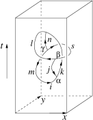
Figure 6: World-lines in a local region represent a local tunneling process, where the topological excitations are created in pairs, and then braided and fused, and at last annihilated in pairs. The picture is also a 2D projection of a 3D string configuration.

A.2 The space-time world lines and quasiparticle tunneling process

In the space-time path integral picture, a “zero law” string operator correspond to a string in a time slice of a fixed time. We can consider more general “zero law” strings in space-time that can go through different times. Those more general strings in space-time correspond to the world-lines of the topological excitations. If the all the world-lines are confined in a local region, then they will represent a local tunneling process, where the topological excitations are created in pairs, and then braided and fused, and at last annihilated in pairs (see Fig. 6). Since the degenerate ground state are locally indistinguishable, such a local tunneling process causes the same amplitude for different degenerate ground states. Thus world-line confined in a local region correspond the a complex number (the amplitude) in the space-time path integral picture. Since the world-line correspond to “zero law” strings, the above complex number (the amplitude) does not depend on the shape and length of the world-line. It only depend on the linking and the fusion of the world lines.

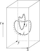
Figure 7: A local tunneling process of two linked world-lines. The dash lines are the framing of the world-lines. In such a tunneling process the framing dash lines do not link with the original strings, indicating that the particles do not twist (or rotate) during the tunneling process. The amplitude of the above linked loops is a complex number denoted as $S^{\text{Lnk}}_{ij}$.

Clearly, number of types of the strings is given by the rank $N$, and the strings are labeled by the simple type $i$ of the topological excitations. Also, the strings are oriented if the particle $i$ and anti-particle $\bar{i}$ are different (see Fig. 7).

The fusion of particles is represented by the branching point of the strings. If $N^{ij}_{k}=0$, then the amplitude of the string configuration that contain a branching point of $i,j,k$ strings will be zero. When $N^{ij}_{k}>1$, it means that the space $i\otimes j$ contain several copies of the space $k$. We will label the copies of the space $k$ by $\alpha=1,2,\cdots,N^{ij}_{k}$. There will be a tunneling amplitude into each copy of the space $k$, and the tunneling amplitude will depend on $\alpha$. So we will include the index $\alpha\in[1,\cdots,N^{ij}_{k}]$ on each branching point. In this case, each such labeled graph of strings gives rise to an amplitude. We will use $A(X)$ to represent such an amplitude for a labeled string configuration $X$, such as the one in Fig. 6.

We also like to mention that the world-lines have a finite cross section which is not circular. So more precisely, the world-lines are represented by framed strings in 7. The framing represents the finite cross section, which do not have rotation symmetry.

A.3 Planar string configurations

In this paper, we will mostly draw the string in 3-dimensional space-time in terms of their projection on a particular plane. In the 2D projected representation, we will always choose a canonical framing, by displacing all the 2D strings a little bit in a direction perpendicular to the 2D plane to obtain the framing dash-lines. So when we draw such 2D string configurations, we will assume the above canonical framing and will not draw the framing dash-lines.

In the rest of this section, we will consider all the amplitudes for planar string configurations, where the strings in the 2D projection do not cross each other. It turns out that the amplitudes for different planar string configurations have a lot of relations, so that we can determine the amplitudes for all the planar string configurations from a set a tensors that satisfy a certain relations. This turns out to be a fusion category theory of the amplitudes for planar string configurations. LABEL:GWW1017 presented such a fusion category theory for more general fermionic case. Here, we will present the simplified case for bosons.

Since the planar string configurations can be viewed as the world line of particles in 1+1D space-time, the fusion category theory described here can also be viewed as the classifying theory for anomalous 1+1D topological orders,Lan and Wen (2014); Kong and Wen (2014); Fiorenza and Valentino (2014) which can be described by the particles tunneling process in 1+1D space-time.

A.4 The first type of linear relations: the F-move

Let us consider a local region in the 2D projected string configuration. We fix all strings cutting across the boundary of the region, and consider all the different ways that the strings connect to each other in the region. Those different string configurations describe different local tunneling process. If a subset of string configurations already describe all the channel of the tunneling processes, then the amplitude of every other local string configuration can be expressed as a linear combination of the amplitudes for the subset of string configurations.

In fact, the graph $\begin{matrix}\includegraphics[scale={.40}]{F1g}\end{matrix}$ with fixed $ijkl$ but different $m\alpha\beta$ is a subset of string configurations that describe all the channel of the local tunneling processes with fixed $ijkl$. The graph $\begin{matrix}\includegraphics[scale={.40}]{F2g}\end{matrix}$ with fixed $ijkl$ but different $n\chi\delta$ is another subset of string configurations that describe all the channel of the local tunneling processes with fixed $ijkl$. So we can express the amplitudes for string configurations in one subset in terms of the amplitudes for string configurations in another subset:

$$A\begin{pmatrix}\includegraphics[scale={.40}]{F1g}\end{pmatrix}=\sum_{n\chi\delta}F^{ijm,i\beta}_{kln,\chi\delta}A\begin{pmatrix}\includegraphics[scale={.40}]{F2g}\end{pmatrix}.$$ (79)

We note that

$$F^{ijm,\alpha\beta}_{kln,\chi\delta}=0\text{ when}$$ (80)

$$N_{ij}^{m}<1\text{ or }N_{mk}^{l}<1\text{ or }N_{jk}^{n}<1\text{ or }N_{in}^{l}<1.$$

When $N^{ij}_{m}<1$ or $N^{mk}_{l}<1$, the left-hand-side of eqn. (79) is always zero. Thus $F^{ijm,\alpha\beta}_{kln,\chi\delta}=0$ when $N^{ij}_{m}<1$ or $N^{mk}_{l}<1$. When $N^{jk}_{n}<1$ or $N^{in}_{l}<1$, amplitude on the right-hand-side of eqn. (79) is always zero. So we can choose $F^{ijm,\alpha\beta}_{kln,\chi\delta}=0$ when $N^{jk}_{n}<1$ or $N^{in}_{l}<1$.

For fixed $i$, $j$, $k$, and $l$, the matrix $F^{ij}_{kl}$ with matrix elements $(F^{ij}_{kl})^{m,\alpha\beta}_{n,\chi\delta}=F^{ijm,\alpha\beta}_{kln,\chi\delta}$ is a matrix of dimension $\sum_{m}N^{ij}_{m}N^{mk}_{l}\times\sum_{n}N^{in}_{l}N^{jk}_{n}$. The matrix describe the relation of the tunneling amplitude through one set of channels described by basis $m\alpha\beta$ and through another set of channels described by basis $n\chi\delta$. We note that the tunneling maps $i,j,k$ to $l$ with degeneracy. The first tunneling path gives rise to basis $m\alpha\beta$ of the degenerate subspace. The second tunneling path gives rise to basis $n\chi\delta$ of the degenerate subspace. The degenerate subspace of $l$ should to the same, regardless the tunneling paths. So we require $N^{ij}_{k}$ to satisfy

$$\sum_{m}N^{ij}_{m}N^{mk}_{l}=\sum_{n}N^{in}_{l}N^{jk}_{n}$$ (81)

and the matrix $F^{ij}_{kl}$ to be unitary:

$$\sum_{n\chi\delta}F^{ijm^{\prime},\alpha^{\prime}\beta^{\prime}}_{kln,\chi\delta}(F^{ijm,\alpha\beta}_{kln,\chi\delta})^{*}=\delta_{m,m^{\prime}}\delta_{\alpha,\alpha^{\prime}}\delta_{\beta,\beta^{\prime}}.$$ (82)

(But here we do not require $N^{ij}_{k}=N^{ji}_{k}$). It is easy to see that the unitary condition implies:

$$A\begin{pmatrix}\includegraphics[scale={.40}]{F2g}\end{pmatrix}=\sum_{m\alpha\beta}\left(F^{ijm,\alpha\beta}_{kln,\chi\delta}\right)^{\dagger}A\begin{pmatrix}\includegraphics[scale={.40}]{F1g}\end{pmatrix}.$$ (83)

Similarly, we have a dual F-move

$$A\begin{pmatrix}\includegraphics[scale={.40}]{F1gD}\end{pmatrix}=\sum_{n\chi\delta}\tilde{F}^{ijm,i\beta}_{kln,\chi\delta}A\begin{pmatrix}\includegraphics[scale={.40}]{F2gD}\end{pmatrix},$$ (84)

where $\tilde{F}^{ijm,i\beta}_{kln,\chi\delta}$ also satisfies a unitary condition.

The F-move (79) can be viewed as a relationship between amplitudes for different graphs that are only differ by a local transformation. Since we can transform one graph to another graph through different paths (i.e. different sets of local F-moves), the F-move (79) must satisfy certain self consistent conditions. For example the graph $\begin{matrix}\includegraphics[scale={.35}]{pent1g}\end{matrix}$ can be transformed to $\begin{matrix}\includegraphics[scale={.35}]{pent3g}\end{matrix}$ through two different paths; one contains two steps of F-moves and another contains three steps of F-moves as described by eqn. (79). The two paths lead to the following relations between the wave functions:

$$A\begin{pmatrix}\includegraphics[scale={.40}]{pent1g}\end{pmatrix} =\sum_{t\eta\varphi}F^{ijm,\alpha\beta}_{knt,\eta\varphi}A\begin{pmatrix}\includegraphics[scale={.40}]{pent4g}\end{pmatrix}=\sum_{t\eta\varphi;s\kappa\gamma}F^{ijm,\alpha\beta}_{knt,\eta\varphi}F^{itn,\varphi\chi}_{lps,\kappa\gamma}A\begin{pmatrix}\includegraphics[scale={.40}]{pent5g}\end{pmatrix}$$

$$=\sum_{t\eta\kappa;\varphi;s\kappa\gamma;q\delta\phi}F^{ijm,\alpha\beta}_{knt,\eta\varphi}F^{itn,\varphi\chi}_{lps,\kappa\gamma}F^{jkt,\eta\kappa}_{lsq,\delta\phi}A\begin{pmatrix}\includegraphics[scale={.40}]{pent3g}\end{pmatrix}.$$ (85)

$$A\begin{pmatrix}\includegraphics[scale={.40}]{pent1g}\end{pmatrix} =\sum_{q\delta\epsilon}F^{mkn,\beta\chi}_{lpq,\delta\epsilon}A\begin{pmatrix}\includegraphics[scale={.40}]{pent2g}\end{pmatrix}=\sum_{q\delta\epsilon;s\phi\gamma}F^{mkn,\beta\chi}_{lpq,\delta\epsilon}F^{ijm,\alpha\epsilon}_{qps,\phi\gamma}A\begin{pmatrix}\includegraphics[scale={.40}]{pent3g}\end{pmatrix},$$ (86)

The consistence of the above two relations leads a condition on the $F$-tensor:

$$\ \ \ \ \sum_{t}\sum_{\eta=1}^{N^{jk}_{t}}\sum_{\varphi=1}^{N^{it}_{n}}\sum_{\kappa=1}^{N^{tl}_{s}}F^{ijm,\alpha\beta}_{knt,\eta\varphi}F^{itn,\varphi\chi}_{lps,\kappa\gamma}F^{jkt,\eta\kappa}_{lsq,\delta\phi}$$

$$=\sum_{\epsilon=1}^{N^{mq}_{p}}F^{mkn,\beta\chi}_{lpq,\delta\epsilon}F^{ijm,\alpha\epsilon}_{qps,\phi\gamma}.$$ (87)

which is the famous pentagon identity. The above pentagon identity (A.4) is a set of nonlinear equations satisfied by the rank-10 tensor $F^{ijm,\alpha\beta}_{kln,\chi\delta}$. The above consistency relations (A.4) are equivalent to the requirement that the local unitary transformations described by eqn. (79) on different paths all commute with each other.

A.5 The second type of linear relations: the O-move

The second type of linear relations re-express the amplitude for $\begin{matrix}\includegraphics[scale={.35}]{iOip}\end{matrix}$ in terms of the amplitude for $\begin{matrix}\includegraphics[scale={.35}]{iline}\end{matrix}$:

$$A\begin{pmatrix}\includegraphics[scale={.40}]{iOip}\end{pmatrix}=O^{jk,\alpha\beta}_{i}\delta_{ii^{\prime}}A\begin{pmatrix}\includegraphics[scale={.40}]{iline}\end{pmatrix}.$$ (88)

We call such local change of graph an O-move. Here $O_{i}^{jk,\alpha\beta}$ satisfies

$$\sum_{k,j}\sum_{\alpha=1}^{N^{jk}_{i}}\sum_{\beta=1}^{N^{jk}_{i}}O^{jk,\alpha\beta}_{i}(O^{jk,\alpha\beta}_{i})^{*}=1$$ (89)

and

$$O^{jk,\alpha\beta}_{i}=0\text{ if } N^{jk}_{i}<1.$$ (90)

We note that the number of choices for the four indices $(j,k,\alpha,\beta)$ in $O_{i}^{jk,\alpha\beta}$ must be equal or greater than $1$:

$$D_{i}=\sum_{jk}(N^{jk}_{i})^{2}\geq 1.$$ (91)

A.6 The third type of linear relations: the Y-move

For fixed $i,j$, $\begin{matrix}\includegraphics[scale={.35}]{ijkY}\end{matrix}$ for different $k\alpha\beta$ describe all the possible tunneling channels. So the amplitude for $\begin{matrix}\includegraphics[scale={.35}]{ij}\end{matrix}$ can be expressed in terms of the amplitudes of $\begin{matrix}\includegraphics[scale={.35}]{ijkY}\end{matrix}$:

$$\sum_{k,\alpha\beta}Y^{ij}_{k,\alpha\beta}A\begin{pmatrix}\includegraphics[scale={.40}]{ijkY}\end{pmatrix}=A\begin{pmatrix}\includegraphics[scale={.40}]{ij}\end{pmatrix}$$ (92)

We will call such a local change as a Y-move. We can choose

$$Y^{ij}_{k,\alpha\beta}=0,\text{ if } N^{ij}_{k}<1.$$ (93)

A.7 A relation between $O_{i}^{jk,{\alpha\beta}}$ and $Y_{k}^{ij,{\alpha\beta}}$

We find that the following tunneling amplitude has two ways of reduction:

$$\sum_{\beta\gamma}Y_{i,{\beta\gamma}}^{jk}A\begin{pmatrix}\includegraphics[scale={.40}]{iOOi}\end{pmatrix} =A\begin{pmatrix}\includegraphics[scale={.40}]{iOi1}\end{pmatrix}$$

$$=O_{i}^{jk,{\alpha\lambda}}A\begin{pmatrix}\includegraphics[scale={.40}]{iline}\end{pmatrix},$$ (94)

$$\ \ \ \ \sum_{\beta\gamma}Y_{i,{\beta\gamma}}^{jk}A\begin{pmatrix}\includegraphics[scale={.40}]{iOOi}\end{pmatrix}$$

$$=\sum_{\beta\gamma}Y_{i,{\beta\gamma}}^{jk}O_{i}^{jk,{\gamma\lambda}}A\begin{pmatrix}\includegraphics[scale={.40}]{iOi}\end{pmatrix}$$

$$=\sum_{\beta\gamma}Y_{i,{\beta\gamma}}^{jk}O_{i}^{jk,{\gamma\lambda}}O_{i}^{jk,{\alpha\beta}}A\begin{pmatrix}\includegraphics[scale={.40}]{iline}\end{pmatrix}$$ (95)

The two reductions should agree, which leads to the condition

$$O_{i}^{jk,{\alpha\lambda}}=\sum_{\beta\gamma}Y_{i,{\beta\gamma}}^{jk}O_{i}^{jk,{\gamma\lambda}}O_{i}^{jk,{\alpha\beta}}$$ (96)

A.8 A freedom of changing basis at each vertex

We note that the following transformation changes the basis at the branching point labeled by $\alpha$

$$A\begin{pmatrix}\includegraphics[scale={.40}]{ijk}\end{pmatrix}\to\sum_{\beta}f^{ij,\alpha}_{k,\beta}A\begin{pmatrix}\includegraphics[scale={.40}]{ijk1}\end{pmatrix},$$ (97)

where $f^{ij}_{k}$ is a unitary matrix

$$\sum_{\beta}f^{ij,\alpha}_{k,\beta}(f^{ij,\alpha^{\prime}}_{k,\beta})^{*}=\delta_{\alpha\lambda^{\prime}}.$$ (98)

Similarly, we have unitary transformation $f^{k,\alpha}_{ij,\beta}$ for vertices with one incoming edges and two outgoing edge. Such transformations correspond to a choice of basis and should be regarded as an equivalent relation.

The above transformation induce the following transformation on $(F^{ijm,\alpha\beta}_{kln,\gamma\lambda}$,$O^{jk,\alpha\beta}_{i}$,$Y_{k,\alpha\beta}^{ij})$:

$$O^{jk,\alpha\beta}_{i} \to f^{i,\alpha}_{jk,\alpha^{\prime}}f^{jk,\beta}_{i,\beta^{\prime}}O^{jk,\alpha^{\prime}\beta^{\prime}}_{i},$$ (99)

$$Y^{ij}_{k,\alpha\beta} \to(f^{ij,\alpha^{\prime}}_{k,\alpha})^{*}(f^{k,\beta^{\prime}}_{ij,\beta})^{*}Y^{ij}_{k,\alpha^{\prime}\beta^{\prime}},$$

$$F^{ijm,\alpha\beta}_{kln,\chi\delta} \to f^{ij,\alpha}_{m,\alpha^{\prime}}f^{mk,\beta}_{l,\beta^{\prime}}(f^{jk,\chi^{\prime}}_{n,\chi})^{*}(f^{in,\delta^{\prime}}_{l,\delta})^{*}F^{ijm,\alpha^{\prime}\beta^{\prime}}_{kln,\chi^{\prime}\delta^{\prime}}.$$

We note that the first line of the above equation is a singular value decomposition, since $f^{i,\alpha}_{jk,\alpha^{\prime}}$ and $f^{jk,\beta}_{i,\beta^{\prime}}$, for fixed $i,j,k$, are independent unitary matrices. Thus, we can use the above basis-changing freedom to choose

$$O^{jk,\alpha\beta}_{i}=O^{jk,\alpha}_{i}\delta_{\alpha\beta},\ \ \ \ O^{jk,\alpha}_{i}\geq 0.$$ (100)

We see that $O^{jk,\alpha}_{i}$, as the singular values, can be chosen to be positive real numbers. Then eqn. (96) implies that

$$Y^{ij}_{k,\alpha\beta}=Y^{ij}_{k,\alpha}\delta_{\alpha\beta},\ \ \ \ Y^{ij}_{k,\alpha}=1/O^{ij,\alpha}_{k}.$$ (101)

A.9 A relation between $O_{i}^{jk,\alpha}$ and $F^{ijm,\alpha\beta}_{kln,\delta\chi}$

We also find another graph that can have two ways of reduction as well:

$$A\begin{pmatrix}\includegraphics[scale={.45}]{iQQi3}\end{pmatrix}=\sum_{s}F^{jkl,\mu\tau}_{mis,\chi\alpha}A\begin{pmatrix}\includegraphics[scale={.45}]{iQQi4}\end{pmatrix}$$

$$=F^{jkl,\mu\tau}_{mip,\chi\alpha}O_{p}^{km,\chi}O_{i}^{jp,\alpha}A\begin{pmatrix}\includegraphics[scale={.45}]{iline}\end{pmatrix}$$ (102)

$$A\begin{pmatrix}\includegraphics[scale={.45}]{iQQi3}\end{pmatrix} =\tilde{F}^{jkl,\mu\tau}_{mip,\chi\alpha}A\begin{pmatrix}\includegraphics[scale={.45}]{iQQi5}\end{pmatrix}$$

$$=\tilde{F}^{jkl,\mu\tau}_{mip,\chi\alpha}O_{l}^{jk,\mu}O_{i}^{lm,\tau}A\begin{pmatrix}\includegraphics[scale={.45}]{iline}\end{pmatrix}$$ (103)

This allows us to obtain another condition

$$\tilde{F}^{jkl,\mu\tau}_{mip,\chi\alpha}=F^{jkl,\mu\tau}_{mip,\chi\alpha}O_{p}^{km,\chi}O_{i}^{jp,\alpha}(O_{i}^{lm,\tau})^{-1}(O_{l}^{jk,\mu})^{-1}$$ (104)

We require $\tilde{F}^{jkl,\mu\tau}_{mip,\chi\alpha}$ to be unitary, which leads to

$$\ \ \ \sum_{l\mu\tau}(F^{jkl,\mu\tau}_{mip^{\prime},\chi^{\prime}\alpha^{\prime}})^{*}\frac{O_{p^{\prime}}^{km,\chi^{\prime}}O_{i}^{jp^{\prime},\alpha^{\prime}}}{O_{i}^{lm,\tau}O_{l}^{jk,\mu}}F^{jkl,\mu\tau}_{mip,\chi\alpha}\frac{O_{p}^{km,\chi}O_{i}^{jp,\alpha}}{O_{i}^{lm,\tau}O_{l}^{jk,\mu}}$$

$$=\sum_{l\mu\tau}\left(F^{jkl,\mu\tau}_{mip^{\prime},\chi^{\prime}\alpha^{\prime}}\right)^{*}F^{jkl,\mu\tau}_{mip,\chi\alpha}\frac{O_{p^{\prime}}^{km,\chi^{\prime}}O_{i}^{jp^{\prime},\alpha^{\prime}}O_{p}^{km,\chi}O_{i}^{jp,\alpha}}{(O_{i}^{lm,\tau}O_{l}^{jk,\mu})^{2}}$$

$$=\delta_{pp^{\prime}}\delta_{\chi\chi^{\prime}}\delta_{\alpha\alpha^{\prime}},$$ (105)

or

$$\sum_{l\mu\tau}\frac{(F^{jkl,\mu\tau}_{mip^{\prime},\chi^{\prime}\alpha^{\prime}})^{*}F^{jkl,\mu\tau}_{mip,\chi\alpha}}{(O_{i}^{lm,\tau}O_{l}^{jk,\mu})^{2}}=\frac{\delta_{pp^{\prime}}\delta_{\chi\chi^{\prime}}\delta_{\alpha\alpha^{\prime}}}{(O_{p}^{km,\chi}O_{i}^{jp,\alpha})^{2}},$$ (106)

The above condition can be satisfied by the following ansatz (note that $O^{ij,\alpha}_{k}$ is real and positive)

$$O^{ij,\alpha}_{k}=\sqrt{\frac{w_{i}w_{j}}{w_{k}}}\delta^{ij}_{k},\ \ \ \ \ \ w_{i}>0,$$ (107)

where $\delta^{jk}_{i}=1$ for $N^{jk}_{i}>0$ and $\delta^{jk}_{i}=0$ for $N^{jk}_{i}=0$. From eqn. (89), we find that $w_{i}$ satisfy

$$\sum_{ij}w_{i}w_{j}N^{ij}_{k}=w_{k}D^{2},\ \ \ D=\sqrt{\sum_{l}w_{l}^{2}}.$$ (108)

The solution of such an equation gives us $w_{i}$.

Let us consider the fusion of $n$ type-$i$ particles. The dimension of the fusion space is

$$D^{i}(n)=\sum_{k_{1},\cdots,k_{n-1}}N^{ik_{n-2}}_{k_{n-1}}\cdots N^{ik_{2}}_{k_{3}}N^{ik_{1}}_{k_{2}}N^{ii}_{k_{1}}$$ (109)

Let $d_{i}$ be the eigenvalue of matrix $N_{i}$ (defined as $(N_{i})_{kj}=N^{ij}_{k}$) with largest absolute value. $d_{i}$ will called quantum dimension of type-$i$ particle. Since all the entry of $N^{ij}_{k}$ are non-negative, one can show that $d_{i}$ is real and positive. We see that the dimension of the fusion space is given by

$$D^{i}(n)=O(1)d_{i}^{n}.$$ (110)

Now, consider $n^{2}$ type-$i$ particles and $n^{2}$ type-$j$ particles. We first fuse $n$ type-$i$ particles, then fuse the result with $n$ type-$j$ particles, and then fuse the result with $n$ type-$i$ particles, etc . The dimension of the fusion space is

$$\sum_{k_{1},\cdots,k_{2n^{2}-1}}\cdots N^{ik_{3n-2}}_{k_{3n-1}}\cdots N^{ik_{2n}}_{k_{2n+1}}N^{ik_{2n-1}}_{k_{2n}}$$

$$\ \ \ \ \ N^{jk_{2n-2}}_{k_{2n-1}}\cdots N^{jk_{n}}_{k_{n+1}}N^{jk_{n-1}}_{k_{n}}N^{ik_{n-2}}_{k_{n-1}}\cdots N^{ik_{1}}_{k_{2}}N^{ii}_{k_{1}}.$$ (111)

The above dimension of the fusion space should be $O(1)d_{i}^{n^{2}}d_{j}^{n^{2}}$. But if the largest-eigenvalue eigenvectors of $N_{i}$ and $N_{j}$ are different, we will get $O(1)d_{i}^{n^{2}}d_{j}^{n^{2}}f^{n}$ as the dimension of the fusion space. The fact that $f=1$ implies that the largest-eigenvalue eigenvectors of $N_{i}$ and $N_{j}$ must be the same (as implied by the condition eqn. (14)). Let $(v_{1},v_{2},\cdots)$ be the common largest-eigenvalue eigenvector for $N_{i}$’s:

$$N_{i}v=d_{i}v.$$ (112)

Since all the entry of $N_{i}$ are non-negative, one can show that $v_{i}$ is real and positive. Using eqn. (14), we find

$$\sum_{m,k}N^{ij}_{m}N^{mk}_{l}v_{k}=\sum_{m,k}N^{im}_{l}N^{jk}_{m}v_{k},$$

$$\sum_{m}N^{ij}_{m}d_{m}v_{l}=d_{i}d_{j}v_{l},\ \ \ d_{i}d_{j}=\sum_{m}N^{ij}_{m}d_{m}.$$ (113)

We see that $d^{T}$ is the left eigenvector of $N_{i}$ with eigenvalue $d_{i}$:

$$d^{T}N_{i}=d^{T}d_{i}.$$ (114)

In other words, the left eigenvector of $N_{i}$ with the largest-eigenvalue is independent of $i$. Such a common left eigenvector is given by $d^{T}$, and the corresponding largest-eigenvalue is the quantum dimension $d_{i}$.

A.10 The fourth type of linear relations: the H-move

Let us consider a new type of move – $H$-move. First, for fixed $i,j,k,l$ $\begin{pmatrix}\includegraphics[scale={.25}]{H1.png}\end{pmatrix}$ and $\begin{pmatrix}\includegraphics[scale={.25}]{H2.png}\end{pmatrix}$ describe all the possible tunneling channels and their can express each other via unitary linear relations:

$$A\begin{pmatrix}\includegraphics[scale={.25}]{H1.png}\end{pmatrix}=\sum_{n\chi\delta}H^{kim,\alpha\beta}_{jln,\chi\delta}A\begin{pmatrix}\includegraphics[scale={.25}]{H2.png}\end{pmatrix}.$$ (115)

In the following, we will show how to compute the coefficients $H^{kim,\alpha\beta}_{jln,\chi\delta}$ from $F^{ijm,\alpha\beta}_{kln,\chi\delta}$ and $w_{i}$.

First, by applying the Y-move, we have:

$$A\begin{pmatrix}\includegraphics[scale={.25}]{H1.png}\end{pmatrix}=\sum_{n,\chi^{\prime}\delta}Y^{kl}_{n,\chi^{\prime}\delta}A\begin{pmatrix}\includegraphics[scale={.25}]{H3.png}\end{pmatrix}.$$ (116)

Next, by applying an inverse F-move, we obtain:

$$A\begin{pmatrix}\includegraphics[scale={.25}]{H3.png}\end{pmatrix}=\sum_{i^{\prime},\beta^{\prime}\chi}{\left(F^{kmi^{\prime},\beta^{\prime}\chi}_{jnl,\beta\chi^{\prime}}\right)}^{\dagger}A\begin{pmatrix}\includegraphics[scale={.25}]{H4.png}\end{pmatrix}.$$ (117)

Finally, by applying the O-move, we end up with:

$$A\begin{pmatrix}\includegraphics[scale={.25}]{H4.png}\end{pmatrix}=O^{km,\alpha\beta^{\prime}}_{i}\delta_{ii^{\prime}}A\begin{pmatrix}\includegraphics[scale={.25}]{H2.png}\end{pmatrix}.$$ (118)

All together, we find:

$$H^{kim,\alpha\beta}_{jln,\chi\delta}=\sum_{\chi^{\prime}\beta^{\prime}}Y^{kl}_{n,\chi^{\prime}\delta}{\left(F^{kmi,\beta^{\prime}\chi}_{jnl,\beta\chi^{\prime}}\right)}^{\dagger}O^{km,\alpha\beta^{\prime}}_{i}$$ (119)

Under the proper basis choice eqn. (100), we can further express the coefficients $H^{ijm,\alpha\beta}_{kln,\chi\delta}$ as:

$$H^{kim,\alpha\beta}_{jln,\chi\delta} =Y^{kl}_{n,\delta}{(F^{kmi,\alpha\chi}_{jnl,\beta\delta})}^{*}O^{km,\alpha}_{i}$$

$$={(F^{kmi,\alpha\chi}_{jnl,\beta\delta})}^{*}{(O^{kl,\delta}_{n})}^{-1}O^{km,\alpha}_{i}$$ (120)

The unitarity condition for H-move requires that:

$$\sum_{n\chi\delta}\frac{F^{km^{\prime}i,\alpha\chi}_{jnl,\beta^{\prime}\delta^{\prime}}{(F^{kmi,\alpha\chi}_{jnl,\beta\delta})}^{*}}{(O^{kl,\delta}_{n})^{2}}=\frac{\delta_{mm^{\prime}}\delta_{\alpha\alpha^{\prime}}\delta_{\beta\beta^{\prime}}}{(O^{km,\alpha}_{i})^{2}},$$ (121)

With the special ansatz eqn. (107), we can further simplify the above two expressions as:

$$H^{kim,\alpha\beta}_{jln,\chi\delta}=\sqrt{\frac{w_{m}w_{n}}{w_{i}w_{l}}}{\left(F^{kmi,\alpha\chi}_{jnl,\beta\delta}\right)}^{*}$$ (122)

and

$$\sum_{n\chi\delta}w_{n}F^{km^{\prime}i,\alpha\chi}_{jnl,\beta^{\prime}\delta^{\prime}}{(F^{kmi,\alpha\chi}_{jnl,\beta\delta})}^{*}=\frac{w_{i}w_{l}}{w_{m}}\delta_{mm^{\prime}}\delta_{\alpha\alpha^{\prime}}\delta_{\beta\beta^{\prime}},$$ (123)

Similarly, we can also construct the dual-H move:

$$A\begin{pmatrix}\includegraphics[scale={.25}]{H5.png}\end{pmatrix}=\sum_{n\chi\delta}\tilde{H}^{kim,\alpha\beta}_{jln,\chi\delta}A\begin{pmatrix}\includegraphics[scale={.25}]{H2.png}\end{pmatrix}.$$ (124)

and we can express $\tilde{H}^{kim,\alpha\beta}_{jln,\chi\delta}$ as:

$$\tilde{H}^{kim,\alpha\beta}_{jln,\chi\delta}=\tilde{H}^{kim,\alpha\beta}_{jln,\chi\delta},$$ (125)

where the coefficients $\tilde{H}^{kim,\alpha\beta}_{jln,\chi\delta}$ can be expressed as:

$$\tilde{H}^{kim,\alpha\beta}_{jln,\chi\delta} =Y^{kl}_{n,\delta}F^{imk,\alpha\delta}_{lnj,\beta\chi}O^{ml,\beta}_{j}$$

$$=F^{imk,\alpha\chi}_{lnj,\beta\delta}{(O^{kl,\delta}_{n})}^{-1}O^{ml,\beta}_{j}$$ (126)

Again, with the special ansatz eqn. (107), we have:

$$\tilde{H}^{kim,\alpha\beta}_{jln,\chi\delta}=\sqrt{\frac{w_{m}w_{n}}{w_{j}w_{k}}}F^{imk,\alpha\delta}_{lnj,\beta\chi}$$ (127)

It is easy to see that the unitarity condition for dual H-move is automatically satisfied if the H-move is unitary.

A.11 Summary of the conditions on the linear relations

We see that valid tunneling amplitudes $A(X)$ can be characterized by tensor data $(N^{ij}_{k},F^{ijm,\alpha\beta}_{kln,\gamma\lambda})$. However, only certain tensor data $(N^{ij}_{k},F^{ijm,\alpha\beta}_{kln,\gamma\lambda})$, that satisfy the conditions eqns. (82, 80, A.4, 108), can self-consistently describe valid tunneling amplitudes $A(X)$.

Those conditions form a set of non-linear equations whose variables are $N^{ij}_{k}$, $F^{ijm,\alpha\beta}_{kln,\gamma\lambda}$, $w_{i}$ (where $w_{i}$ can be determined by $N^{ij}_{k}$ alone). Let us collect those conditions and list them below

$$\bullet\ \sum_{m=0}^{N}N^{ij}_{m}N^{mk}_{l}=\sum_{n=0}^{N}N^{jk}_{n}N^{in}_{l}$$

$$\bullet\ \sum_{jk}(N^{jk}_{i})^{2}\geq 1;$$

$$\bullet\ \sum_{n\chi\delta}F^{ijm^{\prime},\alpha^{\prime}\beta^{\prime}}_{kln,\chi\delta}(F^{ijm,\alpha\beta}_{kln,\chi\delta})^{*}=\delta_{m,m^{\prime}}\delta_{\alpha,\alpha^{\prime}}\delta_{\beta,\beta^{\prime}},$$

$$\bullet\ F^{ijm,\alpha\beta}_{kln,\chi\delta}=0\text{ when}$$

$$\ \ \ \ N^{ij}_{m}<1\text{ or }N^{mk}_{l}<1\text{ or }N^{jk}_{n}<1\text{ or }N^{in}_{l}<1,$$

$$\bullet\ \sum_{t}\sum_{\eta=1}^{N^{jk}_{t}}\sum_{\varphi=1}^{N^{it}_{n}}\sum_{\kappa=1}^{N^{tl}_{s}}F^{ijm,\alpha\beta}_{knt,\eta\varphi}F^{itn,\varphi\chi}_{lps,\kappa\gamma}F^{jkt,\eta\kappa}_{lsq,\delta\phi}$$

$$=\sum_{\epsilon=1}^{N^{mq}_{p}}F^{mkn,\beta\chi}_{lpq,\delta\epsilon}F^{ijm,\alpha\epsilon}_{qps,\phi\gamma}.$$ (129)

$$\bullet\ \sum_{i,j}w_{i}w_{j}N^{ij}_{k}=w_{k}D^{2},\ \ \ D=\sqrt{\sum_{l}w_{l}^{2}}.$$ (130)

$$\bullet\ \sum_{n\chi\delta}w_{n}F^{km^{\prime}i,\alpha\chi}_{jnl,\beta^{\prime}\delta^{\prime}}{(F^{kmi,\alpha\chi}_{jnl,\beta\delta})}^{*}=\frac{w_{i}w_{l}}{w_{m}}\delta_{mm^{\prime}}\delta_{\alpha\alpha^{\prime}}\delta_{\beta\beta^{\prime}},$$ (131)

A.12 A derivation of string fusion algebra

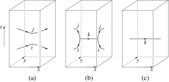
Figure 8: (a): Two tunneling processes: $W^{x}_{i}$ and $W^{x}_{j}$. (b): The tunneling path of the above two tunneling processes can be deformed according to the Y-move (c): The O-move can reduce (b) to (c).

As an application of the above algebraic structure, let us consider the “zero-law” string operators on a torus $S^{1}_{x}\times S^{1}_{y}$, wrapping around the $x$-direction $W^{x}_{i}$. Viewing those string operators as world-lines in space-time, applying the Y-move and then the O-move, and using eqn. (101) (see Fig. 8), we find that

$$W^{x}_{i}W^{x}_{j} =\sum_{k=1}^{N}\sum_{\alpha=1}^{N^{ij}_{k}}Y^{ij}_{k,\alpha}O^{ij,\alpha}_{k}W^{x}_{k}$$

$$=\sum_{k}N^{ij}_{k}W^{x}_{k}.$$ (132)

We see that the algebra of the loop operator $W^{x}_{i}$ forms a representation of fusion algebra $i\otimes j=\sum_{k}N^{ij}_{k}k$. The operators $W^{y}_{i}=SW^{x}_{i}S^{-1}$, where $S$ is the $90^{\circ}$ rotation, satisfy the same fusion algebra

$$W^{y}_{i}W^{y}_{j} =\sum_{k}N^{ij}_{k}W^{y}_{k}.$$ (133)

This way, we derived eqn. (78).

Appendix B Unitary m-fusion category

The tensor data $(N^{ij}_{k},F^{ijm,\alpha\beta}_{kln,\gamma\lambda})$ satisfying the conditions eqns. (A.11), (A.11), (130), and (131) form a so call unitary m-fusion category. In fact, we can view the graph $\begin{matrix}\includegraphics[scale={.40}]{F1g}\end{matrix}$ and the graph $\begin{matrix}\includegraphics[scale={.40}]{F2g}\end{matrix}$ as the different ways to fusion three particle types $i,j,k$ to $N^{ijk}_{l}\equiv\sum_{m}N^{ij}_{m}N^{mk}_{l}=\sum_{m}N^{in}_{l}N^{jk}_{n}$ copies of particles $l$. But the two ways of fusions lead to different basis of the space of $N^{ijk}_{l}$ copies of $l$. The $F^{ijm,\alpha\beta}_{kln,\gamma\lambda}$ tensor is nothing but the unitary transformation that relates the two basis.

However, here we do not require the existence of trivial particles type. Thus the structure we described is not a unitary fusion category. So we call it an unitary m-fusion category (UmFC).

We like to stress that the fusion discussed here is not symmetric (i.e. we do not require $N^{ij}_{k}=N^{ji}_{k}$). Thus fusion that we are talking about is the fusion of 1D particles, where their order cannot be changed. Therefore UmFC is a classifying theory of 1+1D anomalous topological orders ${\cal C}_{1+1}$.Kong and Wen (2014); Lan and Wen (2014) Such anomalous topological orders cannot be realized by any well defined 1D lattice models, but they can realized as boundary of 2D lattice models with non-trivial 2+1D topological orders. Those 2+1D topological orders ${\cal C}_{2+1}$ are described by modular tensor categories, which are uniquely determined by the $1+1D$ anomalous topological order on the boundary. In fact, the 2+1D bulk topological order is the Drinfeld center of the 1+1D anomalous boundary topological order: $C_{2+1}=Z({\cal C}_{1+1})$. One concrete way to compute the Drinfeld center is described in LABEL:LW1384.

Appendix C Unitary fusion category and the trivial particle type

C.1 Trivial particle type and rule of adding trivial strings

In the above discussion, we did not assume the existence of a trivial particle type. Here we will assume such a trivial particle type to exist, and denoted it by $1$, which satisfies the following fusion rule

$$1\otimes i=i\otimes 1=i.$$ (134)

Thus $N^{ij}_{k}$ satisfies

$$N^{1i}_{j}=N^{i1}_{j}=\delta_{ij}.$$ (135)

We also requires that for every $i$ there exists a unique $\bar{i}$ such that

$$\bar{\bar{i}}=i,\ \ \ \bar{1}=1,\ \ \ N^{ij}_{1}=\delta_{i\bar{j}}$$ (136)

By setting $l=1$ in eqn. (14), we find the following symmetry condition on $N^{ij}_{k}$:

$$N_{\bar{k}}^{ij}=N_{\bar{i}}^{jk}.$$ (137)

Using the above, we can rewrite the condition eqn. (130) as

$$\sum_{k}w_{\bar{i}}w_{j}N^{jk}_{i}=w_{\bar{k}}D^{2}.$$ (138)

We see that $w_{\bar{i}}$ is the left eigenvector of $\sum_{j}w_{j}N_{j}$ with eigenvalue $D^{2}$. $D^{2}$ is the largest eigenvalue of $\sum_{j}w_{j}N_{j}$, since the eigenvector has positive elements. As a result $w_{\bar{i}}$ is common left eigenvector of $N_{j}$ for all $j$’s, with eigenvalue $w_{j}$. Since $w_{\bar{i}}$ is non-negative, $w_{j}$ is the largest eigenvalue of $N_{j}$. Therefore

$$w_{j}=d_{j}$$ (139)

is the quantum dimension of type-$j$ particle (see eqn. (114)). The largest left eigenvalue of $N_{1}$ is 1. Thus $d_{1}=w_{1}=1$.

We can represent a type-$1$ string by a dash line. By examine the O-move with $k=1$:

$$A\begin{pmatrix}\includegraphics[scale={.40}]{iOdi}\end{pmatrix}=A\begin{pmatrix}\includegraphics[scale={.40}]{iline}\end{pmatrix}.$$ (140)

we see that we can remove or add any vertex with dash line without affecting the amplitude. In other words, a vertex with dash line can be added/removed freely. The unitary m-fusion categories with the trivial particle type will be called unitary fusion categories.

C.2 Amplitudes for loops

Figure 9: A loop of type-$i$ string has an amplitude $d_{i}$.

The tensors $N^{ij}_{k}$, $F^{ijm,\alpha\beta}_{kln,\gamma\lambda}$ characterize the four types of linear relations between graphs with some local differences. Those local changes are almost complete, in the sense that any graphs of strings can be reduce to graphs that contain only isolated loops. Since the amplitude of a graph that contain disconnect parts is given by the product of the amplitudes for those parts, therefore, if we know the amplitude for single loops of string, then the amplitude of any string configuration can be computed from the tensor data $(N^{ij}_{k},F^{ijm,\alpha\beta}_{kln,\gamma\lambda})$.

With the presence of trivial particle type in the unitary fusion category, we can determine the amplitude for a loop of $i$-string. Using the rule of adding dash lines (the trivial strings) and $O$-move eqn. (107), we find

$$A\begin{pmatrix}\includegraphics[scale={.40}]{ilp}\end{pmatrix} =A\begin{pmatrix}\includegraphics[scale={.40}]{ilp1lp}\end{pmatrix}=O^{i\bar{i}}_{1}A\begin{pmatrix}\includegraphics[scale={.40}]{1lp}\end{pmatrix}$$

$$=d_{i}A\begin{pmatrix}\includegraphics[scale={.40}]{1lp}\end{pmatrix}$$ (141)

We may choose $A\begin{pmatrix}\includegraphics[scale={.40}]{1lp}\end{pmatrix}=1$. This allows we to determine (see Fig. 9)

$$A\begin{pmatrix}\includegraphics[scale={.40}]{ilp}\end{pmatrix}=d_{i}.$$ (142)

Appendix D Modular tensor category for the amplitudes of non-planar string configurations

D.1 Commutative unitary fusion category

We have being considering planar graphs and the related fusion category theory. In this section we will consider non-planar graphs. Since the particles now live in 2D space, the fusion of the particles satisfies

$$i\otimes j=j\otimes i,$$ (143)

and thus

$$N^{ij}_{k}=N^{ji}_{k}.$$ (144)

So the fusion of 2D particles are commutative (while the fusion of 1D particles may not be commutative). The fusion with $N^{ij}_{k}=N^{ji}_{k}$ is called commutative. Also, we assume the existence of trivial particle type. Thus, in this section, the fusion of the particles is described by a commutative unitary fusion category.

The commutative unitary fusion category for planar graphs plus the extra structure for non-planar graphs and their amplitudes will give us a modular tensor category theory. In this section, we will derive many conditions that involve amplitudes of non-planar graphs.

D.2 Amplitude for linked loops and Verlinde formula

Figure 10: A Y-move can change a linking of three loops in (a) to two linkings of two loops in (b). The amplitude for two linked $i$-loop and $l$-loop in (c) is denoted as $S^{\text{Lnk}}_{il}$.

As the first application of non-planar graphs, consider a three linked loops in Fig. 10a. We can evaluate the graph in two ways: (a) we fuse the $i$-loop and $j$-loop using eqn. (78) to produce a single $k$-loop; (b) we use a Y-move to change the linking of three loops to two linkings of two loops. We defined the amplitude for two linked loops $i$ and $j$ as $S^{\text{Lnk}}_{ij}$ (see Fig. 7). $S^{\text{Lnk}}_{ij}$ satisfies

$$S^{\text{Lnk}}_{ij}=S^{\text{Lnk}}_{ji}.$$ (145)

This allows us to obtain

$$\sum_{k}N^{ij}_{k}S^{\text{Lnk}}_{kl}=Y^{\bar{l}l}_{1}S^{\text{Lnk}}_{il}S^{\text{Lnk}}_{jl}=\frac{S^{\text{Lnk}}_{il}S^{\text{Lnk}}_{jl}}{d_{l}},$$ (146)

which is the tensor category version of Verlinde formula.

D.3 Degenerate ground states on torus and excitation basis

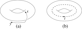
Figure 11: (a): The ground state $|1\rangle$ on a torus that corresponds to the trivial quasiparticle can be represented by an empty solid torus. (b): The other ground state $|i\rangle$ that corresponds to a type $i$ quasiparticle can be represented by an solid torus with a loop of type $i$ in the center.

Figure 12: The graphic representation of $W^{x}_{j}|i\rangle$.

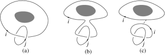
Figure 13: (a): The graphic representation of $W^{x}_{j}|i\rangle$. (b): The graphic representation of $W^{x}_{j}|i\rangle$. (c): The Y-move can deformed the graph in (b) to the graph in (c). The shaded area represents the hole of the torus.

To obtain the algebraic structure for non-planar graphs, let us first try to represent the degenerate ground states on torus graphically. One of the degenerate ground state that corresponds to the trivial quasiparticle $i=1$ can be represented by an empty solid torus $S^{1}_{x}\times D^{2}_{yt}$ (see Fig. 11a), where the circle in $y$-direction $S^{1}_{y}$ is a boundary of the disk $D^{2}_{yt}$. In other words, the path integral on the space-time $S^{1}_{x}\times D^{2}_{yt}$ give rise to the state $|1\rangle$ on the surface $S^{1}_{x}\times S^{1}_{y}$. We denote such a state as $|1\rangle$. Other degenerated ground states can be obtained by the action of the $W^{y}_{i}$ operators

$$|i\rangle\equiv W^{y}_{i}|1\rangle.$$ (147)

$|i\rangle$’s form a orthonormal basis if we assume $(W^{y}_{i})^{\dagger}=W^{y}_{\bar{i}}$ and $\langle i|1\rangle=\delta_{i1}$. This is because

$$\langle j|i\rangle =\langle 1|=\langle 1|W^{y}_{\bar{j}}W^{y}_{i}|1\rangle=\langle 1|\sum_{k}N^{\bar{j}i}_{k}W^{y}_{k}|1\rangle$$

$$=\langle 1|N^{\bar{j}i}_{1}|1\rangle=\delta_{ij}$$ (148)

We will call such a basis of the degenerate ground state an excitation basis.

Since $|i\rangle$ is created by the tunneling operator $W^{y}_{i}$, $|i\rangle$ can be represented by adding a $i$-loop that corresponds to the $W^{y}_{i}$ operator to the center of the solid torus (see Fig. 11b).

$|i\rangle$ is a natural basis, where the matrix elements of $W^{x}_{l}$ and $W^{y}_{l}$ have simple forms. From eqn. (133), we see that

$$W^{y}_{j}W^{y}_{i}|1\rangle =W^{y}_{j}|i\rangle=\sum_{k}N^{ji}_{k}|k\rangle.$$ (149)

The action of $W^{x}_{j}$ on $|i\rangle$ is represented by Fig. 12. From Fig. 13, we find that

$$W^{x}_{j}|i\rangle=Y^{\bar{i}i}_{1}S^{\text{Lnk}}_{ij}|i\rangle=\frac{S^{\text{Lnk}}_{ij}}{d_{i}}|i\rangle.$$ (150)

We see that $|i\rangle$’s are common eigenstates of the commuting set of operators $W^{x}_{j}$. The corresponding eigenvalue for $W^{x}_{j}$ is $\frac{S^{\text{Lnk}}_{ij}}{d_{i}}$. We see that different $|i\rangle$’s have different set of eigenvalues, which support our assumption $\langle i|1\rangle=\delta_{i1}$.

Table 11: A list of primitive bosonic topological orders (up to invertible ones) in 2+1D with rank $N=2,3,\cdots,6$. The list contain all topological orders with rank $N=2,3,4$. The list may not be complete for rank $N=5,6$. However, it contains all rank $N=5$ primitive topological orders (i.e. UMTC’s) with $D^{2}\leq 120$, and all rank $N=6$ primitive topological orders (i.e. UMTC’s) with $D^{2}\leq 101$.

$N^{B}_{c}$	$S_{\text{top}}$	$D^{2}$	$d_{1},d_{2},\cdots$	$s_{1},s_{2},\cdots$	$K$-matrix/SCA
$2_{1}^{B}$	$0.5$	$2$	$1,1$	$0,\frac{1}{4}$	$(2)$
$2_{-1}^{B}$	$0.5$	$2$	$1,1$	$0,-\frac{1}{4}$	$(-2)$
$2_{14/5}^{B}$	$0.9276$	$3.6180$	$1,\zeta_{3}^{1}$	$0,\frac{2}{5}$	$(A_{1},3)_{1/2},\ (G_{2},1)$
$2_{-14/5}^{B}$	$0.9276$	$3.6180$	$1,\zeta_{3}^{1}$	$0,-\frac{2}{5}$	$(A_{1},-3)_{1/2},\ (G_{2},-1)$
$3_{2}^{B}$	$0.7924$	$3$	$1,1,1$	$0,\frac{1}{3},\frac{1}{3}$	$(2\ 2;1)$
$3_{-2}^{B}$	$0.7924$	$3$	$1,1,1$	$0,-\frac{1}{3},-\frac{1}{3}$	$-(2\ 2;1)$
$3_{3/2}^{B}$	$1$	$4$	$1,1,\sqrt{2}$	$0,\frac{1}{2},\frac{3}{16}$	$(A_{1},2),(B_{9},1)$
$3_{5/2}^{B}$	$1$	$4$	$1,1,\sqrt{2}$	$0,\frac{1}{2},\frac{5}{16}$	$(B_{2},1)$
$3_{7/2}^{B}$	$1$	$4$	$1,1,\sqrt{2}$	$0,\frac{1}{2},\frac{7}{16}$	$(B_{3},1)$
$3_{-7/2}^{B}$	$1$	$4$	$1,1,\sqrt{2}$	$0,\frac{1}{2},-\frac{7}{16}$	$(B_{4},1)$
$3_{-5/2}^{B}$	$1$	$4$	$1,1,\sqrt{2}$	$0,\frac{1}{2},-\frac{5}{16}$	$(B_{5},1)$
$3_{-3/2}^{B}$	$1$	$4$	$1,1,\sqrt{2}$	$0,\frac{1}{2},-\frac{3}{16}$	$(B_{6},1)$
$3_{-1/2}^{B}$	$1$	$4$	$1,1,\sqrt{2}$	$0,\frac{1}{2},-\frac{1}{16}$	$(B_{7},1)$
$3_{1/2}^{B}$	$1$	$4$	$1,1,\sqrt{2}$	$0,\frac{1}{2},\frac{1}{16}$	$(B_{8},1)$
$3_{8/7}^{B}$	$1.6082$	$9.2958$	$1,\zeta_{5}^{1},\zeta_{5}^{2}$	$0,-\frac{1}{7},\frac{2}{7}$	$(A_{1},5)_{1/2}$
$3_{-8/7}^{B}$	$1.6082$	$9.2958$	$1,\zeta_{5}^{1},\zeta_{5}^{2}$	$0,\frac{1}{7},-\frac{2}{7}$	$(A_{1},-5)_{1/2}$
$4_{0}^{B}$	$1$	$4$	$1,1,1,1$	$0,0,0,\frac{1}{2}$	$(0,0;2)$
$4_{1}^{B}$	$1$	$4$	$1,1,1,1$	$0,\frac{1}{8},\frac{1}{8},\frac{1}{2}$	$(4)$
$4_{-1}^{B}$	$1$	$4$	$1,1,1,1$	$0,-\frac{1}{8},-\frac{1}{8},\frac{1}{2}$	$(-4)$
$4_{3}^{B}$	$1$	$4$	$1,1,1,1$	$0,\frac{3}{8},\frac{3}{8},\frac{1}{2}$	$(2\ 2\ 2;1\ 1;1)$
$4_{-3}^{B}$	$1$	$4$	$1,1,1,1$	$0,-\frac{3}{8},-\frac{3}{8},\frac{1}{2}$	$-(2\ 2\ 2;1\ 1;1)$
$4_{4}^{B}$	$1$	$4$	$1,1,1,1$	$0,\frac{1}{2},\frac{1}{2},\frac{1}{2}$	$(2\ 2\ 2\ 2;1\ 0\ 0;1\ 0;1)$
$4_{10/3}^{B}$	$2.1328$	$19.234$	$1,\zeta_{7}^{1},\zeta_{7}^{2},\zeta_{7}^{3}$	$0,\frac{1}{3},\frac{2}{9},-\frac{1}{3}$	$(A_{1},7)_{1/2}$
$4_{-10/3}^{B}$	$2.1328$	$19.234$	$1,\zeta_{7}^{1},\zeta_{7}^{2},\zeta_{7}^{3}$	$0,-\frac{1}{3},-\frac{2}{9},\frac{1}{3}$	$(A_{1},-7)_{1/2},(G_{2},2)$
$5_{0}^{B}$	$1.1609$	$5$	$1,1,1,1,1$	$0,\frac{1}{5},\frac{1}{5},-\frac{1}{5},-\frac{1}{5}$	$(2\ 2;3)$
$5_{4}^{B}$	$1.1609$	$5$	$1,1,1,1,1$	$0,\frac{2}{5},\frac{2}{5},-\frac{2}{5},-\frac{2}{5}$	$(2\ 2\ 2\ 2;1\ 1\ 0;1\ 0;1)$
$5_{2}^{B,a}$	$1.7924$	$12$	$1,1,\sqrt{3},\sqrt{3},2$	$0,0,\frac{1}{8},-\frac{3}{8},\frac{1}{3}$	$(A_{1},4)$
$5_{2}^{B,b}$	$1.7924$	$12$	$1,1,\sqrt{3},\sqrt{3},2$	$0,0,-\frac{1}{8},\frac{3}{8},\frac{1}{3}$	$(5_{2}^{B,a}\boxtimes 2_{1}^{B}\boxtimes 2_{-1}^{B})_{1/4}$
$5_{-2}^{B,a}$	$1.7924$	$12$	$1,1,\sqrt{3},\sqrt{3},2$	$0,0,-\frac{1}{8},\frac{3}{8},-\frac{1}{3}$	$(A_{1},-4)$
$5_{-2}^{B,b}$	$1.7924$	$12$	$1,1,\sqrt{3},\sqrt{3},2$	$0,0,\frac{1}{8},-\frac{3}{8},-\frac{1}{3}$	$(5_{-2}^{B,a}\boxtimes 2_{1}^{B}\boxtimes 2_{-1}^{B})_{1/4}$
$5_{16/11}^{B}$	$2.5573$	$34.646$	$1,\zeta_{9}^{1},\zeta_{9}^{2},\zeta_{9}^{3},\zeta_{9}^{4}$	$0,-\frac{2}{11},\frac{2}{11},\frac{1}{11},-\frac{5}{11}$	$(A_{1},9)_{1/2},\ (F_{4},2)$
$5_{-16/11}^{B}$	$2.5573$	$34.646$	$1,\zeta_{9}^{1},\zeta_{9}^{2},\zeta_{9}^{3},\zeta_{9}^{4}$	$0,\frac{2}{11},-\frac{2}{11},-\frac{1}{11},\frac{5}{11}$	$(A_{1},-9)_{1/2},\ (E_{8},3)$
$5_{18/7}^{B}$	$2.5716$	$35.342$	$1,\frac{1}{2}\zeta_{12}^{6},\frac{1}{2}\zeta_{12}^{6},\zeta_{12}^{2},\zeta_{12}^{4}$	$0,-\frac{1}{7},-\frac{1}{7},\frac{1}{7},\frac{3}{7}$	$(A_{1},12)_{1/4},\ (A_{2},4)_{1/3}$
$5_{-18/7}^{B}$	$2.5716$	$35.342$	$1,\frac{1}{2}\zeta_{12}^{6},\frac{1}{2}\zeta_{12}^{2},\zeta_{12}^{2},\zeta_{12}^{4}$	$0,\frac{1}{7},\frac{1}{7},-\frac{1}{7},-\frac{3}{7}$	$(A_{3},3)_{1/4}$
$6_{0}^{B,a}$	$2.1609$	$20$	$1,1,2,2,\sqrt{5},\sqrt{5}$	$0,0,\frac{1}{5},-\frac{1}{5},0,\frac{1}{2}$	$(D_{5},2)_{1/4},\ (U(1)_{5}/\mathbb{Z}_{2})_{1/2}$
$6_{0}^{B,b}$	$2.1609$	$20$	$1,1,2,2,\sqrt{5},\sqrt{5}$	$0,0,\frac{1}{5},-\frac{1}{5},\frac{1}{4},-\frac{1}{4}$	$(6_{0}^{B,a}\boxtimes 2_{1}^{B}\boxtimes 2_{-1}^{B})_{1/4}$
$6_{4}^{B,a}$	$2.1609$	$20$	$1,1,2,2,\sqrt{5},\sqrt{5}$	$0,0,\frac{2}{5},-\frac{2}{5},\frac{1}{4},-\frac{1}{4}$	$(B_{2},2)$
$6_{4}^{B,b}$	$2.1609$	$20$	$1,1,2,2,\sqrt{5},\sqrt{5}$	$0,0,\frac{2}{5},-\frac{2}{5},0,\frac{1}{2}$	$(6_{4}^{B,a}\boxtimes 2_{1}^{B}\boxtimes 2_{-1}^{B})_{1/4}$
$6_{46/13}^{B}$	$2.9132$	$56.746$	$1,\zeta_{11}^{1},\zeta_{11}^{2},\zeta_{11}^{3},\zeta_{11}^{4},\zeta_{11}^{5}$	$0,\frac{4}{13},\frac{2}{13},-\frac{6}{13},\frac{6}{13},-\frac{1}{13}$	$(A_{1},11)_{1/2}$
$6_{-46/13}^{B}$	$2.9132$	$56.746$	$1,\zeta_{11}^{1},\zeta_{11}^{2},\zeta_{11}^{3},\zeta_{11}^{4},\zeta_{11}^{5}$	$0,-\frac{4}{13},-\frac{2}{13},\frac{6}{13},-\frac{6}{13},\frac{1}{13}$	$(A_{1},-11)_{1/2}$
$6_{8/3}^{B}$	$3.1107$	$74.617$	$1,\frac{1}{2}\zeta_{16}^{8},\frac{1}{2}\zeta_{16}^{8},\zeta_{16}^{2},\zeta_{16}^{4},\zeta_{16}^{6}$	$0,\frac{1}{9},\frac{1}{9},\frac{1}{9},\frac{1}{3},-\frac{1}{3}$	$(A_{1},16)_{1/4}$
$6_{-8/3}^{B}$	$3.1107$	$74.617$	$1,\frac{1}{2}\zeta_{16}^{8},\frac{1}{2}\zeta_{16}^{8},\zeta_{16}^{2},\zeta_{16}^{4},\zeta_{16}^{6}$	$0,-\frac{1}{9},-\frac{1}{9},-\frac{1}{9},-\frac{1}{3},\frac{1}{3}$	$(A_{1},-16)_{1/4},\ (A_{2},6)_{1/9}$
$6_{2}^{B}$	$3.3263$	$100.61$	$1,\frac{3+\sqrt{21}}{2},\frac{3+\sqrt{21}}{2},\frac{3+\sqrt{21}}{2},\frac{5+\sqrt{21}}{2},\frac{7+\sqrt{21}}{2}$	$0,-\frac{1}{7},-\frac{2}{7},\frac{3}{7},0,\frac{1}{3}$	$(G_{2},-3)$
$6_{-2}^{B}$	$3.3263$	$100.61$	$1,\frac{3+\sqrt{21}}{2},\frac{3+\sqrt{21}}{2},\frac{3+\sqrt{21}}{2},\frac{5+\sqrt{21}}{2},\frac{7+\sqrt{21}}{2}$	$0,\frac{1}{7},\frac{2}{7},-\frac{3}{7},0,-\frac{1}{3}$	$(G_{2},3)$

Table 12: A list of primitive bosonic topological orders (up to invertible ones) in 2+1D with rank $N=7,8,9$. The list may not be complete. However, it contains all rank $N=7$ primitive topological orders (i.e. UMTC’s) with $D^{2}\leq 40$, all rank $N=8$ primitive topological orders with $D^{2}\leq 25$, and all rank $N=9$ primitive topological orders with $D^{2}\leq 20$.

$N^{B}_{c}$	$S_{\text{top}}$	$D^{2}$	$d_{1},d_{2},\cdots$	$s_{1},s_{2},\cdots$	$K$-matrix/SCA
$7_{2}^{B,a}$	$1.4036$	$7$	$1,1,1,1,1,1,1$	$0,\frac{1}{7},\frac{1}{7},\frac{2}{7},\frac{2}{7},-\frac{3}{7},-\frac{3}{7}$	$(4\ 4;3)$
$7_{-2}^{B,a}$	$1.4036$	$7$	$1,1,1,1,1,1,1$	$0,-\frac{1}{7},-\frac{1}{7},-\frac{2}{7},-\frac{2}{7},\frac{3}{7},\frac{3}{7}$	$-(4\ 4;3),\ (A_{6},1)$
$7_{9/4}^{B}$	$2.3857$	$27.313$	$1,1,\zeta_{6}^{1},\zeta_{6}^{1},\zeta_{6}^{2},\zeta_{6}^{2},\zeta_{6}^{3}$	$0,\frac{1}{2},\frac{3}{32},\frac{3}{32},\frac{1}{4},-\frac{1}{4},\frac{15}{32}$	$(A_{1},6)$
$7_{13/4}^{B}$	$2.3857$	$27.313$	$1,1,\zeta_{6}^{1},\zeta_{6}^{1},\zeta_{6}^{2},\zeta_{6}^{2},\zeta_{6}^{3}$	$0,\frac{1}{2},\frac{7}{32},\frac{7}{32},\frac{1}{4},-\frac{1}{4},-\frac{13}{32}$	$(7_{9/4}^{B}\boxtimes 4_{1}^{B})_{1/4}$
$7_{-15/4}^{B}$	$2.3857$	$27.313$	$1,1,\zeta_{6}^{1},\zeta_{6}^{1},\zeta_{6}^{2},\zeta_{6}^{2},\zeta_{6}^{3}$	$0,\frac{1}{2},\frac{11}{32},\frac{11}{32},\frac{1}{4},-\frac{1}{4},-\frac{9}{32}$	$(7_{13/4}^{B}\boxtimes 4_{1}^{B})_{1/4}$
$7_{-11/4}^{B}$	$2.3857$	$27.313$	$1,1,\zeta_{6}^{1},\zeta_{6}^{1},\zeta_{6}^{2},\zeta_{6}^{2},\zeta_{6}^{3}$	$0,\frac{1}{2},\frac{15}{32},\frac{15}{32},\frac{1}{4},-\frac{1}{4},-\frac{5}{32}$	$(7_{-15/4}^{B}\boxtimes 4_{1}^{B})_{1/4}$
$7_{-7/4}^{B}$	$2.3857$	$27.313$	$1,1,\zeta_{6}^{1},\zeta_{6}^{1},\zeta_{6}^{2},\zeta_{6}^{2},\zeta_{6}^{3}$	$0,\frac{1}{2},-\frac{13}{32},-\frac{13}{32},\frac{1}{4},-\frac{1}{4},-\frac{1}{32}$	$(7_{-11/4}^{B}\boxtimes 4_{1}^{B})_{1/4}$
$7_{-3/4}^{B}$	$2.3857$	$27.313$	$1,1,\zeta_{6}^{1},\zeta_{6}^{1},\zeta_{6}^{2},\zeta_{6}^{2},\zeta_{6}^{3}$	$0,\frac{1}{2},-\frac{9}{32},-\frac{9}{32},\frac{1}{4},-\frac{1}{4},\frac{3}{32}$	$(7_{-7/4}^{B}\boxtimes 4_{1}^{B})_{1/4}$
$7_{1/4}^{B}$	$2.3857$	$27.313$	$1,1,\zeta_{6}^{1},\zeta_{6}^{1},\zeta_{6}^{2},\zeta_{6}^{2},\zeta_{6}^{3}$	$0,\frac{1}{2},-\frac{5}{32},-\frac{5}{32},\frac{1}{4},-\frac{1}{4},\frac{7}{32}$	$(7_{-3/4}^{B}\boxtimes 4_{1}^{B})_{1/4}$
$7_{5/4}^{B}$	$2.3857$	$27.313$	$1,1,\zeta_{6}^{1},\zeta_{6}^{1},\zeta_{6}^{2},\zeta_{6}^{2},\zeta_{6}^{3}$	$0,\frac{1}{2},-\frac{1}{32},-\frac{1}{32},\frac{1}{4},-\frac{1}{4},\frac{11}{32}$	$(7_{1/4}^{B}\boxtimes 4_{1}^{B})_{1/4}$
$7_{7/4}^{B}$	$2.3857$	$27.313$	$1,1,\zeta_{6}^{1},\zeta_{6}^{1},\zeta_{6}^{2},\zeta_{6}^{2},\zeta_{6}^{3}$	$0,\frac{1}{2},\frac{13}{32},\frac{13}{32},\frac{1}{4},-\frac{1}{4},\frac{1}{32}$	$(C_{6},1)$
$7_{11/4}^{B}$	$2.3857$	$27.313$	$1,1,\zeta_{6}^{1},\zeta_{6}^{1},\zeta_{6}^{2},\zeta_{6}^{2},\zeta_{6}^{3}$	$0,\frac{1}{2},-\frac{15}{32},-\frac{15}{32},\frac{1}{4},-\frac{1}{4},\frac{5}{32}$	$(7_{7/4}^{B}\boxtimes 4_{1}^{B})_{1/4}$
$7_{15/4}^{B}$	$2.3857$	$27.313$	$1,1,\zeta_{6}^{1},\zeta_{6}^{1},\zeta_{6}^{2},\zeta_{6}^{2},\zeta_{6}^{3}$	$0,\frac{1}{2},-\frac{11}{32},-\frac{11}{32},\frac{1}{4},-\frac{1}{4},\frac{9}{32}$	$(7_{11/4}^{B}\boxtimes 4_{1}^{B})_{1/4}$
$7_{-13/4}^{B}$	$2.3857$	$27.313$	$1,1,\zeta_{6}^{1},\zeta_{6}^{1},\zeta_{6}^{2},\zeta_{6}^{2},\zeta_{6}^{3}$	$0,\frac{1}{2},-\frac{7}{32},-\frac{7}{32},\frac{1}{4},-\frac{1}{4},\frac{13}{32}$	$(7_{15/4}^{B}\boxtimes 4_{1}^{B})_{1/4}$
$7_{-9/4}^{B}$	$2.3857$	$27.313$	$1,1,\zeta_{6}^{1},\zeta_{6}^{1},\zeta_{6}^{2},\zeta_{6}^{2},\zeta_{6}^{3}$	$0,\frac{1}{2},-\frac{3}{32},-\frac{3}{32},\frac{1}{4},-\frac{1}{4},-\frac{15}{32}$	$(7_{-13/4}^{B}\boxtimes 4_{1}^{B})_{1/4}$
$7_{-5/4}^{B}$	$2.3857$	$27.313$	$1,1,\zeta_{6}^{1},\zeta_{6}^{1},\zeta_{6}^{2},\zeta_{6}^{2},\zeta_{6}^{3}$	$0,\frac{1}{2},\frac{1}{32},\frac{1}{32},\frac{1}{4},-\frac{1}{4},-\frac{11}{32}$	$(7_{-9/4}^{B}\boxtimes 4_{1}^{B})_{1/4}$
$7_{-1/4}^{B}$	$2.3857$	$27.313$	$1,1,\zeta_{6}^{1},\zeta_{6}^{1},\zeta_{6}^{2},\zeta_{6}^{2},\zeta_{6}^{3}$	$0,\frac{1}{2},\frac{5}{32},\frac{5}{32},\frac{1}{4},-\frac{1}{4},-\frac{7}{32}$	$(7_{-5/4}^{B}\boxtimes 4_{1}^{B})_{1/4}$
$7_{3/4}^{B}$	$2.3857$	$27.313$	$1,1,\zeta_{6}^{1},\zeta_{6}^{1},\zeta_{6}^{2},\zeta_{6}^{2},\zeta_{6}^{3}$	$0,\frac{1}{2},\frac{9}{32},\frac{9}{32},\frac{1}{4},-\frac{1}{4},-\frac{3}{32}$	$(7_{-1/4}^{B}\boxtimes 4_{1}^{B})_{1/4}$
$7_{2}^{B,b}$	$2.4036$	$28$	$1,1,2,2,2,\sqrt{7},\sqrt{7}$	$0,0,\frac{1}{7},\frac{2}{7},-\frac{3}{7},\frac{1}{8},-\frac{3}{8}$	$(U(1)_{7}/\mathbb{Z}_{2})_{1/2}$
$7_{2}^{B,c}$	$2.4036$	$28$	$1,1,2,2,2,\sqrt{7},\sqrt{7}$	$0,0,\frac{1}{7},\frac{2}{7},-\frac{3}{7},-\frac{1}{8},\frac{3}{8}$	$(7_{2}^{B,b}\boxtimes 2_{1}^{B}\boxtimes 2_{-1}^{B})_{1/4}$
$7_{-2}^{B,b}$	$2.4036$	$28$	$1,1,2,2,2,\sqrt{7},\sqrt{7}$	$0,0,-\frac{1}{7},-\frac{2}{7},\frac{3}{7},-\frac{1}{8},\frac{3}{8}$	$(B_{3},2),\ (D_{7},2)_{1/2}$
$7_{-2}^{B,c}$	$2.4036$	$28$	$1,1,2,2,2,\sqrt{7},\sqrt{7}$	$0,0,-\frac{1}{7},-\frac{2}{7},\frac{3}{7},\frac{1}{8},-\frac{3}{8}$	$(7_{-2}^{B,b}\boxtimes 2_{1}^{B}\boxtimes 2_{-1}^{B})_{1/4}$
$7_{8/5}^{B}$	$3.2194$	$86.750$	$1,\zeta_{13}^{1},\zeta_{13}^{2},\zeta_{13}^{3},\zeta_{13}^{4},\zeta_{13}^{5},\zeta_{13}^{6}$	$0,-\frac{1}{5},\frac{2}{15},0,\frac{2}{5},\frac{1}{3},-\frac{1}{5}$	$(A_{1},13)_{1/2}$
$7_{-8/5}^{B}$	$3.2194$	$86.750$	$1,\zeta_{13}^{1},\zeta_{13}^{2},\zeta_{13}^{3},\zeta_{13}^{4},\zeta_{13}^{5},\zeta_{13}^{6}$	$0,\frac{1}{5},-\frac{2}{15},0,-\frac{2}{5},-\frac{1}{3},\frac{1}{5}$	$(A_{1},-13)_{1/2}$
$7_{1}^{B}$	$3.2715$	$93.254$	$1,\zeta_{6}^{2},\zeta_{6}^{2},1+\zeta_{6}^{2},1+\zeta_{6}^{2},2\zeta_{6}^{2},1+2\zeta_{6}^{2}$	$0,\frac{1}{2},\frac{1}{2},\frac{1}{4},\frac{1}{4},-\frac{3}{8},0$	$(A_{2},5)_{1/3}$
$7_{-1}^{B}$	$3.2715$	$93.254$	$1,\zeta_{6}^{2},\zeta_{6}^{2},1+\zeta_{6}^{2},1+\zeta_{6}^{2},2\zeta_{6}^{2},1+2\zeta_{6}^{2}$	$0,\frac{1}{2},\frac{1}{2},-\frac{1}{4},-\frac{1}{4},\frac{3}{8},0$	$(A_{2},-5)_{1/3}$
$7_{30/11}^{B}$	$3.5425$	$135.77$	$1,\zeta_{20}^{2},\frac{1}{2}\zeta_{20}^{10},\frac{1}{2}\zeta_{20}^{10},\zeta_{20}^{4},\zeta_{20}^{6},\zeta_{20}^{8}$	$0,\frac{1}{11},\frac{4}{11},\frac{4}{11},\frac{3}{11},-\frac{5}{11},-\frac{1}{11}$	$(A_{1},20)_{1/4}$
$7_{-30/11}^{B}$	$3.5425$	$135.77$	$1,\zeta_{20}^{2},\frac{1}{2}\zeta_{20}^{10},\frac{1}{2}\zeta_{20}^{10},\zeta_{20}^{4},\zeta_{20}^{6},\zeta_{20}^{8}$	$0,-\frac{1}{11},-\frac{4}{11},-\frac{4}{11},-\frac{3}{11},\frac{5}{11},\frac{1}{11}$	$(A_{1},-20)_{1/4}$
$8_{1}^{B,a}$	$1.5$	$8$	$1,1,1,1,1,1,1,1$	$0,0,\frac{1}{16},\frac{1}{16},\frac{1}{4},\frac{1}{4},-\frac{7}{16},-\frac{7}{16}$	$(8)$
$8_{1}^{B,b}$	$1.5$	$8$	$1,1,1,1,1,1,1,1$	$0,0,-\frac{3}{16},-\frac{3}{16},\frac{1}{4},\frac{1}{4},\frac{5}{16},\frac{5}{16}$	$(2\ 2\ 2;1\ 2;3)$
$8_{-1}^{B,a}$	$1.5$	$8$	$1,1,1,1,1,1,1,1$	$0,0,-\frac{1}{16},-\frac{1}{16},-\frac{1}{4},-\frac{1}{4},\frac{7}{16},\frac{7}{16}$	$(-8)$
$8_{-1}^{B,b}$	$1.5$	$8$	$1,1,1,1,1,1,1,1$	$0,0,\frac{3}{16},\frac{3}{16},-\frac{1}{4},-\frac{1}{4},-\frac{5}{16},-\frac{5}{16}$	$-(2\ 2\ 2;1\ 2;3)$
$8^{B}_{0}$	$2.5849$	$36$	$1,1,2,2,2,2,3,3$	$0,0,0,0,\frac{1}{3},\frac{2}{3},0,\frac{1}{2}$	$S_{3}$ gauge theory
$8^{B}_{0}$	$2.5849$	$36$	$1,1,2,2,2,2,3,3$	$0,0,0,0,\frac{1}{3},\frac{2}{3},\frac{1}{4},\frac{3}{4}$
$8_{0}^{B,a}$	$2.5849$	$36$	$1,1,2,2,2,2,3,3$	$0,0,0,\frac{1}{9},-\frac{2}{9},\frac{4}{9},0,\frac{1}{2}$	$(B_{4},2)$
$8_{0}^{B,b}$	$2.5849$	$36$	$1,1,2,2,2,2,3,3$	$0,0,0,-\frac{1}{9},\frac{2}{9},-\frac{4}{9},0,\frac{1}{2}$	$(B_{4},-2)$
$8_{0}^{B,c}$	$2.5849$	$36$	$1,1,2,2,2,2,3,3$	$0,0,0,\frac{1}{9},-\frac{2}{9},\frac{4}{9},\frac{1}{4},-\frac{1}{4}$
$8_{0}^{B,d}$	$2.5849$	$36$	$1,1,2,2,2,2,3,3$	$0,0,0,-\frac{1}{9},\frac{2}{9},-\frac{4}{9},\frac{1}{4},-\frac{1}{4}$
$8_{62/17}^{B}$	$3.4879$	$125.87$	$1,\zeta_{15}^{1},\zeta_{15}^{2},\zeta_{15}^{3},\zeta_{15}^{4},\zeta_{15}^{5},\zeta_{15}^{6},\zeta_{15}^{7}$	$0,\frac{5}{17},\frac{2}{17},\frac{8}{17},\frac{6}{17},-\frac{4}{17},-\frac{5}{17},\frac{3}{17}$	$(A_{1},15)_{1/2}$
$8_{-62/17}^{B}$	$3.4879$	$125.87$	$1,\zeta_{15}^{1},\zeta_{15}^{2},\zeta_{15}^{3},\zeta_{15}^{4},\zeta_{15}^{5},\zeta_{15}^{6},\zeta_{15}^{7}$	$0,-\frac{5}{17},-\frac{2}{17},-\frac{8}{17},-\frac{6}{17},\frac{4}{17},\frac{5}{17},-\frac{3}{17}$	$(A_{1},-15)_{1/2}$
$9_{0}^{B}$	$1.5849$	$9$	$1,1,1,1,1,1,1,1,1$	$0,0,0,\frac{1}{9},\frac{1}{9},-\frac{2}{9},-\frac{2}{9},\frac{4}{9},\frac{4}{9}$	$(4\ 4;5)$
$9_{0}^{B}$	$1.5849$	$9$	$1,1,1,1,1,1,1,1,1$	$0,0,0,-\frac{1}{9},-\frac{1}{9},\frac{2}{9},\frac{2}{9},-\frac{4}{9},-\frac{4}{9}$	$-(4\ 4;5)$

D.4 The relation between $S^{\text{Lnk}}$ and $S$

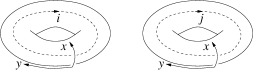
Figure 14: Gluing two solid tori $D^{2}_{xt}\times S^{1}_{y}$ without twist forms a $S^{2}\times S^{1}$. The gluing is done by identifying the $(x,y)$ point on the surface of the first torus with the $(x,-y)$ point on the surface of the second torus. If we add an additional ${\cal S}$ twist, i.e. if we identify $(x,y)$ with $(-y,-x)$, the gluing will produce a $S^{3}$.

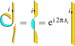
Figure 15: (Color online) A “self-loop” with canonical framing corresponds to a twist by $2\pi$. A twist by $2\pi$ induces a phase $\hskip 1.0pt\mathrm{e}^{\hskip 1.0pt\mathrm{i}\hskip 1.0pt2\pi s_{i}}$ that defines the spin $s_{i}$ of the particle.

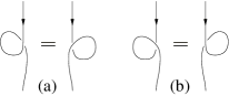
Figure 16: The two “self-loops” in (a) are “right-handed” and correspond to the same twist. The two “self-loops” in (b) are “left-handed” and also correspond to the same twist that is opposite to that in (a).

The amplitude of two linked loops, $S^{\text{Lnk}}_{ij}$, and the representation of the modular group in the excitations basis, $S$, are closely related. From Fig. 14, we see that

$$S_{ij}=\langle i|\hat{S}|j\rangle=(\text{two linked loops in }S^{3})=S^{\text{Lnk}}_{ij}Z_{\text{inv}}(S^{3}),$$ (151)

where $Z_{\text{inv}}(S^{3})$ is the volume independent part of the partition function on three-sphere $S^{3}$.Kong and Wen (2014) Since $S$ is unitary and $S^{\text{Lnk}}_{i1}=d_{i}$, we see that

$$Z_{\text{inv}}(S^{3})=1/D.$$ (152)

This way, we obtain an important relation:

$$S_{ij}=S^{\text{Lnk}}_{ij}/D,$$ (153)

that connects the amplitude of two linked loops to a modular transformation of the degenerate ground state on torus. This allows us to rewrite eqn. (146) as

$$\sum_{k}N^{ij}_{k}S_{kl}=\frac{S_{il}S_{jl}}{S_{1l}},$$ (154)

which is the Verlinde formula.

D.5 The spin $s_{i}$ of topological excitations and $T$

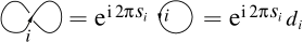
Figure 17: A figure “8” of type-$i$ string has an amplitude $\hskip 1.0pt\mathrm{e}^{2\pi\hskip 1.0pt\mathrm{i}\hskip 1.0pts_{i}}d_{i}$.

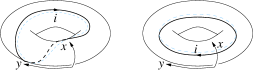
Figure 18: Gluing two solid tori $S^{1}_{x}\times D^{2}$ with an additional $\hat{T}$ twist, i.e. identifying $(x,y)$ with $(x+y,-y)$, will produce a $S^{2}\times S^{1}$. The $i$-loop in $y$-direction in the second solid torus at right can be deformed into a $i$-loop in the first solid torus at left. We see that the loop is twisted by $2\pi$ in the anti-clockwise direction.

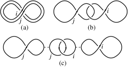
Figure 19: A double figure “8” in (a) is equal to two linked figure “8” in (b) after sliding one of the figure “8”. Applying two Y-moves to (b), we obtain (c)

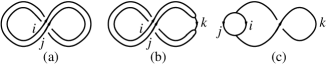
Figure 20: A double figure “8” in (a) is changed to (b) after a Y-move. (b) is equal to (c) after sliding the vertices.

We have studied two linked loops, which is a string configuration with crossing. Another important string configuration with crossing is a “self-loop” (see Fig. 15). Such a “self-loop” corresponds to a twist by $2\pi$, which equal to a straight line with a phase $\hskip 1.0pt\mathrm{e}^{\hskip 1.0pt\mathrm{i}\hskip 1.0pt2\pi s_{i}}$. Here $s_{i}$ is the spin of the type-$i$ topological excitation, which is defined mod 1. We also note that the handness of the “self-loop” determines the direction of the twist (see Fig. 16). As a result, a figure “8” of type-$i$ string has an amplitude $\hskip 1.0pt\mathrm{e}^{2\pi\hskip 1.0pt\mathrm{i}\hskip 1.0pts_{i}}d_{i}$ (see Fig. 17).

It is clear that the Dehn twist $\hat{T}$, when acting on $|i\rangle=W^{y}_{i}|1\rangle$, will twist the string $i$ by $2\pi$ and induces a phase $\hskip 1.0pt\mathrm{e}^{\hskip 1.0pt\mathrm{i}\hskip 1.0pt2\pi s_{i}}$ (see Fig. 18). The Dehn twist $\hat{T}$ also change the space-time metrics which may causes an additional $i$-independent phase, which is denoted as $\hskip 1.0pt\mathrm{e}^{-\hskip 1.0pt\mathrm{i}\hskip 1.0pt2\pi\frac{c}{24}}$. This way, we ontain another important relation:

$$T|i\rangle=\hskip 1.0pt\mathrm{e}^{-2\pi\hskip 1.0pt\mathrm{i}\hskip 1.0pt\frac{c}{24}}\hskip 1.0pt\mathrm{e}^{2\pi\hskip 1.0pt\mathrm{i}\hskip 1.0pts_{i}}|i\rangle.$$ (155)

D.6 Relation between $N^{ij}_{k}$ and $S_{ij}$

To understand the relation (34), let us compute the amplitude of a double figure “8” in two ways, as shown in Figs. 19 and 20. This allows us to show

$$\ \ \ \ Y^{\bar{j}j}_{1}Y^{\bar{i}i}_{1}DS_{i\bar{j}}\hskip 1.0pt\mathrm{e}^{2\pi\hskip 1.0pt\mathrm{i}\hskip 1.0pt(s_{i}+s_{j})}d_{i}d_{j}$$

$$=\sum_{\alpha,k}Y^{ji}_{k,\alpha}O^{ji,\alpha}_{k}\hskip 1.0pt\mathrm{e}^{2\pi\hskip 1.0pt\mathrm{i}\hskip 1.0pts_{k}}d_{k},$$ (156)

which can be simplified to (noting $\alpha=1,\cdots,N^{ij}_{k}$)

$$\frac{1}{d_{j}}\frac{1}{d_{i}}DS_{i\bar{j}}\hskip 1.0pt\mathrm{e}^{2\pi\hskip 1.0pt\mathrm{i}\hskip 1.0pt(s_{i}+s_{j})}d_{i}d_{j}=\sum_{k}N^{ij}_{k}\hskip 1.0pt\mathrm{e}^{2\pi\hskip 1.0pt\mathrm{i}\hskip 1.0pts_{k}}d_{k},$$ (157)

or

$$DS_{i\bar{j}}\hskip 1.0pt\mathrm{e}^{2\pi\hskip 1.0pt\mathrm{i}\hskip 1.0pt(s_{i}+s_{j})}=\sum_{k}N^{ij}_{k}\hskip 1.0pt\mathrm{e}^{2\pi\hskip 1.0pt\mathrm{i}\hskip 1.0pts_{k}}d_{k}.$$ (158)

Using $S_{i\bar{j}}^{*}=S_{ij}$, the above becomes eqn. (34).

In this paper, we have derived most of the $(N^{ij}_{k},s_{i},c)$ conditions, expect the condition eqn. (29). Here, we would like mention that the condition eqn. (29) can be found in LABEL:Wang10.

Appendix E List of primitive topological orders

In this section, we give lists that contain more topological orders (see Tables 11 and 12, where only the primitive topological orders are listed). The lists are generated using a different numerical code.

The abelian states with $d_{i}=1$ are described by $K$-matrices. We use the notation $(K_{11}K_{22}\cdots;K_{12}K_{23}\cdots;K_{13}K_{24}\cdots;\cdots)$ to denote the $K$-matrices.

In LABEL:SW150801111, we show that the non-abelian states can be generated by simple current algebra (SCA)Blok and Wen (1992); Wen and Wu (1994); Lu et al. (2010). (See also https://www.math.ksu.edu/$\sim$gerald/voas/ ) The SCA’s are denoted by $(R,\pm k)_{\alpha}$ (see LABEL:RSW0777,SW150801111), where $R=A_{n},B_{n},C_{n},D_{n},$ etc , and $(R,-k)_{\alpha}$ is the time-reversal conjugate of $(R,+k)_{\alpha}$. The last column of Tables 11 and 12 indicates how the corresponding topological order is realized by the $K$-matrix state or the SCA state.

References

- Landau (1937) L. D. Landau, Phys. Z. Sowjetunion 11, 26 (1937).
- Ginzburg and Landau (1950) V. L. Ginzburg and L. D. Landau, Zh. Eksp. Teor. Fiz. 20, 1064 (1950).
- Landau and Lifschitz (1958) L. D. Landau and E. M. Lifschitz, Statistical Physics - Course of Theoretical Physics Vol 5 (Pergamon, London, 1958).
- Nambu (1960) Y. Nambu, Phys. Rev. Lett. 4, 380 (1960).
- Goldstone (1961) J. Goldstone, Nuovo Cimento 19, 154 (1961).
- Tsui et al. (1982) D. C. Tsui, H. L. Stormer, and A. C. Gossard, Phys. Rev. Lett. 48, 1559 (1982).
- Bednorz and Mueller (1986) J. G. Bednorz and K. A. Mueller, Z. Phys. B 64, 189 (1986).
- Wen (2002) X.-G. Wen, Phys. Rev. Lett. 88, 11602 (2002), eprint hep-th/01090120.
- Wen (2003) X.-G. Wen, Phys. Rev. D 68, 065003 (2003), eprint hep-th/0302201.
- Levin and Wen (2006) M. Levin and X.-G. Wen, Phys. Rev. B 73, 035122 (2006), eprint hep-th/0507118.
- Wen (2013a) X.-G. Wen, Chin. Phys. Lett. 30, 111101 (2013a), eprint arXiv:1305.1045.
- You et al. (2014) Y.-Z. You, Y. BenTov, and C. Xu (2014), eprint arXiv:1402.4151.
- You and Xu (2015) Y.-Z. You and C. Xu, Phys. Rev. B 91, 125147 (2015), eprint arXiv:1412.4784.
- Anderson (1987) P. W. Anderson, Science 235, 1196 (1987).
- Baskaran et al. (1987) G. Baskaran, Z. Zou, and P. W. Anderson, Solid State Comm. 63, 973 (1987).
- Affleck and Marston (1988) I. Affleck and J. B. Marston, Phys. Rev. B 37, 3774 (1988).
- Rokhsar and Kivelson (1988) D. S. Rokhsar and S. A. Kivelson, Phys. Rev. Lett. 61, 2376 (1988).
- Affleck et al. (1988) I. Affleck, Z. Zou, T. Hsu, and P. W. Anderson, Phys. Rev. B 38, 745 (1988).
- Dagotto et al. (1988) E. Dagotto, E. Fradkin, and A. Moreo, Phys. Rev. B 38, 2926 (1988).
- Kalmeyer and Laughlin (1987) V. Kalmeyer and R. B. Laughlin, Phys. Rev. Lett. 59, 2095 (1987).
- Wen et al. (1989) X.-G. Wen, F. Wilczek, and A. Zee, Phys. Rev. B 39, 11413 (1989).
- Wen (1989) X.-G. Wen, Phys. Rev. B 40, 7387 (1989).
- Wen (1990a) X.-G. Wen, Int. J. Mod. Phys. B 4, 239 (1990a).
- Lawrence et al. (1992) T. W. Lawrence, A. Szöke, and R. B. Laughlin, Phys. Rev. Lett. 69, 1439 (1992).
- Laughlin (1983) R. B. Laughlin, Phys. Rev. Lett. 50, 1395 (1983).
- Girvin and MacDonald (1987) S. M. Girvin and A. H. MacDonald, Phys. Rev. Lett. 58, 1252 (1987).
- Zhang et al. (1989) S. C. Zhang, T. H. Hansson, and S. Kivelson, Phys. Rev. Lett. 62, 82 (1989).
- Read (1989) N. Read, Phys. Rev. Lett. 62, 86 (1989).
- Wen and Niu (1990) X.-G. Wen and Q. Niu, Phys. Rev. B 41, 9377 (1990).
- Wen (1991a) X.-G. Wen, Phys. Rev. Lett. 66, 802 (1991a).
- Wen (1990b) X.-G. Wen, Phys. Rev. B 41, 12838 (1990b).
- Wen (1992) X.-G. Wen, Int. J. Mod. Phys. B 6, 1711 (1992).
- Wen (1995) X.-G. Wen, Advances in Physics 44, 405 (1995).
- Blok and Wen (1992) B. Blok and X.-G. Wen, Nucl. Phys. B 374, 615 (1992).
- Moore and Read (1991) G. Moore and N. Read, Nucl. Phys. B 360, 362 (1991).
- Greiter et al. (1991) M. Greiter, X.-G. Wen, and F. Wilczek, Phys. Rev. Lett. 66, 3205 (1991).
- Greiter et al. (1992) M. Greiter, X.-G. Wen, and F. Wilczek, Nucl. Phys. B 374, 567 (1992).
- Wen (1993) X.-G. Wen, Phys. Rev. Lett. 70, 355 (1993).
- Wen and Zee (1992) X.-G. Wen and A. Zee, Phys. Rev. B 46, 2290 (1992).
- Wen (1999) X.-G. Wen, Phys. Rev. B 60, 8827 (1999), eprint cond-mat/9811111.
- Onnes (1911) H. K. Onnes, Comm. Phys. Lab. Univ. Leiden, Nos 119 120, 122 (1911).
- Wen (1991b) X.-G. Wen, Int. J. Mod. Phys. B 5, 1641 (1991b).
- Hansson et al. (2004) T. H. Hansson, V. Oganesyan, and S. L. Sondhi, Annals of Physics 313, 497 (2004), eprint cond-mat/0404327.
- Yoshioka et al. (1983) D. Yoshioka, B. I. Halperin, and P. A. Lee, Phys. Rev. Lett. 50, 1219 (1983).
- Haldane (1983) F. D. M. Haldane, Phys. Rev. Lett. 51, 605 (1983).
- Su (1984) W. P. Su, Phys. Rev. B 30, 1069 (1984).
- Tao and Wu (1984) R. Tao and Y.-S. Wu, Phys. Rev. B 30, 1097 (1984).
- Niu et al. (1985) Q. Niu, D. J. Thouless, and Y.-S. Wu, Phys. Rev. B 31, 3372 (1985).
- Haldane and Rezayi (1985) F. D. M. Haldane and E. H. Rezayi, Phys. Rev. B 31, 2529 (1985).
- Avron and Seiler (1985) J. E. Avron and R. Seiler, Phys. Rev. Lett. 54, 259 (1985).
- Haldane (1985) F. D. M. Haldane, Phys. Rev. Lett. 55, 2095 (1985).
- Chen et al. (2010) X. Chen, Z.-C. Gu, and X.-G. Wen, Phys. Rev. B 82, 155138 (2010), eprint arXiv:1004.3835.
- Zeng and Wen (2015) B. Zeng and X.-G. Wen, Phys. Rev. B 91, 125121 (2015), eprint arXiv:1406.5090.
- Swingle and McGreevy (2014) B. Swingle and J. McGreevy (2014), eprint arXiv:1407.8203.
- von Klitzing et al. (1980) K. von Klitzing, G. Dorda, and M. Pepper, Phys. Rev. Lett. 45, 494 (1980).
- Read and Sachdev (1991) N. Read and S. Sachdev, Phys. Rev. Lett. 66, 1773 (1991).
- Wen (1991c) X.-G. Wen, Phys. Rev. B 44, 2664 (1991c).
- Moessner and Sondhi (2001) R. Moessner and S. L. Sondhi, Phys. Rev. Lett. 86, 1881 (2001).
- Willett et al. (1987) R. Willett, J. P. Eisenstein, H. L. Strörmer, D. C. Tsui, A. C. Gossard, and J. H. English, Phys. Rev. Lett. 59, 1776 (1987).
- Radu et al. (2008) I. P. Radu, J. B. Miller, C. M. Marcus, M. A. Kastner, L. N. Pfeiffer, and K. W. West, Science 320, 899 (2008).
- Keski-Vakkuri and Wen (1993) E. Keski-Vakkuri and X.-G. Wen, Int. J. Mod. Phys. B 7, 4227 (1993).
- Wilczek and Zee (1984) F. Wilczek and A. Zee, Phys. Rev. Lett. 52, 2111 (1984).
- Kong and Wen (2014) L. Kong and X.-G. Wen (2014), eprint arXiv:1405.5858.
- Moradi and Wen (2014) H. Moradi and X.-G. Wen (2014), eprint arXiv:1401.0518.
- Wen (2012) X.-G. Wen (2012), eprint arXiv:1212.5121.
- Kane and Fisher (1997) C. L. Kane and M. P. A. Fisher, Phys. Rev. B 55, 15832 (1997), eprint cond-mat/9603118.
- Hughes et al. (2012) T. L. Hughes, R. G. Leigh, and O. Parrikar (2012), eprint arXiv:1211.6442.
- Bradlyn and Read (2015) B. Bradlyn and N. Read, Phys. Rev. B 91, 165306 (2015), eprint arXiv:1502.04126.
- Zhang et al. (2012) Y. Zhang, T. Grover, A. Turner, M. Oshikawa, and A. Vishwanath, Phys. Rev. B 85, 235151 (2012), eprint arXiv:1111.2342.
- Cincio and Vidal (2013) L. Cincio and G. Vidal, Phys. Rev. Lett. 110, 067208 (2013), eprint arXiv:1208.2623.
- Zaletel et al. (2012) M. P. Zaletel, R. S. K. Mong, and F. Pollmann (2012), eprint arXiv:1211.3733.
- Tu et al. (2013) H.-H. Tu, Y. Zhang, and X.-L. Qi, Phys. Rev. B 88, 195412 (2013), eprint arXiv:1212.6951.
- Hung and Wen (2014) L.-Y. Hung and X.-G. Wen, Phys. Rev. B 89, 075121 (2014), eprint arXiv:1311.5539.
- He et al. (2014) H. He, H. Moradi, and X.-G. Wen, Phys. Rev. B 90, 205114 (2014), eprint arXiv:1401.5557.
- Mei and Wen (2015) J.-W. Mei and X.-G. Wen, Phys. Rev. B 91, 125123 (2015), eprint arXiv:1409.5427.
- Freedman et al. (2004) M. Freedman, C. Nayak, K. Shtengel, K. Walker, and Z. Wang, Ann. Phys. (NY) 310, 428 (2004), eprint cond-mat/0307511.
- Levin and Wen (2005) M. Levin and X.-G. Wen, Phys. Rev. B 71, 045110 (2005), eprint cond-mat/0404617.
- Gu et al. (2015) Z.-C. Gu, Z. Wang, and X.-G. Wen, Phys. Rev. B 91, 125149 (2015), eprint arXiv:1010.1517.
- Kitaev and Kong (2012) A. Kitaev and L. Kong, Commun. Math. Phys. 313, 351 (2012), eprint arXiv:1104.5047.
- Gu et al. (2014) Z.-C. Gu, Z. Wang, and X.-G. Wen, Phys. Rev. B 90, 085140 (2014), eprint arXiv:1309.7032.
- Wen and Wu (1994) X.-G. Wen and Y.-S. Wu, Nucl. Phys. B 419, 455 (1994), eprint cond-mat/9310027.
- Lu et al. (2010) Y.-M. Lu, X.-G. Wen, Z. Wang, and Z. Wang, Phys. Rev. B 81, 115124 (2010), eprint arXiv:0910.3988.
- Wen and Wang (2008a) X.-G. Wen and Z. Wang, Phys. Rev. B 77, 235108 (2008a), eprint arXiv:0801.3291.
- Wen and Wang (2008b) X.-G. Wen and Z. Wang, Phys. Rev. B 78, 155109 (2008b), eprint arXiv:0803.1016.
- Barkeshli and Wen (2009) M. Barkeshli and X.-G. Wen, Phys. Rev. B 79, 195132 (2009), eprint arXiv:0807.2789.
- Seidel and Lee (2006) A. Seidel and D.-H. Lee, Phys. Rev. Lett. 97, 056804 (2006), eprint cond-mat/0604465.
- Bergholtz et al. (2006) E. J. Bergholtz, J. Kailasvuori, E. Wikberg, T. H. Hansson, and A. Karlhede, Phys. Rev. B 74, 081308 (2006), eprint cond-mat/0604251.
- Seidel and Yang (2008) A. Seidel and K. Yang (2008), eprint arXiv:0801.2402.
- Bernevig and Haldane (2008a) B. A. Bernevig and F. D. M. Haldane, Phys. Rev. Lett. 100, 246802 (2008a), eprint arXiv:0707.3637.
- Bernevig and Haldane (2008b) B. A. Bernevig and F. D. M. Haldane, Phys. Rev. B 77, 184502 (2008b), eprint arXiv:0711.3062.
- Bernevig and Haldane (2008c) B. A. Bernevig and F. D. M. Haldane (2008c), eprint arXiv:0803.2882.
- Blok and Wen (1990) B. Blok and X.-G. Wen, Phys. Rev. B 42, 8145 (1990).
- Read (1990) N. Read, Phys. Rev. Lett. 65, 1502 (1990).
- Fröhlich and Kerler (1991) J. Fröhlich and T. Kerler, Nucl. Phys. B 354, 369 (1991).
- Belov and Moore (2005) D. Belov and G. W. Moore (2005), eprint hep-th/0505235.
- Kapustin and Saulina (2011) A. Kapustin and N. Saulina, Nucl. Phys. B 845, 393 (2011), eprint arXiv:1008.0654.
- Verlinde (1988) E. Verlinde, Nuclear Physics B 300, 360 (1988).
- Andersen and Moore (1988) G. Andersen and G. Moore, Commun. Math. Phys. 117, 441 (1988).
- Vafa (1988) C. Vafa, Phys. Lett. B 206, 421 (1988).
- Etingof (2002) P. Etingof, Mathematical Research Letters 9, 651 (2002), eprint math/0207007.
-
Etingof (2009)
P. Etingof,
http://www-math.mit.edu/etingof/langsem.pdf (2009). - Witten (1989) E. Witten, Comm. Math. Phys. 121, 351 (1989).
- Gepner and Kapustin (1995) D. Gepner and A. Kapustin, Physics Letters B 349, 71 (1995), eprint hep-th/9410089.
- Rowell et al. (2009) E. Rowell, R. Stong, and Z. Wang, Comm. Math. Phys. 292, 343 (2009), eprint arXiv:0712.1377.
- Wang (2010) Z. Wang, Topological Quantum Computation (CBMS Regional Conference Series in Mathematics, 2010).
- Kitaev (2006) A. Kitaev, Annals of Physics 321, 2 (2006), eprint cond-mat/0506438.
- Schoutens and Wen (2015) K. Schoutens and X.-G. Wen (2015), eprint arXiv:1508.01111.
- Bakalov and Kirillov (2001) B. Bakalov and A. Kirillov, Lectures on Tensor Categories and Modular Functors, vol. 21 of University Lecture Series (American Mathematical Society, 2001).
- Freed and Teleman (2012) D. S. Freed and C. Teleman (2012), eprint arXiv:1212.1692.
- Freed (2014) D. S. Freed (2014), eprint arXiv:1406.7278.
- Kapustin (2014a) A. Kapustin (2014a), eprint arXiv:1403.1467.
- Kapustin (2014b) A. Kapustin (2014b), eprint arXiv:1404.6659.
- Zamolodchikov and Fateev (1985) A. Zamolodchikov and V. Fateev, Sov. Phys. JETP 62, 215 (1985).
- Gelaki et al. (2009) S. Gelaki, D. Naidu, and D. Nikshych, Algebra Number Theory 2, 959 (2009), eprint arXiv:0905.3117.
- Bruillard et al. (2014) P. Bruillard, C. Galindo, S.-H. Ng, J. Plavnik, E. C. Rowell, and Z. Wang (2014), eprint arXiv:1411.2313.
- Barkeshli and Wen (2010) M. Barkeshli and X.-G. Wen, Phys. Rev. B 81, 045323 (2010), eprint arXiv:0909.4882.
- Barkeshli and Wen (2011) M. Barkeshli and X.-G. Wen, Phys. Rev. B 84, 115121 (2011), eprint arXiv:1010.4270.
- Kitaev (2003) A. Y. Kitaev, Ann. Phys. (N.Y.) 303, 2 (2003).
- Wen (1991d) X.-G. Wen, Mod. Phys. Lett. B 5, 39 (1991d).
- Read and Rezayi (1999) N. Read and E. Rezayi, Phys.Rev. B 59, 8084 (1999), eprint cond-mat/9809384.
- Vishwanath and Senthil (2013) A. Vishwanath and T. Senthil, Phys. Rev. X 3, 011016 (2013), eprint arXiv:1209.3058.
- Wang and Senthil (2013) C. Wang and T. Senthil, Phys. Rev. B 87, 235122 (2013), eprint arXiv:1302.6234.
- Wen (2013b) X.-G. Wen, Phys. Rev. D 88, 045013 (2013b), eprint arXiv:1303.1803.
- Lan et al. (2015) T. Lan, L. Kong, and X.-G. Wen (2015), eprint arXiv:1507.04673.
- Hastings and Wen (2005) M. B. Hastings and X.-G. Wen, Phys. Rev. B 72, 045141 (2005), eprint cond-mat/0503554.
- Lan and Wen (2014) T. Lan and X.-G. Wen, Phys. Rev. B 90, 115119 (2014), eprint arXiv:1311.1784.
- Fiorenza and Valentino (2014) D. Fiorenza and A. Valentino (2014), eprint arXiv:1409.5723.
- He and Chen (2015) Y.-C. He and Y. Chen, Physical Review Letters 114, 037201 (2015), eprint arXiv:1407.2740.
- Gong et al. (2015) S.-S. Gong, W. Zhu, L. Balents, and D. N. Sheng, Phys. Rev. B 91, 075112 (2015), eprint arXiv:1412.1571.