A simple criterion for the existence of nonreal eigenvalues for a class of 2D and 3D Pauli operators
Abstract.
In this work, we investigate the discrete spectrum generated by complex matrix-valued perturbations for a class of 2D and 3D Pauli operators with nonconstant magnetic fields. We establish a simple criterion for the potentials to produce discrete spectrum near the low ground energy of the operators. Moreover, in case of creation of nonreal eigenvalues, this criterion specifies also their location.
2010 Mathematics Subject Classification. Primary: 35P20; Secondary: 81Q12, 35J10.
Keywords. Pauli operators, complex potentials, discrete spectrum, asymptotic expansions.
1. Introduction
1.1. Description of the models
We consider in this article -dimensional Pauli operators , , , defined as follows. Denote by the usual variables on and by those on . For or , let
| (1.1) |
be a magnetic field such that is an admissible magnetic field. Namely, there exists a constant satisfying
| (1.2) |
where is such that the Poisson equation admits a solution satisfying , , . By defining on and
| (1.3) |
we obtain a magnetic potential generating the magnetic field by setting
| (1.4) |
Remark 1.1.
- (i)
-
(ii)
In (1.1), stands for the intensity of the magnetic field.
-
(iii)
The case corresponds to the constant magnetic field of strength .
-
(iv)
In the three-dimensional case , the magnetic field is of constant direction and points in the -direction.
Let be a complex matrix-valued potential. Then, the Pauli operators acting on , , , are defined by
| (1.5) |
initially on , and then closed in .
For , we have the following result from [28, Propositions 1.1 and 1.2] about the spectrum of the operator :
Proposition 1.1.
Let be an admissible magnetic field with . Then, is an isolated eigenvalue of infinite multiplicity. More precisely, we have
| (1.6) |
and
| (1.7) |
where
| (1.8) |
In particular, by [29, Corollary 2.2], we have
| (1.9) |
Throughout this paper, our minimal assumptions on the potentials are the following:
Assumption (A1): For , we assume that
| (1.10) |
where for some .
Assumption (C1): For , we assume that
| (1.11) |
Examples:
-
(i)
In Assumptions (A1) and (C1), both and can be thought of the function with .
-
(ii)
In Assumption (C1), nonreal-valued potentials with , , , can be considered since obviously this implies that
1.2. State of the article
Since we will deal with non-self-adjoint operators, for convenience, we introduce some conventional definitions and notations. Let be a closed operator acting on a separable Hilbert space. An isolated point of lies in , the discrete spectrum of , if it’s algebraic multiplicity
| (1.12) |
is finite, being a small positively oriented circle centred at and containing as the only point of . Note that the geometric multiplicity of , defined by , satisfies the inequality , equality happening if is self-adjoint. We define the essential spectrum of as the set of points such that is not a Fredholm operator. Under Assumptions (A1) and (C1), we prove that is relatively compact with respect to , , . Therefore, due to the Weyl criterion on the invariance of the essential spectrum, we have , , . However, the potential may generate (complex) discrete spectrum whose only accumulation points are , see [19, Theorem 2.1, p. 373]. The distribution of the discrete spectrum near the essential spectrum for the quantum Hamiltonians has been extensively studied by various authors. However, most of the known results treat the case of self-adjoint electric potentials, see for instance [23, Chap. 11-12], [27, 39, 40, 32, 28, 3, 29, 4] and the references given there. But, recently and during the past years, there has been an increasing interest in the spectral theory of non-self-adjoint differential operators, in particular for the quantum Hamiltonians, see for instance [15, 8, 5, 11, 25, 12, 17, 22, 42, 33, 13, 9, 16]. For a detailed bibliography on the theory, we refer for instance to [42, 9]. Another results on spectral properties for non-self-adjoint operators can be found in Sjöstrand paper [38] and the references given there. Results concerning non-self-adjoint Pauli operators are much more sparse, see for instance [24], where the authors investigated the 1D Pauli equation with complex boundary conditions.
The aim of the present paper is to describe simple methods of obtaining complex eigenvalues asymptotics near the low ground energy of the 2D Pauli operator , and to show how we can construct complex matrix-valued potentials generating nonreal eigenvalues near the low ground energy of the 3D Pauli operator . Our work is closely related to [35, 34], where the author treats the case of the Schrödinger and Dirac operators with constant and nonconstant magnetic fields. Both in these papers and in the present one, the proofs of the results are inspired by previous works (on characteristic values and resonances) for self-adjoint perturbations (see [3, 4]). More precisely, here, in the 2D case, the spectral gap in allows to reduce the study of near , to that of the zeros of a holomorphic function in a punctured neighbourhood of (see Lemma 3.1 and Proposition 3.1). Hence, by this way, we can apply the general approach developed in [4] to solve our problem. On the contrary, in the 3D case, since is absolutely continuous, this reduction holds in half-disks not containing (see Lemma 6.3 and Proposition 6.2). In that case, [4]’s approach does not work and we have to use the one developed in [3] to solve our problem. The methods of this article also combine functional analysis, complex analysis, functional determinant and spectral properties of Toeplitz operators which appear when making spectral reduction near the low ground energy . The main difficulties come from the matrix-valuedness and the non-selfajointness of . Moreover, in the three-dimensional case, unlike the study of the resonances, is not supposed to be exponentially decreasing with respect to the direction of the magnetic field. Thus, the operator-valued function defined in Lemma 6.3 is not analytic near the real axis and some limiting absorption principle have to be used (see Proposition 6.2). In contrast with the Laplace operator, in [42], Wang investigated the case of in , , being a dissipative potential, where and are two measurable functions satisfying , and on an open non empty set. He proved that is not an accumulation point of the complex eigenvalues if the potential decays more rapidly than . It is still unknown, for more general complex potentials without sign restriction on the imaginary part, whether can be an accumulation point of complex eigenvalues or not. In the present work, we show that in the presence of a magnetic field, the situation is totally different. Even a compactly supported perturbation can produce clusters of eigenvalues near the low ground energy of the operators , , . More precisely, in the case , for some sufficiently small and sufficiently decreasing potential of the form
-
•
, with a positive Hermitian matrix,
-
•
, ,
we prove that is an accumulation point of a sequence of eigenvalues which are concentrated along the semi-axis (see Theorem 2.4). On the contrary, when
-
•
,
this phenomenon disappears (see Corollary 2.1). In the case , the situation is rather different in the sense we prove that is an accumulation point of a sequence of eigenvalues which are concentrated along the semi-axis , for some sufficiently decreasing potential of the form
-
•
, with a positive Hermitian matrix,
-
•
,
(see Theorem 2.2). The case of the Laplace operator is also studied in a recent preprint by Bögli [2], where nonreal potentials decaying at infinity generating infinitely many nonreal eigenvalues accumulating at each point of the essential spectrum are constructed. Upper bounds on the number of the complex eigenvalues in small annulus near the low ground energy of the operators , , , are also established here (see Theorems 2.1 and 2.3 respectively).
1.3. Organisation of the paper
The paper is organized as follows. Our main results are stated in Section 2. Section 3 is devoted to the study of the discrete spectrum near the low ground energy for the two-dimensional Pauli operator. The corresponding main results are proved in Sections 4 and 5. Section 6 is devoted to the study of the discrete spectrum near the low ground energy with respect to the three-dimensional Pauli operator, the corresponding main results being proved in Sections 7 and 8. Section 9 is a brief appendix on basic properties of Schatten-von Neumann class ideals, Section 10 a brief appendix on the theory of the index of a finite meromorphic operator-valued function, and Section 11 a brief appendix on the notion of characteristic values of operator-valued functions.
Notations
For a matrix , denotes the multiplication operator by the matrix , , , . We will denote the set of Hermitian matrices on , , . The spectral projection of onto the (infinite-dimensional) kernel of , will be denoted . Here, , , , are the components of the magnetic potential , so that is the first component of the operator . The operator will denote his second component.
2. Statement of the main results
This section is devoted to the formulation of our main results. The eigenvalues will be counted according to their algebraic multiplicity defined above. As preparation, we first recall some well-known results on Toeplitz operators. We know from [29, Lemma 2.3] that if , , then the Toeplitz operator belongs to the Schatten-von Neumann class (see Section 9 for the definition of the Schatten classes ). In particular, is a compact operator. Moreover, when it is self-adjoint and positive, the following asymptotics about the quantity , , are well-known:
- (H1)
- (H2)
-
(H3)
If has a compact support and if there exists a constant verifying on an open non-empty subset of , then by [29, Lemma 3.5],
(2.3) where .
2.1. Results for the case 2D
Let satisfy Assumption (A1). In that case, we have for any and any . Then, [29, Lemma 2.3] implies that the Toeplitz operator belongs to the Schatten-von Neumann class , . In particular, is a self-adjoint positive compact operator. For defined by (1.8), fix and introduce the punctured disk of
| (2.4) |
Our first main result gives an upper bound on the number of complex eigenvalues near the low ground energy of the operator , in small annulus.
Theorem 2.1 (Local upper bound).
Assume that Assumption (A1) holds with . Then, there exists such that for any with ,
| (2.5) |
for some constant . In particular, if is compactly supported, then satisfies the asymptotic (2.3) as .
In order to get asymptotic results, we put some restrictions on the potential .
Assumption (A2): We assume that
| (2.6) |
Denote the matrix sign of satisfying . Let and be the orthogonal projections in defined by
| (2.7) |
For , we introduce the operator
| (2.8) |
Note that is holomorphic on . Introduce the orthogonal projection onto together with the following condition:
| (2.9) |
Remark 2.1.
-
(i)
There is no loss of generality in saying is of definite sign .
-
(ii)
Actually, is compact so that condition (2.9) is generically satisfied. Namely, it is fulfilled whenever , where denotes the nonzero eigenvalue sequence of the operator .
-
(iii)
Condition (2.9) is also fulfilled for small potentials . Namely, for potentials with a real number small enough.
If , , are two positive fixed constants, and tending to zero, we define the sector
| (2.10) |
Theorem 2.2 (Localization, asymptotic behaviours).
Let satisfy Assumptions (A1) and (A2), with and of definite sign . Assume that (2.9) holds. Then, there exits such that near zero:
-
(i)
Localization: The discrete eigenvalues of with satisfy
(2.11) for any .
-
(ii)
Asymptotic: There exists a sequence of positive numbers tending to zero such that
(2.12) as .
-
(iii)
Asymptotic: If satisfies the hypotheses (H1), (H2) and (H3) above, then,
(2.13) as .
Corollaries and Remarks.
-
(i)
According to (2.1), (2.2) and (2.3), the asymptotics obtained in Theorem 2.2 essentially coincide with those obtained in [28], where the case of the self-adjoint Pauli operator with more general assumptions on is considered. Novelty in this paper is that we consider complex matrix-valued potentials .
-
(ii)
Theorem 2.2 is still true if we replace the assumption by
This condition is for instance fulfilled by potentials of the form
-
(iii)
The existence of nonreal eigenvalues and their accumulation near are ensured by assertion (ii) and (iii) of Theorem 2.2.
-
(iv)
Another way of stating assertion (i) of Theorem 2.2 is as follows: near the low ground energy of , the discrete eigenvalues of are concentrated around the semi-axis , respectively for .
-
(v)
For , we recover the standard self-adjoint electric potentials of definite sign, and (2.11) becomes . This just amounts to saying that the discrete eigenvalues are localized on the right and the left of .
- (vi)
2.2. Results for the case 3D
Let satisfy Assumption (C1) and be the multiplication operator by the function (also noted) defined by
| (2.14) |
Then, as in the case 2D, the Toeplitz operator satisfies so that it is a self-adjoint positive compact operator. In the sequel,
| (2.15) |
denotes respectively the upper and lower half-plane. For , we introduce the ring
| (2.16) |
and the half-rings
| (2.17) |
For constant, we define the domains
| (2.18) |
Our first main result gives upper bounds on the number of complex eigenvalues near the low ground energy of the operator , in small half-rings.
Theorem 2.3 (Local upper bounds).
Assume that Assumption (C1) holds with . Then, there exists such that for any with , and any ,
| (2.19) |
for some constant . In particular, if is compactly supported, then satisfies the asymptotic (2.3) as .
In what follows below, two kinds of assumption on are needed in additional.
Assumption (C2): We assume that
| (2.20) |
Remark 2.2.
-
(i)
In (2.20), when is of definite sign ( ), since the change of the sign consists to replace by , then it is sufficient to consider only .
-
(ii)
For and , the discrete eigenvalues of the operator satisfy .
With respect to Assumption (C2) above, we introduce , the multiplication operator by the function (also noted) , defined as in (2.14) with replaced by . Hence, we introduce the following exponential decay assumption:
Assumption (C3): We assume that the function satisfies
| (2.21) |
For and , we introduce the sector
| (2.22) |
where we have just excluded around the semi-axis , an angular sector of amplitude . Hence, we can formulate our second main result in this part as follows:
Theorem 2.4 (Sector free of complex eigenvalues, lower bounds).
Suppose that satisfies Assumption (C1), and Assumption (C2) with , . Then, for any small enough, there exists such that:
-
(i)
For any , the operator has no discrete eigenvalues in the sector
(2.23) -
(ii)
If furthermore satisfies Assumption (C3), then for any , there is an accumulation of nonreal eigenvalues of near zero, in a sector around the semi-axis , for
(2.24) More precisely, there exists a decreasing sequence of positive numbers , , satisfying
(2.25)
A graphic illustration of Theorem 2.4 is given in Figure 2.2.
Remark 2.3.
- (i)
- (ii)
An immediate consequence of assertion (i) of Theorem 2.4 together with (ii) of Remark 2.2 is the following:
Corollary 2.1 (Non cluster of complex eigenvalues).
Let the assumptions of Theorem 2.4 be fulfilled. Then, for any satisfying , there is no accumulation of discrete eigenvalues of near zero, for .
Actually, we expect this to be a general phenomenon in the following sense:
Conjecture 2.1.
Let satisfy Assumption (C1), with , , and of definite sign. Then, there is no accumulation of complex eigenvalues of near zero if and only if .
Remark 2.4.
To make our results in perspective, let us mention that more general situations such as: more general magnetic field in the 3D case (not supported only in the axis), and/or to consider perturbations of the magnetic field itself, are open problems.
3. Discrete eigenvalues for the 2D problem
Throughout Sections 3-5, stands for the punctured disk given by (2.4). Here and in the rest of the paper, is the constant defined by (1.8).
3.1. Preliminary results
Let and be the orthogonal projections defined by (2.7). For , on account of (1.5) with and Proposition 1.1, we clearly have
| (3.1) |
Therefore, for any lying in the resolvent set of , we have
| (3.2) |
We begin with a general result on the first term of the r.h.s. of (3.2).
Lemma 3.1.
Let with . Then, the operator-valued function
is holomorphic with values in . Furthermore,
| (3.3) |
Proof. The holomorphicity on is evident. Let us show (3.3).
The next result concerns the second term of the r.h.s. of (3.2).
Lemma 3.2.
Under the assumptions of Lemma 3.1, the operator-valued function
is holomorphic with values in . Moreover,
| (3.6) |
where is a constant depending on .
Proof. For lying in the resolvent set of , (1.5) implies that we have
| (3.7) |
Then, is well defined and analytic since is included in the resolvent set of defined on and defined on . Thus, is holomorphic on .
Now, let us prove estimate (3.6). In what follows below, constants are generic. Namely changing from a relation to another. First, let us show that (3.6) holds if is even.
Identity (3.7) implies that we have
| (3.8) |
Let us focus on the first term of the r.h.s. of (3.8). We have
| (3.9) |
By the Spectral mapping theorem, we have
| (3.10) |
Using the resolvent equation, the boundedness of the magnetic field , and applying the diamagnetic inequality (see [1, Theorem 2.3] and [37, Theorem 2.13]) which is only valid when is even, we get
| (3.11) |
By the standard criterion [37, Theorem 4.1], we have
| (3.12) |
Combining (3.9), (3.10), (3.11) and (3.12), we obtain
| (3.13) |
Arguing similarly, it can be proved that we have
| (3.14) |
Hence, for even, (3.6) holds by putting together (3.8), (3.13) and (3.14).
To prove that (3.6) holds for any , we use interpolation method. If verifies , then clearly there exists even integers satisfying and . Consider such that and introduce the operator
Denote the constant appearing in (3.6) for , , and define
By (3.6), for , . Using the Riesz-Thorin Theorem (see for instance [14, Sub. 5 of Chap. 6], [31], [41], [26, Chap. 2]), we interpolate between and to obtain the extension , with
Then, in particular, we have for any
or equivalently bound (3.6), and the lemma follows.
Now, observe that Assumption (A1) given by (1.10), implies that there exists a bounded operator such that with satisfying (1.10). Consequently, since the radius of satisfies and is bounded, then by combining identities (3.1) and (3.2) with Lemmas 3.1 and 3.2, we obtain the following:
Lemma 3.3.
The operator-valued function
is holomorphic with values in , where is defined by the polar decomposition of .
3.2. Reduction of the problem
We reduce the study of the discrete eigenvalues of near zero, to that of the zeros of a holomorphic function in a punctured neighbourhood of zero.
In what follows below, the regularized determinant is defined in Appendix A . Similarly to Lemma 3.3, it can be shown that is holomorphic in with values in . Then, is well defined by (9.2). It is well known, see for instance [37, Chap. 9], that
| (3.15) |
Since is holomorphic in , then so is the function by Property d) of Appendix A . Moreover, the algebraic multiplicity of as a discrete eigenvalue of is equal to its order as a zero of .
In the next proposition, the quantity appearing in the r.h.s. of (3.16) is defined in Appendix A .
Proposition 3.1.
Let be the operator defined in Lemma 3.3. Then, the following assertions are equivalent:
-
(i)
is a discrete eigenvalue of ,
-
(ii)
,
-
(iii)
is an eigenvalue of .
Moreover,
(3.16) where is a small contour positively oriented, containing as the unique discrete eigenvalue of .
Proof. The equivalence between assertions (i) and (ii) follows obviously from (3.15) and the equality
thanks to Property b) of Appendix A .
The equivalence between assertions (ii) and (iii) follows from Property c) of Appendix A .
We prove now (3.16). To this end, we consider the function defined by (3.15). According to the comment just after (3.15), we have
| (3.17) |
where the r.h.s. of (3.17) is the index defined by (10.2) of the holomorphic function with respect to the contour . We thus get (3.16) easily from the equality
(see for instance [4, (2.6)] for more details).
3.3. Decomposition of the weighted resolvent
Our goal in this section is to split the weighted resolvent into two parts which are respectively meromorphic and holomorphic in a neighbourhood of zero. The potential is assumed to satisfy Assumption (A1).
Proposition 3.2.
For , we have
| (3.18) |
where the operator is holomorphic in the open disk .
Remark 3.1.
4. Proof of Theorem 2.1: Upper bound
The proof will be divided into two steps.
4.1. A preliminary result
Let
| (4.1) |
denote the numerical range of the operator . The inclusion is well known (see for instance [10, Lemma 9.3.14]).
Proposition 4.1.
There exists such that for any , we have:
-
(i)
is a discrete eigenvalue of near zero if and only if is a zero of
(4.2) with a finite-rank operator analytic with respect to and satisfying
where the ’s are uniform with respect to , .
-
(ii)
Furthermore, if is a discrete eigenvalue of near zero, then,
(4.3) being chosen as in (3.16), and being the multiplicity of as a zero of .
-
(iii)
If verifies , , then is invertible and satisfies , where the is uniform with respect to , and .
Proof. (i)-(ii): By Proposition 3.2, is holomorphic near zero with values in . Then, for small enough, there exists a finite-rank operator independent of , and an operator holomorphic near zero satisfying for , and
Set and write
| (4.4) |
It is easy to check that for . Consequently, we have
| (4.5) |
where is defined by
It is a finite-rank operator of order
taking into account (3.19). Moreover, its norm is of order . Since we have for , then [19, Theorem 4.4.3] implies that
Therefore, Property (10.4) applied to (4.5) together with Proposition 3.1 give (4.3). Furthermore, it follows that is a discrete eigenvalue of near zero if and only if is a zero of .
4.2. Back to the proof of Theorem 2.1
Proposition 4.1 implies that for , we have
| (4.7) | ||||
being the eigenvalues of satisfying . Let satisfy and . Then, we have
Similarly to (4.7), it can be shown that
| (4.8) |
so that for , , we obtain
| (4.9) |
Consider the discrete eigenvalues with such that . Thanks to their discontinuous distribution, there exists a simply connected sub-domain of containing all the eigenvalues and such that . Note that in view of the definition (4.1) of the numerical range of the operator , we have
| (4.10) |
Then, Theorem 2.1 holds by applying the Jensen Lemma 11.1 with the function , , with some satisfying , , and by using (4.7) and (4.9).
5. Proof of Theorem 2.2: Localisation and asymptotics expansions
First, we have to rephrase Proposition 3.1 with respect to the characteristic value terminology (see Definition 11.1).
Proposition 5.1.
For , the following assertions are equivalent:
-
(i)
is a discrete eigenvalue of ,
-
(ii)
is a characteristic value of .
Moreover, the multiplicity of as a discrete eigenvalue coincides with its multiplicity as a characteristic value defined by (11.2).
Proof of assertion (i) of Theorem 2.2: From Proposition 5.1 and according to (ii) of Remark 3.1, we reduce the investigation of the discrete eigenvalues to that of the characteristic values of
the operator being defined by (2.8). In particular, for . Thus, assertion (i) of Theorem 2.1 holds by (i) and (ii) of Lemma 11.2 with . To be more precise, near zero, the discrete eigenvalues verify for any
| (5.1) |
the sector being defined by (2.4).
Proof of assertion (ii) of Theorem 2.2: The above proof of (i) of Theorem 2.2 together with Proposition 5.1, imply that the discrete eigenvalues near zero are the characteristic values of concentrated in the sectors , for any . In particular, we obtain
| (5.2) |
the quantity being defined by (11.3). If is the quantity defined by (11.4) with , then by using (3.19), we get
| (5.3) |
Thus, (ii) of Theorem 2.2 follows from (iii) of Lemma 11.2 together with (5.2) and (5.3).
6. Discrete eigenvalues for the 3D problem
6.1. Preliminary results
Define , , and introduce the orthogonal projections in
| (6.1) |
For , on account of (1.5) with and Proposition 1.1, we have
| (6.2) |
with the resolvent acting in . Then, for any , we have
| (6.3) |
We have the following lemma:
Lemma 6.1.
For given and , , the operator-valued function
is holomorphic with values in . Moreover,
| (6.4) |
where is a constant depending only on .
Proof. The holomorphicity on is trivial. Let us prove (6.4).
Thanks to (6.2), we have
| (6.5) |
As in (3.5), we have
| (6.6) |
From the estimate
| (6.7) |
we obtain by the Spectral mapping theorem
| (6.8) |
and by the standard criterion [37, Theorem 4.1], we obtain
| (6.9) |
Then, (6.4) follows by putting together (6.5), (6.6), (6.7), (6.8) and (6.9).
The next lemma is just the analogue of Lemma 3.2 in dimension three. It can be proved in a similar way by taking into account the appropriate modifications. For this reason, to simplify our exposition, its proof will be omitted.
Lemma 6.2.
For a given , , the operator-valued function
is holomorphic with values in . Moreover,
| (6.10) |
where is a constant depending only on .
Throughout this article, we will use the following choice of the complex square root
| (6.11) |
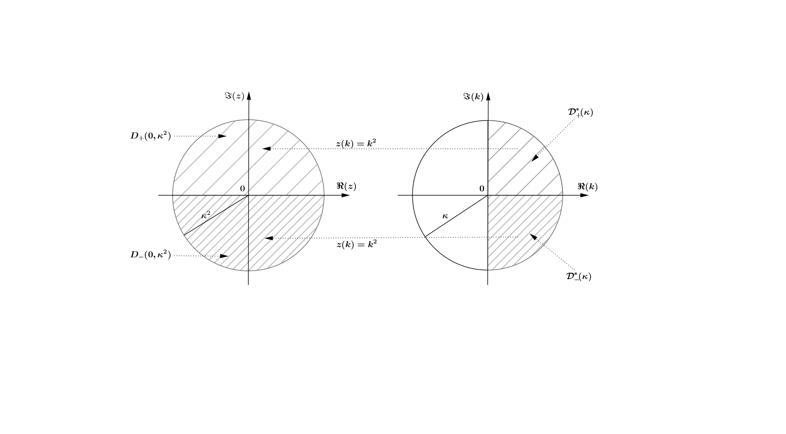
For , let be the half-rings defined by (2.17). Put the change of variables and define the domains
| (6.12) |
Under the above considerations, can be parametrized by , with respectively (see Figure 6.1 below):
Now, Assumption (C1) given by (1.11) implies that there exists a bounded operator such that , with and satisfying (1.11). Then, the boundedness of , identities (6.2), (6.3), together with Lemmas 6.1 and 6.2 give the following:
Lemma 6.3.
The operator-valued functions
are holomorphic with values in , where is defined by the polar decomposition of .
6.2. Reduction of the problem
Similarly to Lemma 6.3, we can show that is holomorphic in with values in . Then, as in (3.15), we have
| (6.13) |
We are thus led to the following proposition:
Proposition 6.1.
Let be the operator defined in Lemma 6.3. Then, the following assertions are equivalent:
-
(i)
is a discrete eigenvalue of ,
-
(ii)
,
-
(iii)
is an eigenvalue of .
Moreover,
(6.14) where is a small contour positively oriented containing as the unique point verifying is a discrete eigenvalue of .
Proof. The proof is similar to that of Proposition 3.1, taking into account the appropriate modifications.
6.3. Decomposition of the weighted resolvent
Our goal in this section is to decompose (defined just above), as a sum of a singular part at , and a holomorphic part in continuous near with values in . The potential is supposed to verify Assumption (C1).
Observe that according to the choice (6.11) of the complex square root, we respectively have for . By identity (6.3), we have
| (6.15) |
Let us focus on the first term of the r.h.s. of (6.15) and define respectively as the multiplication operators by the functions . Then, we get
| (6.16) |
For , admits the integral kernel
| (6.17) |
Then, the integral kernel of the operator is given by
| (6.18) |
With the help of (6.18), we can write
| (6.19) |
being the rank-one operator given by
| (6.20) |
and being the operator with integral kernel given by
| (6.21) |
Moreover, it is easy to observe that we have with defined by , so that is given by . Putting this together with (6.19) and (6.21), we get
| (6.22) |
where is the operator acting from to with integral kernel
| (6.23) |
Equality (6.16) combined with (6.22) give for
| (6.24) |
Finally, we get for
| (6.25) |
being defined by
| (6.26) |
More precisely, recalling that , we have with
where is the integral kernel of the orthogonal projection (see [21, Theorem 2.3]). Obviously, is given by
Therefore, it can be checked that the operator satisfies
| (6.27) |
where is the multiplication operator by the function (also noted) defined by (2.14).
For , we define as the operator with integral kernel
| (6.28) |
being defined by (6.17). Then, as in [29, (Proof of) Proposition 4.2], we can show by a limiting absorption principle that the operator-valued function is well defined and continuous. We thus have proved the following:
Proposition 6.2.
For , we have
| (6.29) |
where the operator given by
is holomorphic in and continuous on , with defined by (6.22).
Remark 6.1.
7. Proof of Theorem 2.3: Upper bounds
The proof is similar to that of Theorem 2.1.
7.1. A preliminary result
Introduce the numerical range
satisfying .
Proposition 7.1.
There exists such that for any , we have:
-
(i)
is a discrete eigenvalue of near zero if and only if is a zero of
(7.1) with a finite-rank operator analytic with respect to and satisfying
where the ’s are uniform with respect to , .
-
(ii)
Furthermore, if is a discrete eigenvalue of near zero, then we have
(7.2) being chosen as in (6.14), and being the multiplicity of as a zero of .
-
(iii)
If satisfies , , then is invertible and satisfies , where the is uniform with respect to , and .
Proof. The proof follows by arguing similarly to that of Proposition 4.1, taking into account the appropriate modifications.
7.2. Back tot the proof Theorem 2.3
Proposition 7.1 above implies that
| (7.3) | ||||
for , the being the eigenvalues of satisfying . If with , then,
Similarly to (7.3), we can show that
| (7.4) |
so that for , , we obtain
| (7.5) |
Consider the domains with and . Since the numerical range of the operator satisfies
| (7.6) |
then there exists some satisfying , . Then, Theorem 2.3 follows by applying the Jensen Lemma 11.1 with the function , , together with (7.3) and (7.5).
8. Proof of Theorem 2.4: Sectors free of complex eigenvalues and lower bounds
To simplify, we give the proof only for the case . The case follows in a similar way by replacing by .
(i): For any small enough, set and introduce the sector
| (8.1) |
According to (ii) of Remark 6.1, for any , we have
| (8.2) |
being a self-adjoint positive operator independent of , while is holomorphic in and continuous on . Since we have
then it is easy to see that the operator is invertible for . Otherwise, it can be shown that we have
| (8.3) |
Therefore, for , it can be checked that
| (8.4) |
. Then, we have
| (8.5) |
where
| (8.6) |
Since is continuous on , then there exists a uniform constant such that . Putting this together with (8.4) and (8.6), it follows immediately that is invertible for , , and
| (8.7) |
This means that is not a discrete eigenvalue.
(ii): Let denote the sequence of the decreasing nonzero eigenvalues of taking into account their multiplicity. If Assumption (C3) given by (2.21) is fulfilled, then similarly to [3, (Proof of) Lemma 7], it can be shown that there exists a positive constant such that
| (8.8) |
Since the nonzero eigenvalues of and coincide, then there exists a decreasing sequence of positive numbers , , such that
| (8.9) |
Moreover, there exists for any a path , where
| (8.10) |
(see Figure 8.1), enclosing the eigenvalues of lying in .
Obviously, the operator is invertible for , and it can be proved that
| (8.11) |
where
| (8.12) |
Introduce the path . According to the construction of and (8.11), we immediately observe that is invertible for with
| (8.13) |
Then, for , we have
| (8.14) |
By choosing sufficiently small and using Property e) of Subsection 9 given by (9.3), we obtain
| (8.15) |
for any . More precisely, if we let , be the constants defined by (8.7), the one defined by (8.12), and that defined by (9.3), then (8.15) holds whenever satisfies
| (8.16) |
where
| (8.17) |
Thus, the Rouché Theorem implies that the number of zeros of enclosed in taking into account their multiplicity, is equal to that of enclosed in taking into account their multiplicity. This number is equal to . Hence, thanks to Proposition 6.1 and Property (10.4) applied to (8.14), bound (2.25) follows immediately since the zeros of are the discrete eigenvalues of taking into account their multiplicity. From the fact that the sequence is infinite tending to zero, it follows the infiniteness of the number of the discrete eigenvalues claimed. This concludes the proof of Theorem 2.4.
9. Appendix A : Schatten-von Neumann ideals and regularized determinants
For the convenience of the reader, we repeat the relevant material from Reed-Simon [30], Simon [36, 37], and Gohberg-Goldberg-Krupnik [20], thus making our exposition self-contained.
Let be a separable Hilbert space and be the set of compact linear operators on . Denote by the -th singular value of . The Schatten-von Neumann classes are defined by
| (9.1) |
To simplify, we will write when no confusion can arise. For and , the regularized determinant is defined by
| (9.2) |
Here are some elementary properties about this determinant (see for instance [36]):
a) .
b) For , the class of bounded linear operators on , if and belong to , then .
c) is invertible if and only if .
d) If is a holomorphic operator-valued function in a domain , then so is in .
e) is Lipschitz as function on uniformly on balls. Explicitly, we have
| (9.3) |
by [36, Theorem 6.5], for some constant .
10. Appendix A : Index of a finite meromorphic operator-valued function
The space and the class are defined as in Appendix A 1. We have the following definition from [19, Definition 4.1.1].
Definition 10.1.
Let be a neighbourhood of a fixed point , and be a holomorphic operator-valued function. The function is said to be finite meromorphic at if its Laurent expansion at has the form
| (10.1) |
where for , the operators are of finite rank. Moreover, if is a Fredholm operator, then the function is said to be Fredholm at . In that case, the Fredholm index of is called the Fredholm index of at .
If a function is holomorphic in a neighbourhood of a contour (positively oriented), its index with respect to this contour is defined by
| (10.2) |
Let us point out that if is holomorphic in a domain with , then thanks to the residues theorem, coincides with the number of zeros of in taking into account their multiplicity.
In what follows below, denotes the class of invertible linear operators on the Hilbert space . Let be a connected domain, be a pure point and closed subset, and be a finite meromorphic operator-valued function which is Fredholm at each point of . The index of with respect to the contour is defined by
| (10.3) |
where the operator does not vanish in the integration contour . The following properties are well known:
| (10.4) |
for a trace class operator-valued function, we have
| (10.5) |
We refer for instance to [19, Chap. 4] for a deeper discussion on the subject.
11. Appendix A : Jensen type inequality and characteristic values of operator-valued functions
The following lemma (see for instance [3, Lemma 6] for a proof) contains a version of the well-known Jensen inequality.
Lemma 11.1.
Let be a simply connected sub-domain of and let be holomorphic in with continuous extension to . Assume that there exists such that and for (the boundary of ). Let be the zeros of repeated according to their multiplicity. For any domain , there exists such that , the number of zeros of contained in , satisfies
| (11.1) |
Consider a domain of containing , and let be a holomorphic operator-valued function, being as above.
Definition 11.1.
For a domain , a complex number is a characteristic value of , if is not invertible. The multiplicity of a characteristic value is defined by
| (11.2) |
where is a small contour positively oriented containing as the unique point satisfying is not invertible.
Define
Once there exists satisfying is not invertible, then by the analytic Fredholm theorem, the set is pure point. Hence, we set
| (11.3) |
In the sequel, we suppose that the operator is self-adjoint and we put
| (11.4) |
the number of eigenvalues of lying in the interval , taking into account their multiplicity. The orthogonal projection onto is denoted .
Lemma 11.2.
[4, Corollary 3.4, Corollary 3.9, Corollary 3.11] Let be as above with invertible. Let be a bounded domain such that is smooth and transverse to the real axis at each point of .
-
(i)
If , then for sufficiently small, . So, the characteristic values satisfy near .
-
(ii)
Moreover, if satisfy , then the characteristic values satisfy respectively near .
-
(iii)
For fixed, let be defined as in (2.10). Assume that there exists a constant such that
with growing unboundedly as . Then, there exists a positive sequence which tends to such that
(11.5) -
(iv)
If we have
with for any small enough, then
(11.6)
References
- [1] J. Avron, I. Herbst, B. Simon, Schrödinger operators with magnetic fields. I. General interactions, Duke Math. J. 45 (1978), 847-883.
- [2] S. Bögli, Schrödinger operators with non-zero accumulation points of complex eigenvalues, arxiv 1605.09356.
- [3] J.-F. Bony, V. Bruneau, G. Raikov, Resonances and Spectral Shift Function near the Landau levels, Ann. Inst. Fourier, 57(2) (2007), 629-671.
- [4] J.-F. Bony, V. Bruneau, G. Raikov, Counting function of characteristic values and magnetic resonances, Commun. PDE. 39 (2014), 274-305.
- [5] A. Borichev, L. Golinskii, S. Kupin, A Blaschke-type condition and its application to complex Jacobi matrices, Bull. London Math. Soc. 41 (2009), 117-123.
- [6] Behrndt, An Open Problem: Accumulation of Nonreal Eigenvalues of Indefinite Sturm–Liouville Operators, Int. Eq. Op. Theory, 77 (2013) 299-301.
- [7] V. Bruneau, A. Pushnitski, G. Raikov, Spectral shift function in strong magnetic fields, Algebra in Analiz, 16 (2004), 207-238; St. Petersburg Math. J. 16 (2005), 181-209.
- [8] V. Bruneau, E. M. Ouhabaz, Lieb-Thirring estimates for non-seladjoint Schrödinger operators, J. Math. Phys. 49 (2008).
- [9] J.-C Cuenin, A. Laptev, C. Tretter, Eigenvalues estimates for non-selfadjoint Dirac operators on the real line, Ann. Hen. Poincaré 15 (2015), 707-736, ISSN: 1424-0637.
- [10] E. B. Davies, Linear Operators and their Spectra, Camb. Stu. Adv. Math. 106 (2007), Cambridge University Press.
- [11] M. Demuth, M. Hansmann, G. Katriel, On the discrete spectrum of non-seladjoint operators, J. Funct. Anal. 257(9) (2009), 2742-2759.
- [12] M. Demuth, M. Hansmann, G. Katriel, Eingenvalues of non-selfadjoint operators: a comparison of two approaches, Operator Theory: Advances and Applications, 232, 107-163.
- [13] C. Dubuisson, On quantitative bounds on eigenvalues of a complex perturbation of a Dirac operator, Int. Eq. Operator Theory 78(2) (2014), 249–269.
- [14] G. B. Folland, Real analysis Modern techniques and their applications, Pure and Apllied Mathematics, (1984), John Whiley and Sons.
- [15] R. L. Frank, A. Laptev, E. H. Lieb, R. Seiringer, Lieb-Thirring inequalities for Schrödinger operators with complex-valued potentials, Lett. in Math. Phys. 77 (2006), 309-316.
- [16] R. L. Frank, A. Laptev, O. Safronov, On the number of eigenvalues of Schrödinger operators with complex potentials, J. London Math. Soc., (2016) doi: 10.1112/jlms/jdw039, arXiv:1601.03122.
- [17] L. Golinskii, S. Kupin, On discrete spectrum of complex perturbations of finite band Schrödinger operators, in "Recent trends in Analysis", Proceedings of the conference in honor of N. Nikolsi, Université Bordeaux 1, 2011, Theta Foundation, Bucharest, Romania, 2013.
- [18] I. Gohberg, E. I. Sigal, An operator generalization of the logarithmic residue theorem and Rouché’s theorem, Mat. Sb. (N.S.) 84 (126) (1971), 607-629.
- [19] I. Gohberg, J. Leiterer, Holomorphic operator functions of one variable and applications, Operator Theory, Advances and Applications, vol. 192 Birkhäuser Verlag, 2009, Methods from complex analysis in several variables.
- [20] I. Gohberg, S. Goldberg, N. Krupnik, Traces and Determinants of Linear Operators, Operator Theory, Advances and Applications, vol. 116 Birkhäuser Verlag, 2000.
- [21] B. C. Hall, Holomorphic methods in analysis and mathematical physics, In: First Summer School in Analysis and Mathematical Physics, Cuernavaca Morelos, 1998, 1-59, Contemp. Math. 260, AMS, Providence, RI, (2000).
- [22] M. Hansmann, Variation of discrete spectra for non-selfadjoint perturbations of selfadjoint operators, Int. Eq. Op. Theory, 76(2) (2013) 163-178.
- [23] V. Ya. Ivrii, Microlocal Analysis and Precise Spectral Asymptotics, Springer-Verlag, Berlin, 1998.
- [24] D. Kochan, D. Krejcirik, R. Novák, P. Siegl, The Pauli equation with complex boundary conditions, J. Phys. A: Math. Theory, 45 (2012) 444019.
- [25] A. Laptev, O. Safronov, Eigenvalue estimates for Schrödinger operators with complex potentials, Comm. Math. Phys. 292(1), (2009), 29–54.
- [26] A. Lunardi, Interpolation Theory, Appunti Lecture Notes, 9 2009, Edizioni Della Normale.
- [27] M. Melgaard, G. Rozenblum Eigenvalue asymptotics for weakly perturbed Dirac and Schröinger operators with constant magnetic fields of full rank, Commun. PDE. 28 (2003), 697-736.
- [28] G. D. Raikov, Spectral asymptotics for the perturbed 2D Pauli Operator with oscillating magnetic Fields. I. Non-zero mean value of the magnetic field, Markov Process. Related Fields 9 (2003), 775-794.
- [29] G. D. Raikov, Low energy asymptotics of the spectral shift function for Pauli operators with nonconstant magnetic fields Publ. Res. Inst. Math. Sci. 46 (2010), 565–590.
- [30] M. Reed, B. Simon, Scattering Theory III, Methods of Modern Mathematical Physics, (1979), Academic Press, INC.
- [31] M. Riesz, Sur les maxima des formes bilinéaires et sur les fonctionnelles linéaires, Acta Math. 49 (1926), 465-497.
- [32] G. Rozenblum, S. Solomyak, Counting Schrödinger boundstates: semiclassics and beyond, Sobolev spaces in mathematics. II, 329–353, Int. Math. Ser. (N. Y.), 9, Springer, New York, 2009.
- [33] D. Sambou, Lieb-Thirring type inequalities for non-self-adjoint perturbations of magnetic Schrödinger operators, J. Funct. Anal. 266 (8), (2014), 5016-5044.
- [34] D. Sambou, A criterion for the existence of nonreal eigenvalues for a Dirac operator, New York J. Math. 22 (2016) 469-500.
- [35] D. Sambou, On eigenvalue accumulation for non-self-adjoint magnetic operators, to appear in Journal de Mathématiques Pures et Appliquées, preprint on ArXiv: 1506.06723.
- [36] B. Simon, Notes on infinite determinants of Hilbert space operators, Adv. in Math. 24 (1977), 244-273.
- [37] B. Simon, Trace ideals and their applications, Lond. Math. Soc. Lect. Not. Series, 35 (1979), Cambridge University Press.
- [38] J. Sjöstrand, Spectral properties of non-self-adjoint operators, preprint on http://arxiv.org/abs/1002.4844
- [39] A. V. Sobolev, Asymptotic behavior of the energy levels of a quantum particle in a homogeneous magnetic field, perturbed by a decreasing electric field. I, J. Sov. Math. 35 (1986), 2201-2212.
- [40] H. Tamura, Asymptotic distribution of eigenvalues for Schrödinger operators with homogeneous magnetic fields, Osaka J. Math, 25 (1988), 633-647.
- [41] G. O. Thorin, An extension of a convexity theorem due to M. Riesz, Kungl. Fysiografiska Saellskapet i Lund Forhaendlinger 8 (1939), no. 14.
- [42] X. P. Wang, Number of eigenvalues for a class of non-selfadjoint Schrödinger operators, J. Math. Pures Appl. 96(9) (2011), no. 5, 409-422.