Flocking with discrete symmetry: the 2d Active Ising Model

Abstract

We study in detail the active Ising model, a stochastic lattice gas where collective motion emerges from the spontaneous breaking of a discrete symmetry. On a 2d lattice, active particles undergo a diffusion biased in one of two possible directions (left and right) and align ferromagnetically their direction of motion, hence yielding a minimal flocking model with discrete rotational symmetry. We show that the transition to collective motion amounts in this model to a bona fide liquid-gas phase transition in the canonical ensemble. The phase diagram in the density/velocity parameter plane has a critical point at zero velocity which belongs to the Ising universality class. In the density/temperature ‘canonical’ ensemble, the usual critical point of the equilibrium liquid-gas transition is sent to infinite density because the different symmetries between liquid and gas phases preclude a supercritical region. We build a continuum theory which reproduces qualitatively the behavior of the microscopic model. In particular we predict analytically the shapes of the phase diagrams in the vicinity of the critical points, the binodal and spinodal densities at coexistence, and the speeds and shapes of the phase-separated profiles.

I Introduction

Active matter systems, defined as large assemblies of interacting particles consuming energy to self-propel, exhibit a variety of elaborate collective behaviors. Among them, collective motion—a term referring to the coherent displacement of large groups of individuals over length scales much larger than their individual size—has played a leading role in active matter studies. It can be observed in a wide range of biological systems such as bird flocks Ballerini2008 , fish schools fish ; fishHugues , bacterial swarms Steager2008 ; PeruaniMB , actin Schaller2010 or microtubule SuminoNature2010 motility assays, but also in inert matter that is artificially self-propelled, for example in assemblies of vibrated polar disks Deseigne2010 , rolling colloids BartoloNature or self-propelled liquid droplets Thutupalli .

On the theoretical side, the transition to collective motion—hereafter referred to as the “flocking” transition—has attracted the attention of the physics community because simple models have proved useful to describe its generic properties, highlighting the possibility of universal behaviours. The model introduced by Vicsek and collaborators two decades ago Vicsek1995 is prototypical of this line of research, containing only two ingredients: self-propulsion at a constant speed and aligning interactions. It has often been described as a dynamical XY model TT since the alignment of the particle directions of motion resemble the ferromagnetic alignment of XY spins.

The phenomenology of the Vicsek model is now well established Vicsek1995 ; Gregoire2004 ; SolonVMPRL2015 . When decreasing the noise on the aligning interaction, or increasing the density, a transition takes place from a disordered gas into an ordered state of collective motion. Between these two homogeneous phases lays a region of parameter space where particles gather in dense ordered bands travelling in a dilute disordered background. These bands, which are a robust feature of flocking models Gregoire2004 ; Mishra2010 ; Weber2013 ; PeruaniGliders ; Farrell2012 ; BDG ; Ihle , are a signature of the first-order nature of the transition, together with intermittency, metastability and hysteresis Gregoire2004 ; SolonVMPRL2015 . Unfortunately, they are seen only in large systems and strong finite size effects render the numerical study of the Vicsek model (VM) very costly in computing power.

To overcome these numerical difficulties and gain more insight into the flocking transition, a number of analytical approaches have been followed. Hydrodynamic equations for Vicsek-like models have been either derived by coarse-graining BDG ; Ihle or proposed phenomenologically TT ; Ramaswamy2005 ; Mishra2010 . These equations predict phase diagrams in qualitative agreement with the microscopic models, including the existence of inhomogeneous bands BDG ; Ihle ; Mishra2010 ; SolonVMPRL2015 . Their analytical study is however so complicated that little can be done beyond working with their linearized version. Nevertheless, some progress was made to account for the long range order and giant density fluctuations observed in the ordered phase of the Vicsek model TT . Interestingly, it was also recently shown that all hydrodynamic equations derived for polar flocking models BDG ; Mishra2010 ; Ihle ; Solon2013 admit the same family of 1d propagative solutions Caussin . A complete analytical study of the Vicsek model, from micro to macro, however remains elusive.

An alternative strategy to gain insight into the flocking transition relied on the introduction of an Active Ising Model (AIM) Solon2013 which circumvents both the numerical and analytical pitfalls of the Vicsek model. Using non-equilibrium versions of ferromagnetic models has indeed often proven a useful strategy DDS ; PeruaniGliders ; KimPRE2015 ; Eaves . The AIM, which we study in detail in this paper, contains the two key ingredients for flocking: self-propulsion and aligning interactions. The continuous rotational symmetry of the Vicsek model is however replaced by a discrete symmetry; In the AIM, particles diffuse in the 2d plane but are self-propelled in only one of two possible directions (left or right). It is thus akin to a dynamical Ising model where particles have a discrete rotational symmetry. The AIM is found to have a simpler, more tractable, behavior than the Vicsek-like models with continuous symmetry while still retaining a large part of their physics. Using a lattice-based model also simplifies both numerical and analytical studies.

After introducing the model in section II, we present a numerical study of the 2d AIM in section III. Our main conclusion is that the transition in the AIM amounts to a liquid-gas transition in the canonical ensemble. At fixed orientational noise, the system can be in two “pure” states: a disordered gas or an ordered liquid, the latter leading to a collective migration of all particles to the left or to the right. When constraining the system’s density to lie between two ’spinodal lines’, no homogeneous phase can be observed and the system phase-separates, with an ordered travelling liquid band coexisting with a disordered gas background. A key difference with the usual equilibrium liquid-gas transition is that liquid and gas have different symmetries; A supercritical region is thus prohibited since one has to break a symmetry to take the system from a gas to a liquid state, which explains the atypical shape of the phase diagram.

In section IV, we complement our numerical approach by deriving a set of hydrodynamic equations for the dynamics of the local density and magnetisation fields. Interestingly, a simple mean-field theory wrongly predicts a continuous transition, failing to account for the phase-separated profiles. A refined mean-field model, taking into account the fluctuations of the density and magnetisation fields, reproduces qualitatively the phenomenology of the AIM. In section V, we use the hydrodynamic equations to compute at large densities the shape of the phase-separated profiles, the coexisting densities, the velocity of the liquid domain and account for the finite-size scalings observed in the microscopic model. Finally, we argue in section VI in favor of the robustness of our results by considering an off-lattice version of the model and different boundary conditions.

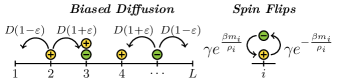
Figure 1: Sketch of the two possible actions and their rates of occurrence. The ferromagnetic interaction between particles is purely on-site and particles diffuse freely. Beyond the biased diffusion shown here, particles also hop symmetrically up or down, with equal rates $D$ in both directions.

II Definition of the model

We consider $N$ particles moving on a 2D lattice of $L_{x}\times L_{y}$ sites with periodic boundary conditions. Each particle carries a spin $\pm 1$ and there are no excluded volume interactions between the particles: there can thus be an arbitrary number $n_{i}^{\pm}$ of particles with spins $\pm 1$ on each site $i\equiv(i_{1},i_{2})$. The local densities and magnetizations are then defined as $\rho_{i}=n^{+}_{i}+n^{-}_{i}$ and $m_{i}=n^{+}_{i}-n_{i}^{-}$. We consider a continuous-time Markov process in which particles can both flip their spins and hop to neighboring lattice sites at rates that depend on their spins (see Fig. 1). The hopping and flipping rates, detailed in the next subsections, are such that our model is endowed with self-propulsion and inter-particle alignment, hence consituting a flocking model with discrete symmetry.

II.1 Alignment: Fully connected Ising models

A particle with spin $s$ on site $i$ flips its spin at rate

$$W(s\to-s)=\gamma\exp\left(-s\beta\frac{m_{i}}{\rho_{i}}\right),$$ (1)

where $\beta=1/T$ plays the role of an inverse temperature. These rates satisfy detailed balance with respect to an equilibrium distribution $P\propto\exp[-\beta H]$ where $H$ is the sum over the $L_{x}L_{y}$ lattice sites of the Hamiltonians of fully connected Ising models:

$$H=-\sum_{\text{sites }i}\frac{1}{2\rho_{i}}\sum_{j=1}^{\rho_{i}}\sum_{k\neq j}S^{i}_{j}S^{i}_{k}=-\sum_{\text{sites }i}\left[\frac{m_{i}^{2}}{2\rho_{i}}-\frac{1}{2}\right]$$ (2)

The first sum runs over the lattice site index $i=(i_{1},i_{2})$, the next two over the particles $j,k$ present on site $i$, and $S^{i}_{j}=\pm 1$ is the value of spin $j$. (The factor $1/2$ simply avoids double counting.) The rate $\gamma$ can always be absorbed in a change of time unit so that we take $\gamma=1$, silently omitting it from now on.

This interaction is purely local: particles only align with other particles on the same site and, without particle hopping, the model amounts to $L^{2}$ independent fully connected Ising models. The factor $1/\rho_{i}$ in $W$ makes the Hamiltonian $H$ extensive with $N$ and keeps the interaction rates bounded: the rate $W(s\to-s)$ at which a particle of spin $s$ flips its spin varies between $\exp(-\beta)$ if all the other particles on the same site have spins $s$ to $\exp[\beta(1-2/\rho_{i})]$ if they all have spins $-s$.

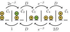
Figure 2: A loop of four configurations involving 2 particles on 2 sites breaking Kolmogorov’s criterionKolmo showing that the system does not satisfy detailed balance even when $\varepsilon=0$. The numbers associated to the arrows are the transition rates for $\varepsilon=0$. The product of the transition rates along $\mathcal{C}_{1}\to\mathcal{C}_{2}\to\mathcal{C}_{3}\to\mathcal{C}_{4}\to\mathcal{C}_{1}$ (left to right) is $2D^{2}e^{-2\beta}$, whereas the reverse order (right to left) yields $2D^{2}e^{-\beta}$.

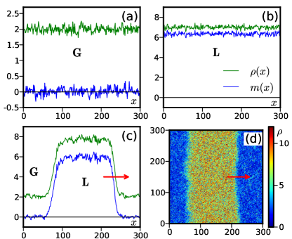
Figure 3: (a-c) Examples of density profiles (green upper line) and magnetization profiles (blue lower line) averaged along vertical direction for the three phases. (a) Disordered gas, $\beta=1.4$, $\rho_{0}=2$. (b) Polar liquid, $\beta=2$, $\rho_{0}=7$. (c) Liquid-gas coexistence, $\beta=1.6$, $\rho_{0}=5$. (d) 2d snapshot corresponding to (c). (for all figures $D=1$, $\varepsilon=0.9$)

II.2 Self-propulsion: Biased diffusion

Particles also undergo free diffusion on the lattice, with a left/right bias depending on the sign of their spins: a particle with spin $s$ hops with rate $D(1+s\varepsilon)$ to its right, $D(1-s\varepsilon)$ to its left, and $D$ in both the up and down directions. There is thus a mean drift, which plays the role of self-propulsion, with particles of spins $\pm 1$ moving along the horizontal axis with an average velocity $\pm 2D\varepsilon$.

The model is designed to have the self-propulsion entering in a minimal and tunable way through the parameter $\varepsilon$. Importantly, the limit of vanishing self-propulsion $\varepsilon\to 0$ is well-defined because the spins still diffuse on the lattice. This dynamics should thus allow us to interpole continuously between ‘totally self-propelled’ ($\varepsilon=1$), self-propelled ($\varepsilon\in]0,1[$), weakly self-propelled ($\varepsilon\sim 1/L$) and purely diffusive $(\varepsilon=0)$ particles.

This differs from the Vicsek model where the zero-velocity limit corresponds to immobile particles undergoing an equilibrium dynamics resembling that of the XY model, with a quenched disorder on the bonds (only particles closer than a fixed distance interact).

Let us note, however, that even when $\varepsilon=0$ the model is not at equilibrium i.e. it does not satisfy detailed balance with respect to any distribution. This is easily shown using Kolmogorov’s criterion Kolmo . In Fig. 2, we exhibit a loop of four configurations such that the products of the transition rates for visiting the loop in one order, $\mathcal{C}_{1}\to\mathcal{C}_{2}\to\mathcal{C}_{3}\to\mathcal{C}_{4}\to\mathcal{C}_{1}$, and the reverse order are different, whence a violation of detailed balance. To make the $\varepsilon=0$ limit an equilibrium dynamics, one strategy could be to choose hopping rates satisfying detailed balance with respect to the Hamiltonian H defined in (2), replacing $D$ by $D\exp(-\beta\Delta H/2)$). The steady-state distribution would however be factorized and not very interesting. An alternative would be to further add to (2) nearest neighbours interactions but we have not followed this cumbersome path here. Actually, as we show in section III.2, this microscopic irreversibility when $\varepsilon=0$ is irrelevant at large scales and we recover in this limit a phase transition belonging to the Ising universality class.

II.3 Simulations

To simulate the dynamics of the model, we used a random-sequential-update algorithm. We discretized the time in small time-steps $\Delta t$. A particle is then chosen at random; it flips its spin $s$ with probability $W(s\to-s)\Delta t$, hops upwards or downwards with probabilities $D\Delta t$, to its right or to its left neighboring sites with probabilities $D(1\pm s\varepsilon)\Delta t$. Finally, it does nothing with probability $1-[4D+W(s\to-s)]\Delta t$. Time is then incremented by $\Delta t/N$ and we iterate up to some final time. In practice we used $\Delta t=[4D+\exp(\beta)]^{-1}$ to minimize the probability that nothing happens while keeping all probabilities smaller than one.

Note that this algorithm does not allow a particle to be updated twice (on average) during $\Delta t$ and is thus an approximation of our continuous-time Markov process. We also used continuous-time simulations, associating clocks to each particle or each site and pulling updating times from the corresponding exponential laws. In practice we did not find any difference in the simulation results but the continuous time simulations were often slower so that we mostly used the random sequential update algorithm.

In most of this article we use simulation boxes with $L_{x}\times L_{y}$ lattice sites and periodic boundary conditions. In section VI.1 we discuss what happens for closed boundary conditions.

Figure 4: Phase-separated density (left) and magnetization (right) profiles as the density increases. Parameters: $\beta=2$, $D=1$, $\varepsilon=0.9$, system of size 800x100. The profiles have been averaged over time and along the $y$ axis.

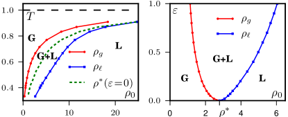
Figure 5: Phase diagrams of the AIM. The red and blue lines delimit the region of existence of phase-separated profiles. Left: Parameter spaces ($T=1/\beta$, $\rho_{0}$) for $D=1$. Red and blue coexistence lines correspond to $\varepsilon=0.9$ while the green dashed line indicates the critical points at $\varepsilon=0$. Right: Parameter space ($\varepsilon$, $\rho_{0}$) for $D=1$, $\beta=1.9$. At $\varepsilon=0$ we recover critical point in the Ising universality class.

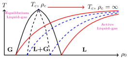
Figure 6: Schematic picture of the differences between the phase diagrams of the passive and active liquid gas transition. In the active case, because the liquid and the gas have different symmetries, the critical point is sent to $\rho=\infty$, thus suppressing the supercritical region.

III A Liquid-Gas Phase Transition

We explored the phase diagram using three control parameters: the temperature $T=\beta^{-1}$, the average density $\rho_{0}=N/(L_{x}L_{y})$, and the self-propulsion ‘speed’ $\varepsilon$. Doing so, we observed three different phases shown in Fig. 3. For $\varepsilon\neq 0$, at high temperatures and low densities, the particles fail to organize and we observe a homogeneous gas of particles with local magnetization $\langle m_{i}\rangle\approx 0$. On the contrary, for large densities and small temperatures, the particles move collectively either to the right or to the left, forming a polar liquid state with $\langle m_{i}\rangle=m_{0}\neq 0$. For intermediate densities, when $\rho_{0}\in[\rho_{g}(T,\epsilon),\,\rho_{\ell}(T,\epsilon)]$, the system phase separates into a band of polar liquid traveling to the left or to the right through a disordered gaseous background.

The lines $\rho_{g}(T,\epsilon)$ and $\rho_{\ell}(T,\epsilon)$ both delimit the domain of existence of the phase-separated profiles and play the role of coexistence lines: As shown in Fig. 4, for all phase-separated profiles at fixed $T,\,\epsilon$, the densities in the gas and liquid part of the profiles are $\rho_{g}$ and $\rho_{\ell}$, respectively. Correspondingly, the magnetization are $0$ and $m_{\ell}(T,\epsilon)\neq 0$. Thus, varying the density $\rho_{0}$ at constant temperature and propulsion speed solely changes the width of the liquid band. Consequently, in the phase coexistence region, the lever rule can be used to determine the liquid fraction $\Phi$ in the same way as for an equilibrium liquid-gas phase transition in the canonical ensemble:

$$\Phi=\frac{\rho_{0}-\rho_{g}}{\rho_{\ell}-\rho_{g}}$$ (3)

As we shall see below, this analogy goes beyond the sole shape of the phase-separated profiles and the phase-transition to collective motion of the active Ising model is best described as a liquid-gas phase transition rather than an order-disorder one.

III.1 Temperature-density ‘canonical’ ensemble

The phase diagram in the ($T$, $\rho_{0}$) parameter plane, computed for $\varepsilon=0.9$, is shown in the left panel of Fig. 5. While the general structure of the phase diagram, with a gas phase, a liquid phase, and a coexistence region, is reminiscent of an equilibrium liquid-gas phase diagram, the shapes of the transition lines are unusual. This difference can be understood using a symmetry argument. Since the disordered gas and the polar liquid have different symmetries, the system cannot continuously transform from one homogeneous phase to the other without crossing a transition line. There is thus no super-critical region and the critical point is sent to $T_{c}=1$ and $\rho_{c}=\infty$. (See Fig. 6 for a schematic picture.)

This symmetry argument should be rather general for flocking transitions separating a disordered state and a symmetry-broken state of collective motion. Indeed, in Vicsek-like models, where the role of the inverse temperature is played by the noise intensity, the phase diagrams are qualitatively similar to the one shown in Fig. 5. This is true both for the full phase diagram recently computed in SolonVMPRL2015 as well as for earlier results Gregoire2004 , for a slightly different kinetic model and its hydrodynamic theory BDG , but also for an active nematic Vicsek-like model Sandrine and a hydrodynamic theory of self-propelled rods Peshkov2012 .

III.2 Velocity-density ensemble

Conversely, one can change the strength of the self-propulsion $\varepsilon$ while keeping the temperature fixed. Again, one obtains a phase diagram with three regions. The difference with the canonical ensemble is that in this parameter plane, the two coexistence lines merge at $\varepsilon=0$, where self-propulsion vanishes, yielding a critical point at a finite density $\rho^{*}(T)$ (See the right panel of Fig. 5). The curve $\rho^{*}(T)$ is reported in the left panel of Fig. 5 and satisfies $\rho^{*}(T)\in[\rho_{g}(T,\varepsilon),\rho_{\ell}(T,\varepsilon)]$. In section III.6 we show that this critical point belongs to the Ising universality class.

The shape of this phase diagram is identical to the one computed in Mishra2010 for a phenomenological hydrodynamic description of self-propelled particles with polar alignment. The comparison with other microscopic models in the literature is however hard to make since there seems to be very few studies in the $(\varepsilon,\rho_{0})$ plane, probably because very few models admit a well-defined zero velocity limit.

III.3 Nucleation vs spinodal decomposition

As for an equilibrium liquid-gas transition, the coexistence lines $\rho_{g}(T,\varepsilon)$ and $\rho_{\ell}(T,\varepsilon)$ are complemented by spinodal lines $\varphi_{g}(T,\varepsilon)$ and $\varphi_{\ell}(T,\varepsilon)$ that mark the limit of linear stability of the homogeneous gas and liquid phases, respectively. While $\rho_{g}$ and $\rho_{\ell}$ are easily measured in simulations, $\varphi_{g}$ and $\varphi_{\ell}$ are much harder to access numerically at non-zero temperature: When the system is in the coexistence region but outside the putative spinodal lines, the homogeneous phases are metastable and finite fluctuations make the system phase-separate. The closer to the spinodal line, the faster this nucleation occurs and it is then difficult to pinpoint precisely the transition from a ‘fast’ nucleation to a spinodal decomposition. Nevertheless, the differences between the coexistence and spinodal regions are clearly seen when, starting from a homogeneous phase, one quenches the system in the coexistence region but relatively far away from the spinodal lines.

Quenching outside the spinodal region, the homogeneous phases are metastable. The closer to the binodals, the longer it takes for a liquid (resp. gas) domain to be nucleated in the gas (resp. liquid) background. The convergence to the phase-separated steady-state then results from the coarsening of this domain.

Figure 7: Successive snapshots following quenches from homogeneous gas and liquid phases inside and outside the spinodal region. Parameters: $D=1,\varepsilon=0.9,\beta=1.8$, system sizes 400x400 and 1000x1000 for the quenches from the gas and liquid phases. From top to bottom, $\rho_{0}=1.84,\,3,\,3,\,4.7$. See Supplementary Movies in SI .

Quenching inside the spinodal region, the different symmetries between gas and liquid result in different spinodal decomposition dynamics when starting from ordered and disordered phases. Starting from a disordered gas, the linear instability almost immediately results in the formation of an extensive number of small clusters of negative and positive spins. The coarsening then stems from the merging of these clusters, until a single, macroscopic domain remains. The late stage of the coarsening is thus dominated by the long-lived competition between a small number of right- and left-moving macroscopic clusters. Their shapes (see Fig. 8) are reminiscent of the counter-propagating arrays of bands reported in FreyPRX , where it was suggested, using deterministic simulations of the Boltzmann equation derived for kinetic flocking models, that such profiles could constitute a new phase of flocking models. In our simulations, we always observed a coarsening process leading to a single band, which seems to indicate that the apparent stability of these solutions in FreyPRX could be due to the lack of fluctuation terms. It would nevertheless be interesting to make a more detailed study of the coarsening dynamics to see if these alternating bands could indeed form a stable phase (for instance at low temperatures, where the coarsening seems to become slower and slower).

Figure 8: Snashots in the late stage of coarsening taken from the same simulation as the first row of fig. 7 at time $t=283000$ (left) and $t=310000$ (right). Parameters: $D=1,\varepsilon=0.9,\beta=1.8,\rho_{0}=3$, system sizes 400x400.

Starting from the ordered phase, the linear instability results in many liquid domains which all move in the same direction. The coarsening then results from the collision of liquid bands that move in the same direction, but with slightly different speeds. See Fig. 7 and SI movies SI for examples of these four possible dynamics.

III.4 Hysteresis loops

Another similarity with a liquid-gas transition is the presence of hysteresis loops obtained by varying slowly the density at constant $\beta$ and $\varepsilon$ in finite-size systems. Such loops are shown in the left panel of Fig. 9, where the liquid fraction $\Phi$ is reported as the density is continuously ramped up and down. To measure $\Phi$ numerically, a first strategy, followed in Solon2013 , is to compute average density profiles at fixed $\rho_{0}$, as shown in the left panel of Fig. 4 and use an arbitrary density treshold between $\rho_{g}$ and $\rho_{\ell}$ to associate each site to the gas or liquid regions.

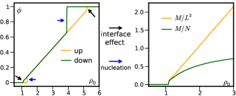
Figure 9: Left: Evolution of the liquid fraction $\phi$ upon changing continuously $\rho_{0}$. Large jumps in $\Phi$ correspond to the nucleation of bands in meta-stable homogeneous profiles while small jumps are finite-size effects due to the finite width of the interfaces connecting the gas and liquid regions. The density is increased by $\delta\rho_{0}=0.02$ every $\Delta t=2000$. $L_{x}\times L_{y}=800\times 100,\,\beta=2,\,\varepsilon=0.9,\,D=1$. Right Evolution of the magnetisations per particles and per sites as the density is varied. The linear scaling typical of liquid-gas phase transition is seen using $m_{L}=M/L^{2}$.

Since the interfaces between gas and liquids are not perfectly straight, this is slightly artefactual for finite-size systems. Here we decided to measure $\Phi$ numerically through:

$$\Phi_{\rm num.}=\frac{1}{m_{\ell}L_{x}L_{y}}\sum_{i}m_{i}$$ (4)

where $m_{\ell}$ is the magnetization of the plateau in the liquid part of the profile. ($m_{\ell}$ is independent of $\rho_{0}$ as long as the system is phase-separated and corresponds to the magnetization of a uniform liquid phase at the coexistence density $\rho_{\ell}$.) The results are very similar to those obtained in Solon2013 but first (4) is faster to measure and second it does not rely on an arbitrary density treshold.

Starting in the gas phase and increasing the density, the system remains disordered, with a liquid fraction $\phi=0$, until a band of liquid is nucleated, at which point $\phi$ jumps to a finite value. Increasing again $\rho_{0}$, the liquid region widens until the two interfaces between gas and liquid almost touch and the liquid phase almost fills the system. At that point, the system jumps to a homogeneous liquid phase with $\phi=1$.

Upon decreasing the density, a similar scenario occurs: A homogeneous liquid becomes metastable as the coexistence line is crossed. As the density keeps decreasing, the system thus remains in a liquid state with $\Phi=1$ until a nucleation event brings it to a phase-separated profile. The liquid region then shrinks until its boundaries almost touch and a second discontinuity of $\Phi$ occurs as the system jumps into a homogeneous gas phase.

III.5 Order parameter and finite-size scaling

The liquid-gas transition picture suggests different finite-size scaling and order parameter than those associated to magnetic phase transitions previously used to study flocking models. Most studies Vicsek1997 ; Martin1999 ; Gregoire2004 indeed relied on the mean magnetization per particle

$$m_{N}=\frac{1}{N}\sum_{i}m_{i}$$ (5)

rather than the mean magnetization per unit area

$$m_{L}=\frac{1}{L_{x}L_{y}}\sum_{i}m_{i}=\rho_{0}m_{N}$$ (6)

For models like the Vicsek model, the former is nothing but the polarisation ${\bf m}_{N}={\bf P}$ while the latter is related to the total momentum ${\bf m}_{L}=\rho_{0}{\bf P}/v$. In the phase-separated region, both can be related to the liquid fraction $\Phi$ through Eq. (3)

$$m_{N} =\frac{1}{N}\Phi L_{x}L_{y}m_{\ell}=m_{\ell}\frac{1-\rho_{g}/\rho_{0}}{\rho_{\ell}-\rho_{g}}$$ (7)

$$m_{L} =\Phi m_{\ell}=m_{\ell}\frac{\rho_{0}-\rho_{g}}{\rho_{\ell}-\rho_{g}}$$ (8)

The simple linear scaling of $m_{L}$ with $\rho_{0}-\rho_{g}$ is replaced by a non-linear dependence of $m_{N}$ with $\rho_{0}$, as shown in Fig. 9, right panel. An apparently inoccent change of the normalization used to make the magnetisation $M=\sum_{i}m_{i}$ intensive can thus turn the simple affine scaling of $m_{L}$ with $\rho_{0}$, typical of a liquid-gas transition, into the non-linear dependence of $m_{N}$ that could make one mistake the transition for a critical one.

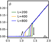
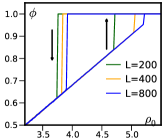
Figure 10: Hysteresis loops for system sizes 200x100, 400x100 and 800x100. For each system, the density is increased by $\delta\rho_{0}=0.02$ every $\Delta t=2000$. $T=0.5$, $\varepsilon=0.9$.

Let us now go back to the hysteresis loops and discuss their finite size scaling. As shown in figure 10, the discontinuities of the liquid fraction get closer and closer to the binodals $\rho_{g}$ and $\rho_{\ell}$ as the system size increases, leading to vanishingly small hysteresis loops in the thermodynamic limit.

Consider first the transition from gas to phase-separated profiles. The liquid fraction exhibits two different discontinuities when the density is decreased or increased, due to two different effects. As the density is decreased, phase-separated profiles cannot be maintained arbitrarily close to $\rho_{g}$. There is indeed a critical nucleus, which roughly amounts to two connected domain walls, as can be seen in Fig. 4 for $\rho_{0}=1.2$. As shown on Fig. 11 (left), this critical nucleus $L_{c}$ is independant of the system size. If the excess mass $L_{x}L_{y}(\rho_{0}-\rho_{g})$ is smaller than a critical value $\varphi_{c}L_{y}$, this critical nucleus cannot be accomodated in the system, which thus falls into the gas phase. As the system size increases, the minimal density to observe phase-separated profiles $\rho_{0}=\rho_{g}+\varphi_{c}/(L_{x})$ thus converges to $\rho_{g}$ as $L_{x}$ increases and phase-separated profiles are seen closer and closer to the binodal. The second discontinuity, met upon increasing the density, corresponds to the nucleation of a liquid band of width $L_{b}$ in a gaseous background. Since $L_{b}$ can be anything between $L_{c}$ and $L_{x}$, increasing the system size at fixed density should decrease the mean time until nucleation of such bands, thanks to an entropic contribution due to the number of places where the bands can be nucleated. As shown in 10, this is indeed the case and the transition to phase-separated profiles thus also happens closer and closer to the binodal $\rho_{g}$.

The same line of reasoning can be used to understand the scaling of the second hysteresis window, close to $\rho_{\ell}$. Thus, in the thermodynamic limit, all discontinuities disappear and the liquid fraction varies continuously from $\phi=0$ at $\rho_{0}=\rho_{g}$ to $\phi=1$ at $\rho_{0}=\rho_{\ell}$, as for an equilibrium liquid-gas transition in the canonical ensemble. Note that the width of the critical nucleus diverges as one gets closer and closer to the critical points ($\varepsilon=0$ or $\beta=1$), as shown in the right panel of Fig. 11. This could explain why some studies of the Vicsek model in the small velocity region claim to find a critical transition AlbanoVM : as one gets closer and closer to the zero speed limit, the system-size above which one can correctly observe the discontinuous nature of the transition diverges.

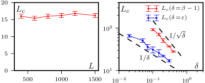
Figure 11: Left: Divergence of the critical nucleus $L_{c}$ when approaching the critical points $\beta\to 1$ and $\varepsilon\to 0$. To measure $L_{c}$, we started in the phase-separated state and decreased continuously the density (the errorbars correspond to the density step used) to record the density $\rho_{m}$ at which the liquid band disappears. $L_{c}$ is then defined by $L\rho_{m}=L\rho_{g}+L_{c}(\rho_{\ell}-\rho_{g})$, as the length of a band at density $\rho_{\ell}$ that can be made with the excess density $\rho_{m}-\rho_{g}$. Right: Variation of the critical nucleus iwht $L$ showing that, within numerical errors, it does not depend on system size. Parameters: $D=1$, $\varepsilon=0.9$, $\beta=1.9$

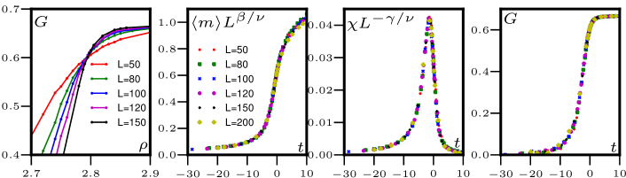
Figure 12: Left: Binder cumulant $G(\rho)$ from which we find the critical density $\rho^{*}=2.798\pm 0.002$. Other three figures: data collapse on the universal scaling functions $F_{m}$, $F_{\chi}$ and $F_{G}$ (defined in the text) when the data is rescaled with the 2d Ising exponent values $\beta=1/8$, $\gamma=7/4$ and $\nu=1$. $t=L^{1/\nu}(\rho-\rho^{*})/\rho^{*}$. Parameters: $D=1$, $\varepsilon=0.9$, $\beta=1.9$.

III.6 The $\epsilon=0$ critical point

While the $\beta=1$, $\rho_{c}=\infty$, critical point is out of reach numerically, the study of the $\varepsilon=0$ critical point is accessible. At $\varepsilon=0$, there is no self-propulsion and the phase transition is of a completely different nature from the liquid-gas transition described above. As we show below, despite the dynamics being non-equilibrium, it turns out to be a standard critical phase transition belonging to the Ising universality class.

We studied this critical point using a finite-size scaling standard for magnetic systems at criticality Binder1997 . We thus consider the magnetization $m_{N}\in[0,1]$. In equilibrium, around ferromagnetic critical points, the order parameter, susceptibility and Binder cumulant $G=1-\frac{\langle m^{4}\rangle}{\langle m^{2}\rangle^{2}}$ are known Binder1997 to obey the finite-size scaling relations

$$\langle m\rangle=L^{-\beta/\nu}F_{m}(tL^{1/\nu})$$ (9)

$$\chi=L^{2}(\langle m^{2}\rangle-\langle m\rangle^{2})=L^{\gamma/\nu}F_{\chi}(tL^{1/\nu})$$ (10)

$$G=F_{G}(tL^{1/\nu})$$ (11)

where $t=L^{1/\nu}(\rho-\rho^{*})/\rho^{*}$ is the rescaled distance to the critical density $\rho^{*}$. $F_{m}$, $F_{\chi}$ and $F_{G}$ are universal scaling functions and $\beta$, $\gamma$ and $\nu$ the usual critical exponents.

We used the fact that $G(t=0)$ is independent of $L$ to find the critical density, which is thus the density where all the curves $G(t)$ for different system sizes intersect (Fig. 12, left). We found that the value at the crossing point is the same universal value $G(t=0)\simeq 0.61$ as in the 2d Ising model Kamieniarz . A very neat data collapse is further observed for the critical exponents of the 2d Ising model $\beta=1/8$, $\gamma=7/4$ and $\nu=1$ (see Fig. 12). We thus conclude that the critical point at $\varepsilon=0$ is indeed in the Ising universality class.

Note that a direct evalutation of the critical exponents is much harder than for the equilibrium Ising model. Here, the dynamics is fixed so one cannot use alternative dynamics like cluster algorithms to circumvent the problem of critical slowing down.

III.7 Number fluctuations

In most flocking models the homogeneous ordered phase exhibits giant density fluctuations Gregoire2004 ; huguesMetric ; Mishra2010 ; Dey2012 ; Sandrine . These are quantified by measuring number fluctuations, i.e by counting the number of particles $n(\ell)$ in boxes of increasing sizes $\ell<L$ and computing its root mean square $\Delta n(\ell)$. When the correlation length ${\cal L}$ is finite, a box of size $\ell\gg{\cal L}$ can be divided in $(\ell/{\cal L})^{2}$ independant boxes. The total number of particles in the large box is then the sum of independent identically distributed random variables; The central limit theorem applies and the probability distribution of $n(\ell)$ tends to a Gaussian. This yields the “normal” scaling $\Delta n\sim n^{1/2}$. On the contrary, one finds in the Vicsek model the anomalous scaling $\Delta n\sim n^{0.8}$ Gregoire2004 .

In the Active Ising model the number fluctuations are found to be normal in the liquid and gas phases, where $\Delta n\sim n^{1/2}$, and trivially ‘giant’ in the phase-separated regime where $\Delta n\sim n$ (see Fig. 13).

Note that the scaling $\Delta n\sim n$ is a simple consequence of phase-separation and one should thus distinguish this scaling from the ‘anomalous’ scaling of the Vicsek model, which is a signature of long-range correlations. Let us consider a system at liquid fraction $\phi$ that is large enough that we can find a range of box sizes $\ell$ such that: 1) $\ell\ll L$ so that we can neglect the contribution of the interfaces (a box is either in the liquid or the gas phase); 2) $\ell$ is large enough that $n(\ell)$ takes only two possible values and we can neglect the fluctuations around these two values. With these assumptions,

$$P(n)\simeq\phi\delta(n-\rho_{\ell}\ell^{2})+(1-\phi)\delta(n-\rho_{g}\ell^{2})$$ (12)

where $\rho_{\ell}$ and $\rho_{g}$ are the densities in the gas and liquid domains. Then one finds

$$\langle n\rangle =(\phi\rho_{\ell}+(1-\phi)\rho_{g})\ell^{2}=\rho_{0}\ell^{2}$$ (13)

$$\Delta n =\sqrt{\langle n^{2}\rangle-\langle n\rangle^{2}}=\sqrt{\phi(1-\phi)}\frac{\rho_{\ell}-\rho_{g}}{\rho_{0}}\langle n\rangle$$ (14)

which is a simple hand-waving explanation of the scaling observed in the coexistence region of the active Ising model, as well as in other phase-separating systems Aranson2008 ; Fily2012 .

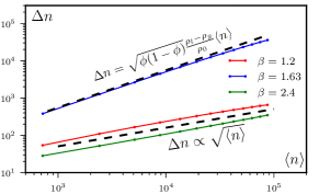
Figure 13: Number fluctuations in the three different phases: gas (red), liquid (green) and at coexistence (blue, upper line). $n$ is the number of particles in boxes of size $\ell$ and $\Delta n$ its root mean square. $D=1$, $\varepsilon=0.9$, $L=400$, $\rho_{0}=5$

IV Hydrodynamic description of the Active Ising Model

In this section we derive and analyze a continuous description of the AIM based on two coupled partial differential equations accounting for the spatio-temporal evolutions of the density and magnetization fields.

We first show in section IV.1 that a standard mean-field treatment wrongly predicts a continuous transition between the disordered gas and the ordered liquid. In section IV.2 we show that local fluctuations, which are neglected in the mean-field approximations, are necessary to correctly account for the physics of the system when the density is finite and $\varepsilon\neq 0$. We show in particular that as soon as the density is finite, fluctuations make the transition first order. We then use our hydrodynamic description in section V to study the inhomogeneous profiles.

IV.1 Mean-field equations

The simplest way to account analytically for a non-equilibrium lattice gas is probably to derive mean-field equations. These are known to be quantitatively wrong, but they often capture phase diagrams correctly Blythe2007 ; Sugden .

Their derivations follow a standard procedure which can be applied to the AIM and which, for simplicity, we first present in 1D. Starting from the master equation, one first derives the time-evolution of the mean number of $\pm 1$ spins on site $i$

$$\langle\dot{n}_{i}^{\pm}\rangle =D(1\pm\varepsilon)\langle n_{i-1}^{\pm}\rangle+D(1\mp\varepsilon)\langle n_{i+1}^{\pm}\rangle-2D\langle n_{i}^{\pm}\rangle$$

$$\pm\langle n_{i}^{-}\exp(\beta\frac{m_{i}}{\rho_{i}})\rangle\mp\langle n_{i}^{+}\exp(-\beta\frac{m_{i}}{\rho_{i}})\rangle$$ (15)

which can then be rewritten for the density and magnetisation

$$\langle\dot{\rho}_{i}\rangle =D(\langle\rho_{i+1}\rangle+\langle\rho_{i-1}\rangle-2\langle\rho_{i}\rangle)-D\varepsilon(\langle m_{i+1}\rangle-\langle m_{i-1}\rangle)$$ (16)

$$\langle\dot{m}_{i}\rangle =D(\langle m_{i+1}\rangle+\langle m_{i-1}\rangle-2\langle m_{i}\rangle)-D\varepsilon(\langle\rho_{i+1}\rangle-\langle\rho_{i-1}\rangle)$$

$$+2\langle\rho_{i}\sinh(\beta\frac{m_{i}}{\rho_{i}})\rangle-2\langle m_{i}\cosh(\beta\frac{m_{i}}{\rho_{i}})\rangle$$ (17)

One can then take a continuum limit using the rescaled variable $\tilde{x}=i/L\in[0,1]$, $\tilde{D}=D/L^{2}$, $\tilde{v}=2D\varepsilon/L$ and use the Taylor expansion $\rho_{i\pm 1}\equiv\rho(x)\pm L^{-1}\partial_{x}\rho(x)+L^{-2}\partial_{xx}\rho(x)/2$. We then obtain equations for the continuum fields $\rho(x)$, $m(x)$, which are assumed to smoothly interpolate the discrete occupancies $\rho_{i}$, $m_{i}$:

$$\partial_{t}\langle\rho\rangle =\tilde{D}\partial_{\tilde{x}\tilde{x}}\langle\rho\rangle-\tilde{v}\partial_{\tilde{x}}\langle m\rangle$$ (18)

$$\partial_{t}\langle m\rangle =\tilde{D}\partial_{\tilde{x}\tilde{x}}\langle m\rangle-\tilde{v}\partial_{\tilde{x}}\langle\rho\rangle+\left\langle 2\rho\sinh\frac{\beta m}{\rho}-2m\cosh\frac{\beta m}{\rho}\right\rangle$$ (19)

In higher dimension, the sole difference is that the diffusive terms become $\tilde{D}\Delta\langle\rho\rangle$ and $\tilde{D}\Delta\langle m\rangle$ whereas the $\tilde{v}$ terms still involve solely $\partial_{\tilde{x}}$ since the hopping is biased only horizontally.

In practice, to compare microscopic simulations and hydrodynamic theories it is often easier not to rescale space and use a continuous variable $x=L\tilde{x}\in[0,L]$ (and hence $D=\tilde{D}L^{2}$ and $v=L\tilde{v}=2D\varepsilon$). Macroscopic and microscopic transport parameters are then expressed in the same units and equations (18) and (19) are then valid, without the tilde variables. This is what we use in the following.

Equations (18) and (19) are exact; they couple the first moments $\langle\rho\rangle$ and $\langle m\rangle$ to higher moments through the averages of the hyperbolic sine and cosine functions. Following the standard procedure established for equilibrium ferromagnetic models, we then make two approximations. First, we take a mean-field approximation by replacing $\langle f(\rho,m)\rangle$ by $f(\langle\rho\rangle,\langle m\rangle)$, for any function $f$. (We then drop the $\langle\dots\rangle$ notation for clarity.) This amounts to neglecting both the correlations between density and magnetisation and their fluctuations. Second, we expand the hyperbolic functions in power series, up to $m^{2}/\rho^{2}$. This further restricts our description to the case where $m\ll\rho$. We then arrive at the mean-field equations

$$\dot{\rho} =D\Delta\rho-v\partial_{x}m$$ (20)

$$\dot{m} =D\Delta m-v\partial_{x}\rho+2m(\beta-1)-\alpha\frac{m^{3}}{\rho^{2}}$$ (21)

where $\alpha=\beta^{2}(1-\beta/3)$. (For $\beta>3$, one should expand to higher order to obtain a stabilizing term.)

Let us consider the various terms appearing in the mean-field equations. The first terms on the r.h.s of (20) and (21) are diffusion terms arising from the stochastic particle hopping. Let us stress that these terms do not depend on the bias $\varepsilon$ and are thus present even in the totally asymmetric case $\varepsilon=1$; they do not rely on the possibility for $+1$ and $-1$ particles to hop backwards and forwards, respectively. The second terms, proportional to $v$, are due to the bias. Their physical origin is explained in Fig. 14 where we show how positive gradients in $m$ or $\rho$ yield negative contributions to $\dot{\rho}$ or $\dot{m}$, respectively. Finally, the last two terms in (21) stem from the ferromagnetic interaction and, apart from the $\rho^{2}$ dependence of the last term, are typical of $\phi^{4}$ Landau mean-field theory. Note that the alignment terms are the only non-linear ones and thus the only terms for which the mean-field approximation is actually an approximation.

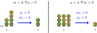
Figure 14: Schematic account for the role of density and magnetisation gradients in the mean-field equations. Left: Initially, $m=0$ and $\nabla\rho>0$ around site $i$. Once plus particles jump to the right and minus particles to the left, the density in site $i$ is unchanged but $m_{i}$ has decreased. Right: Initially, $\rho$ is constant and $\nabla m<0$ around site $i$. Once particles have jumped, the magnetisation of site $i$ is unchanged but the density has decreased.

The mean-field equations always accept the trivial homogeneous solution

$$\rho(x)=\rho_{0},\qquad m(x)=0\,,$$ (22)

which is linearly stable for $\beta<1$. As soon as $\beta>1$, two ordered homogeneous solutions appear,

$$\rho=\rho_{0},\qquad m=\pm\rho_{0}\sqrt{\frac{2(\beta-1)}{\alpha}}\,,$$ (23)

which are linearly stable (see the left panel of Fig. 15). Therefore, at the mean-field level, a linearly stable homogeneous solution exists for all ($\beta$, $\rho_{0}$). Furthermore, integrating numerically Eqs. (20) and (21) starting from different initial conditions foot1 , the system always relaxes to a homogeneous solution and inhomogeneous profiles are never observed. Hence, the mean-field equations predict a continuous transition between homogeneous disordered and ordered profiles at $\beta=1$, just as for the Weiss ferromagnet Weiss . The phase diagram is simply split between a high-temperature disordered homogeneous phase, for $T>1$, and a low temperature ordered homogeneous phase, for $T<1$. This mean-field approach thus completely misses the phenomenology of the microscopic model; It cannot explain the existence of phase-separated profiles and yield a phase diagram corresponding to a single (continuous) transition line at $T=1$, in contradiction to the crescent shape observed in the microscopic model (see Fig. 5).

IV.2 Going beyond the mean-field approximation

Previous coarse-graining approaches of flocking models BDG ; Baskaran2008 ; Farrell2012 ; Tsimring often relied on neglecting correlations by factorizing probability distributions. For example, in the Boltzmann-Ginzburg-Landau approach of Bertin et al. BDG the two-particle probability distribution is replaced by the product of one-particle distributions. In our case, to derive the mean-field equations (20) and (21) we made an even cruder approximation.

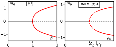
Figure 15: Linear stability of homogeneous profiles in the naive (left) and refined (right) mean-field models. Plain (resp. dashed) lines denote stable (resp. unstable) solutions. In the RMFM, for $\beta<1$, only the homogeneous profile exists and is stable at all densities.

When computing, for instance, the first non-linear term $\langle m^{3}/\rho^{2}\rangle$, neglecting correlations between $m$ and $\rho$ leads to

$$\langle m^{3}/\rho^{2}\rangle=\langle m^{3}\rangle\left\langle\frac{1}{\rho^{2}}\right\rangle$$ (24)

We went one step further, completely discarding fluctuations and replaced $\langle 1/\rho^{2}\rangle$, $\langle m^{3}\rangle$ by $1/\langle\rho\rangle^{2}$, $\langle m\rangle^{3}$. As we show below, these fluctuations are crucial to account qualitatively for the physics of the AIM.

The dynamical equations (18) and (19) on the first moments predict how $\langle\rho(x,t)\rangle$ and $\langle m(x,t)\rangle$ evolve in time, given an initial distribution

$${\cal P}[\rho,m]=\delta(\rho(x)-\rho_{0})\delta(m(x)-m_{0}).$$ (25)

The mean-field approximation then amounts to compute the averages of hyperbolic functions in (19) by assuming that, as time goes on, ${\cal P}$ remains a product of Dirac functions:

$${\cal P}[\rho,m;x,t\,|\,\rho_{0},m_{0}] =\delta(\rho(x,t)-\bar{\rho}(x,t))$$ (26)

$$\quad\times\delta(m(x,t)-\bar{m}(x,t))$$

where $\bar{\rho}(x,t)$ and $\bar{m}(x,t)$ are solutions of the mean-field equations (20) and (21). In practice this means that repeatedly simulating the microscopic model starting from an initial distribution (25) always yields the exact same values $\rho(x,t)=\bar{\rho}(x,t)$ and $m(x,t)=\bar{m}(x,t)$. A better description should allow both $\rho$ and $m$ to fluctuate around their mean values as well as account for their correlations.

We can thus improve our approximation by replacing the dirac functions in (26) by Gaussians of variance $\sigma_{\rho}^{2}(x,t)$ and $\sigma_{m}^{2}(x,t)$. This still neglects correlations between $\rho$ and $m$ but allows for (small) fluctuations around their mean. Note that the only approximation made in the derivation of the mean-field equations occured at the level of the alignment terms. Since each site of the AIM is a fully connected Ising model, it is reasonnable to assume that in the large density limit, mean-field should be correct. We thus assume that our corrections to mean-field should be small in the high density regions, where it is also reasonnable to assume that the variance of $\rho(x,t)$ and $m(x,t)$ are proportional to $\bar{\rho}$: $\sigma_{\rho}^{2}=\alpha_{\rho}\bar{\rho}$ and $\sigma_{m}^{2}=\alpha_{m}\bar{\rho}$ where $\alpha_{\rho}$ and $\alpha_{m}$ are functions of $\beta$ and $v$ only.

The probability to observe given values of $\rho(x,t)$ and $m(x,t)$ is then assumed to be

$${\cal P}[\rho,m;x,t\,|\,\rho_{0},m_{0}]={\cal N}(\rho-\bar{\rho},\alpha_{\rho}\bar{\rho}){\cal N}(m-\bar{m},\alpha_{m}\bar{\rho})$$ (27)

where ${\cal N}(x,\sigma^{2})=e^{-x^{2}/\sigma^{2}}/\sqrt{2\pi\sigma^{2}}$ is the normal distribution.

Under these assumptions, the alignment term in (19) can still be computed analytically; We show in appendix A that, at leading order in a $\bar{m}/\bar{\rho}$ expansion, the correction to mean-field reads

$$\left\langle 2\rho\sinh\frac{\beta m}{\rho}-2m\cosh\frac{\beta m}{\rho}\right\rangle\approx 2(\beta-1-\frac{r}{\bar{\rho}})\bar{m}-\alpha\frac{\bar{m}^{3}}{\bar{\rho}^{2}}$$ (28)

where $r=3\alpha\alpha_{m}/2$ is a positive function of $\beta$. Intuitively, the fluctuations “renormalize” the transition temperature

$$\beta_{t}(\rho)=1+\frac{r}{\rho}=\beta_{t}^{MF}+\frac{r}{\rho}$$ (29)

In principle, one could expand $\beta_{t}$ to higher order to obtain a better and better approximation. The correction (29) however suffices to account qualitatively for the most salient features of the microscopic model and we will thus stop our expansion at this order. Furthermore, extending (28) to higher orders does not suffice to provide quantitative agreement between microscopic simulations of the AIM and the “corrected” mean-field equations, probably because we still neglect correlations between $\rho$ and $m$. More details are provided in appendix A for the interested reader.

IV.3 Refined Mean-Field Model

The correction to mean-field derived in the previous section can thus be seen as a finite-density correction to the transition temperature $\beta_{t}$, which converges to its mean-field value $\beta_{t}^{MF}=1$ as $\rho\to\infty$. As was already recognized in previous studies BDG ; Baskaran2008 ; Mishra2010 ; Peshkov2012 , the density-dependence of $\beta_{t}$ is the key ingredient to describe phase separation at the level of hydrodynamic equations. With this correction, we obtain a refined mean-field model (RMFM)

$$\dot{\rho} =D\Delta\rho-v\partial_{x}m$$ (30)

$$\dot{m} =D\Delta m-v\partial_{x}\rho+2(\beta-1-\frac{r}{\rho})m-\alpha\frac{m^{3}}{\rho^{2}}$$ (31)

which we now study.

The linear stability analysis of homogeneous solutions strongly differs from the mean-field case. For $\beta>1$ the disordered profile is stable for $\rho_{0}\in[0,\varphi_{g}(\beta)]$ where

$$\varphi_{g}(\beta)=r/(\beta-1)$$ (32)

The homogeneous ordered solutions

$$\rho(x)=\rho_{0},\quad m(x)=m_{0}\equiv\pm\rho_{0}\sqrt{2\frac{\beta-1}{\alpha}-2\frac{r}{\rho_{0}\alpha}}$$ (33)

exist for all $\rho_{0}>\varphi_{g}$, but are only stable for $\rho_{0}\geq\varphi_{\ell}>\varphi_{g}$ (see Fig. 15). The explicit expression of $\varphi_{g}$ can be found using a standard linear stability analysis, detailed in Appendix B:

$$\varphi_{\ell}=\varphi_{g}\frac{v\sqrt{\alpha\left(v^{2}\kappa+8D(\beta-1)^{2}\right)}+v^{2}\kappa+8D\alpha(\beta-1)}{2v^{2}\kappa+8D\alpha(\beta-1)},$$ (34)

where $\kappa=2+\alpha-2\beta$.

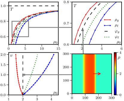
Figure 16: Phase diagrams in the RMFM. The lines $\varphi_{g}$ and $\varphi_{\ell}$ are the spinodal lines denoting the limit of linear stability of homogeneous profiles. The lines $\rho_{g}$ and $\rho_{\ell}$ are coexistence lines that limit the domain of existence of phase-separated profiles. Top row: temperature/density ensemble. The right plot is a zoom of the region delimited by the grey rectangle. $D=r=v=1$. Bottom left: velocity/density ensemble. $D=r=1$, $\beta=1.5$. Bottom right: 2d snapshot of the density field in the phase coexistence region. Its position in the phase diagrams is indicated by the grey squares. $D=r=v=1$, $\beta=1.5$ and $\rho_{0}=2.1$.

Close to the critical point at $\beta=1$,

$$\varphi_{\ell}=\varphi_{g}+\frac{r}{2\alpha}+{\cal O}(\beta-1)$$ (35)

so that $\varphi_{\ell}$ and $\varphi_{g}$ both diverge, while their difference remains constant. Close to the $v=0$ critical point, we obtain

$$\varphi_{\ell}=\varphi_{g}+\frac{rv}{\sqrt{8D\alpha}(\beta-1)}+{\cal O}(v^{2})$$ (36)

so that $\varphi_{\ell}\to\varphi_{g}$ when $v\to 0$.

The homogeneous solutions are linearly unstable in the density range $[\varphi_{g},\varphi_{\ell}]$. Simulating the RMFM foot1 for such densities yield phase-separated profiles similar to those seen in the AIM, with macroscopic liquid bands travelling in a disordered gas background (see bottom-right panel of fig. 16). The densities in the gas and liquid parts of the profiles remain constant as $\rho_{0}$ is varied; they thus give access to the coexistence lines $\rho_{g}$ and $\rho_{\ell}$.

The phase diagrams of the RMFM in the temperature/density and velocity/density ensembles shown in Fig. 16 are qualitatively similar to those of the AIM, with an asymptote at $T=1$ when $\rho_{0}\to\infty$ in the ($T$, $\rho_{0}$) plane, and a critical point at $v=0$ in the ($v$, $\rho_{0}$) plane. As before, the coexistence lines $\rho_{g}$ and $\rho_{\ell}$ delimit the domain of existence of phase-separated solutions; they can now be complemented by the spinodals $\varphi_{g}$ and $\varphi_{\ell}$ which mark the loss of linear stability of homogeneous disordered and order phases, respectively.

The hysteresis loops observed in the RMFM (see Fig. 17) are similar to those found in the microscopic model (see Fig. 9 and 4). Starting at low density in the gaseous phase and increasing density the system stays in the gas phase until it becomes unstable at $\rho_{0}=\varphi_{g}$, where it phase separates. Increasing again the density, the liquid fraction increases linearly until the liquid almost fills the system. As in the AIM, the finite widths of the interfaces set a minimum and a maximum size for a domain, hence preventing liquid bands from completely filling the system. This results in a discontinuous jump of the liquid fraction close to the binodals, whose height vanishes as the system size diverges (see Fig. 17, right panel). The main difference with the hysteresis loops observed for the AIM is that, given the absence of noise in the RMFM, there is no nucleation and the system phase-separates only when the spinodal densities are reached.

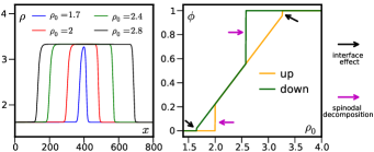
Figure 17: Hysteresis loops in the RMFM. Left: Density profiles along the loop as $\rho_{0}$ is varied. Right: Evolution of the liquid fraction $\phi$ upon changing continuously $\rho_{0}$. Parameters: $\beta=1.5$, $D=v=r=1$, $L=800$.

IV.4 Control parameters

To determine how many independent control parameters are needed to describe the behavior of the RMFM, we recast Eqs. (30) and (31) in dimensionless form. To do so, we first have to introduce back the rate $\gamma$ which appeared in the definition of the flipping rates (1) and that we have taken equal to one until now. Introducing the dimensionless variables and constants

$$t=\hat{t}/\gamma,\>x=\sqrt{\frac{D}{\gamma}}\hat{x},\>\rho=r\hat{\rho},\>m=r\hat{m},\>v^{2}=\gamma D\hat{v}^{2}$$ (37)

the refined mean-field equations become

$$\dot{\hat{\rho}} =\hat{\Delta}\hat{\rho}-\hat{v}\partial_{\hat{x}}\hat{m}$$ (38)

$$\dot{\hat{m}} =\hat{\Delta}\hat{m}-\hat{v}\partial_{\hat{x}}\hat{\rho}+\big{[}2(\beta-1-\frac{1}{\rho})m-\alpha\frac{m^{3}}{\rho^{2}}\big{]}$$ (39)

Since $\alpha$ is a function of $\beta$, there are only two external dimensionless control parameters: $\hat{v}$ is a Peclet number comparing the advection speed $v$ and the diffusivity $D$ at the length scale $v/\gamma$ travelled by a particle between two spin flips; $\beta$ which controls the ordering of the system foot2 The average density, which sets an external constraint on the system, constitutes a third independent parameter. Our phase diagrams shown in Fig. 16 thus sample all the relevant parameters of the RMFM.

V Inhomogeneous band profiles

In the previous section we have shown how one can build a refined mean-field model by taking into account the local fluctuations of magnetisations and densities. Numerical simulations of the RMFM exhibit a phenomenology akin to that of the microscopic AIM, confirming the liquid-gas picture of the phase transition. We now focus on the inhomogeneous profiles and show analytically that the RMFM accounts for their shapes and speeds when $\beta\to 1$. Furthermore, the RMFM also correctly predicts the scaling of the width of the critical bands in the vicinity of the critical points $\beta=1$ and $v=0$.

V.1 Propagative solutions

Let us reduce Eqs. (30) and (31) to a single ordinary differential equation. To do so, we first introduce a new coordinate $z=x-ct$ comoving with the liquid band at an unknown speed $c$. In this comoving frame, the stationnary solutions of the RMFM satisfy

$$D \rho^{\prime\prime}+c\rho^{\prime}-vm^{\prime}=0$$ (40)

$$D m^{\prime\prime}+cm^{\prime}-v\rho^{\prime}+2(\beta-1-\frac{r}{\rho})m-\alpha\frac{m^{3}}{\rho^{2}}=0$$ (41)

The RMFM is a finite-density correction to the $\rho=\infty$ mean-field limit and should thus work best for large densities. As we can see on the phase diagram shown in Fig 5, the densities $\rho_{\ell}$ and $\rho_{g}$ diverge as $\beta\to 1$, as do $\varphi_{g}$ and $\varphi_{\ell}$ (see Eqs. (34) and (35)). Furthermore, one can check that $\rho_{\ell}-\rho_{g}$ remains finite in this limit, as does $m_{\ell}$ (see Fig. 18). Close to $\beta=1$, we can thus expand Eq. (41) in power of $\epsilon=m/\varphi_{g}\sim\delta\rho/\varphi_{g}$, where $\delta\rho\equiv(\rho-\varphi_{g})$, to get

$$0=Dm^{\prime\prime}+cm^{\prime}-v\delta\rho^{\prime}+\frac{2rm\delta\rho}{\varphi_{g}^{2}}-\alpha\frac{m^{3}}{\varphi_{g}^{2}}$$ (42)

Besides, Eq. (40) can be solved iteratively to obtain $\rho(z)$ in terms of $m(z)$ and its derivatives

$$\rho(z)=\rho_{g}+\frac{v}{c}m(z)+\frac{v}{c}\sum_{k=1}^{\infty}\Big{(}-\frac{D}{c}\Big{)}^{k}\frac{d^{k}m(z)}{dz^{k}}$$ (43)

where $\rho_{g}$ is an integration constant that equals the density in the gas phase at coexistence, since $\rho(z)=\rho_{g}$ where $m=0$. Again, the RMFM should work best close to the critical points, where the width of band fronts diverge (see Fig. 11), we can thus expect the development (43) to rapidly converge in this limit and retain only

$$\rho(z)=\rho_{g}+\frac{v}{c}m(z)-\frac{Dv}{c^{2}}m^{\prime}(z)+\frac{vD^{2}}{c^{3}}m^{\prime\prime}(z)$$ (44)

At second order in $\epsilon$, Eqs (42) and (44) then reduces to

$$\hat{D}m^{\prime\prime}+(a_{0}-a_{1}m)m^{\prime}-b_{1}m+b_{2}m^{2}-b_{3}m^{3}=0$$ (45)

where we have introduced the positive constants

$$D =D(1+\frac{v^{2}}{c^{2}}),\quad a_{0}=c\big{(}1-\frac{v^{2}}{c^{2}}\big{)},\quad a_{1}=\frac{4Dvr}{(c^{2}+v^{2})\varphi_{g}^{2}}$$ (46)

$$b_{1} =2r\frac{\varphi_{g}-\rho_{g}}{\varphi_{g}^{2}},\quad b_{2}=\frac{2rv}{c\varphi_{g}^{2}},\quad b_{3}=\frac{\alpha}{\varphi_{g}^{2}}$$

We then look for propagating solutions made of two fronts, connecting an ordered liquid band at $\rho_{\ell}$, $m_{\ell}$ to a disordered gas background at $\rho_{g}$, $m_{g}=0$. Precisely, we look for propagating fronts given by:

$$m(z)=\frac{m_{\ell}}{2}\left[1+\tanh(kz)\right]$$ (47)

To describe phase-separated domains, we need two front solutions, an ascending front $m_{a}(z)$ with $k_{a}>0$ and a descending front $m_{d}(z)$ with $k_{d}<0$, with the same speed $c$, density $\rho_{g}$ and magnetization $m_{\ell}$. Since the term $(a_{0}-a_{1}m)m^{\prime}$ breaks the symmetry of the equations under $(m,c)\to(-m,-c)$ the fore and rear fronts need not be the same, so that $|k_{a}|\neq|k_{d}|$ in general.

The complete solution, specified by ($c$, $\rho_{g}$, $m_{\ell}$, $k_{a/d}$) can be obtained by injecting the Ansatz (47) into Eq. (45). Using the equality $\tanh^{\prime}(kx)=k-k\tanh^{2}(kx)$, the l.h.s. of Eq. (45) then yields a third order polynomial in $\tanh(kx)$ whose coefficients all have to vanish. Tedious but straightforward algebra then gives

$$c =v\Big{(}1+\frac{8r^{2}D}{3\alpha v^{2}\varphi_{g}^{2}}\Big{)}^{\frac{1}{4}}$$ (48)

$$m_{\ell} =\frac{4rv}{3\alpha c}$$

$$\rho_{g} =\varphi_{g}-\frac{4rv^{2}}{9\alpha c^{2}}$$

$$k_{a/d} =-\frac{c\gamma_{-}}{4D\gamma_{+}}\Big{[}1\pm\sqrt{1+\frac{4\gamma_{+}^{3}}{3}+\frac{\gamma_{+}^{3}\alpha v^{2}\varphi_{g}^{2}}{2Dr^{2}}}\Big{]}$$

where $\gamma_{\pm}\equiv 1\pm\frac{v^{2}}{c^{2}}$.

The solution is thus completely determined, the density and magnetization profiles being given by Eq. (47) and (44) respectively.

V.2 Close to the $\beta=1$ critical point

At leading orders when $\beta\to 1$, the propagating fronts are characterized by

$$\rho_{g} =\varphi_{g}-\frac{4r}{9\alpha}; \rho_{\ell}=\varphi_{g}+\frac{8r}{9\alpha};$$ (49)

$$m_{\ell} =\frac{4r}{3\alpha}; c=v+\frac{2D(\beta-1)^{2}}{3v\alpha};$$

$$k_{a} =\frac{\beta-1}{3\sqrt{D\alpha}}-\frac{(\beta-1)^{2}}{6v\alpha}; k_{d}=-\frac{\beta-1}{3\sqrt{D\alpha}}-\frac{(\beta-1)^{2}}{6v\alpha};$$

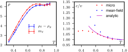
Figure 18: Left: The magnetization $m_{\ell}$ in the liquid band and $\rho_{\ell}-\rho_{g}$ at phase-coexistence, measured in the microscopic simulations, converge to the same constant when $\beta\to 1$ as predicted by the analytical solution. Parameters: $D=1$, $\varepsilon=0.9$, $L=400$ for the microscopic simulations. $r=v=D=1$, $L=400$ for the RMFM. Right: velocity $c$ of a liquid band propagating in a gas background. As $\beta\to 1$, $c\to v$ in the microscopic model, in 1d simulation of the RMFM (31), and in the analytical solution.

Some comments are in order. First, the two coexistence lines $\rho_{g}$ and $\rho_{\ell}$ diverge as $\beta\to 1$, as do the spinodals $\varphi_{g}$ and $\varphi_{\ell}$, while their difference and the magnetization $m_{\ell}$ converge to finite constants. This behavior, which is in line with simulations of the microscopic model (see Fig. 18), legitimates the expansion of (41) in powers of $m/\varphi_{g}$ and $\delta\rho/\varphi_{g}$.

Then, we can check the validity of the gradient expansion by comparing two successive terms in Eq. (43). When $\beta\to 1$, we have

$$\frac{\left(\frac{D}{c}\right)^{k+1}\frac{d^{k+1}m}{dy^{k+1}}}{\left(\frac{D}{c}\right)^{k}\frac{d^{k}m}{dy^{k}}}\sim\frac{D}{c}k_{a/d}\sim(\beta-1)$$ (50)

so that our approximation becomes exact when $\beta\to 1$.

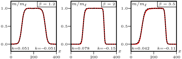
Figure 19: The fore and rear fronts of propagating bands become more asymmetric as $T$ decreases. The shape of the fronts in the microscopic model (red curves) also deviate more and more from the analytical $\tanh$ solution (valid in the limit $\beta\to 1$). Black dashed curves are fits of the rescaled fronts by expression (47), where $k$ is used as a fitting parameter. Parameters: $D=1$, $\varepsilon=0.9$. Fronts are averaged over time and along the vertical direction.

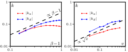
Figure 20: Scaling of the front widths close to the critical points $\beta\to 1$ (left) and $v\to 0$ (right). The data is consistent with the predictions from the RMFM in these limits Eq. (49) and (51) both for the scaling of $k_{a/d}$ and for the asymmetry between the ascending and descending fronts. $\varepsilon=0.9$ (left), $\beta=1.9$ (right) and $D=1$.

The front solutions account for a number of interesting features of the propagating liquid bands. First, the front speed $c$ is generally larger than $v$, the maximal mean speed of a single spin. This may seem surprising until one realizes that the front propagation is due both to the spins in the liquid band hopping forward and to the “conversion” of disordered sites into ordered ones at the level of the fore front. There is thus a FKPP-like contribution vanSaarlosEPL2003 to the speed of a band, which allows $c$ to be larger than $v$. Interestingly, despite the approximations made in deriving the RMFM, the behavior of $c/v$ as $\beta\to 1$ coincides exactly with what is observed in microscopic simulations of the AIM (see Fig. 18).

Regarding the propagating fronts, the analytical solution predicts $|k_{a}|<|k_{d}|$, i.e., that the descending (fore) front is steeper than the ascending (rear) front. The asymmetric term being subleading as $\beta\to 1$, the fore and rear fronts become more and more symmetric as $\beta\to 1$. This is consistent with the microscopic model: In Fig. 19, we show that the fronts are well described by two symmetric $\tanh$ functions close to $\beta=1$. As the temperature decreases, the fronts first remain well approximated by hyperbolic tangents, but with different widths $k_{a}\neq k_{d}$, before their functional form deviates from the $\tanh$ solution (see Fig. 19).

Let us now be slighlty more quantitative and compare the scalings of the front widths in the AIM with the prediction of our analytical solution (49). In the microscopic model, we fitted the fronts of phase-separated profiles by the hyperbolic tangent solutions (47) to extract their width. Although data is hard to obtain close to critical points, because $m/\rho\to 0$, the measures are consistent with the analytical predictions. As shown in Fig. 20, $k_{a/d}\sim(\beta-1)$ when $\beta\to 1$. One can also see that in this limit the two fronts become symmetric, i.e., $k_{a}\to k_{d}$. The size of the inferfaces, inversely proportional to $k_{a/d}$, can be linked to the size of the critical nucleus. As explained in sec. III.4, a liquid domain can form only if the excess number of particles with respect to the gas is sufficient to create a band of minimal size $L_{c}$. As a first approximation, this minimal size is set by the size of the interfaces so that we expect $L_{c}\sim 1/k_{a}+1/k_{d}$. Indeed, the same scalings are observed for $L_{c}$ as for $1/k_{a/d}$ as shown in Fig. 11.

V.3 Close to the $v=0$ critical points

While our approach was derived to work close to the critical point at $\beta=1$, the front solution still predicts many correct scalings close to the $v=0$ critical points. There, the propagating bands are characterized by

$$\rho_{g}=\varphi_{g}-\frac{\sqrt{2}rv}{3(\beta-1)\sqrt{3D\alpha}}$$ (51)

$$\rho_{\ell}=\varphi_{g}+\frac{\sqrt{8}rv}{3(\beta-1)\sqrt{3D\alpha}}$$

$$m_{\ell}=\left(\frac{32r^{4}}{27(\beta-1)^{2}\alpha^{3}D}\right)^{1/4}\sqrt{v}$$

$$c=\left(\frac{8D(\beta-1)^{2}}{3\alpha}\right)^{1/4}\sqrt{v}$$

$$k_{a}=\sqrt{\frac{(\beta-1)}{12D\sqrt{6D\alpha}}}(\sqrt{7}-\sqrt{3})\sqrt{v}$$

$$k_{d}=\sqrt{\frac{(\beta-1)}{12D\sqrt{6D\alpha}}}(-\sqrt{7}-\sqrt{3})\sqrt{v}$$

Again, the two coexisting densities merge with the spinodal lines at $v=0$ while the magnetization in the liquid vanishes, hence justifying the expansion of Eq. (41) in powers of $m/\varphi_{g}$ and $\delta\rho/\varphi_{g}$. While gradients are again expected to vanish as $v\to 0$, the expansion of $\rho$ in derivatives of $m$ includes a diverging prefactor $(D/c)^{k}\sim 1/v^{k/2}$ at the $k^{\text{th}}$ order. The comparison of two successive terms in the expansion (44) then yields

$$\frac{\left(\frac{D}{c}\right)^{k+1}\frac{d^{k+1}m}{dy^{k+1}}}{\left(\frac{D}{c}\right)^{k}\frac{d^{k}m}{dy^{k}}}\sim\frac{D}{c}k_{a/d}\sim{\cal O}(1)$$ (52)

Thus, in this limit, the series may still converge but the ratios between two consecutive terms do not vanish as $v\to 0$ and we cannot completely neglect higher order gradients. Nevertheless, as shown in Fig. 20, the analytical solution correctly predicts that the asymmetry between the fore and rear fronts does not disappear in the $v\to 0$ limit. It also correctly predicts the scaling of the front widths $k_{a/d}\sim\sqrt{v}$ and thus the scaling of the critical nucleus in this regime.

Beyond accounting for the shape of the phase diagram and the liquid-gas nature of the transition, the RMFM can thus correctly predict the shape of the band, their speed and the scaling of the critical nucleus in the vicinity of the critical points. In order to get a more quantitative agreement between the RMFM and the microscopic model, beyond the estimation of the unknown parameter $r$, one would probably needs to account for the correlations between $m$ and $\rho$. Apart from quantitative corrections, these correlations however do not seem to play any role in controling the structure of the phase transition and most features of the propagating bands. Interestingly, symmetric hyperbolic tangent front were also observed in hydrodynamic equations for self-propelled rods Peshkov2012 , even though in that case the domains are not moving.

VI Robustness of the results

Let us now discuss how the results presented in the previous sections extend beyond our lattice-gas model with periodic boundary conditions. To do so, we consider the case of closed boundary conditions in section VI.1 and study an off-lattice version of the AIM in section VI.2.

VI.1 Closed boundary conditions

Since the ordered liquid domains always span the whole system in the vertical direction and propagates periodically in the horizontal direction, one could think that their existence and stability relies on the use of periodic boundary conditions. To check this, we simulated the AIM in closed boxes. We tried different conditions at the edges of the box: When particles hit a wall, their spins were either flipped, randomized, or left unaltered.

The same behavior was observed in all cases. First, one notice a small accumulation of particles close to the wall, which is typical of self-propelled particles Elgeti2009EPL . Then, the system shows the same type of travelling bands as with periodic boundary conditions, with a macroscopic phase-separation between a liquid domain and a gaseous disordered background (see Fig. 21, top). When the liquid domain reaches a boundary, it accumulates close to the wall until its magnetisation flips, and crosses back the system in the other direction. This leads to the bouncing wave shown on Fig. 21 (bottom), which is reminiscent of what is observed experimentally for the collective motion of colloidal rollers (see supplementary movies of BartoloNature ).

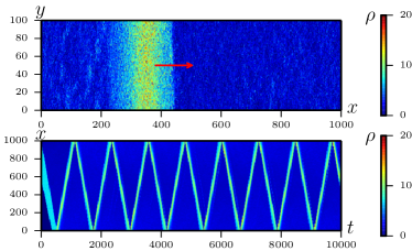
Figure 21: Active Ising model with closed boundary conditions. Top: snapshot of the density field. Bottom: space-time graph (averaged in the y-direction) showing the liquid domain bouncing back and forth in the box. Parameters: $\beta=1.9$, $\rho_{0}=3$, $D=1$, $\varepsilon=0.9$. See supplementary movies in SI .

VI.2 Off-lattice version

To show that the phenomenology of the AIM does not rely on the spatial discreteness of this lattice gas, we devised an off-lattice version of our model. To do so, we consider $N$ particles in a continuous space of size $L_{x}\times L_{y}$. Each particle carries a spin $\pm 1$, which flips at rate

$$W(s\to-s)=\exp(-\beta\frac{m_{i}}{\rho_{i}})$$ (53)

where the local density $\rho_{i}$ and magnetization $m_{i}$ are computed in disks of radius $1$.

The position of the particle evolves according to the Langevin equation

$${\bf\dot{r}_{i}}=s_{i}v{\bf e_{x}}+\sqrt{2D}\boldsymbol{\eta}$$ (54)

where ${\bf r_{i}}$ and $s_{i}$ are the position and spin of particle $i$ and $\boldsymbol{\eta}$ is a Gaussian white noise of unit variance.

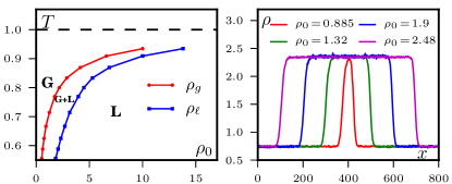
Figure 22: Phase diagram and phase-separated profiles for the off-lattice model showing the same behavior as the lattice model. Parameters: $D=1$, $v=1$ and $\beta=1.6$ for the profiles.

The phenomenology of this model is very similar to that of the AIM; Its phase diagram in the temperature-density ensemble shows the same three regions, with an asymptote at $\beta=1$ as $\rho\to\infty$ (Fig. 22, left). As in the lattice model, only the liquid fraction changes when $\rho_{0}$ is increased at fixed temperature as shown in Fig. 22 (right).

VII Discussion and outlook

In this paper we have characterized in detail the transition to collective motion in the 2d active Ising model. For any temperature $T<1$ and self-propulsion velocity $v>0$, there is a finite density range for which the system phase-separates into a polar liquid and a disordered gas. The densities at coexistence do not depend on $T$ or $v$ so that changing the average density only changes the liquid fraction. This is one of the many characteristics shared by the flocking transition of the AIM with the equilibrium liquid/gas transition in the canonical ensemble. Others include metastability, hysteresis, and the existence of critical nuclei. More generally, this analogy suggests that the flocking transition should be seen as a phase-separation transition rather than an order-disorder transition. The fact that the liquid phase is ordered however plays a major role by forbidding a supercritical region, which explains the atypical shape of the phase diagram.

To construct a continuous theory for our model we first noticed that one needs to go beyond a standard mean-field approach. The latter indeed fails to capture the phase separation behavior because it lacks a density dependence of the transition temperature. Retaining part of the fluctuations neglected at the mean-field level then allowed us to derive a refined-mean-field model which accounts for the behavior of the microscopic model qualitatively for all parameter values.

The analytical solution for the phase-separated profile that we derived in sec. V is only one of a two-parameter family of solutions, as shown in Caussin . Although it is the sole propagating solution accounting for phase separation, the mecanism by which it is selected remains to be investigated. This is particularly interesting since, as shown in SolonVMPRL2015 , most of the picture laid out for the AIM remains valid for the Vicsek model, apart from the shape of the bands in the phase separated region. The full phase separation of the AIM is then replaced by a micro-phase separation, something which cannot be explained at the hydrodynamic level and necessit explicit noise terms.

Beyond the sole case of the AIM, we showed that our results are also valid off lattice. We can thus consider the AIM as a representative example of a flocking model with discrete rotational symmetry. Variants with alignment between nearest neighbours, and not simply on-site, also yield similar results.

Our study of the AIM relies on numerical simulations, microscopic derivation and study of hydrodynamic equations. It says little about the universality of the emerging properties of the Active Ising Model and we strongly believe that developing proper field theoretical approaches of the AIM and more general active spin models could shed light on a number of interesting questions. For instance, is the $\epsilon=0$ limit of the AIM in the universality class of model C HohenbergHalperin , which couples a conserved diffusive field and a non-conserved $\phi^{4}$ theory? Then, can one study the divergence of the correlation length of the AIM when approaching the $T=1$ and $v=0$ critical points? What are the corresponding universality classes? These questions will be addressed in future works.

Last, the analogy of the phase transition in the AIM with an equilibrium liquid/gas transition triggers new questions. For example, could we define a mapping, at some level, with an equilibrium system? And would it be possible to change ensemble in this non-equilibrium system, for example desining a grand-canonical ensemble? These questions, if answered, would certainly improve our theoretical understanding of active matter systems.

Appendix A One step beyond mean-field

As shown in section IV.1, the mean-field equations, which neglect all fluctuations and correlations, fail to describe the active Ising model since they predict a continuous phase transition between homogeneous phases. In this appendix we show how one can improve the mean-field approximation. To do so, we take into account the fluctuations of the local magnetisations and densities when computing the dynamics of their first moments $\langle m\rangle$ and $\langle\rho\rangle$.

A.1 Gaussian fluctuations

The simplest assumption that can be made about the fluctuations of $m(x)$ and $\rho(x)$ around their mean values, $\langle m(x)\rangle$ and $\langle\rho(x)\rangle$, is that they are Gaussian. For $m(x)$, this can be seen as resulting from a central limit theorem: In a first approximation, the magnetisation is the sum of many spins fluctuating independently and, indeed, Fig. 23 shows its fluctuations to be well described by a Gaussian. On the contrary, the distribution of the local density is not perfectly Gaussian, as shown in Fig. 23. A better approximation could be obtained by considering a Poisson distribution but, as will be apparent in the following, the first correction to mean-field comes from the fluctuations of $m$ so this would not improve our approximation. Furthermore we believe that, to improve our refined mean-field model, the next step should be to include the correlations between $\rho$ and $m$, that we neglect in the following, and not higher cumulants of the distributions of $\rho$ and $m$.

More formally, the probability to observe a magnetisation $m$ and a density $\rho$ at time $t$ and position $x$ given initial profiles $\rho_{0}(x)$ and $m_{0}(x)$ are assumed to be given by

$${\cal P}(\rho,m,x,t\,|\,\rho_{0},m_{0})={\cal N}(\rho-\bar{\rho},\sigma_{\rho}^{2}){\cal N}(m-\bar{m},\sigma_{m}^{2})$$ (55)

where ${\cal N}(x,\sigma^{2})=e^{-x^{2}/\sigma^{2}}/\sqrt{2\pi\sigma^{2}}$ is the normal distribution and $\bar{\rho}(x,t)$ and $\bar{m}(x,t)$ are the average value of the density and magnetisation fields.

We further assume that the variances of the Gaussian distributions scales linearly with the local density: $\sigma_{m}^{2}=\alpha_{m}\bar{\rho}(x,t)$ and $\sigma_{\rho}^{2}=\alpha_{\rho}\bar{\rho}(x,t)$. Again, the underlying assumption is that the fluctuations of the fields $\rho(x)$ and $m(x)$ arise from the sum of $\rho$ independent contributions. As shown in Fig. 24 this is a rather good approximation in the gas phase, close to the critical point at $\beta=1$, $\rho=\infty$.

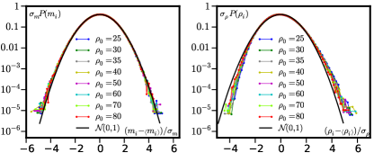
Figure 23: Rescaled probability distributions of local density (left) and magnetisation (right) in the liquid phase at $\beta=1.1$ for different densities. $\mathcal{N}(0,1)$ is the Gaussian distribution with zero mean and unit variance. $D=1$, $\varepsilon=0.9$, $L=100$.

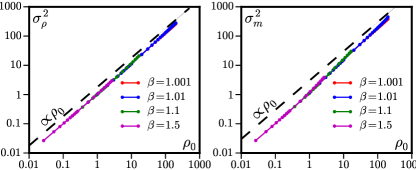
Figure 24: Variance of the distribution of local density (left) and magnetisation (right) in the gas phase compared to a linear scaling. $D=1$, $\varepsilon=0.9$, $L=100$.

A.2 Corrections to mean-field

In deriving hydrodynamic equations from Eq. (18) and (19), the only terms that have to be approximated are the non-linear contributions of the aligning interactions:

$$I=\left\langle 2\rho\sinh\frac{\beta m}{\rho}-2m\cosh\frac{\beta m}{\rho}\right\rangle=\left\langle\sum_{k=0}^{\infty}a_{k}\frac{m^{2k+1}}{\rho^{2k}}\right\rangle$$ (56)

where

$$a_{k}=2\left(\frac{\beta^{2k+1}}{(2k+1)!}-\frac{\beta^{2k}}{(2k)!}\right)$$ (57)

Using the assumption (55), we can compute $I$ as a sum of Gaussian integrals which can all be evaluated by saddle-point approximation in the limit of large $\bar{\rho}$. We first notice that, since we neglect the correlations between $\rho$ and $m$,

$$\left\langle\frac{m^{2k+1}}{\rho^{2k}}\right\rangle=\left\langle m^{2k+1}\right\rangle\left\langle 1/\rho^{2k}\right\rangle$$ (58)

To compute $\left\langle m^{2k+1}\right\rangle$, we first change variables to $u=m-\bar{m}$ so that

$$\left\langle m^{2k+1}\right\rangle =\int_{-\infty}^{+\infty}dm\,m^{2k+1}{\cal N}(m-\bar{m},\alpha_{m}\bar{\rho})$$

$$=\int_{-\infty}^{+\infty}du\,(u+\bar{m})^{2k+1}{\cal N}(u,\alpha_{m}\bar{\rho})$$ (59)

We then expand in powers of $u$ and compute the corresponding Gaussian integrals

$$\left\langle m^{2k+1}\right\rangle =\int_{-\infty}^{+\infty}du\sum_{i=0}^{2k+1}\binom{2k+1}{i}u^{i}\bar{m}^{2k+1-i}{\cal N}(u,\alpha_{m}\bar{\rho})$$

$$=\sum_{j=0}^{k}\binom{2k+1}{2j}\frac{\Gamma(j+1/2)}{\sqrt{\pi}}(2\alpha_{m}\bar{\rho})^{j}\bar{m}^{2k+1-2j}$$ (60)

Let us now evaluate the terms $\left\langle\rho^{-2k}\right\rangle$. First, the integral

$$\left\langle\rho^{-2k}\right\rangle=\int_{0}^{+\infty}d\rho\,\rho^{-2k}{\cal N}(\rho-\bar{\rho},\alpha_{\rho}\bar{\rho})$$ (61)

is divergent because of the $\rho=0$ lower limit. This is a simple discretisation problem which can be bypassed by introducing a cut-off $\zeta$ at small density. For large $\bar{\rho}$, the integrals will be dominated by large values of $\rho$ so this cut-off does not play any role in the following. Changing variable to $s=(\rho-\bar{\rho})/\bar{\rho}$, we find

$$\left\langle\rho^{-2k}\right\rangle=\frac{\bar{\rho}^{\,\frac{1}{2}-2k}}{\sqrt{2\pi\alpha_{\rho}}}\int_{\frac{\zeta}{\bar{\rho}}-1}^{+\infty}ds\,(1+s)^{-2k}e^{-\bar{\rho}\frac{s^{2}}{2\alpha_{\rho}}}$$ (62)

This integral can now be approximated by an asymptotic saddle-point expansion. In the limit of large $\bar{\rho}$, the integral is dominated by $s\simeq 0$. The lower limit of the integral $\frac{\zeta}{\bar{\rho}}-1\simeq-1$ can thus be extended to $-\infty$ harmlessly and one can expand $(1+s)^{-2k}$ to get the asymptotic expansion

$$\left\langle\rho^{-2k}\right\rangle =\frac{\bar{\rho}^{\,\frac{1}{2}-2k}}{\sqrt{2\pi\alpha_{\rho}}}\sum_{i=0}^{2N}\binom{2k+i-1}{i}\int_{-\infty}^{+\infty}ds\,(-s)^{i}e^{-\bar{\rho}\frac{s^{2}}{2\alpha_{\rho}}}$$ (63)

$$\qquad\qquad+{\cal O}(\bar{\rho}^{\,-2N-2k-1/2})$$

All the odd contributions vanish by symmetry. Changing variable to $\omega=\bar{\rho}s^{2}/(2\alpha_{\rho})$, one recognises the integral form of a $\Gamma$ function and finally

$$\left\langle\rho^{-2k}\right\rangle =\sum_{j=0}^{N}\binom{2k+2j-1}{2j}\frac{\Gamma(j+\frac{1}{2})}{\sqrt{\pi}}2^{j}\alpha_{\rho}^{j}\bar{\rho}^{\,-j-2k}$$ (64)

$$\qquad\qquad+{\cal O}(\bar{\rho}^{\,-2k-2N-1})$$

Putting everything together, we obtain

$$I=\sum_{k=0}^{\infty}\sum_{i=0}^{k}\sum_{j=0}^{N}\Big{[}a_{k}b_{i,k}c_{j,k}\frac{\bar{m}^{1+2k-2i}}{\bar{\rho}^{\,2k+j-i}}+{\cal O}(\frac{1}{\bar{\rho}^{\,1+N+2k-i}})\Big{]}$$ (65)

where

$$b_{i,k} =\binom{2k+1}{2i}\frac{2^{i}\Gamma(i+1/2)}{\sqrt{\pi}}\alpha_{m}^{i}$$ (66)

$$c_{j,k} =\binom{2k+2j-1}{2j}\frac{2^{j}\Gamma(j+1/2)}{\sqrt{\pi}}\alpha_{\rho}^{j}$$ (67)

Keeping only the dominant terms and reordering the sum in increasing powers of $m$ yields

$$I=\sum_{n=0}^{\infty}\frac{\bar{m}^{1+2n}}{\bar{\rho}^{\,2n}}\Big{[}\sum_{i=0}^{N}\sum_{j=0}^{N-i}\frac{a_{n+i}b_{i,n+i}c_{j,n+i}}{\bar{\rho}^{\,j+i}}+{\cal O}(\frac{1}{\bar{\rho}^{\,1+N}})\Big{]}$$ (68)

Expanding up to $m^{3}$ and $1/\bar{\rho}^{2}$, we finally obtain

$$I\simeq 2\big{(}\beta-1-\frac{r}{\bar{\rho}}-\frac{r_{2}}{\bar{\rho}^{2}}\big{)}\bar{m}-\alpha\frac{\bar{m}^{3}}{\bar{\rho}^{2}}$$ (69)

where

$$\alpha =-a_{1}=\beta^{2}(1-\frac{\beta}{3})$$ (70)

$$r =-\frac{a_{1}b_{1,1}c_{0,1}}{2}=\frac{3\alpha\alpha_{m}}{2}$$ (71)

$$r_{2} =3\beta^{2}(\beta-3)\alpha_{m}\alpha_{\rho}+\frac{\beta^{4}}{4}(\beta-5)\alpha_{m}^{2}$$ (72)

In practice, we take $r_{2}=0$ in the RMFM since the first order correction $r/\bar{\rho}$ suffices to account for the phenomenology of the AIM. Expanding (68) to higher orders is not sufficient to get a quantitative agreement between microscopic simulations and our refined mean-field model, probably because the most important correction to (69) would involve correlations between $m$ and $\rho$. As we show in section IV, however, this first correction to mean-field is sufficient to capture the physics of the model.

Appendix B Linear stability analysis

The mean-field and refined mean-field equations read

$$\dot{\rho} =D\Delta\rho-v\partial_{x}m$$ (73)

$$\dot{m} =D\Delta m-v\partial_{x}\rho+2m\mu-\alpha\frac{m^{3}}{\rho^{2}}$$ (74)

where $\mu=\beta-1-r/\rho$ and $r=0$ for the mean-field equations. These equations admit three steady homogeneous solutions $\rho(x,t)=\rho_{0}$, $m(x,t)=m_{0}$. A disordered solution with $m_{0}=0$ that exists for all $\rho_{0}$ and $\beta$, and two ordered solutions

$$m_{0}=\pm\rho_{0}\sqrt{\frac{2\mu}{\alpha}}$$ (75)

that exist only when $\mu>0$.

B.1 Stability of the disordered profile

Let us consider a small perturbation around the disordered profile, $m({\bf r},t)=\delta m({\bf r},t)$, $\rho({\bf r},t)=\rho_{0}+\delta\rho({\bf r},t)$. Going into Fourier space,

$$\delta\rho=\int_{-\infty}^{\infty}\!\!\!\!dx\int_{-\infty}^{\infty}dy\,\delta\rho({\bf q},t)e^{-i(q_{x}x+q_{y}y)}$$ (76)

and linearizing Eqs. (73) and (74), one finds

$$\partial_{t}\begin{pmatrix}\delta\rho\\ \delta m\end{pmatrix}=\begin{pmatrix}-D|q|^{2}&-iq_{x}v\\ -iq_{x}v&-D|q|^{2}+2\mu_{0}\end{pmatrix}\begin{pmatrix}\delta\rho\\ \delta m\end{pmatrix}$$ (77)

where we noted $\mu_{0}=(\beta-1-r/\rho_{0})$. The eigenvalues of the 2x2 matrix are

$$\lambda_{\pm}=-D(q_{x}^{2}+q_{y}^{2})+\mu_{0}\pm\sqrt{\mu_{0}^{2}-v^{2}q_{x}^{2}}$$ (78)

The profile is linearly unstable if one of these eigenvalues has a positive real part. Clearly, the sign of $\mu_{0}$ controls the stability: the disordered profile is unstable to long wavelength perturbations when $\beta>1$ and $\rho_{0}>\varphi_{g}=r/(\beta-1)$ and stable otherwise. This gives the first spinodal line $\varphi_{g}$ in Fig. 16.

B.2 Stability of the ordered profile

Linearizing the dynamics of a small perturbation around the ordered profile $m({\bf r},t)=m_{0}+\delta m({\bf r},t)$, $\rho({\bf r},t)=\rho_{0}+\delta\rho({\bf r},t)$ gives

$$\partial_{t}\begin{pmatrix}\delta\rho\\ \delta m\end{pmatrix}=\begin{pmatrix}-D|q|^{2}&-iq_{x}v\\ -iq_{x}v+\frac{m_{0}}{\rho_{0}}(\frac{2r}{\rho_{0}}+4\mu_{0})&-D|q|^{2}-4\mu_{0}\end{pmatrix}\begin{pmatrix}\delta\rho\\ \delta m\end{pmatrix}$$ (79)

and the eigenvalues now read

$$\lambda_{\pm}=-D(q_{x}^{2}+q_{y}^{2})-2\mu_{0}\pm\sqrt{4\mu_{0}^{2}-v^{2}q_{x}^{2}-\frac{2im_{0}q_{x}v(r+2\mu_{0}\rho_{0})}{\rho_{0}^{2}}}$$ (80)

Equation (80) shows $q_{y}$ to have a purely stabilizing effect; Taking $q_{y}=0$ thus does not affect the conclusions about the stability of the system. Computing numerically $\Re(\lambda_{\pm})$ we observe (Fig. 25) that for small but positive $\mu_{0}$, $\Re(\lambda_{\pm})>0$ at long wave-length. The value of $\mu_{0}$ at which the system becomes stable can be determined analytically as the point where $\partial_{qx}^{2}\Re(\lambda_{\pm})(q_{x}=0)$ changes sign (the first derivative being zero at $q_{x}=0$). This yields the second spinodal line shown in Fig. 16

$$\varphi_{\ell}=\varphi_{g}\frac{v\sqrt{\alpha\left(v^{2}\kappa+8D(\beta-1)^{2}\right)}+v^{2}\kappa+8D\alpha(\beta-1)}{2v^{2}\kappa+8D\alpha(\beta-1)}$$ (81)

where $\kappa=2+\alpha-2\beta$.

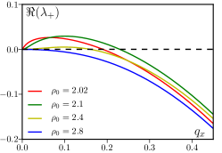
Figure 25: Real part of the largest eigenvalue $\lambda_{+}$ related to the stability of the ordered profile $m=m_{0}$. of Eq. (80) for $\beta=1.5$, $D=r=v=1$ and $q_{y}=0$. Ordered profiles exist for all $\rho_{0}\geq\varphi_{g}=2$ but are unstable for $\varphi_{g}\leq\rho_{0}\leq\varphi_{\ell}$ (red, green and yellow curves) and stable only for $\rho_{0}\geq\varphi_{\ell}$ (blue curve). For the parameters considered here $\varphi_{\ell}=2.598$.

References

- (1) M. Ballerini, N. Cabibbo, R. Candelier, A. Cavagna, E. Cisbani, I. Giardina, V. Lecomte, A. Orlandi, G. Parisi, A. Procaccini, M. Viale, V. Zdravkovic, Proc. Natl. Acad. Sci. USA 105 1232 (2008)
- (2) Ch. Beccoa, N. Vandewallea, J. Delcourtb and P. Poncinb, Physica A, Volume 367, 15 July 2006, Pages 487–493
- (3) D. S. Calovi et al, New J. Phys. 16 (2014)
- (4) E. B. Steager, C.-B. Kim, M. J. Kim. Physics of Fluids, 20(7):073601, 2008.
- (5) F. Peruani, J. Starruss, V. Jakovljevic, L. Sogaard-Andersen, A. Deutsch, M. Bär, Phys. Rev. Lett. 108, 098102 (2012)
- (6) V. Schaller, C. Weber, C. Semmrich, E. Frey, A. R. Bausch, Nature 467, 73-77 (2010).
- (7) Y. Sumino, K. H. Nagai, Y. Shitaka, D. Tanaka, K. Yoshikawa, H. Chaté, K. Oiwa, Nature 483 448-452 (2012).
- (8) J. Deseigne, O. Dauchot, H. Chaté. Phys. Rev. Lett., 105, 098001 (2010); J. Deseigne et al, Soft Matter 8.20 (2012)
- (9) A. Bricard, J-B. Caussin, N. Desreumaux, O. Dauchot, D. Bartolo, Nature 503, 95–98 (2013)
- (10) Shashi Thutupalli et al 2011 New J. Phys. 13 073021
- (11) T. Vicsek, A. Czirók, E. Ben-Jacob, I. Cohen, O. Shochet, Phys. Rev. Lett. 75, 1226 (1995)
- (12) J. Toner and Y. Tu, Phys. Rev. Lett. 75, 4326 (1995); Phys. Rev. E 58, 4828 (1998); J. Toner, Phys.Rev.E 86, 031918 (2012)
- (13) G. Grégoire, H. Chaté, Phys. Rev. Lett. 92 025702 (2004); H. Chaté, F. Ginelli, G. Grégoire, F. Raynaud, Phys. Rev. E 77 046113 (2008).
- (14) A. P. Solon, H. Chaté, J. Tailleur, Phys. Rev. Lett. 114 068101 (2015)
- (15) S. Mishra, A. Baskaran, M.C. Marchetti. Phys. Rev. E 81, 061916. (2010); A. Gopinath, M.F. Hagan, M.C. Marchetti, A. Baskaran. Phys. Rev. E 85, 061903. (2012)
- (16) C. A. Weber, T. Hanke, J. Deseigne, S. Léonard, O. Dauchot, E. Frey, H. Chaté Phys. Rev. Lett. 110, 208001 (2013)
- (17) F. Peruani, T. Klauss, A. Deutsch, and A. Voss-Boehme, Phys. Rev. Lett. 106, 128101 (2011)
- (18) F. D. C. Farrell, M. C. Marchetti, D. Marenduzzo, and J. Tailleur, Phys. Rev. Lett. 108, 248101 (2012)
- (19) E. Bertin, M. Droz, G. Grégoire, Phys. Rev. E 74 022101 (2006); J. Phys. A 42 445001 (2009)
- (20) T. Ihle, Phys. Rev. E 83, 030901 (2011); T. Ihle, Phys. Rev. E 88, 040303(R) (2013)
- (21) J. Toner, Y. Tu, and S. Ramaswamy, Ann. Phys. (N.Y.) 318, 170 (2005)
- (22) A.P. Solon, J. Tailleur, Phys. Rev. Lett. 111, 078101 (2013)
- (23) J-B Caussin, A. Solon, A. Peshkov, H. Chaté, T. Dauxois, J. Tailleur, V. Vitelli, and D. Bartolo, Phys. Rev. Lett. 112, 148102 (2014)
- (24) C. Domb, R. K. Zia, B. Schmittmann, J. L. Lebowitz. Statistical mechanics of driven diffusive systems. Academic Press, 1995
- (25) M. Kim, S.-C. Park, J. D. Noh. Phys. Rev. E 91 012132 (2015)
- (26) K. R. Pilkiewicz, J. D. Eaves. Phys. Rev. E 89 012718 (2014).
- (27) A.N. Kolmogorov, Math. Ann. 112, 155-160 (1936)
- (28) S. Ngo, A. Peshkov, I.S. Aranson, E. Bertin, F. Ginelli, and H. Chaté, Phys. Rev. Lett. 113, 038302 (2014)
- (29) A. Peshkov, I. S. Aranson, E. Bertin, H. Chaté, F. Ginelli, Phys. Rev. Lett. 109, 268701 (2012)
- (30) F. Thüroff, C. A. Weber, and E. Frey, Phys. Rev. X 4, 041030 (2014)
- (31) A. Czirók, H. Stanley, T. Vicsek, J. Phys. A: Math. Gen. 30 1375 (1997)
- (32) O. J. O’Loan, M. R. Evans, J. Phys. A: Math. Gen. 32 L99 (1999)
- (33) G. Baglietto, E. V. Albano, J. Candia, Interface Focus 2 708-714 (2012).
- (34) K. Binder, Rep. Prog. Phys. 60 487 (1997)
- (35) G. Kamieniarz and H. W. J. Blote, J. Phys. A: Math. Gen. 26 201 (1993)
- (36) F. Ginelli, H. Chaté, Phys. Rev. Lett. 105, 168103 (2010)
- (37) S. Dey, D. Das, and R. Rajesh, Phys. Rev. Lett. 108, 238001 (2012)
- (38) I. S. Aranson et al., Science 320 612 (2008)
- (39) Y. Fily, M. Cristina Marchetti, Phys. Rev. Lett. 108 235702 (2012).
- (40) R. A. Blythe, M. R. Evans, J. Phys. A 40 R333 (2007).
- (41) M. R. Evans, Y. Kafri, K. E. P. Sugden, J. Tailleur, J. Stat. Mech. P06009 (2011)
- (42) P. Weiss, J. de Phys. 6, pp. 661-690 (1907)
- (43) A. Baskaran, M. C. Marchetti, Phys. Rev. E 77, 011920 (2008)
- (44) I. S. Aranson, L. S. Tsimring, Phys. Rev. E 71, 050901(R) (2005)
- (45) W. van Saarloos, Phys. Rep. 386, 29 (2003).
- (46) J. Elgeti, G. Gompper, EPL (Europhysics Letters) 85, 38002 (2009).
- (47) To integrate the PDE of the (refined) mean-field model, we used pseudo-spectral methods, computing the linear terms in Fourier space with implicit time stepping.
- (48) The definition of the Hamiltonian (2) does not contain any coupling constant so that is dimensionless.
- (49) See Supplemental Material at http://www.msc.univ-paris-diderot.fr/~solon/SI_ising2d
- (50) P. C. Hohenberg and B. I. Halperin, Rev. Mod. Phys. 49, 435 (1977)