Inflationary Predictions and Moduli Masses
Kumar Das^∗, Koushik Dutta^∗, Anshuman Maharana^†

^∗Theory Division,
Saha Institute of Nuclear Physics,
1/AF Salt Lake,
Kolkata - 700064, India.
^†Harish Chandra Research Intitute,
Chattnag Road, Jhunsi,
Allahabad - 211019, India.

A generic feature of inflationary models in supergravity/string constructions is vacuum misalignment for the moduli fields. The associated production of moduli particles leads to an epoch in the post-inflationary history in which the energy density is dominated by cold moduli particles. This modification of the post-inflationary history implies that the preferred range for the number of e-foldings between horizon exit of the modes relevant for CMB observations and the end of inflation $(N_{k})$ depends on moduli masses. This in turn implies that the precision CMB observables $n_{s}$ and $r$ are sensitive to moduli masses. We analyse this sensitivity for some representative models of inflation and find the effect to be highly relevant for confronting inflationary models with observations.

1 Introduction

Precision measurements of the cosmic microwave background (CMB) have put the inflationary paradigm as the leading candidate for a theory of early universe cosmology. The data is in perfect agreement with the basic qualitative predictions of inflation i.e. an approximately scale invariant and adiabatic power spectrum. Upcoming observations are expected to probe the CMB with an even greater accuracy and provide us information regarding the strengths of the tensor to scalar ratio and non-gaussianities.

On the theoretical front, there are many challenges. The inflationary slow roll conditions are ultraviolet sensitive; we should embed models of inflation in a quantum theory of gravity. In this light, an important direction of research is study of the effects that can arise as a result of ultraviolet completion of inflationary models. String theory provides a setting where one can hope to carry out a systematic study of such effects.

A generic feature of supergravity/string models are the moduli fields. The vacuum expectation value of moduli fields set the strength and form of the low energy effective action of string models, hence moduli fields play a central role in string phenomenology. In the context of inflationary model building, a knowledge of the moduli potential and the couplings between the inflaton and the moduli are necessary to address the $\eta$ problem. There has been an extremely useful interplay between studies of moduli stabilisation and inflationary model building in string theory, see for e.g. [1, 2, 3]. In this paper, we will examine the sensitivity of precision CMB observables – the spectral tilt $(n_{s})$ and the tensor to scalar ratio $(r)$ to the mass of the lightest modulus field.

Given a model of inflation, one can express $n_{s}$ and $r$ in terms of the number of e-foldings between horizon exit of the modes relevant for CMB observations and the end of inflation $(N_{k})$. Predictions for $n_{s}$ and $r$ are then made by using the “preferred range” of $N_{k}$ (usually taken to be 50 to 60) in these formulae. The preferred range for $N_{k}$ is determined as follows – the inflationary paradigm relates the strength of temperature fluctuations in the CMB to the energy density of the universe at the time of horizon exit $(\rho_{k})$ and the tensor to scalar ratio $(r)$. Thus, in the context of inflationary models the measurement of the temperature fluctuations of the CMB determines the energy density of the universe at the time of horizon exit (modulo $r$). The CMB measurements via determination of the Hubble constant also provide us with the energy density of the universe today $(\rho_{0})$. This implies a consistency condition for any theoretical proposal for the history of the universe between the time of horizon exit of the modes relevant for CMB observations and today - the “early time” energy density $\rho_{k}$ should precisely evolve to the energy density today $\rho_{0}$. In the standard model of cosmology, the history of the universe between horizon exit and today consists of the following epochs - inflation, reheating, radiation domination and matter domination. Applying the above mentioned consistency condition to this cosmological timeline, along with the assumption that the reheating epoch is generic gives $N_{k}$ to be in the range of 50 to 60 (see for e.g. [4]).

From the very early days of inflationary model building in supergravity it was realised that a generic implication of having moduli fields is a non-standard post-inflationary cosmological timeline [5, 6, 7, 8, 9, 10] (often referred to as the modular cosmology timeline). The modular cosmology timeline sets in whenever there is a modulus of post-inflationary mass $(m_{\varphi})$ below the Hubble scale during inflation. Such a modulus gets displaced from its post-inflationary minimum due to vacuum misalignment during the inflationary epoch. This misalignment is responsible for the non-standard post-inflationary cosmological timeline (which we will describe in detail in section 2). The distinguishing feature of this timeline is an epoch in which the energy density of the universe is dominated by cold moduli particles produced as a result of the misalignment. The duration of this epoch is governed by the lifetime of the modulus (which is typically set by the mass of the modulus as moduli decay via their Planck suppressed interactions). The universe reheats for a second time with the decay of the modulus (the first reheating being associated with the decay of the inflaton), after which the history is thermal . Reference [11] derived the consistency condition described in the previous paragraph for the modular cosmology timeline. With the assumption of generality on the reheating epoch, the consistency condition turns out to be a relationship between $N_{k}$ and the number of e-foldings of the universe during the epoch in which the cold moduli particles dominate the energy density $(N_{\rm mod})$

$$50\lesssim N_{k}+{1\over 4}N_{\rm mod}\lesssim 60.$$ (1.1)

In this paper our goal is to explore in detail the phenomenological implications of the above relation. The relation can be thought of as implying a shift in the central value of the preferred number of e-foldings

$$55\to 55-{1\over 4}N_{\rm mod}.$$ (1.2)

$N_{\rm mod}$ can be expressed in terms of the mass of the lightest modulus $(m_{\varphi})$ in the compactification and the “initial displacement” of the modulus in Planck units $(Y)$, that occurs as a result of misalignment [11]

$$N_{\rm mod}\approx{4\over 3}\ln\bigg{(}{\sqrt{16\pi}M_{\rm pl}Y^{2}\over m_{\varphi}}\bigg{)}.$$ (1.3)

Typically, in supergravity models the initial displacement $Y$ is of $\mathcal{O}(1)$ [13, 14, 15, 16, 17]. Thus the shift in the central value of $N_{k}$ is essentially determined by the mass of the modulus.

Recall that given a model of inflation, the predictions for $n_{s}$ and $r$ are made by expressing $n_{s}$ and $r$ in terms of $N_{k}$; and then making use of the preferred range for $N_{k}$ in these expressions. As discussed above, in supergravity models the central value of the preferred range for $N_{k}$ depends on the mass of the lightest modulus. Hence, the predictions for $n_{s}$ and $r$ of an inflationary model are sensitive to its embedding into a supergravity/string compactification. In this paper, we will study this sensitivity for some representative models of inflation ($m^{2}\chi^{2}$ [18], axion monodromy [19], natural inflation [20] and the Starobinsky model [21]). Motivated by the varied spectra of phenomenologically viable supergravity models we will treat the mass of the lightest modulus $(m_{\varphi})$ as a parameter. At any given value of $m_{\varphi}$, the preferred range of $N_{k}$ can be computed using (1.2) and (1.3), the predictions for $n_{s}$ and $r$ can then be made.

We analyse our results in the context of planck 2015 data [22]. The implications are very interesting – the changes in inflationary predictions can significantly affect the scorecard for models. For example, a modulus of mass below $10^{5}\phantom{a}{\rm{TeV}}$ can bring the axion monodromy model within the $1\tiny{-}\sigma$ region for $n_{s}$ and $r$ based on observations of TT modes at low P. For many models, the effect is important even for very heavy moduli $(m_{\varphi}\approx 10^{8}\phantom{s}{\rm TeV})$.

This paper is organised as follows. In section 2, we review modular cosmology and some of the results of [11] (in particular, the relation between $N_{k}$ and $N_{\rm mod}$, i.e. equation (1.1) of the introduction). In section 3, we discuss the predictions for $n_{s}$ and $r$ of some representative models of inflation as a function of $m_{\varphi}$ (the mass of the lightest modulus). In section 4, we analyse in the context of planck 2015 data a bound on moduli masses obtained using (1.1) in [11]. We conclude in section 5 with some discussion. We review the generation of density perturbations in modular cosmology in the Appendix.

2 Review

2.1 Modular Cosmology

At tree level, string compactifications have massless scalar fields which interact via Planck suppressed interactions (the moduli). Moduli acquire masses from sub-leading effects, their masses are typically well below the string scale and hence moduli are part of the low energy effective action.

Moduli fields usually have curvature couplings; this makes their masses and potential dependent on the expectation value of the inflaton. As a result, the minimum of the potential for a modulus of post-inflationary mass less than Hubble during inflation $(m_{\varphi}<H_{\rm infl})$ is different during the inflationary and post-inflationary epochs – such a modulus finds itself displaced from its post-inflationary minimum at the end of inflation. This “initial displacement” is typically of the order of $M_{\rm pl}$ [13, 14, 15, 16, 17].

As discussed in the introduction, this “misalignment” implies a non-standard cosmological timeline. We briefly review this timeline and refer the reader to [5, 6, 7, 8, 9, 10] for a more complete discussion. Let us begin by describing the case when there is a single modulus whose post-inflationary mass $m_{\varphi}$ is below the Hubble scale during inflation. At the end of inflation the universe reheats, the energy density associated with the inflaton gets converted to radiation. At this stage, the energy density of the universe consists of two components - radiation, and the energy associated with the modulus displaced from its minimum. Also, the high value of the Hubble friction keeps the modulus pinned at its initial displacement. As the universe cools, the Hubble constant drops. When the Hubble friction falls below the mass of the modulus, the modulus begins to oscillate about its post-inflationary minimum. With this, the associated energy density dilutes as matter i.e. much slower than that of the radiation. Eventually the energy density associated with the modulus dominates the energy density of the universe; the universe enters into the epoch of modulus domination. This epoch lasts until the decay of the moduli particles. The modulus decays via its Planck suppressed interactions, the characteristic lifetime is set by the mass of the modulus [8, 9, 10]

$$\tau_{\rm mod}\approx{16\pi M_{\rm pl}^{2}\over m_{\varphi}^{3}}.$$ (2.1)

The universe reheats for a second time after the decay of the modulus, after which the history is thermal. In summary, the modular cosmology timeline consists of the following epochs - inflation, reheating (associated with inflaton decay), radiation domination, modulus domination, reheating (associated with modulus decay), radiation domination, matter domination and finally the present epoch of acceleration.

In models with multiple moduli with post inflationary mass below Hubble during inflation, there are multiple epochs of modulus domination and reheating associated with the moduli. In cases where there is a separation of scale between the mass of the lightest modulus and the mass of other moduli the lightest modulus outlives the others and sets the time scale for the epoch of modulus domination. The dynamics of the system can be effectively described by a model with a single modulus; with the effect of the heavy moduli being incorporated in the reheating epoch after inflation (the $m_{\varphi}^{-3}$ dependence of the lifetime (2.1) implies that this effective description can be useful even for a moderate separation between the mass of the lightest moduli and the heavier ones). In models in which there is no distinct lightest modulus the dynamics is more complicated to analyse; this was discussed briefly in [11]. We will confine ourselves to situations in which there is a distinct lightest modulus in this paper.

An important constraint on the modular cosmology timeline arises from the successes big bang of nucleosynthesis. The reheat temperature after the decay of the modulus is given by the formula

$$T_{\rm rh2}\approx m_{\varphi}^{3/2}M^{-1/2}_{\rm pl}.$$ (2.2)

Demanding that this is sufficiently high for successful nucleosynthesis gives the cosmological moduli problem (CMP) bound [5, 6, 7, 23] on moduli masses

$$m_{\varphi}>30\phantom{s}{\rm TeV}.$$ (2.3)

As mentioned in the introduction, reference [11] obtained a bound for moduli masses based on the requirement that density perturbations of the right magnitude are generated in modular cosmology. The bound is a function of $N_{k}$, and can be significantly stronger than the CMP bound (2.3). In section 4, we will explore this bound in detail in the context of planck 2015 results [22].

2.2 Relating the Number of e-foldings between Horizon Exit and end of Inflation to Mass of the Modulus

In this section we briefly review the results of [11] relevant for our analysis. Our focus will be on models in which adiabatic perturbations are generated as a result of quantum fluctuations during the inflationary epoch. The strength of the inhomogeneities generated is given by

$$A_{s}={2\over 3\pi^{2}r}\bigg{(}{\rho_{k}\over M_{\rm pl}^{4}}\bigg{)},$$

where $A_{s}$ is the amplitude of the scalar perturbations, $\rho_{k}$ the energy density of the universe at the time of horizon exit and $r$ the tensor to scalar ratio. We review the details of generation of density perturbations in the context of modular cosmology in Appendix A. The scalar amplitude $A_{s}$ is constant to a very good approximation until the point of horizon re-entry and can be related to the strength of temperature fluctuations in the CMB. Thus the measurement of the strength of temperature fluctuations gives us the value of the energy density of the universe at the time of horizon exit (modulo r). CMB observations also give us the value of the energy density today $(\rho_{0})$ via determination of the Hubble constant. Thus any theoretical proposal for the history of the universe between horizon exit and the present epoch must be such that $\rho_{k}$ evolves to $\rho_{0}$. Reference [11] applied this consistency condition to the modular cosmology timeline described in section 2.1. This gave the relation

$$N_{k}+{1\over 4}{N_{\rm mod}}+{1\over 4}(1-3w_{\rm re1})N_{\rm re1}+{1\over 4}(1-3w_{\rm re2})N_{\rm re2}\approx 55.43+\frac{1}{4}\ln r+{1\over 4}\ln\left(\frac{{\rho_{k}}}{\rho_{\rm end}}\right),$$ (2.5)

where $N_{k}$ is the number of e-foldings between horizon exit of the modes relevant for CMB observations and the end of inflation, $N_{\rm mod}$ is the number of e-foldings that the universe undergoes during the epoch of modulus domination, $w_{\rm re1}$ is the effective equation of state during the first reheating epoch (associated with inflaton decay), $N_{\rm re1}$ is the number of e-foldings during the first reheating epoch, $w_{\rm re2}$ is the effective equation of state during the second reheating epoch (associated with modulus decay), $N_{\rm re2}$ is the number of e-foldings during the second reheating epoch, $r$ is the tensor to scalar ratio, $\rho_{k}$ the energy density at the time of horizon exit and $\rho_{\rm end}$ the energy density at the end of inflation. The number of e-foldings of modulus domination was found to be

$$N_{\rm mod}\approx{4\over 3}\ln\bigg{(}{\sqrt{16\pi}M_{\rm pl}Y^{2}\over m_{\varphi}}\bigg{)}$$ (2.6)

where as in (1.3), Y is the initial displacement of the modulus from its post-inflationary minimum in Planck units. Equation (2.5) can be used to obtain the “preferred range” of $N_{k}$ for modular cosmology. A discussion of the analogous analysis for the standard cosmological timeline can be found in [4]. Making the same generality assumptions regarding the reheating epoch, change in the energy density of the universe during inflation and the scale of inflation as in section 2.3 of [4], equation (2.5) gives the preferred range for $N_{k}$ to be

$$\bigg{(}55-{1\over 4}{N_{\rm mod}}\bigg{)}\pm 5.$$ (2.7)

Note that this can be thought of as lowering of the central value of the preferred range of $N_{k}$ by $N_{\rm mod}/4$. As mentioned earlier, there are general arguments which imply $Y$ is an $\mathcal{O}(1)$ quantity. Thus the shift in the central value of $N_{k}$ is essentially determined by $m_{\varphi}$.

Before ending this section we would like to emphasise that the relation (2.5) and expression (2.7) are valid only if the post inflationary mass of the modulus $m_{\varphi}$ is below Hubble during inflation. If the post-inflationary mass of the lightest modulus is well above Hubble during inflation then the misalignment mechanism is not operational and the preferred range is $55\pm 5$.

3 Implications for Inflationary Models

In this section, we will study the phenomenological implications of the results described in section 2.2 for some representative models of inflation. Given the diverse spectra of phenomenologically viable supergravity models we will treat $m_{\varphi}$ as a phenomenological parameter in our analysis. The central value of $N_{k}$ (2.7) also depends on $Y$, the initial displacement in Planck units. Given a model of inflation (embedded in a supergravity construction) this can be computed explicitly; see [15, 16] for an outline of the method. On the other hand, as described earlier there are various arguments based on general principles which imply Y is of $\mathcal{O}(1)$. Guided by these arguments, in what follows we will work with $Y=1/10$. Note that the shift in the central value of $N_{k}$ decreases with Y. So our choice of $Y=1/10$ can be considered conservative; but this ensures better control over the effective field theory.

We will focus on four benchmark models of inflation - $V(\chi)=\frac{1}{2}m^{2}\chi^{2}$ [18] (we will denote the inflaton by $\chi$), axion monodromy i.e $V(\chi)=\hat{m}^{10/3}\chi^{2/3}$ [19], natural (pNGB) inflation [20] and the Starobinsky model [21]. Let us record $n_{s}$ and $r$ as a function of $N_{k}$ for each of these models

• $m^{2}\chi^{2}$: $n_{s}=1-2/N_{k},$ ss$r=8/N_{k}$

• Axion monodromy: $n_{s}=1-4/(3N_{k}),$ ss$r=8/(3N_{k})$

• Natural inflation: $n_{s}=1-\bigg{[}\frac{M_{\rm pl}}{f}\bigg{]}^{2}\bigg{[}\frac{1+\frac{e^{-x}}{p}}{1-\frac{e^{-x}}{p}}\bigg{]}$, ss$r=8\bigg{[}\frac{M_{\rm pl}}{f}\bigg{]}^{2}\bigg{[}\frac{\frac{e^{-x}}{p}}{1-\frac{e^{-x}}{p}}\bigg{]}$ with $p=1+\frac{M_{\rm pl}^{2}}{2f^{2}},$ Natural Inflation:::$x=\frac{N_{k}M_{\rm pl}^{2}}{f^{2}}$ where $f$ is the axion decay constant.

• Starobinsky model: $n_{s}=1-2/N_{k},$ ss$r=12/N_{k}^{2}$

The change in the preferred range of $N_{k}$ (2.7) occurs if $m_{\varphi}$ is less than Hubble during inflation. We begin by implementing this condition for each of the models. The Hubble constant at the time of horizon exit is

$$H_{k}={\pi\over\sqrt{2}}(A_{s}r)^{1/2}M_{\rm pl}$$ (3.1)

Note that the right hand side of (3.1) depends on $m_{\varphi}$; since $r$ is determined by $N_{k}$ and the preferred range for $N_{k}$ depends on $m_{\varphi}$. Also, $r$ decreases with an increase in $N_{k}$. Therefore, the condition can be implemented over the entire preferred range by requiring that it holds for the maximum value of $N_{k}$

$$N_{\rm max}=60-{1\over 3}\ln\bigg{(}{\sqrt{16\pi}M_{\rm pl}Y^{2}\over m_{\varphi}}\bigg{)}.$$ (3.2)

Thus we want to impose the condition

$${\pi\over\sqrt{2}}(A_{s}r[N_{\rm max}])^{1/2}M_{\rm pl}>m_{\varphi}$$ (3.3)

with $N_{\max}$ as given by (3.2). We solve for this condition numerically in the plot shown in Figure 1.

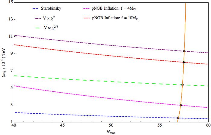
Figure 1: Numerical solution for the condition $H_{\rm infl}>m_{\varphi}$. The solid curve is a plot of $m_{\varphi}$ as a function of $N_{\rm max}$ as given by (3.2). The dashed curves are plots of the left hand side of (3.3) as a function of $N_{\rm max}$ for various models.

The condition is most stringent for the Starobinsky model, for which the right hand side and left hand side of (3.3) are equal for $m_{\varphi}\approx 1.5\times 10^{10}\phantom{s}\rm{TeV}$. We will be conservative and study the implications of the shift in the central value of $N_{k}$ if the mass of the modulus is at least two orders of magnitude below this i.e $m_{\varphi}<10^{8}\phantom{s}\rm{TeV}$ (this value will be used for all models).

As described in section 2.1, successful nucleosynthesis requires $m_{\varphi}>30\phantom{s}{\rm TeV}$. We will use this consideration to set the lower value of $m_{\varphi}$ in our analysis. In summary, we will use the range

$$10^{2}\phantom{s}{\rm TeV}<m_{\varphi}<10^{8}\phantom{s}{\rm TeV}$$ (3.4)

to study the effects of the epoch of modulus domination on inflationary predictions.

We now have all the ingredients necessary to compute the predictions for $n_{s}$ and $r$. For $m_{\varphi}$ in the range given by (3.4) the preferred range for $N_{k}$ is given by (2.7). On the other hand, if the mass of the modulus is greater than Hubble during inflation, the preferred range is 50-60. We compute the predictions for $n_{s}$ and $r$ for $m_{\varphi}=10^{3},10^{6}\phantom{s}\rm{and}\phantom{s}10^{8}\phantom{s}\rm{TeV}$.

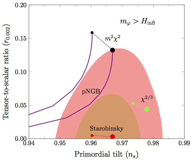
(a)

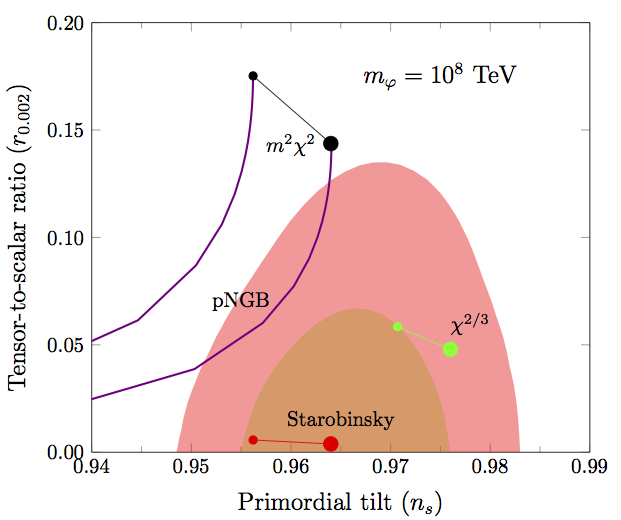
(b)

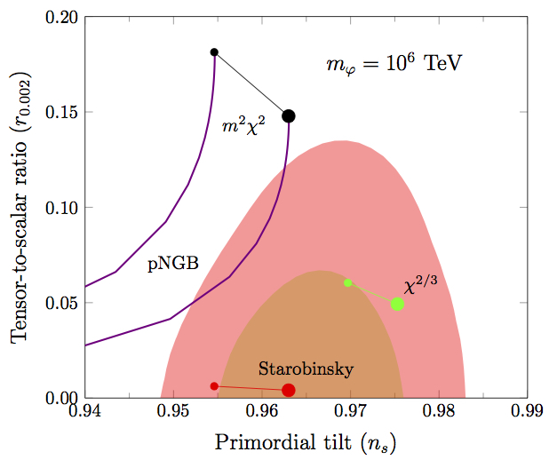
(c)

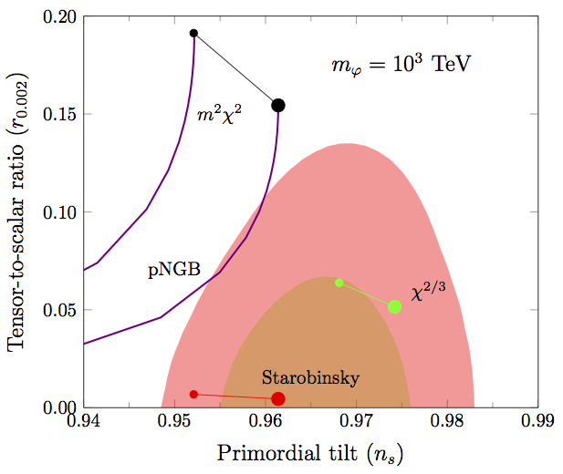
(d)

Figure 2: Inflationary predictions for $m^{2}\chi^{2}$ (black), Natural/pNGB inflation (purple), Axion monodromy (green), Starobinsky model (red). For the cases of no misalignment $(m_{\varphi}>H_{\rm infl})$, $m_{\varphi}=10^{3},10^{6},10^{8}\quad\rm{TeV.}$

The results are shown in Figure 2, the plot for the standard cosmological timeline (which is equivalent to $m_{\varphi}>H_{\rm infl}$) is also included for reference. The shaded regions correspond to the $1\tiny{-}\sigma$ and $2\tiny{-}\sigma$ results for $n_{s}$ and $r$ from planck 2015 analysis for TT modes and low P [22]. We find that for the $m^{2}\chi^{2}$ model even a very heavy modulus of mass $10^{8}\phantom{s}\rm{TeV}$ implies predictions for $n_{s}$ and $r$ which are well outside the $2\tiny{-}\sigma$ region. The axion monodromy model moves inside the $1\tiny{-}\sigma$ region for $m_{\varphi}$ below $10^{5}\phantom{s}{\rm TeV}$. The Starobinsky model remains in the $1\tiny{-}\sigma$ region for almost the entire mass range.

Finally, we would like to mention a general implication. For gravity mediated models moduli masses are tied to the scale of supersymmetry breaking. Thus, for gravity mediated models our results correlate inflationary predictions with the scale of supersymmetry breaking. The effect is significant even for models with a high scale of supersymmetry breaking.

4 A Bound on Moduli Masses

The consistency condition (2.5) can be used to obtain a bound on moduli masses given a model of inflation by taking input from observations on the value of $n_{s}$ [11]. The approach can be considered complimentary to that of the previous section where we discussed inflationary predictions as a function of the mass of the late time decaying modulus. In this section, we analyse the bound for our representative models and update some of the discussion in [11] in light of the planck 2015 data release [22].

We begin by briefly reviewing the derivation of the bound. Combining the expression for $N_{\rm mod}$ (2.6) with the consistency condition (2.5) one finds

$$\!\frac{1}{3}\ln\!\!\left(\!\frac{\!\sqrt{16\pi}M_{\rm pl}Y^{2}\!}{m_{\varphi}}\!\right)\!\!+\!{1\over 4}(\!1\!-\!3w_{\rm re1}\!)N_{\rm re1}\!+\!{1\over 4}(1\!-\!3w_{\rm re2})N_{\rm re2}\!\approx\!55.43\!-\!N_{k}\!+\!\frac{1}{4}\ln r\!+\!{1\over 4}\ln\!\left(\!\frac{{\rho_{k}}}{\rho_{\rm end}}\!\right)\!.$$ (4.1)

Various numerical and analytic studies of reheating suggest strongly that the effective equation of state during reheating epochs is less that one third i.e. $w_{\rm re1},w_{\rm re2}<1/3$ (see for e.g. [27, 4] for a discussion). With this, the second and third term in the left hand side of (4.1) are positive definite and the equation can immediately be converted to a bound for the mass of the modulus

$$m_{\varphi}\gtrsim\sqrt{16\pi}M_{\rm pl}Y^{2}~{}e^{-3\left(55.43-N_{k}+{1\over 4}\ln\left({\rho_{\rm k}/\rho_{\rm end}}\right)+\frac{1}{4}\ln r\right)}.$$ (4.2)

The bound applies only if $m_{\varphi}$ is less than Hubble during inflation (as equation (2.5) was derived under this assumption). We have used $w_{\rm re1},w_{\rm re2}<1/3$, in arriving at the bound. In specific models, one can hope to compute the parameters $w_{\rm re1},w_{\rm re2},N_{\rm re1}$ and $N_{\rm re2}$. Equation (4.1) can then be regarded as relating the mass of the modulus to the inflationary sector. Note that the longer the duration of reheating higher the value of $m_{\varphi}$.

Given a model of inflation and observational input on the value of $n_{s}$, one can explicitly compute the quantities in the exponent in the right hand side of (4.2). Typically, $N_{k}$ is related to $n_{s}$ by a relation of the form

$$N_{k}={\beta\over{1-n_{s}}},$$

where $\beta$ depends on the model of inflation. This makes the bound highly sensitive to the value of $n_{s}$. The planck 2015 release [22] gives the central value of $n_{s}$ to be 0.9680; there is a shift in the positive direction in comparison with the 2013 value of $n_{s}=0.9603$ [4]. This implies an increase in $N_{k}$ for inflationary models and thereby a more stringent bound.

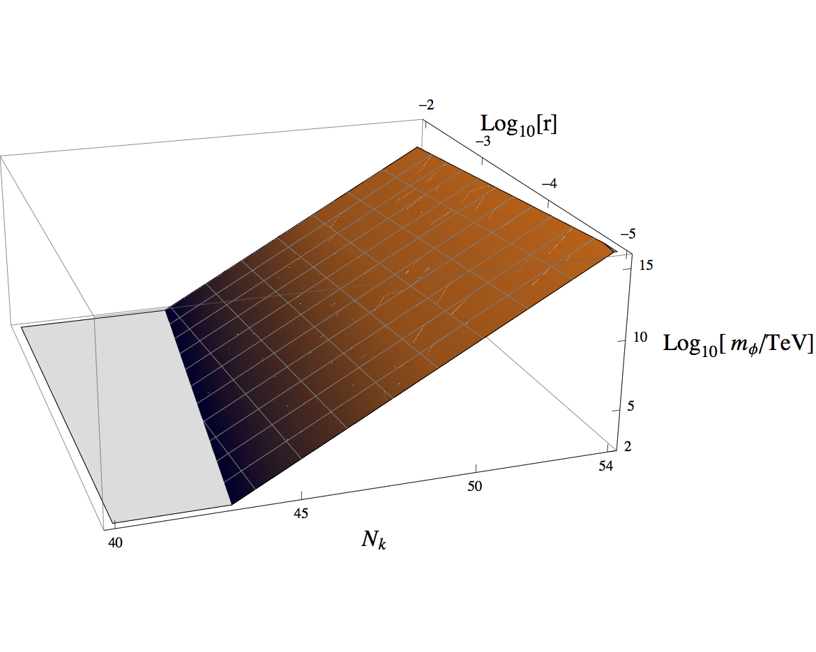
Figure 3: Bound on the modulus mass for small field models. The allowed values of $m_{\varphi}$ are in the region above the shaded plane. We have chosen $Y=1/10$.

Let us now discuss the bound in the context of our representative models. For polynomial potentials $V(\chi)\propto\chi^{\alpha}$, the bound simplifies to

$$m_{\varphi}\gtrsim\sqrt{16\pi}M_{\rm pl}Y^{2}e^{-3(55.85-\frac{(2+\alpha)}{2(1-n_{s})})}.$$ (4.3)

For the $m^{2}\chi^{2}$ model, the planck 2015 central value of $n_{s}$ gives the right hand side of (4.3) to be well above Hubble during inflation (as obtained in Figure 1); modular cosmology is incompatible with this value of $n_{s}$. The lower end of the $1\tiny{-}\sigma$ value gives $m_{\varphi}>10^{10}\phantom{s}\rm{TeV}$. On the other hand, for the axion monodromy model $(\alpha=2/3)$ (4.3) yields a value below the CMP bound (2.3), thus is not of phenomenological interest as a bound. The fact that the bound is not strong for the axion monodromy model is consistent with the results shown in figure 2 - the axion monodromy model is in the $1\tiny{-}\sigma$ region for $m_{\varphi}=10^{3}\phantom{s}\rm{TeV}$. Similarly, in the case of the Starobinsky model and pNGB inflation the value of the bound is in keeping with the results shown in figure 2.

For small field models, the second term in the exponent of the right hand side of (4.2) (the term involving the ratio of the energy densities at the time of horizon exit and end of inflation) makes a negligible contribution. Note that the functional form of the bound is such that it becomes stronger with decreasing $r$. In Figure 3 we show the allowed range for $m_{\varphi}$ as a function of $N_{k}$ and $r$. The plot illustrates that the scale for the bound is essentially set by $N_{k}$. For $N_{k}\gtrsim 50$ the bound is very strong; $m_{\varphi}\gtrsim 10^{7}\phantom{s}{\rm TeV}$. The bound is stronger than the CMP bound (2.3) as long as $N_{k}\gtrsim 44.5$. The plot in Figure 3 can be used to read off the implications of the bound for any small field model. It will be interesting to explore the implications of this bound for inflationary model building in moduli stabilised string compactifications.

5 Discussion and Conclusions

In this paper, we have studied the sensitivity of $n_{s}$ and $r$ to the mass of the lightest modulus in the context of modular cosmology. The results of section 3 clearly exhibit that it is important to explicitly incorporate the effect of the epoch of modulus domination in obtaining the preferred range of $N_{k}$. The effect can significantly alter the inflationary predictions for $n_{s}$ and $r$ of string/supergravity models; being relevant even for very heavy moduli $(m_{\varphi}\approx 10^{8}\phantom{s}\rm{TeV})$. Furthermore, future experiments [25] are likely to bring down the uncertainties in the measurement of $n_{s}$ by one order of magnitude; making our analysis all the more relevant. Given that modular cosmology is generic in string/supergravity models [5, 6, 7, 9, 10, 8] our results should have broad implications.

Our approach has been phenomenological; we have treated the mass of the lightest modulus as a free parameter and taken the initial displacement of the modulus (that results due to misalignment) to have a generic value. The results strongly motivate the study of specific models where the modulus mass takes a fixed value and it is possible to compute the value of the initial displacement explicitly. Some models worth exploring in this context are fibre inflation [24] and Kahler moduli inflation [26].

Another important direction in the study of specific models is first principles analysis of the reheating epoch. This can reduce the uncertainty in $N_{k}$, allowing for more precise predictions of $n_{s}$ and $r$. This question has received much attention recently [27, 28, 29]. The methods developed in [29] can be useful in analysing the decay of moduli particles.

More generally, modular cosmology can also have implications for dark matter, structure formation and the phenomenology of SUSY models [30]. It is natural to look for correlations between our results for CMB observables and other phenomenological signatures. Gravity mediated models are particularly interesting in this context, as the moduli masses are tied to the scale of supersymmetry breaking.

Appendix

A. Density Perturbations in Modular Cosmology

Our focus has been on models in which quantum fluctuations during the inflationary epoch are responsible for the density perturbations. Here we elaborate on this further in the context of modulus dominated cosmology. As discussed in section 2.1 the minimum of the potential of the late time decaying modulus depends on the inflaton expectation value; thus as the inflaton moves along its trajectory the expectation value of the late time decaying modulus (and potentially other moduli) necessarily changes. Thus, the trajectory in field space during inflation involves displacement along the inflaton direction, late time decaying modulus (and potentially other moduli). We will require the directions in field space orthogonal to the trajectory in field space during inflation to have mass of at least of the order of Hubble (this as we will see in what follows will ensure that isocurvature perturbations are suppressed). Infact, curvature couplings naturally lead to such mass terms of the order of Hubble (see for e.g.[15, 16]).

The perturbations generated are best understood in the formalism developed in [31] – coordinates in field space are chosen such that one of the coordinate directions is along the trajectory in field space (during the inflationary epoch) and the remaining are orthogonal to the trajectory in field space. The key result of [31] is that quantum fluctuations associated with the direction in field space parallel to the trajectory are adiabatic, while the ones orthogonal generate isocurvature perturbations. Thus, imposing the condition that the directions in field space orthogonal to the trajectory have mass at least of the order of Hubble ensures that isocurvature perturbations at the time of horizon exit are suppressed; the perturbations are to a very good approximation adiabatic at the time of horizon exit. We will denote the adiabatic perturbation at the time of horizon exit by $\cal{R}_{*}$ and the isocurvature perturbations by ${\cal{S}}^{i}_{*}$. These have to be evolved into the radiation epoch (after the decay of the modulus) to determine the strength of the temperature fluctuations they seed. The result of this evolution is given by a transfer matrix [32], which takes the general form (to keep the presentation simple we include one isocurvature direction, it is easily generalised to the case of multiple isocurvature perturbation directions)

$$\begin{bmatrix}\mathcal{R}_{\rm rad}\\ \mathcal{S}_{\rm rad}\end{bmatrix}=\begin{bmatrix}1&\mathcal{T}_{\rm RS}\\ 0&\mathcal{T}_{\rm SS}\end{bmatrix}\begin{bmatrix}\mathcal{R}_{*}\\ \mathcal{S}_{*}\end{bmatrix}$$

where $\mathcal{R}_{\rm rad}$ and $\mathcal{S}_{\rm rad}$ are the isocurvature and adiabatic perturbations after the modulus decay. An important feature of the transfer matrix is that the entries in the first column are completely model independent [32] - they follow from the fact that a purely adiabatic perturbation is conserved and does not lead to any isocurvature perturbations. On the other hand, the transfer functions $\mathcal{T}_{\rm RS}$ and $\mathcal{T}_{\rm SS}$ are model dependent. But, the form of the transfer matrix implies that if $\mathcal{S}_{*}<<\mathcal{R}_{*}$, then isocurvature perturbations remain suppressed and $\mathcal{R}_{\rm rad}$ is essentially determined by $\mathcal{R}_{*}$. Thus, for models in which the only light direction during the inflationary epoch is the trajectory in field space the density perturbations are adiabatic and determined by the curvature perturbation at the time of horizon exit.

Other scenarios to generate density perturbations are the curvaton scenario [33] and modulated fluctuations [34]. We shall not explore these possibilities here, see [35, 36] for their realisations in string models.

References

- [1] C. Burgess, M. Cicoli, and F. Quevedo arXiv:1306.3512 [hep-th]
- [2] E. Silverstein, arXiv:1311.2312 [hep-th]
- [3] D. Baumann and L. McAllister, arXiv:1404.2601 [hep-th].
- [4] P. A. R. Ade et al. [Planck Collaboration], arXiv:1303.5082 [astro-ph.CO].
- [5] G. D. Coughlan, W. Fischler, E. W. Kolb, S. Raby and G. G. Ross, Phys. Lett. B 131 (1983) 59;
- [6] T. Banks, D. B. Kaplan and A. E. Nelson, Phys. Rev. D 49 (1994) 779 [hep-ph/9308292];
- [7] B. de Carlos, J. A. Casas, F. Quevedo and E. Roulet, Phys. Lett. B 318 (1993) 447 [hep-ph/9308325].
- [8] F. Quevedo, Class. Quant. Grav. 19 (2002) 5721 [hep-th/0210292].
- [9] M. R. Douglas, arXiv:1204.6626 [hep-th].
- [10] B. S. Acharya, G. Kane and P. Kumar, Int. J. Mod. Phys. A 27 (2012) 1230012
- [11] K. Dutta and A. Maharana, Phys. Rev. D 91 (2015) 4, 043503 [arXiv:1409.7037 [hep-ph]].
- [12] A. R. Liddle and S. M. Leach, Phys. Rev. D 68 (2003) 103503 [astro-ph/0305263].
- [13] M. Dine, W. Fischler and D. Nemeschansky, Phys. Lett. B 136 (1984) 169.
- [14] G. D. Coughlan, R. Holman, P. Ramond and G. G. Ross, Phys. Lett. B 140 (1984) 44.
- [15] M. Dine, L. Randall and S. D. Thomas, Phys. Rev. Lett. 75 (1995) 398 [hep-ph/9503303].
- [16] M. Dine, L. Randall and S. D. Thomas, Nucl. Phys. B 458 (1996) 291 [hep-ph/9507453].
- [17] A. S. Goncharov, A. D. Linde and M. I. Vysotsky, Phys. Lett. B 147 (1984) 279.
- [18] A. D. Linde, Phys. Lett. B 129 (1983) 177.
- [19] L. McAllister, E. Silverstein and A. Westphal, Phys. Rev. D 82, 046003 (2010) [arXiv:0808.0706 [hep-th]]. E. Silverstein and A. Westphal, Phys. Rev. D 78, 106003 (2008) [arXiv:0803.3085 [hep-th]].
- [20] F. C. Adams, J. R. Bond, K. Freese, J. A. Frieman and A. V. Olinto, Phys. Rev. D 47 (1993) 426 [hep-ph/9207245].
- [21] A. A. Starobinsky, Phys. Lett. B 91 (1980) 99.
- [22] P. A. R. Ade et al. [Planck Collaboration], arXiv:1502.02114 [astro-ph.CO].
- [23] M. Kawasaki, K. Kohri and N. Sugiyama, Phys. Rev. Lett. 82, 4168 (1999) [astro-ph/9811437]. M. Kawasaki, K. Kohri and N. Sugiyama, Phys. Rev. D 62, 023506 (2000) [astro-ph/0002127].
- [24] M. Cicoli, C. P. Burgess and F. Quevedo, JCAP 0903 (2009) 013 [arXiv:0808.0691 [hep-th]].
- [25] L. Amendola et al. [Euclid Theory Working Group Collaboration], Living Rev. Rel. 16, 6 (2013) [arXiv:1206.1225 [astro-ph.CO]]. P. Andre et al. [PRISM Collaboration], arXiv:1306.2259 [astro-ph.CO]. A. Kosowsky, Physics 3, 103 (2010). E. S. Phinney et al., The Big Bang Observer: S. Kawamura, T. Nakamura, M. Ando, N. Seto, K. Tsubono, K. Numata, R. Takahashi and S. Nagano et al., Class. Quant. Grav. 23, S125 (2006).
- [26] J. P. Conlon and F. Quevedo, JHEP 0601 (2006) 146 [hep-th/0509012]. J. R. Bond, L. Kofman, S. Prokushkin and P. M. Vaudrevange, Phys. Rev. D 75 (2007) 123511 [hep-th/0612197]. A. Maharana, M. Rummel and Y. Sumitomo, arXiv:1504.07202 [hep-th].
- [27] L. Dai, M. Kamionkowski and J. Wang, Phys. Rev. Lett. 113 (2014) 041302 [arXiv:1404.6704 [astro-ph.CO]]. J. L. Cook, E. Dimastrogiovanni, D. A. Easson and L. M. Krauss, arXiv:1502.04673 [astro-ph.CO]. V. Domcke and J. Heisig, arXiv:1504.00345 [astro-ph.CO].
- [28] J. Ellis, M. A. G. Garcia, D. V. Nanopoulos and K. A. Olive, arXiv:1503.08867 [hep-ph].
- [29] J. Ellis, M. A. G. Garcia, D. V. Nanopoulos and K. A. Olive, arXiv:1505.06986 [hep-ph].
- [30] G. Kane, K. Sinha and S. Watson, arXiv:1502.07746 [hep-th]. T. Moroi and L. Randall, Nucl. Phys. B 570 (2000) 455 [hep-ph/9906527]. B. S. Acharya, P. Kumar, K. Bobkov, G. Kane, J. Shao and S. Watson, JHEP 0806 (2008) 064 [arXiv:0804.0863 [hep-ph]]. B. S. Acharya, G. Kane and E. Kuflik, arXiv:1006.3272 [hep-ph]. J. P. Conlon, S. S. Abdussalam, F. Quevedo and K. Suruliz, JHEP 0701 (2007) 032 [hep-th/0610129]; R. Blumenhagen, J. P. Conlon, S. Krippendorf, S. Moster and F. Quevedo, JHEP 0909 (2009) 007 [arXiv:0906.3297 [hep-th]]. L. Aparicio, M. Cicoli, S. Krippendorf, A. Maharana, F. Muia and F. Quevedo, arXiv:1409.1931 [hep-th]. L. Aparicio, M. Cicoli, B. Dutta, S. Krippendorf, A. Maharana, F. Muia and F. Quevedo, JHEP 1505 (2015) 098 [arXiv:1502.05672 [hep-ph]]. M. Cicoli, J. P. Conlon and F. Quevedo, Phys. Rev. D 87 (2013) 043520 [arXiv:1208.3562 [hep-ph]]. T. Higaki and F. Takahashi, JHEP 1211 (2012) 125 [arXiv:1208.3563 [hep-ph]]. R. Allahverdi, M. Cicoli, B. Dutta and K. Sinha, Phys. Rev. D 88, no. 9, 095015 (2013) [arXiv:1307.5086 [hep-ph]]. R. Allahverdi, B. Dutta and K. Sinha, Phys. Rev. D 82, 035004 (2010) [arXiv:1005.2804 [hep-ph]]. R. Allahverdi, B. Dutta and K. Sinha, Phys. Rev. D 87, 075024 (2013) [arXiv:1212.6948 [hep-ph]]. J. Fan, O. zsoy and S. Watson, Phys. Rev. D 90, 043536 (2014) [arXiv:1405.7373 [hep-ph]]. L. Iliesiu, D. J. E. Marsh, K. Moodley and S. Watson, Phys. Rev. D 89, 103513 (2014) [arXiv:1312.3636 [astro-ph.CO]]. R. Easther, R. Galvez, O. Ozsoy and S. Watson, Phys. Rev. D 89, 023522 (2014) [arXiv:1307.2453 [hep-ph]].
- [31] C. Gordon, D. Wands, B. A. Bassett and R. Maartens, Phys. Rev. D 63 (2001) 023506 [astro-ph/0009131].
- [32] L. Amendola, C. Gordon, D. Wands and M. Sasaki, Phys. Rev. Lett. 88 (2002) 211302 [astro-ph/0107089].
- [33] D. H. Lyth and D. Wands, Phys. Lett. B 524 (2002) 5 [hep-ph/0110002]; T. Moroi and T. Takahashi, Phys. Lett. B 522 (2001) 215 [Erratum-ibid. B 539 (2002) 303] [hep-ph/0110096]. K. Enqvist and M. S. Sloth, Nucl. Phys. B 626 (2002) 395 [hep-ph/0109214].
- [34] G. Dvali, A. Gruzinov and M. Zaldarriaga, density perturbations from inflation,” Phys. Rev. D 69 (2004) 023505 [astro-ph/0303591]. G. Dvali, A. Gruzinov and M. Zaldarriaga, inhomogeneous reheating, freezeout, and mass domination,” Phys. Rev. D 69 (2004) 083505 [astro-ph/0305548]. L. Kofman, astro-ph/0303614.
- [35] C. P. Burgess, M. Cicoli, M. Gomez-Reino, F. Quevedo, G. Tasinato and I. Zavala, JHEP 1008 (2010) 045 [arXiv:1005.4840 [hep-th]].
- [36] M. Cicoli, G. Tasinato, I. Zavala, C. P. Burgess and F. Quevedo, JCAP 1205 (2012) 039 [arXiv:1202.4580 [hep-th]].