Dirichlet eigenfunctions on the cube, sharpening the Courant nodal inequality

1. Introduction and Main result

Consider the Dirichlet eigenvalues of the Laplacian in the domain $\Omega$

(1) $$\left\{\begin{array}[]{rll}-\Delta u&=\lambda u&\text{ in }\Omega\\ u&=0&\text{ on }\partial\Omega.\end{array}\right.$$

We denote by $\{\lambda_{k}\}_{k\geq 1}=\{\lambda_{k}(\Omega)\}_{k\geq 1}$ the sequence of eigenvalues:

$$\lambda_{1}<\lambda_{2}\leq\lambda_{3}\leq...\leq\lambda_{k}\leq...$$

It is well known that the first eigenvalue is simple and the eigenfunction $u_{1}$ has a constant sign in $\Omega$. All the higher order eigenfunctions must change sign inside $\Omega$ and, consequently, must vanish inside $\Omega$.

We call nodal set of an eigenfunction $u_{k}$ associated with $\lambda_{k}$ the closure of the zero set of $u_{k}$,

$$\mathcal{N}(u_{k})=\overline{\{x\in\Omega;\ u_{k}(x)=0\}}.$$

This nodal set cuts the domain $\Omega\setminus\mathcal{N}(u_{k})$ into $\mu_{k}=\mu(u_{k})$ connected components called “nodal domains”.

The famous Courant nodal theorem [6] of 1923 states that

$$\mu(u_{k})\leq k.$$

We will say that an eigenvalue $\lambda$ is Courant sharp if $\lambda=\lambda_{k}$ and if there exists an associate eigenfunction with $k$ nodal domains. If it is always true in the case of dimension $1$ by the Sturm-Liouvillle theory, Pleijel’s theorem [24] asserts in 1956 that equality can only occur for a finite set of $k$’s, when the dimension is at least two.

Since we know that the first eigenfunction does not vanish and that the second eigenfunction has exactly two nodal domains, $\lambda_{1}$ and $\lambda_{2}$ are Courant sharp ($\mu_{1}=1$ and $\mu_{2}=2$). We are now interested in checking if other eigenvalues are Courant sharp.

Many papers (and some of them quite recent) have investigated in which cases this inequality is sharp: Pleijel [24], Helffer–Hoffmann-Ostenhof–Terracini [12, 13], Helffer–Hoffmann-Ostenhof [10, 11], Bérard-Helffer [2, 3, 4], Helffer–Persson-Sundqvist [15], Léna [19], Leydold [20, 21, 22]. All these results were devoted to $(2D)$-cases in open sets in $\mathbb{R}^{2}$ or in surfaces like $\mathbb{S}^{2}$ or $\mathbb{T}^{2}$.

The aim of the current paper is to look for analogous results for domains in $\mathbb{R}^{3}$ and, as $\AA.$Pleijel was suggesting (see below for an historical discussion), for the simplest case of the cube. More precisely, we will prove:

Theorem 1.1.

In the case of the cube $(0,\pi)^{3}$ the only eigenvalues of the Dirichlet Laplacian which are Courant sharp are the two first eigenvalues: $\lambda_{1}=3$ and $\lambda_{2}=6$.

2. Coming back to Pleijel’s paper

Outside the proof of Pleijel’s theorem in $2D$, Pleijel [24] (see also [2] for a more detailed analysis) considers as an example the case of the square which reads

Theorem 2.1.

In the case of the square the only eigenvalues which are Courant sharp for the Dirichlet Laplacian are the two first eigenvalues and the fourth one.

The proof was based on a first reduction to the analysis of the eigenvalues less than $68$ (the argument will be extended to the $(3D)$-case below and this is a quantitative version of the proof of Pleijel’s theorem), then all the other eigenvalues were eliminated using this time a more direct consequence of Faber-Krahn’s inequality, except three remaining cases for which Pleijel was rather sketchy which have to be treated by hand.

At the end of his celebrated paper $\AA$. Pleijel wrote:
” In order to treat, for instance the case of the free three-dimensional membrane $[0,\pi]^{3}$, it would be necessary to use, in a special case, the theorem quoted in [7], p. 394. This theorem which generalizes part of the Liouville-Rayleigh theorem for the string asserts that a linear combination, with constant coefficients, of the $n$ first eigenfunctions can have at most $n$ nodal domains. However, as far as I have been able to find there is no proof of this assertion in the literature.”
$\AA$. Pleijel was indeed speaking of a result presented in [7] as being proved in the thesis defended in 1932 at the University of Göttingen by Horst Herrmann (with R. Courant as advisor). This result was never published or confirmed and is now called the Courant-Herrmann conjecture [9]. Actually, it is said in [9] that the authors can not find any mention of the result in the thesis itself. This Courant-Herrmann conjecture was asserting that, for a given $k\in\mathbb{N}$, Courant’s theorem holds also for linear combinations of eigenfunctions associated with eigenvalues $\lambda_{j}$ with $j\leq k$.
Pleijel is not explicitly saying why he was needing this result but one could think that he is interested, because he speaks about the ”free problem” (i.e. the Neumann problem), in counting the number of components of the restriction of an eigenfunction to a face of the cube $(0,\pi)^{3}$. Looking for example to the zeroset of

$$(x,y,z)\mapsto a\cos x\cos y\cos nz+b\cos y\cos z\cos nx+c\cos z\cos x\cos ny\,,$$

one gets for fixed $z=0$, a linear combination of the eigenfunctions of the square $\cos x\cos y$, $\cos y\cos nx$ and $\cos x\cos ny$ corresponding to two different eigenspaces for the Neumann Laplacian in the square $(0,\pi)\times(0,\pi)$. We will not go further in this paper on the Neumann problem but similar questions could also occur in the Dirichlet problem and we typically meet below the eigenfunction

$$(x,y,z)\mapsto a\sin x\sin y\sin nz+b\sin y\sin z\sin nx+c\sin z\sin x\sin ny\,,$$

and will be interested for example in the intersection of its zero set with the hyperplace $\{z=\frac{\pi}{2}\}$ inside the cube (in the case $n=3$).

3. Reminder on Pleijel’s theorem in $3D$

Let us first prove that there are only a finite number of eigenvalues that satisfy $\mu_{k}:=\mu(u_{k})=k$. This proof was given in dimension $n$ by Bérard-Meyer [5].

Proposition 3.1.

If $\lambda_{k}$ is an eigenvalue of (1) such that $\lambda_{k-1}<\lambda_{k}$, and $u_{k}$ is an associated eigenfunction then:

(2) $$\lambda_{k}^{\frac{3}{2}}|\Omega|\geq\mu(u_{k})\frac{4}{3}\pi^{4}\,.$$

Proof.

Assume that the nodal set cuts the domain $\Omega$ in $\mu_{k}$ connected components and let us denote them by $\Omega_{i},1\leq i\leq\mu_{k}.$ Since $u_{k}$ does not vanish inside $\Omega_{i}$, it is equal to its first eigenvalue and now using the $(3D)$-Faber-Krahn inequality on each component (see for example Bérard-Meyer [5]):

$$\lambda_{k}^{\frac{3}{2}}|\Omega_{i}|\geq\frac{4}{3}\pi^{4}\,\text{ for }1\leq i\leq\mu_{k}\,.$$

Adding together all the equations we get (2). ∎

Theorem 3.2.

(3) $$\lim\sup_{k\rightarrow+\infty}\frac{\mu_{k}}{k}\leq\frac{9}{2\pi^{2}}<1\,.$$

In particular, there exists only a finite number of eigenvalues satisfying $\mu_{k}=k$.

Proof.

We start from the Weyl’s asymptotics for the counting function

(4) $$N(\lambda):=\#\{k\,,\,\lambda_{k}<\lambda\},$$

which reads

(5) $$N(\lambda)\sim\frac{1}{6\pi^{2}}|\Omega|\lambda^{\frac{3}{2}}\,.$$

For an eigenvalue $\lambda_{k}$ such that $\lambda_{k-1}<\lambda_{k}$, we have $N(\lambda_{k})=k-1\,.$ Then from

$$\lambda_{k}^{\frac{3}{2}}\sim\frac{6\pi^{2}}{|\Omega|}k$$

together with (2), we get (3). ∎

Remark 3.3.

It is clear from (3) that we cannot have an infinite number of eigenvalues satisfying $\mu_{k}=k$.

4. The case of the cube

Let us consider the cube $(0,\pi)\times(0,\pi)\times(0,\pi)$ for which an orthogonal basis of eigenfunctions for the Dirichlet problem is given by:

$$\left\{\begin{array}[]{rl}u_{\ell,m,n}(x,y,z)&=\sin(\ell x)\cdot\sin(my)\cdot\sin(nz)\,,\\ \lambda_{\ell,m,n}&=\ell^{2}+m^{2}+n^{2}\,,\end{array}\right.$$

for $\ell,m,n\geq 1$.
Applying Proposition 3.1 for this domain, we get

Proposition 4.1.

If $u_{k}$ is an eigenfunction associated with $\lambda_{k}$ such that $u_{k}$ has $k$ nodal domains and if $\lambda_{k-1}<\lambda_{k}$ we have:

(6) $$\frac{{\lambda_{k}}^{\frac{3}{2}}}{k}\geq\frac{4}{3}\pi\,.$$

Here we will try to find a lower bound for the number $N(\lambda)$, since we know the $\lambda$’s are equal to $\ell^{2}+m^{2}+n^{2}$ where $\ell,m,n$ are integers, so we need to count the number of the lattice points of $\mathbb{R}^{3}$ inside the sphere of radius $\sqrt{\lambda}$.

Lemma 4.2.

If $\lambda\geq 3$, then

(7) $$N(\lambda)>\frac{\pi}{6}\lambda^{\frac{3}{2}}-\frac{3\pi}{4}\lambda+3\sqrt{\lambda-2}-1\,.$$

The proof is given in the appendix.

Lemma 4.3.

If $u_{k}$ is an eigenfunction associated with $\lambda_{k}$ such that $u_{k}$ has $k$ nodal domains we have:

(8) $$\left(\frac{3}{4\pi}-\frac{\pi}{6}\right)\lambda^{\frac{3}{2}}+\frac{3\pi}{4}\lambda-3\sqrt{\lambda}+3>0\,.$$

Proof.

First by Courant theorem, we have necessarily $\lambda_{k-1}<\lambda_{k}\,$.
Applying (7), we have

$$k-1=N(\lambda)>\frac{\pi}{6}\lambda^{\frac{3}{2}}-\frac{3\pi}{4}\lambda+3\sqrt{\lambda-2}-1\,.$$

i.e.

(9) $$k>\frac{\pi}{6}\lambda^{\frac{3}{2}}-\frac{3\pi}{4}\lambda+3\sqrt{\lambda-2}\,.$$

Together with (6), this implies:

$$\left(\frac{3}{4\pi}-\frac{\pi}{6}\right)\lambda^{\frac{3}{2}}+\frac{3\pi}{4}\lambda>3\sqrt{\lambda-2}\,.$$

One immediately sees that, for $\lambda\geq 3\,$,

$$\sqrt{\lambda-2}-\sqrt{\lambda}=-\frac{2}{\sqrt{\lambda}+\sqrt{\lambda-2}}\geq-\frac{2}{1+\sqrt{3}}>-1\,.$$

∎

Now setting $\mu=\sqrt{\lambda}$ we get the third order inequation:

$$\left(\frac{3}{4\pi}-\frac{\pi}{6}\right)\mu^{3}+\frac{3\pi}{4}\mu^{2}-3\mu+3>0\,.$$

Using a calculator we can see that the only real root of the equation $\left(\frac{3}{4\pi}-\frac{\pi}{6}\right)\mu^{3}+\frac{3\pi}{4}\mu^{2}-3\mu+3=0$ is $\mu=6.97836\,$. This gives that the inequality is true only $0<\mu<6.97836\,,$ hence for $\lambda<48.7\,.$ So we have finally proved:

Proposition 4.4.

If $u_{k}$ is an eigenfunction associated with $\lambda_{k}$ such that $u_{k}$ has $k$ nodal domains and if $\lambda_{k-1}<\lambda_{k}$ , we have:

(10) $$\lambda_{k}\leq 48\,.$$

5. The list

In this section, we establish the list of the eigenvalues which are less than $48$ and determine which of these eigenvalues satisfy the necessary condition (6) for being Courant sharp.

k	$(\ell,m,n)$	$\lambda_{k}$
$\lambda_{1}$	(1,1,1)	3
$\lambda_{2}=\lambda_{3}=\lambda_{4}$	(1,1,2)	6
$\lambda_{5}=\lambda_{6}=\lambda_{7}$	$(1,2,2)$	9
$\lambda_{8}=\lambda_{9}=\lambda_{10}$	(1,1,3)	11
$\lambda_{11}$	(2,2,2)	12
$\lambda_{12}=\lambda_{13}=\lambda_{14}=\lambda_{15}=\lambda_{16}=\lambda_{17}$	(1,2,3)	14
$\lambda_{18}=\lambda_{19}=\lambda_{20}$	(2,2,3)	17
$\lambda_{21}=\lambda_{22}=\lambda_{23}$	(1,1,4)	18
$\lambda_{24}=\lambda_{25}=\lambda_{26}$	(1,3,3)	19
$\lambda_{27}=\lambda_{28}=\lambda_{29}=\lambda_{30}=\lambda_{31}=\lambda_{32}$	(1,2,4)	21
$\lambda_{33}=\lambda_{34}=\lambda_{35}$	(2,3,3)	22
$\lambda_{36}=\lambda_{37}=\lambda_{38}$	$(2,2,4)$	24
$\lambda_{39}=\lambda_{40}=\lambda_{41}=\lambda_{42}=\lambda_{43}=\lambda_{44}$	$(1,3,4)$	26
$\lambda_{45}=\lambda_{46}=\lambda_{47}=\lambda_{48}$	$(3,3,3)\ \&\ (1,1,5)$	27
$\lambda_{49}=\lambda_{50}=\lambda_{51}=\lambda_{52}=\lambda_{53}=\lambda_{54}$	$(2,3,4)$	29
$\lambda_{55}=\lambda_{56}=\lambda_{57}=\lambda_{58}=\lambda_{59}=\lambda_{60}$	$(1,2,5)$	30
$\lambda_{61}=\lambda_{62}=\lambda_{63}=\lambda_{64}=\lambda_{65}=\lambda_{66}$	$(1,4,4)\ \&\ (2,2,5)$	33
$\lambda_{67}=\lambda_{68}=\lambda_{69}$	$(3,3,4)$	34
$\lambda_{70}=\lambda_{71}=\lambda_{72}=\lambda_{73}=\lambda_{74}=\lambda_{75}$	$(1,3,5)$	35
$\lambda_{76}=\lambda_{77}=\lambda_{78}$	$(2,4,4)$	36
$\lambda_{79}=\lambda_{80}=\lambda_{81}=\lambda_{82}=\lambda_{83}=\lambda_{84}=\lambda_{85}=\lambda_{86}=\lambda_{87}$	$(1,1,6)\ \&\ (2,3,5)$	38
$\lambda_{88}=\lambda_{89}=\lambda_{90}=\lambda_{91}=\lambda_{92}=\lambda_{93}=\lambda_{94}=\lambda_{95}=\lambda_{96}$	$(1,2,6)\ \&\ (3,4,4)$	41
$\lambda_{97}=\lambda_{98}=\lambda_{99}=\lambda_{100}=\lambda_{101}=\lambda_{102}$	$(1,4,5)$	42
$\lambda_{103}=\lambda_{104}=\lambda_{105}$	$(3,3,5)$	43
$\lambda_{106}=\lambda_{107}=\lambda_{108}$	$(2,2,6)$	44
$\lambda_{109}=\lambda_{110}=\lambda_{111}=\lambda_{112}=\lambda_{113}=\lambda_{114}$	$(2,4,5)$	45
$\lambda_{115}=\lambda_{116}=\lambda_{117}=\lambda_{118}=\lambda_{119}=\lambda_{120}$	$(1,3,6)$	46
$\lambda_{121}$	$(4,4,4)$	48

Coming back to the consequences of Faber-Krahn’s inequality, one can check that among all the values on the table, the only eigenvalues that satisfy inequality (6) and $\lambda_{k-1}<\lambda_{k}$ are $\lambda_{1}\,$, $\lambda_{2}\,$, $\lambda_{5}\,$, $\lambda_{8}\,$ and $\lambda_{12}\,$.

Proposition 5.1.

The only eigenvalues which can be ”Courant sharp” are the eigenvalues $\lambda_{k}$ with $k=1,2,5,8$ and $12$.

As $\lambda_{1}$ and $\lambda_{2}$ are Courant sharp, the only remaining cases to analyze correspond to $k=5,8,12$.

In the next section we will by a finer analysis involving symmetries eliminate other cases.

6. Courant theorem with symmetry

We first recall some generalities which come back to Leydold [20], and were used in various contexts [21, 22, 15, 13]. Suppose that there exists an isometry $g$ such that $g(\Omega)=\Omega$ and $g^{2}={\sf Id}\,$. Then $g$ acts naturally on $L^{2}(\Omega)$ by $gu({\bf x})=u(g^{-1}{\bf x})\,,\,\forall{\bf x}\in\Omega\,,$ and one can naturally define an orthogonal decomposition of $L^{2}(\Omega)$

$$L^{2}(\Omega)=L^{2}_{\sf odd}\oplus L^{2}_{\sf even}\,,$$

where by definition $L^{2}_{\sf odd}=\{u\in L^{2}\,,\,gu=-u\}$, resp. $L^{2}_{\sf even}=\{u\in L^{2}\,,\,gu=u\}$. These two spaces are left invariant by the Laplacian and one can consider separately the spectrum of the two restrictions. Let us explain for the “odd case” what could be a Courant theorem with symmetry. If $u$ is an eigenfunction in $L^{2}_{\sf odd}$ associated with $\lambda$, we see immediately that the nodal domains appear by pairs (exchanged by $g$) and following the proof of the standard Courant theorem we see that if $\lambda=\lambda^{\sf odd}_{j}$ for some $j$ (that is the $j$-th eigenvalue in the odd space), then the number $\mu(u)$ of nodal domains of $u$ satisfies $\mu(u)\leq j$.
We get a similar result for the ”even” case (but in this case a nodal domain $D$ is either $g$-invariant or $g(D)$ is a distinct nodal domain).
These remarks may lead to improvements when each eigenspace has a specific symmetry. As we shall see, this will be the case for the cube with the map $(x,y,z)\mapsto(\pi-x,\pi-y,\pi-z)$.
We observe indeed that

$$u_{\ell,m,n}(\pi-x,\pi-y,\pi-z)=(-1)^{\ell+m+n+1}u_{\ell,m,n}(x,y)\,,$$

and that

$$\ell^{2}+m^{2}+n^{2}\equiv\ell+m+n\,({\rm mod}.2)\,.$$

Hence, for a given eigenvalue the whole eigenspace is even if $\ell+m+n$ is odd and odd if $\ell+m+n$ is even. Equivalently, the whole eigenspace is even if the eigenvalue is odd and even if the eigenvalue is odd.

Application.
$\lambda_{5}$ is not Courant sharp. The eigenspace associated with $\lambda_{5}=9$ is even. This is the second one (in this even space). Hence it should have less than four nodal domains by Courant’s theorem with symmetry and has labelling $5$.

$\lambda_{12}$ is not Courant sharp.

$\lambda_{12}=14$ is the fifth eigenvalue in the odd space with respect to $\sigma$. It should has less than $10$ nodal domains and has labelling $12$.

7. The remaining value: $k=8$

7.1. Main result

The proof of our main theorem relies now on the analysis of the last case which is the object of the next proposition.

Proposition 7.1.

In the eigenspace associated with $\lambda_{8}$ the eigenfunctions have either $2$, $3$ or $4$ nodal domains. In particular $\lambda_{8}$ cannot be Courant sharp.

7.2. Preliminaries

For the value $\lambda_{8}=11$ we have to analyze the zeroset of

$$\Phi_{a,b,c}(x,y,z):=a\sin x\sin y\sin 3z+b\sin y\sin z\sin 3x+c\sin z\sin x\sin 3y\,,$$

for $(a,b,c)\neq(0,0,0)$ .

This looks nice because we can divide by $\sin x\sin y\sin z$ and by making the change of coordinates $u=\cos x$, $v=\cos y$, $w=\cos z$, we get for the zero set of $\Phi_{a,b,c}$ in the new coordinates a quadric surface $\mathcal{Q}_{a,b,c}$ to analyze in the cube $\mathcal{C}=(-1,1)^{3}\,$, whose equation is

$$(\mathcal{Q}_{a,b,c})\quad 4\,(au^{2}+bv^{2}+cw^{2})-(a+b+c)=0\,,$$

for $(a,b,c)\neq(0,0,0)$ .

When $a+b+c\neq 0$, we immediately see that there are no critical points inside the cube, so the nodal set is simply an hypersurface (cylinder, ellipsoid or hyperboloid with one or two sheets). In this case, this is the analysis at the six faces of the cube which will be decisive for analyzing possible changes in the number of connected components. In the case when $a+b+c=0$, we have a double cone with a unique critical point at $(0,0,0)$.
In the next subsections, we discuss the different cases.

7.3. Cylinder

This corresponds to the case $abc=0\,$. We can use the (2D)- analysis as done in [2]. It is known that the number of nodal domains can only be 2,3 or 4 (See Section 3.1 and figure 2.1 there). See figure 1.

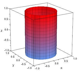
(a)  
$(a,b,c)=(1,1,0)$

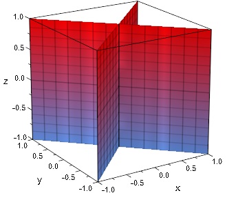
(b)  
$(a,b,c)=(1,-1,0)$

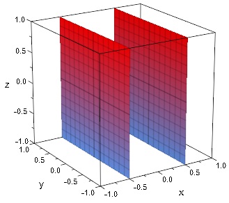
(c)  
$(a,b,c)=(1,0,0)$

Figure 1. Cylinders

7.4. Double cone

This corresponds to $abc\neq 0$ and $a+b+c=0\,$. The equation of $\mathcal{Q}_{a,b,c}$ is:

$$au^{2}+bv^{2}=-cw^{2}\,.$$

One can verify that the intersection of this cone with each horizontal side $w=\pm 1$ is exactly at the vertices of the cube $u^{2}=v^{2}=1$, and that the intersection with each vertical face is a hyperbola. Therefore there are three connected components of $\mathcal{C}\setminus\mathcal{Q}_{a,b,c}$. See figure 2.

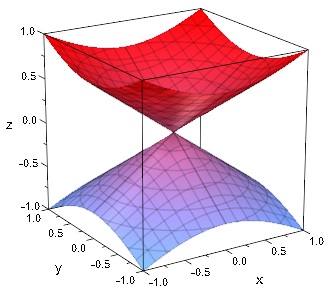
Figure 2. Double cones. $(a,b,c)=(0.2,0.2,-0.4)$

7.5. Ellipsoid

This corresponds to $abc\neq 0$, with a, b, c of the same sign. Without loss of generality, we can assume that $0<a\leq b\leq c$ and that $a+b+c=1$. We note that this implies $\frac{3}{2}(a+b)\leq a+2b\leq 1$.

(11) $$au^{2}+bv^{2}+(1-a-b)w^{2}=\frac{1}{4}\,.$$

We denote by $\Omega_{a,b,c}$ the open full ellipsoid delimited by $\mathcal{Q}_{a,b,c}$.
Let us look at the intersection of $\mathcal{Q}_{a,b,c}$ with the horizontal faces. We have

$$au^{2}+bv^{2}\leq-\frac{3}{4}+\frac{2}{3}<0\,.$$

We deduce that in this case there are no possible intersections with the horizontal faces, and therefore two subcases can occur depending on the intersection of $\mathcal{Q}_{a,b,c}$ with the vertical edges. This set is determined by

(12) $$(1-a-b)w^{2}=\frac{1}{4}-(a+b)\,,\,w\in(-1,+1)\,.$$

See figure 3.
Subcase $(a+b)>\frac{1}{4}\,$.
The ellipsoid $\mathcal{Q}_{a,b,c}$ does not touch the vertical edges and in this case $\mathcal{C}\cap\overline{\Omega_{a,b,c}}^{\,c}$ is connected and $\mathcal{C}\setminus\mathcal{Q}_{a,b,c}$ has exactly two connected components.
Subcase $(a+b)\leq\frac{1}{4}\,.$
$\mathcal{Q}_{a,b,c}$ cuts each vertical edge along a segment $[-w_{0},+w_{0}]$ with $w_{0}=\sqrt{\left(\frac{1}{4}-(a+b)\right)/(1-a-b)}$. The intersection of $\mathcal{Q}_{a,b,c}$ with each vertical face of the cube is the union of two arcs of an ellipse. In this case it is clear that $\mathcal{C}\setminus\mathcal{Q}_{a,b,c}$ has three connected components.

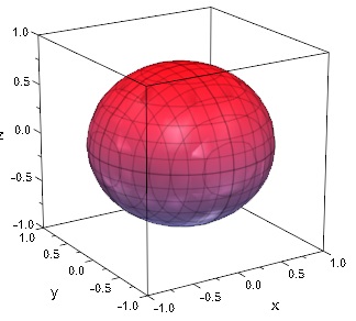
(a) $(a,b,c)\\ =(0.3,0.3,0.4)$

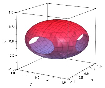
(b) $(a,b,c)\\ =(0.2,0.2,0.6)$

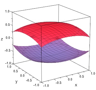
(c) $(a,b,c)\\ =(0.1,0.1,0.8)$

Figure 3. Ellipsoids

7.6. One sheet hyperboloid

This corresponds to $abc\neq 0$, a,b,c not of the same sign and $(abc)(a+b+c)<0\,$. Without loss of generality, we can assume that $b\geq a>0$, $c<0$ and $a+b+c=1\,$. We note that this implies that $\mathcal{Q}_{a,b,c}\cap\{w=0\}$ is an ellipse contained in the cube.

The equation of $\mathcal{Q}_{a,b,c}$ can be written as:

$$au^{2}+bv^{2}=\frac{1}{4}-cw^{2}\,.$$

$\mathcal{Q}_{a,b,c}$ cuts $\mathbb{R}^{3}$ into two components $\Omega_{a,b,c}^{+}$ and $\Omega_{a,b,c}^{-}$ where $\Omega_{a,b,c}^{+}$ contains $(0,0,0)$. But we have to look inside the cube.

We first observe that $\mathcal{Q}_{a,b,c}$ has empty intersection the vertical edges. We have indeed

$$a+b=1-c>\frac{1}{4}-c\geq\frac{1}{4}-cw^{2}\,.$$

We now look at the intersection with $w=0$. We get an ellipse $\mathcal{E}^{0}_{a,b,c}:=\mathcal{Q}_{a,b,c}\cap\{w=0\}$, whose equation is

$$au^{2}+bv^{2}=\frac{1}{4}\,.$$

We observe that this ellipse could be included in the cube, if $a>\frac{1}{4}$ or not if $a\leq\frac{1}{4}$.

We also look at the intersection with the upper horizontal face. We note that the ellipse $\mathcal{E}^{1}_{a,b,c}:=\mathcal{Q}_{a,b,c}\cap\{w=1\}$ has always a non empty intersection with this face.

Four subcases appear (See figure 4):

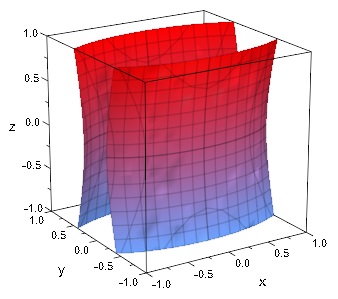
(a) $(a,b,c)\\ =(0.2,0.9,0.1)$

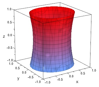
(b) $(a,b,c)\\ =(0.5,0.6,-0.1)$

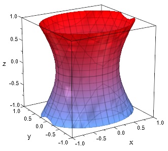
(c) $(a,b,c)\\ =(0.5,0.8,-0.3)$

(d) $(a,b,c)\\ =(0.8,0.8,-0.6)$

Figure 4. One Sheet Hyperboloid

Subcase $a\leq\frac{1}{4}$
Under this condition $\mathcal{Q}_{a,b,c}\cap\{v=0\}\cap\mathcal{C}$ is empty. Hence $\{v=0\}\cap\mathcal{C}$ is contained in one nodal domain which is invariant by $v\mapsto-v$. The other nodal domains are exchanged by this symmetry. This gives an odd number of nodal domains and this can not be Courant sharp because the labelling is $8$. More precisely the two curves in $\mathcal{C}$ defined by:

$$v=\pm\sqrt{\frac{\frac{1}{4}-au^{2}-cw^{2}}{b}}$$

cut the cube in three components.

The three last subcases are under the condition that $a>\frac{1}{4}$. We note that this condition implies that $\mathcal{E}^{0}_{a,b,c}$ is strictly included in the square $(-1,+1)\times(-1,+1)$ and the discussion continues according to the position of $\mathcal{E}^{1}_{a,b,c}$ in the horizontal face.

Subcase $\frac{1}{4}<a\leq b<\frac{3}{4}$
$\mathcal{E}^{1}_{a,b,c}$ is contained in the horizontal face and $\mathcal{Q}_{a,b,c}$ cuts the cube in two connected domains.

Subcase $\frac{1}{4}<a<\frac{3}{4}\leq b$
$\mathcal{E}^{1}_{a,b,c}\cap\partial\mathcal{C}$ consists of two curves but $\mathcal{Q}_{a,b,c}$ continue to cut the cube in two domains. For joining two points of $\Omega^{-}_{a,b,c}\cap\partial\mathcal{C}$ one can always go to a point in $\{w=0\}$ outside of $\mathcal{E}^{0}_{a,b,c}$ and use the connexity (inside the square $\mathcal{C}$ $\cap$ $\{w=0\}$) of the complementary of the full ellipse.

Subcase $\frac{3}{4}\leq a$
$\mathcal{E}^{1}_{a,b,c}\cap\mathcal{C}$ consists of four curves. $\mathcal{Q}_{a,b,c}$ continue to cut the cube in two domains.

7.7. Two sheets hyperboloid

This corresponds to $abc\neq 0$, a,b,c not of the same sign and $(abc)(a+b+c)>0$ .
We can assume $b\geq a>0$, $c<0$ and $a+b+c=-1\,.$ The equation of $\mathcal{Q}_{a,b,c}$ can be written as:

$$au^{2}+bv^{2}=-\frac{1}{4}-cw^{2}\,.$$

The hyperplane $\{w=0\}$ is contained in one connected component. Hence looking at the symmetry $w\mapsto-w$, we get that necessarily an odd number ($\geq 3$) of nodal domains and $\leq 8$ by Courant’s theorem. Hence we know that it cannot be Courant sharp.
More precisely, $\mathcal{Q}_{a,b,c}$ meets the hyperplane $\{w=1\}$ along the ellipse $\mathcal{E}_{a,b,c}$ which this time contains the horizontal upper face of the cube. The analysis of the intersection along each of the vertical faces (two symmetric curves by $w\mapsto-w$) shows that we always have exactly three connected components. See figure 5.

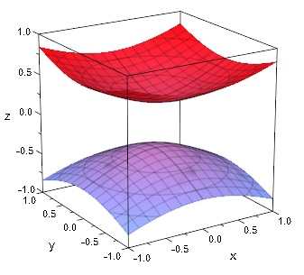
Figure 5. Two Sheets Hyperboloid. $(a,b,c)=(0.8,0.8,=-2.6)$

8. Conclusion

In this paper we have analyzed the problem in the simplest example proposed by $\AA$. Pleijel. One can of course ask for similar questions for other geometries starting with the parallelepipeds, the ball, the flat tori… The situation for $(0,\alpha\pi)\times([0,\beta\pi)\times(0,\gamma\pi)$ is in principle easier in the ”irrational” case when $\alpha\ell^{2}+\beta m^{2}+\gamma n^{2}=\alpha\ell_{1}^{2}+\beta m_{1}^{2}+\gamma_{1}n_{1}^{2}$ implies $(\ell,m,n)=(\ell_{1},m_{1},n_{1})$. Each eigenvalue $\alpha\ell^{2}+\beta m^{2}+\gamma n^{2}$ is indeed of multiplicity $1$ and the corresponding eigenfunction has $\ell mn$ nodal domains.
One can also think of analyzing ”thin structures” (for example $\gamma$ small or $\beta+\gamma$ small, where previous results in lower dimension can probably be used) in the spirit of [10] and get partial results. Another interesting question would be to analyze the Neumann problem for the cube in the spirit of [15].

Acknowledgements
The pictures were obtained by using the programme MATLAB. This paper was achieved when the two authors were invited at the Isaac Newton Institute for mathematical sciences in Cambridge. Moreover the first author was supported there as Simons foundation visiting fellow.

Appendix A The proof of Lemma 4.2

We follow an idea appearing in the $(2D)$ case in a course of R. Laugesen [18]. We start by assuming that $\lambda$ is not an eigenvalue. With each triple $(\ell,m,n)$ with $\ell\geq 1$, $m\geq 1$, $n\geq 1$, we associate the cube

$$Q_{\ell,m,n}=[\ell-1,\ell]\times[m-1,m]\times[n-1,n]\,.$$

We observe that

$$N(\lambda)=\sum_{\ell^{2}+m^{2}+n^{2}<\lambda,\ell\geq 1,m\geq 1,n\geq 1}A(Q_{\ell,m,n})\leq\frac{\pi}{6}\lambda^{\frac{3}{2}}\,.$$

We are interested in the lower bound. The claim of Laugesen is that

(13) $$N(\lambda)>A(B_{\lambda})\,,$$

where

$$B_{\lambda}:=\{(x+1)^{2}+(y+1)^{2}+(z+1)^{2}<\lambda,x>0,y>0,z>0\}.$$

The observation is that

$$B_{\lambda}\subset\cup_{\ell^{2}+m^{2}+n^{2}<\lambda,\ell\geq 1,m\geq 1,n\geq 1}Q_{\ell,m,n}\,.$$

For $t>0$, $[t]_{+}$ denotes the smallest integer $\geq t$.
Let $(x,y,z)\in B_{\lambda}$, then it is immediate to see that $(x,y)\in Q_{[x]_{+},[y]_{+},[z]_{+}}$. It remains to verify that

$$Q_{[x]_{+},[y]_{+},[z]_{+}}\subset D(0,\sqrt{\lambda})\,.$$

But we have, for $(x,y,z)\in B_{\lambda}$,

$$[x]_{+}^{2}+[y]_{+}^{2}+[z]_{+}^{2}\leq(x+1)^{2}+(y+1)^{2}+(z+1)^{2}<\lambda\,.$$

Coming back to (13), we have to find a lower bound for the area of $B_{\lambda}$. We note that by translation by the vector $(1,1,1)$:

(14) $$A(B_{\lambda})=A(C_{\lambda})\,,$$

where

$$C_{\lambda}:=D(0,\sqrt{\lambda})\cap\{x>1\}\cap\{y>1\}\cap\{z>1\}\,.$$

Let $\chi$ the characteristic function of the interval $(0,1)$. We have to compute the integral

$$A(C_{\lambda})=\int_{D(0,\sqrt{\lambda})}(1-\chi(x))(1-\chi(y))(1-\chi(z))dxdydz\,.$$

Developing the formula and using the symmetry by permutation of the variables, we get, if $\lambda\geq 3$,

(15) $$\begin{array}[]{ll}A(C_{\lambda})&=\quad\int_{D(0,\sqrt{\lambda})}dxdydz\\ &\quad-3\int_{D(0,\sqrt{\lambda})}\chi(x)dxdydz\\ &\quad+3\int_{D(0,\sqrt{\lambda})}\chi(x)\chi(y)dxdydz\\ &\quad-\int_{D(0,\sqrt{\lambda})}\chi(x)\chi(y)\chi(z)dxdydz\,.\end{array}$$

It is then immediate to get the lemma by observing that

(16) $$\int_{D(0,\sqrt{\lambda})}\chi(x)\chi(y))dxdydz>\sqrt{\lambda-2}\,.$$

We have assumed till now that $\lambda$ was not an eigenvalue. But if $\lambda$ is an eigenvalue $>3$, we can apply the previous result for an increasing sequence $\hat{\lambda}_{j}$ such that $\hat{\lambda}_{j}\rightarrow\lambda$ (where $\hat{\lambda}_{j}>3$ is not an eigenvalue). According to our definition of $N(\lambda)$ in (4), we can pass to the limit and observing that in (16) the inequality is uniformly strict when applied to the sequence $\lambda_{j}$ , we keep the strict inequality when passing to the limit. The case $\lambda=3$ can be verified directly.

References

- [1] P. Bérard. Inégalités isopérimétriques et applications. Domaines nodaux des fonctions propres. SEDP 1981-1982, École Polytechnique.
- [2] P. Bérard and B. Helffer. Dirichlet eigenfunctions of the square membrane: Courant’s property, and A. Stern’s and Å. Pleijel’s analyses. arXiv:14026054. To appear in the Springer Proceedings in Mathematics Statistics - PROMS (2015), MIMS-GGTM conference in memory of M.S. Baouendi. A. Baklouti, A. El Kacimi, S. Kallel, and N. Mir Editors.
- [3] P. Bérard, B. Helffer. A. Stern’s analysis of the nodal sets of some families of spherical harmonics revisited. Preprint July 2014. ArXiv: 1407.5564.
- [4] P. Bérard, B. Helffer. Courant sharp eigenvalues for the equilateral torus, and for the equilateral triangle. ArXiv: 1503.00117.
- [5] P. Bérard, D. Meyer. Inégalités isopérimétriques et applications. Annales Scientifiques de l’École Normale Supérieure, Sér. 4, 15 (3) (1982), 513–541.
- [6] R. Courant. Ein allgemeiner Satz zur Theorie der Eigenfunktionen selbstadjungierter Differentialausdrücke, Nachr. Ges. Göttingen (1923), 81–84.
- [7] R. Courant and D. Hilbert. Methods of Mathematical Physics, Vol. 1. New York (1953).
- [8] C. Faber. Beweis, daß unter allen homogenen Membrane von gleicher Fläche und gleicher Spannung die kreisförmige die tiefsten Grundton gibt. Sitzungsber. Bayer. Akad. Wiss., Math. Phys. Munich (1923), 169–172.
- [9] G.M.L. Gladwell and H. Zhu. The Courant-Herrmann conjecture. Z. Angew. Math.Mech. 83 (4) (2003), 275–281.
- [10] B. Helffer, T. Hoffmann-Ostenhof. Minimal partitions for anisotropic tori. J. Spectr. Theory 4(2) (2014), 221–233.
- [11] B. Helffer, T. Hoffmann-Ostenhof. A review on large k minimal spectral k-partitions and Pleijel’s Theorem. Proceedings of the congress in honour of J. Ralston (2013), in Contemporary Mathematics 640, Spectral Theory and Partial Differential Equations, G. Eskin, L. Friedlander, J. Garnett editors (2015), 39–58.
- [12] B. Helffer, T. Hoffmann-Ostenhof, S. Terracini. Nodal domains and spectral minimal partitions. Ann. Inst. H. Poincaré Anal. Non Linéaire 26 (2009), 101–138.
- [13] B. Helffer, T. Hoffmann-Ostenhof, S. Terracini. On spectral minimal partitions : the case of the sphere. Around the Research of Vladimir Maz’ya III, International Math. Series. 13 (2010), 153–179.
- [14] B. Helffer, T. Hoffmann-Ostenhof, S. Terracini. Nodal minimal partitions in dimension 3. DCDS-A, 28 (2) (2010), special issues Part I, dedicated to Professor Louis Nirenberg on the occasion of his 85th birthday.
- [15] B. Helffer and M. Persson-Sundqvist. Nodal domains in the square—the Neumann case. ArXiv:1410.6702. To appear in Moscow Mathematical Journal (2015).
- [16] H. Herrmann. Beziehungen zwischen den Eigenwerten und Eigenfunktionen verschiedener Eigenwertprobleme. Math. Z. 40 (1935), 221–241.
- [17] E. Krahn. Über eine von Rayleigh formulierte minimal Eigenschaft des Kreises. Math. Ann. 94 (1925), 97-100.
- [18] R.S. Laugesen. Spectral theory of Partial Differential Equations. University of Illinois at Urbana-Champaign (2011).
- [19] C. Léna. Courant-sharp eigenvalues of a two-dimensional torus. ArXiv:1501.02558.
- [20] J. Leydold. Knotenlinien und Knotengebiete von Eigenfunktionen. Diplom Arbeit, Universität Wien (1989), unpublished.
- [21] J. Leydold. On the number of nodal domains of spherical harmonics. PHD, Vienna University (1992).
- [22] J. Leydold. On the number of nodal domains of spherical harmonics. Topology 35 (1996), 301–321.
- [23] J. Peetre. A generalization of Courant nodal theorem. Math. Scandinavica 5 (1957), 15–20.
- [24] Å. Pleijel. Remarks on Courant’s nodal theorem. Comm. Pure. Appl. Math. 9 (1956), 543–550.
- [25] F. Pockels. Über die partielle Differentialgleichung and deren Auftreten in mathematischen Physik. Historical Math. Monographs. Cornell University (2013) (originally Teubner- Leipzig 1891).
- [26] I. Polterovich. Pleijel’s nodal domain theorem for free membranes. Proceeding of the AMS, Volume 137, Number 3, March 2009, 1021-1024.
- [27] A. Stern. Bemerkungen über asymptotisches Verhalten von Eigenwerten und Eigenfunktionen. Diss. Göttingen 1925.
- [28] J. Toth and S. Zelditch. Counting nodal lines that touched the boundary of an analytic domain. ArXiv: 0710.0101, 1-27.
- [29] H. Weyl. Über die asymptotische Verteilung der Eigenwerte. Nachrichten der Königlichen Gesellschaft der Wissenschaften zu Göttingen (1911), 110–117.