Determination of normalized electric eigenfields in microwave cavities with sharp edges

Abstract

The magnetic field integral equation for axially symmetric cavities with perfectly conducting piecewise smooth surfaces is discretized according to a high-order convergent Fourier–Nyström scheme. The resulting solver is used to accurately determine eigenwavenumbers and normalized electric eigenfields in the entire computational domain.

1 Introduction

This work is on a numerical solver for the time harmonic Maxwell equations in axially symmetric microwave cavities with piecewise smooth and perfectly electric conducting (PEC) surfaces. We use the interior magnetic field integral equation (MFIE) together with a charge integral equation (ChIE) and high-order convergent Fourier–Nyström discretization to find normalized electric eigenfields to high accuracy.

The intended primary application of our solver is in computational accelerator technology. Our experience is that our solver more than doubles the range of frequencies for which electric and magnetic eigenfields can be accurately evaluated, in comparison with finite element method programs commonly used. This opens up for improved evaluation of, so called, wakefields. Wakefields affect particle trajectories during accelerator operation and wakefield prediction is therefore of great importance in accelerator design, see [30, Chapter 11].

Our solver is based on the work [20], which in turn draws on progress in [3, 19, 28, 32]. A major step forward from [20] is the efficient treatment of piecewise smooth surfaces and field singularities at sharp edges. For this, we rely on a method called recursively compressed inverse preconditioning (RCIP) [21].

The RCIP method can be seen as an automated tool to enhance the performance of panel-based Nyström discretization schemes for Fredholm second kind integral equations in the presence of boundary singularities. For the determination of normalized eigenfields in microwave cavities with sharp edges, and from a numerical point of view, it is important to resolve boundary singularities and their associated non-smooth fields to high precision. This is so since these fields give non-negligible contributions to electric and magnetic energies needed in the normalization. From a more practical point of view in the accelerator design process, the identification and evaluation of field singularities is necessary since strong fields may cause field emission and quenching (thermal breakdown) in superconducting cavities [26, Chapter 11 and 12].

A common approach to the numerical resolution of fields at sharp edges is to exploit a priori knowledge of asymptotic behavior and to include a leading order singularity, or multiple non-integer powers, in tailor-made basis functions. This approach generally reduces the convergence order due to a dense spacing of presumptive exponents [5] and is difficult to automate and to apply to problems that are not translationally invariant in one direction [22]. Still, it has been used in numerous papers where the method of moments (MoM) is applied to scattering from PEC structures with sharp edges [5] and also to find stress fields around cracks, notches, and grain boundary junctions in computational mechanics [23]. The RCIP method, on the other hand, does not require any known asymptotics and generally retains the convergence order of the underlying discretization scheme.

The construction of our solver covers a wide range of topics and computational techniques that are more or less well known and it would carry too far to review them all. Some techniques that are considered particularly important are discussed as they appear in the text. For other issues we merely give references.

The outline of the paper is as follows: Section 2 presents the MFIE and the ChIE for the problem at hand and an integral representation for the electric field in a concise notation. Section 3, 4, 5, and 6 review the Fourier–Nyström discretization scheme for smooth surfaces. The emphasis is on kernel evaluation and on the conversion of a volume integral, used for normalization, into an expression that is more suitable for numerics. Section 7 is about sharp edges and how the RCIP method is incorporated into the scheme. Here the ChIE plays an important role by simplifying the accurate extraction of the surface charge density. Section 8 relates the computed complex valued electric fields to physical time-domain standing wave fields. Section 9 contains numerical examples with relevance to accelerator technology and Section 10 discusses future work. In order to maintain a high narrative pace in the main body of the paper, and also to provide an overview and to facilitate coding, all explicit information on the integral operators used is gathered in an appendix.

2 Problem formulation

This section introduces the MFIE for the time harmonic Maxwell equations in a notation that is particularly adapted to electric fields inside axially symmetric cavities with PEC surfaces. Parts of the material are well known [11, 12, 15, 25]. The presentation parallels Section II of [20], in which magnetic fields are of primary interest.

2.1 Geometry and unit vectors

Let $\Gamma$ be an axially symmetric surface enclosing a three-dimensional domain $V$ (a body of revolution) and let

$${\boldsymbol{r}}=(x,y,z)=(\rho\cos\theta,\rho\sin\theta,z)$$ (1)

denote a point in $\mathbb{R}^{3}$. Here $\rho=\sqrt{x^{2}+y^{2}}$ is the distance from the $z$-axis and $\theta$ is the azimuthal angle. The outward unit normal ${\boldsymbol{\nu}}$ at a point ${\boldsymbol{r}}$ on $\Gamma$ is

$${\boldsymbol{\nu}}=(\nu_{\rho}\cos\theta,\nu_{\rho}\sin\theta,\nu_{z})\,.\\$$ (2)

We also need the unit vectors

$$\begin{split}{\boldsymbol{\rho}}&=(\cos\theta,\sin\theta,0)\,,\\ {\boldsymbol{\theta}}&=(-\sin\theta,\cos\theta,0)\,,\\ {\boldsymbol{\tau}}&={\boldsymbol{\theta}}\times{\boldsymbol{\nu}}=(\nu_{z}\cos\theta,\nu_{z}\sin\theta,-\nu_{\rho})\,,\\ {\boldsymbol{z}}&=(0,0,1)\,,\end{split}$$ (3)

where ${\boldsymbol{\theta}}$ and ${\boldsymbol{\tau}}$ are tangential unit vectors. See Figure 1(a) and 1(b).

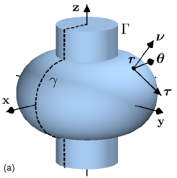
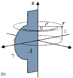
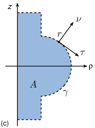
Figure 1: An axisymmetric surface $\Gamma$ generated by a curve $\gamma$. (a) A point ${{\boldsymbol{r}}}$ on $\Gamma$ has outward unit normal $\boldsymbol{\nu}$ and tangential vectors $\boldsymbol{\tau}$ and $\boldsymbol{\theta}$. (b) ${{\boldsymbol{r}}}$ has radial distance $\rho$, azimuthal angle $\theta$, and height $z$. The planar domain $A$ is bounded by $\gamma$ and the $z$-axis. (c) Coordinate axes and vectors in the half-plane $\theta=0$.

The angle $\theta=0$ defines a half-plane in $\mathbb{R}^{3}$ whose intersection with $\Gamma$ corresponds to a generating curve $\gamma$. Let $r=(\rho,z)$ be a point in this half-plane and let $A$ be the planar domain bounded by $\gamma$ and the $z$-axis. The outward unit normal on $\gamma$ is $\nu=(\nu_{\rho},\nu_{z})$ and $\tau=(\nu_{z},-\nu_{\rho})$ is a tangent. See Figure 1(c). The unit vectors in the $\rho$- and $z$-directions are $\hat{\rho}$ and $\hat{z}$.

2.2 PDE formulation

The electric field is scaled with the free space impedance $\eta_{0}$ such that ${\boldsymbol{E}}({\boldsymbol{r}})=\eta_{0}^{-1}{\boldsymbol{E}}^{\prime}({\boldsymbol{r}})$, where ${\boldsymbol{E}}^{\prime}({\boldsymbol{r}})$ is the unscaled field. With vacuum in $V$ and with $\Gamma$ perfectly conducting, the electric field ${\boldsymbol{E}}({\boldsymbol{r}})$ satisfies the system of partial differential equations

$$\nabla^{2}{\boldsymbol{E}}({\boldsymbol{r}})+k^{2}{\boldsymbol{E}}({\boldsymbol{r}}) ={\boldsymbol{0}}\,,\qquad{\boldsymbol{r}}\in V\,,$$ (4)

$$\nabla\cdot{\boldsymbol{E}}({\boldsymbol{r}}) =0\,,\qquad{\boldsymbol{r}}\in V\,,$$ (5)

with boundary condition

$$\lim_{V\ni{\boldsymbol{r}}\to{\boldsymbol{r}}^{\circ}}{\boldsymbol{\nu}}^{\circ}\times{\boldsymbol{E}}({\boldsymbol{r}})={\boldsymbol{0}}\,,\qquad{\boldsymbol{r}}^{\circ}\in\Gamma\,.$$ (6)

We will find nontrivial solutions to these equations in a fast and accurate fashion via the MFIE. Note that, since $\Gamma$ is perfectly conducting and from a mathematical as well as physical point of view, nothing exterior to $\Gamma$ can affect ${\boldsymbol{E}}({\boldsymbol{r}})$ in $V$. Hence the region exterior to $\Gamma$ is irrelevant to the problem.

The values $k^{2}$ for which the system (4), (5), and (6) admits nontrivial solutions are called eigenvalues. We refer to the corresponding fields ${\boldsymbol{E}}({\boldsymbol{r}})$ as electric eigenfields and to $k$ as eigenwavenumbers. The eigenvalues constitute a real, positive, and countable set, accumulating only at infinity [31]. The eigenvalues have finite multiplicity. Electric eigenfields that correspond to distinct eigenvalues are orthogonal with respect to the inner product

$$\langle{\boldsymbol{F}},{\boldsymbol{G}}\rangle=\int_{V}{\boldsymbol{F}}^{\ast}({\boldsymbol{r}})\cdot{\boldsymbol{G}}({\boldsymbol{r}})\,{\rm d}V\,,$$ (7)

where ${\boldsymbol{F}}({\boldsymbol{r}})$ and ${\boldsymbol{G}}({\boldsymbol{r}})$ are vector fields on $V$ and the asterisk indicates the complex conjugate. Subspaces of electric eigenfields that correspond to degenerate eigenvalues can be given orthogonal bases.

Electric eigenfields ${\boldsymbol{E}}({\boldsymbol{r}})$ are normalized so that

$$\|{\boldsymbol{E}}\|^{2}\equiv\int_{V}{\boldsymbol{E}}^{\ast}({\boldsymbol{r}})\cdot{\boldsymbol{E}}({\boldsymbol{r}})\,{\rm d}V=1\,.$$ (8)

The volume integral in (8) is referred to as the normalization integral. In Section 4 it is converted into a surface integral that is well suited for numerical evaluation in the framework of the MFIE.

2.3 Integral representation of the electric field

The surface current density ${\boldsymbol{J}}_{\rm s}$ and the surface charge density $\varrho_{\rm s}$ are defined as

$${\boldsymbol{J}}_{\rm s}({\boldsymbol{r}}^{\circ}) =\frac{{\rm i}}{k}\lim_{V\ni{\boldsymbol{r}}\to{\boldsymbol{r}}^{\circ}}{\boldsymbol{\nu}}^{\circ}\times(\nabla\times{\boldsymbol{E}}({\boldsymbol{r}}))\,,\qquad{\boldsymbol{r}}^{\circ}\in\Gamma\,,$$ (9)

$$\varrho_{\rm s}({\boldsymbol{r}}^{\circ}) =\lim_{V\ni{\boldsymbol{r}}\to{\boldsymbol{r}}^{\circ}}-{\boldsymbol{\nu}}^{\circ}\cdot{\boldsymbol{E}}({\boldsymbol{r}})\,,\qquad{\boldsymbol{r}}^{\circ}\in\Gamma\,.$$ (10)

When ${\boldsymbol{J}}_{\rm s}$ and $\varrho_{\rm s}$ are known the electric field is given by the integral representation

$$\left.\begin{aligned} &{\boldsymbol{E}}({\boldsymbol{r}})\\ &{\boldsymbol{0}}\end{aligned}\right\}={\rm i}k\int_{\Gamma}{\boldsymbol{J}}_{\rm s}({\boldsymbol{r}}^{\prime})\Phi_{k}({\boldsymbol{r}},{\boldsymbol{r}}^{\prime})\,{\rm d}\Gamma^{\prime}-\int_{\Gamma}\varrho_{\rm s}({\boldsymbol{r}}^{\prime})\nabla\Phi_{k}({\boldsymbol{r}},{\boldsymbol{r}}^{\prime})\,{\rm d}\Gamma^{\prime}\left\{\begin{aligned} &{\boldsymbol{r}}\in V\,,\\ &{\boldsymbol{r}}\in c\overline{V}\,,\end{aligned}\right.$$ (11)

where $c\overline{V}$ is the exterior to $V\cup\Gamma$. Here, using the time dependence $e^{-{\rm i}\omega t}$ with angular frequency $\omega>0$, the kernel

$$\Phi_{k}({\boldsymbol{r}},{\boldsymbol{r}}^{\prime})=\frac{e^{{\rm i}k|{\boldsymbol{r}}-{\boldsymbol{r}}^{\prime}|}}{4\pi|{\boldsymbol{r}}-{\boldsymbol{r}}^{\prime}|}$$ (12)

is the causal fundamental solution to the Helmholtz equation and

$$\nabla\Phi_{k}({\boldsymbol{r}},{\boldsymbol{r}}^{\prime})=-\frac{({\boldsymbol{r}}-{\boldsymbol{r}}^{\prime})}{4\pi|{\boldsymbol{r}}-{\boldsymbol{r}}^{\prime}|^{3}}{P(|{\boldsymbol{r}}-{\boldsymbol{r}}^{\prime}|)}\,,$$ (13)

where

$$P(|{\boldsymbol{r}}-{\boldsymbol{r}}^{\prime}|)=(1-{\rm i}k|{\boldsymbol{r}}-{\boldsymbol{r}}^{\prime}|)e^{{\rm i}k|{\boldsymbol{r}}-{\boldsymbol{r}}^{\prime}|}\,.$$ (14)

The lower equation in (11) states that ${\boldsymbol{J}}_{\rm s}$ and $\varrho_{\rm s}$ induce an electric null field outside $\Gamma$.

We decompose the electric field in its cylindrical coordinate components

$${\boldsymbol{E}}({\boldsymbol{r}})={\boldsymbol{\rho}}E_{\rho}({\boldsymbol{r}})+{\boldsymbol{\theta}}E_{\theta}({\boldsymbol{r}})+{\boldsymbol{z}}E_{z}({\boldsymbol{r}})\,$$ (15)

and the surface current density in its tangential components

$${\boldsymbol{J}}_{\rm s}({\boldsymbol{r}})={\boldsymbol{\tau}}J_{\tau}({\boldsymbol{r}})+{\boldsymbol{\theta}}J_{\theta}({\boldsymbol{r}})\,.$$ (16)

From (11) the components of the electric field, including the induced external electric null field, can be expressed as

$$\begin{split}E_{\rho}({\boldsymbol{r}})&={\rm i}kS_{7}J_{\tau}({\boldsymbol{r}})+kS_{8}J_{\theta}({\boldsymbol{r}})+K_{11}\varrho_{\rm s}({\boldsymbol{r}})\,,\\ E_{\theta}({\boldsymbol{r}})&=kS_{9}J_{\tau}({\boldsymbol{r}})+{\rm i}kS_{10}J_{\theta}({\boldsymbol{r}})+{\rm i}K_{12}\varrho_{\rm s}({\boldsymbol{r}})\,,\\ E_{z}({\boldsymbol{r}})&={\rm i}kS_{11}J_{\tau}({\boldsymbol{r}})+K_{13}\varrho_{\rm s}({\boldsymbol{r}})\,,\end{split}$$ (17)

where ${\boldsymbol{r}}\in\mathbb{R}^{3}\setminus\Gamma$ and the double-layer type operators $K_{\alpha}$ and single-layer type operators $S_{\alpha}$ with various indices $\alpha$ are defined by their actions on a layer density $g({{\boldsymbol{r}}})$, ${{\boldsymbol{r}}}\in\Gamma$, as

$$K_{\alpha}g({{\boldsymbol{r}}}) =\int_{\Gamma}K_{\alpha}({\boldsymbol{r}},{\boldsymbol{r}}^{\prime})g({{\boldsymbol{r}}^{\prime}})\,{\rm d}\Gamma^{\prime}\,,$$ (18)

$$K_{\alpha}({\boldsymbol{r}},{\boldsymbol{r}}^{\prime}) =D_{\alpha}({\boldsymbol{r}},{\boldsymbol{r}}^{\prime})P(|{\boldsymbol{r}}-{\boldsymbol{r}}^{\prime}|)\,,$$ (19)

and

$$S_{\alpha}g({{\boldsymbol{r}}}) =\int_{\Gamma}S_{\alpha}({\boldsymbol{r}},{\boldsymbol{r}}^{\prime})g({{\boldsymbol{r}}^{\prime}})\,{\rm d}\Gamma^{\prime}\,,$$ (20)

$$S_{\alpha}({\boldsymbol{r}},{\boldsymbol{r}}^{\prime}) =Z_{\alpha}({\boldsymbol{r}},{\boldsymbol{r}}^{\prime})e^{{\rm i}k|{\boldsymbol{r}}-{\boldsymbol{r}}^{\prime}|}\,.$$ (21)

The functions $D_{\alpha}({\boldsymbol{r}},{\boldsymbol{r}}^{\prime})$ and $Z_{\alpha}({\boldsymbol{r}},{\boldsymbol{r}}^{\prime})$ can be viewed as static kernels, corresponding to wavenumber $k=0$. Their explicit expressions are given in Appendix A.1.

2.4 Integral equations for ${\boldsymbol{J}}_{\rm s}$ and $\varrho_{\rm s}$

The interior MFIE for ${\boldsymbol{J}}_{\rm s}$ reads

$${\boldsymbol{J}}_{\rm s}({\boldsymbol{r}})-2\,{\boldsymbol{\nu}}\times\int_{\Gamma}\left({\boldsymbol{J}}_{\rm s}({\boldsymbol{r}}^{\prime})\times\nabla\Phi_{k}({\boldsymbol{r}},{\boldsymbol{r}}^{\prime})\right)\,{\rm d}\Gamma^{\prime}={\boldsymbol{0}}\,,\qquad{\boldsymbol{r}}\in\Gamma\,.$$ (22)

The surface charge density $\varrho_{\rm s}$ is related to the surface current density ${\boldsymbol{J}}_{\rm s}$ by the continuity equation

$$\varrho_{\rm s}({\boldsymbol{r}})=-\frac{\rm i}{k}\nabla_{\rm s}\cdot{\boldsymbol{J}}_{\rm s}({\boldsymbol{r}})\,,$$ (23)

where $\nabla_{\rm s}\cdot(\;)$ is the surface divergence. As in [20], we avoid the differentiation inherent in (23) by evaluating $\varrho_{\rm s}$ from the interior charge integral equation

$$\varrho_{\rm s}({\boldsymbol{r}})-2\int_{\Gamma}{\boldsymbol{\nu}}\cdot\nabla\Phi_{k}({\boldsymbol{r}},{\boldsymbol{r}}^{\prime})\varrho_{\rm s}({\boldsymbol{r}}^{\prime})\,{\rm d}\Gamma^{\prime}=\\ -2{\rm i}k\int_{\Gamma}{\boldsymbol{\nu}}\cdot{\boldsymbol{J}}_{\rm s}({\boldsymbol{r}}^{\prime})\Phi_{k}({\boldsymbol{r}},{\boldsymbol{r}}^{\prime})\,{\rm d}\Gamma^{\prime}\,,\qquad{\boldsymbol{r}}\in\Gamma\,.$$ (24)

When ${\boldsymbol{J}}_{\rm s}$ and $\varrho_{\rm s}$ are solutions to (22) and (24), then ${\boldsymbol{E}}({\boldsymbol{r}})$ in (11) is a solution to the system (4), (5), and (6).

The Fredholm second kind integral equation (24) and its exterior counterpart are here denoted the ChIE. Over the last decade, the ChIE has become a tool for dealing with certain numerical problems known as “low-frequency breakdown” and which occur when the MFIE, or the related formulations EFIE and CFIE, are used for exterior electromagnetic scattering at low frequencies [29]. Low-frequency breakdown is caused by decoupling of electric and magnetic fields. It manifests itself when integral equations are solved or when fields are reconstructed. More generally, the ChIE has been combined with the MFIE [20, 29], with the EFIE [8], and with the CFIE [4, 28] for PEC surfaces and with the EFIE and the MFIE for penetrable objects [28]. The combination of the MFIE and the ChIE for exterior problems is denoted the ECCIE in [29]. Low-frequency breakdown is not an issue when computing eigenfields since cavity resonances are wave phenomena with a strong coupling between electric and magnetic fields. Our reasons for preferring the ChIE over (23) have, as in [20], to do with convergence order and achievable accuracy.

In accordance with [20] we split (22) into the two coupled scalar equations

$$\begin{split}\left(I+K_{1}\right)J_{\tau}({\boldsymbol{r}})+{\rm i}K_{2}J_{\theta}({\boldsymbol{r}})=0\,,\\ {\rm i}K_{3}J_{\tau}({\boldsymbol{r}})+\left(I+K_{4}\right)J_{\theta}({\boldsymbol{r}})=0\,.\end{split}$$ (25)

and write (24) as

$$(I-2K_{\nu})\varrho_{\rm s}({\boldsymbol{r}})=-2{\rm i}kS_{5}J_{\tau}({\boldsymbol{r}})+2kS_{6}J_{\theta}({\boldsymbol{r}})\,.$$ (26)

Here $I$ is the identity. The operators $K_{\alpha}$, $\alpha=1,2,3,4,\nu$ are of the double-layer type (18) with (19). The operators $S_{5}$ and $S_{6}$ are of the single-layer type (20) with (21). See Appendix A.1 for their explicit expressions.

3 Fourier series expansions

The aim of this paper is to present a high-order convergent and accurate discretization scheme to solve the MFIE and to evaluate electric eigenfields, normalized by (8). We employ a Fourier–Nyström technique where the first step is an azimuthal Fourier transformation of the MFIE system (25) and (26) and of the system for the decomposed electric field (17).

We define the azimuthal Fourier coefficients for 2$\pi$-periodic functions

$$g_{n}(r) =\frac{1}{\sqrt{2\pi}}\int_{-\pi}^{\pi}e^{-{\rm i}n\theta}g({{\boldsymbol{r}}})\,{\rm d}\theta\,,$$ (27)

$$G_{n}(r,r^{\prime}) =\frac{1}{\sqrt{2\pi}}\int_{-\pi}^{\pi}e^{-{\rm i}n(\theta-\theta^{\prime})}G({{\boldsymbol{r}}},{{\boldsymbol{r}}}^{\prime})\,{\rm d}(\theta-\theta^{\prime})\,,$$ (28)

where $g({\boldsymbol{r}})$ represents functions like $\varrho_{\rm s}({\boldsymbol{r}})$, $J_{\tau}({\boldsymbol{r}})$, $J_{\theta}({\boldsymbol{r}})$, $E_{\rho}({\boldsymbol{r}})$, $E_{\theta}({\boldsymbol{r}})$, and $E_{z}({\boldsymbol{r}})$ and where $G({{\boldsymbol{r}}},{{\boldsymbol{r}}}^{\prime})$ represents $K_{\alpha}({{\boldsymbol{r}}},{{\boldsymbol{r}}}^{\prime})$, $D_{\alpha}({{\boldsymbol{r}}},{{\boldsymbol{r}}}^{\prime})$, $S_{\alpha}({{\boldsymbol{r}}},{{\boldsymbol{r}}}^{\prime})$, $Z_{\alpha}({{\boldsymbol{r}}},{{\boldsymbol{r}}}^{\prime})$, and $P(|{{\boldsymbol{r}}}-{{\boldsymbol{r}}}^{\prime}|)$. The subscript $n$ is the azimuthal index, $n=0,\pm 1,\pm 2,\ldots$.

We also define the modal integral operators $K_{\alpha n}$ and $S_{\alpha n}$ in terms of their corresponding Fourier coefficients $K_{\alpha n}(r,r^{\prime})$ and $S_{\alpha n}(r,r^{\prime})$ as

$$K_{\alpha n}g_{n}(r)=\sqrt{2\pi}\int_{\gamma}K_{\alpha n}(r,r^{\prime})g_{n}(r^{\prime})\rho^{\prime}\,{\rm d}\gamma^{\prime}\,,$$ (29)

$$S_{\alpha n}g_{n}(r)=\sqrt{2\pi}\int_{\gamma}S_{\alpha n}(r,r^{\prime})g_{n}(r^{\prime})\rho^{\prime}\,{\rm d}\gamma^{\prime}\,.$$ (30)

Expansion and integration of (25) over $\theta^{\prime}$ now give the system of modal integral equations

$$\begin{split}\left(I+K_{1n}\right)J_{\tau n}(r)+{\rm i}K_{2n}J_{\theta n}(r)=0\,,\\ {\rm i}K_{3n}J_{\tau n}(r)+\left(I+K_{4n}\right)J_{\theta n}(r)=0\,,\end{split}$$ (31)

where $r\in\gamma$. Analogously, the modal version of (26) is

$$\left(I-2K_{{\boldsymbol{\nu}}n}\right)\varrho_{{\rm s}n}(r)=-2{\rm i}kS_{5n}J_{\tau n}(r)+2kS_{6n}J_{\theta n}(r)\,.$$ (32)

The modal representation of the electric field in (17) is

$$\begin{split}E_{\rho n}(r)&={\rm i}kS_{7n}J_{\tau n}(r)+kS_{8n}J_{\theta n}(r)+K_{11n}\varrho_{{\rm s}n}(r)\,,\\ E_{\theta n}(r)&=kS_{9n}J_{\tau n}(r)+{\rm i}kS_{10n}J_{\theta n}(r)+{\rm i}K_{12n}\varrho_{{\rm s}n}(r)\,,\\ E_{zn}(r)&={\rm i}kS_{11n}J_{\tau n}(r)+K_{13n}\varrho_{{\rm s}n}(r)\,,\end{split}$$ (33)

where $r\notin\gamma$.

In what follows, we sometimes present only modal expressions for operators and fields. The reasons being the close resemblance between expressions in $\mathbb{R}^{3}$ and modal expressions, visible in the examples above, and that we seek eigenfields

$${\boldsymbol{E}}_{n}({\boldsymbol{r}})=\left({\boldsymbol{\rho}}E_{\rho n}(r)+{\boldsymbol{\theta}}E_{\theta n}(r)+{\boldsymbol{z}}E_{zn}(r)\right)\frac{e^{{\rm i}n\theta}}{\sqrt{2\pi}}$$ (34)

for one azimuthal mode at a time.

4 Conversion of the normalization integral

The normalization (volume) integral in (8) can be converted into a sum of line integrals over $\gamma$ that is more suitable for numerical evaluation. The line integrals contain Fourier coefficients of an electric scalar potential $\Psi({\boldsymbol{r}})$ and a magnetic vector potential $\boldsymbol{\it\Lambda}({\boldsymbol{r}})$. In [20, Appendix A], using results from [3], this conversion is done in the context of magnetic eigenfields. Since for each eigenwavenumber the electric and magnetic eigenfield energies are equal, the expression in [20] applies equally well to electric eigenfields. With ${\boldsymbol{E}}_{n}({\boldsymbol{r}})$ as in (34) the converted expression reads

$$\|{\boldsymbol{E}}_{n}\|^{2}=k^{2}\int_{A}\left(|\boldsymbol{\it\Lambda}_{n}|^{2}-|\Psi_{n}|^{2}\right)\rho\,{\rm d}A+\int_{\gamma}\left(\boldsymbol{\it\Lambda}_{n}^{\ast}\cdot{\boldsymbol{J}}_{{\rm s}n}+{\rm i}k\Lambda_{\nu n}^{\ast}\Psi_{n}\right)\rho\,{\rm d}\gamma\,,$$ (35)

where

$$k^{2}\int_{A}|\Psi_{n}|^{2}\rho\,{\rm d}A =-\frac{1}{2}\int_{\gamma}\frac{\nu\cdot r}{\rho}\left(n^{2}-k^{2}\rho^{2}\right)|\Psi_{n}|^{2}\,{\rm d}\gamma$$

$$\qquad-\frac{1}{2}\int_{\gamma}\nu\cdot r\left(\left|(\partial_{{\boldsymbol{\tau}}}\Psi)_{n}\right|^{2}-\left|(\partial_{{\boldsymbol{\nu}}^{+}}\Psi)_{n}\right|^{2}\right)\rho\,{\rm d}\gamma$$

$$+\frac{1}{2}\int_{\gamma}{\rm Re}\left\{\left(2\tau\cdot r(\partial_{{\boldsymbol{\tau}}}\Psi^{\ast})_{n}+\Psi^{\ast}_{n}\right)(\partial_{{\boldsymbol{\nu}}^{+}}\Psi)_{n}\right\}\rho\,{\rm d}\gamma\,,$$ (36)

$$k^{2}\int_{A}|\boldsymbol{\it\Lambda}_{n}|^{2}\rho\,{\rm d}A =-\frac{1}{2}\int_{\gamma}\frac{\nu\cdot r}{\rho}\left((n^{2}-k^{2}\rho^{2})|\boldsymbol{\it\Lambda}_{n}|^{2}\right)\,{\rm d}\gamma$$

$$-\frac{1}{2}\int_{\gamma}\frac{\nu\cdot r}{\rho}\left(|\Lambda_{\rho n}|^{2}+|\Lambda_{\theta n}|^{2}-4n\,{\rm Im}\left\{\Lambda_{\rho n}^{\ast}\Lambda_{\theta n}\right\}\right)\,{\rm d}\gamma$$

$$\qquad-\frac{1}{2}\int_{\gamma}\nu\cdot r\left(\left|(\partial_{{\boldsymbol{\tau}}}\boldsymbol{\it\Lambda})_{n}\right|^{2}-\left|(\partial_{{\boldsymbol{\nu}}^{+}}\boldsymbol{\it\Lambda})_{n}\right|^{2}\right)\rho\,{\rm d}\gamma$$

$$+\frac{1}{2}\int_{\gamma}{\rm Re}\left\{(2\tau\cdot r(\partial_{{\boldsymbol{\tau}}}\boldsymbol{\it\Lambda}^{\ast})_{n}+\boldsymbol{\it\Lambda}_{n}^{\ast})\cdot(\partial_{{\boldsymbol{\nu}}^{+}}\boldsymbol{\it\Lambda})_{n}\right\}\rho\,{\rm d}\gamma\,,$$ (37)

and where directional derivatives of a function $g({\boldsymbol{r}})$ are abbreviated as

$$\begin{split}\partial_{{\boldsymbol{\tau}}}g({\boldsymbol{r}})&={\boldsymbol{\tau}}\cdot\nabla g({\boldsymbol{r}})\,,\qquad{\boldsymbol{r}}\in\Gamma\,,\\ \partial_{{\boldsymbol{\nu}}^{+}}g({\boldsymbol{r}}^{\circ})&=\lim_{V\ni{\boldsymbol{r}}\to{\boldsymbol{r}}^{\circ}}{\boldsymbol{\nu}}^{\circ}\cdot\nabla g({\boldsymbol{r}})\,,\qquad{\boldsymbol{r}}^{\circ}\in\Gamma\,.\end{split}$$ (38)

In order to evaluate (35) from the solution to (31) and (32), the Fourier coefficients of $\Psi({\boldsymbol{r}})$ and $\boldsymbol{\it\Lambda}({\boldsymbol{r}})$, and their derivatives with respect to ${\boldsymbol{\tau}}$ and ${\boldsymbol{\nu}}^{+}$, need to be related to $\varrho_{{\rm s}n}(r)$, $J_{\tau n}(r)$, and $J_{\theta n}(r)$. Partial information on these relations, along with derivations, can be found in [20, Appendix B]. We now give complete information without derivations.

Two different decompositions of $\boldsymbol{\it\Lambda}_{n}(r)$ are needed

$$\begin{split}\boldsymbol{\it\Lambda}_{n}(r)&={\boldsymbol{\tau}}\Lambda_{\tau n}(r)+{\boldsymbol{\theta}}\Lambda_{\theta n}(r)+{\boldsymbol{\nu}}\Lambda_{\nu n}(r)\,,\\ \boldsymbol{\it\Lambda}_{n}(r)&={\boldsymbol{\rho}}\Lambda_{\rho n}(r)+{\boldsymbol{\theta}}\Lambda_{\theta n}(r)+{\boldsymbol{z}}\Lambda_{zn}(r)\,.\end{split}$$ (39)

Expressions for $\boldsymbol{\it\Lambda}_{n}(r)$ are in these bases

$$\begin{split}\Lambda_{\tau n}(r)&=S_{1n}J_{\tau n}(r)+{\rm i}S_{2n}J_{\theta n}(r)\,,\\ \Lambda_{\theta n}(r)&={\rm i}S_{3n}J_{\tau n}(r)+S_{4n}J_{\theta n}(r)\,,\\ \Lambda_{\theta 0}(r)&=0\,,\\ \Lambda_{\nu n}(r)&=S_{5n}J_{\tau n}(r)+{\rm i}S_{6n}J_{\theta n}(r)\,,\\ \Lambda_{\rho n}(r)&=S_{12n}J_{\tau n}(r)+{\rm i}S_{13n}J_{\theta n}(r)\,,\\ \Lambda_{zn}(r)&=S_{14n}J_{\tau n}(r)\,.\end{split}$$ (40)

The modal operators $S_{\alpha n}$, $\alpha=1,\ldots,6,12,13,14$, are defined via (30), (28), (21) and Appendix A.1.

Expressions for the Fourier coefficients of the cylindrical components of the derivatives of $\boldsymbol{\it\Lambda}({\boldsymbol{r}})$ with respect to ${\boldsymbol{\tau}}$ and ${\boldsymbol{\nu}}^{+}$ are

$$\begin{split}(\partial_{{\boldsymbol{\tau}}}\boldsymbol{\it\Lambda})_{\rho n}(r)&=K_{14n}J_{\tau n}(r)+{\rm i}K_{15n}J_{\theta n}(r)\,,\\ (\partial_{{\boldsymbol{\tau}}}\boldsymbol{\it\Lambda})_{\theta n}(r)&={\rm i}K_{16n}J_{\tau n}(r)+K_{17n}J_{\theta n}(r)\,,\\ (\partial_{{\boldsymbol{\tau}}}\boldsymbol{\it\Lambda})_{zn}(r)&=K_{18n}J_{\tau n}(r)\,,\\ (\partial_{{\boldsymbol{\nu}}^{+}}\boldsymbol{\it\Lambda})_{\rho n}(r)&=\frac{1}{2}\nu_{z}J_{\tau n}(r)+K_{19n}J_{\tau n}(r)+{\rm i}K_{20n}J_{\theta n}(r)\,,\\ (\partial_{{\boldsymbol{\nu}}^{+}}\boldsymbol{\it\Lambda})_{\theta n}(r)&=\frac{1}{2}J_{\theta n}(r)+{\rm i}K_{21n}J_{\tau n}(r)+K_{22n}J_{\theta n}(r)\,,\\ (\partial_{{\boldsymbol{\nu}}^{+}}\boldsymbol{\it\Lambda})_{zn}(r)&=-\frac{1}{2}\nu_{\rho}J_{\tau n}(r)+K_{23n}J_{\tau n}(r)\,.\end{split}$$ (41)

The modal operators $K_{\alpha n}$, $\alpha=14,\ldots,23$, are defined via (29), (28), (19) and Appendix A.1.

Expressions for the Fourier coefficients of $\Psi({\boldsymbol{r}})$ and its derivatives are [20]

$$\begin{split}\Psi_{n}(r)&=\frac{k}{n}\rho\Lambda_{\theta n}(r)\,,\qquad n\neq 0\,,\\ \Psi_{0}(r)&=S_{\varsigma 0}\varrho_{{\rm s}0}(r)\,,\\ (\partial_{{\boldsymbol{\tau}}}\Psi)_{n}(r)&={\rm i}k\Lambda_{\tau n}(r)\,,\\ (\partial_{{\boldsymbol{\nu}}^{+}}\Psi)_{n}(r)&=\varrho_{{\rm s}n}(r)+{\rm i}k\Lambda_{\nu n}(r)\,,\end{split}$$ (42)

with $S_{\varsigma 0}$ defined via (30), (28), (21) and Appendix A.1.

5 Fourier coefficients of static kernels in analytic form

When $r$ and $r^{\prime}$ are far from each other, all kernels $K_{\alpha}({\boldsymbol{r}},{\boldsymbol{r}}^{\prime})$ and $S_{\alpha}({\boldsymbol{r}},{\boldsymbol{r}}^{\prime})$ are smooth functions of $\theta-\theta^{\prime}$ and we evaluate the corresponding Fourier coefficients $K_{\alpha n}(r,r^{\prime})$ and $S_{\alpha n}(r,r^{\prime})$, needed in (31), (32), (33) and (35), from (28) using discrete Fourier transform techniques (FFT). When $r$ and $r^{\prime}$ are close, the kernels vary more rapidly and FFT alone is not efficient. Instead we split each $K_{\alpha}({\boldsymbol{r}},{\boldsymbol{r}}^{\prime})$ and $S_{\alpha}({\boldsymbol{r}},{\boldsymbol{r}}^{\prime})$ into two parts: a smooth part, which is transformed via FFT, and a rapidly varying part, which is transformed by convolution of $D_{\alpha n}(r,r^{\prime})$ and $Z_{\alpha n}(r,r^{\prime})$ with parts of $P_{n}(r,r^{\prime})$. See [19, Section 6] for details on this splitting and [19, Section 12.1] for a definition of when $r$ and $r^{\prime}$ are considered close.

The coefficients $D_{\alpha n}(r,r^{\prime})$ and $Z_{\alpha n}(r,r^{\prime})$ can be expressed in terms of half-integer degree Legendre functions of the second kind [16, Equation 8.713.1]

$$\mathfrak{Q}_{n-\frac{1}{2}}(\chi)=\int_{-\pi}^{\pi}\frac{\cos(nt)\,{\rm d}t}{\sqrt{8\left(\chi-\cos(t)\right)}}\,.$$ (43)

We use these analytic expressions in the convolutions where, in our setting,

$$\chi=1+\frac{|r-r^{\prime}|^{2}}{2\rho\rho^{\prime}}\,.$$ (44)

The functions $\mathfrak{Q}_{n-\frac{1}{2}}(\chi)$, with real arguments $\chi\geq 1$ and often with $\cosh(\chi)$ substituted for $\chi$, may also be called toroidal functions [16, Section 8.850], [24, page 201], ring functions [1, Section 8.11], or toroidal harmonics [13]. They are symmetric with respect to $n$, exhibit logarithmic singularities at $\chi=1$, and are relatively cheap to evaluate.

The particular combinations of toroidal functions

$$\mathfrak{R}_{n}(\chi)=\frac{2n-1}{\chi+1}\left(\chi\mathfrak{Q}_{n-\frac{1}{2}}(\chi)-\mathfrak{Q}_{n-\frac{3}{2}}(\chi)\right)$$ (45)

play an important role in our analytic expressions. They multiply functions which may exhibit Cauchy-type singularities at $\chi=1$. The $\mathfrak{R}_{n}(\chi)$ are finite at $\chi=1$, but have logarithmic singularities in their first (right) derivatives.

The toroidal functions can be evaluated via a recursion whose forward form is

$$\mathfrak{Q}_{n-\frac{1}{2}}(\chi)=\frac{4n-4}{2n-1}\chi\mathfrak{Q}_{n-\frac{3}{2}}(\chi)-\frac{2n-3}{2n-1}\mathfrak{Q}_{n-\frac{5}{2}}(\chi)\,,\qquad n=2,3,\ldots\,.$$ (46)

When $1<\chi<1.0005$ we use (46) as it stands. When $\chi\geq 1.0005$, and for stability reasons, we use a backward form of (46). A short Matlab code which evaluates $\mathfrak{Q}_{-\frac{1}{2}}(\chi)$ and $\mathfrak{Q}_{\frac{1}{2}}(\chi)$ is presented in [20, Appendix C]. See Appendix A.2 for a complete description of how all coefficients $D_{\alpha n}(r,r^{\prime})$ and $Z_{\alpha n}(r,r^{\prime})$, needed in the present work, are related to $\mathfrak{Q}_{n-\frac{1}{2}}(\chi)$.

6 An overview of the discretization

Our Fourier–Nyström discretization scheme is very similar to the scheme used in [20]. That scheme, in turn, builds on the schemes developed in [19, 32] in a pure Helmholtz setting. This section only gives a brief review.

The FFT operations are, basically, controlled by two problem dependent integers $N$ and $N_{\rm con}$, with $N\geq N_{\rm con}$, as follows: we use $2N+1$ equispaced points in the azimuthal Fourier transforms of kernels when $r$ and $r^{\prime}$ are far from each other, we use $2N_{\rm con}+1-n$ terms in the truncated convolutions [19, Equation (27)], and we use $2N_{\rm con}+1$ equispaced points in the azimuthal Fourier transforms of smooth parts of kernels when $r$ and $r^{\prime}$ are close. The value of $N$ is chosen in an ad hoc manner. The value of $N_{\rm con}$ is determined by the decay of the Fourier coefficients of the test function

$$g(\theta)=\frac{\sin(2k\rho_{\rm max}\sin(\theta/2))}{\sin(\theta/2)}\,,$$ (47)

where $\rho_{\rm max}$ is the largest value of $\rho$ on $\gamma$, so that $N_{\rm con}$ is the number of Fourier coefficients $g_{n}$, $n=1,2,\ldots$, with $g_{n}/g_{0}>10\epsilon_{\rm mach}$. When $r$ and $r^{\prime}$ are in the vicinity of corners, however, we may use smaller values of $N_{\rm con}$. See, further, Section 7.2. We note, but do not generally exploit, that more elaborate adaptivity in the control of the FFT operations can lead to substantial computational savings.

Our Nyström discretization of (31), (32), (33) and (35) relies on an underlying panel-based 16-point Gauss–Legendre quadrature with a mesh of $n_{\rm pan}$ quadrature panels on $\gamma$. The $16n_{\rm pan}$ discretization points play the role of both target points $r_{i}$ and source points $r_{j}$. The underlying quadrature is used in a conventional way when $r_{i}$ and $r_{j}$ are far from each other. When $r_{i}$ and $r_{j}$ are close and convolution is used, see Section 5, an explicit kernel-split special quadrature is activated. Analytical information about the singularities in $K_{\alpha n}(r,r^{\prime})$ and $S_{\alpha n}(r,r^{\prime})$ is exploited in the construction of 16th order accurate weight corrections, computed on the fly. As to some extent compensate for the loss of convergence order that comes with the special quadrature, a procedure of temporary mesh refinement (upsampling) is adopted. See [18] for additional information on quadrature construction and upsampling.

It is worth emphasizing that all $K_{\alpha n}(r,r^{\prime})$ and $S_{\alpha n}(r,r^{\prime})$ contain some sort of singularities at $r=r^{\prime}$ and that these singularities are inherited by the corresponding $D_{\alpha n}(r,r^{\prime})$ and $Z_{\alpha n}(r,r^{\prime})$ listed in Appendix A.2. The singularities are generally of logarithmic type, native to $\mathfrak{Q}_{n-\frac{1}{2}}(\chi)$, with the exceptions that the coefficients in Appendix A.2 that contain the function

$$d(v)=\frac{v\cdot(r-r^{\prime})}{|r-r^{\prime}|^{2}}\,,\qquad v=\tau,\nu,\hat{\rho},\hat{z}\,,$$ (48)

may exhibit Cauchy-type singularities as $r$ approaches $r^{\prime}$ and those coefficients that are proportional to $\mathfrak{R}_{n}(\chi)$ have logarithmic-type singularities only in their first derivatives. The quadratures constructed in [18, 19] cover all these situations.

7 Recursively compressed inverse preconditioning

Spectral properties of integral operators in boundary integral equations are often sensitive to boundary smoothness. The very nature of solutions may be affected by a change in smoothness as may the performance of numerical solvers. For example, the introduction of boundary singularities such as edges and corners can induce diverging asymptotics in layer densities. Intense and costly mesh refinement is then needed for resolution, which may lead to the loss of stability. See [14] for a review of recently developed numerical techniques to deal with this problem.

RCIP is one of the techniques discussed in [14]. It can be viewed as a general method to enhance the performance of panel-based Nyström discretization schemes. Roughly speaking, for Fredholm second kind integral equations, RCIP obtains solutions on piecewise smooth curves with the same accuracy and at about the same cost as with which solutions normally are obtained on smooth curves. The RCIP method originated in 2008 in the context of solving Laplace’s equation in piecewise smooth planar domains [21] and has since then been improved and extended as to apply to a variety of boundary value problems.

A comprehensive description of the RCIP method is given in the tutorial [17]. This section first gives a brief summary and then focuses on some details particular to the MFIE system (31) and (32) and to the converted normalization integral (35) with (36) and (37).

7.1 Basics of the RCIP method

Assume the following: we have an integral representation of a field $U(r)$, $r\in\mathbb{R}^{2}\setminus\gamma$, in terms of an unknown layer density $\sigma(r)$ on a piecewise smooth boundary $\gamma$. On $\gamma$ there are a number $n_{\rm crn}$ of corners with vertices $\gamma_{j}$, $j=1,\ldots,n_{\rm crn}$. The integral representation together with boundary conditions lead to a Fredholm second kind integral equation

$$\left(I+K\right)\sigma(r)=g(r)\,,\qquad r\in\gamma\,,$$ (49)

where $K$ is an integral operator with kernel $K(r,r^{\prime})$ on $\gamma$. The operator $K$ is compact away from the corners. The function $g(r)$ is a right hand side with the same smoothness properties as $\gamma$. We also assume that there is a relatively coarse mesh with $n_{\rm pan}$ coarse quadrature panels of approximately equal length constructed on $\gamma$. The purpose of the coarse mesh is to allow for a discretization that resolves $g(r)$, $\gamma$, and $K(r,r^{\prime})$ for $r$ far away from $r^{\prime}$.

We split the kernel

$$K(r,r^{\prime})=K^{\star}(r,r^{\prime})+K^{\circ}(r,r^{\prime})$$ (50)

in such a way that $K^{\star}(r,r^{\prime})$ is zero except for when $r$ and $r^{\prime}$ both lie within a distance of two coarse quadrature panels from the same $\gamma_{j}$. In this latter case $K^{\circ}(r,r^{\prime})$ is zero. The kernel splitting (50) corresponds to an operator splitting

$$K=K^{\star}+K^{\circ}\,,$$ (51)

where $K^{\circ}$ is a compact operator. The variable substitution

$$\sigma(r)=\left(I+K^{\star}\right)^{-1}\tilde{\sigma}(r)$$ (52)

lets us rewrite (49) as a right preconditioned integral equation

$$\tilde{\sigma}(r)+K^{\circ}(I+K^{\star})^{-1}\tilde{\sigma}(r)=g(r)\,,\qquad r\in\gamma\,,$$ (53)

where the operator composition $K^{\circ}(I+K^{\star})^{-1}$ is compact.

The functions $\tilde{\sigma}(r)$ and $g(r)$ and the operator $K^{\circ}$ in (53) should be easy to discretize and to resolve on the coarse mesh. Only the inverse $(I+K^{\star})^{-1}$ needs a fine mesh for its resolution. This fine mesh is constructed from the coarse mesh by, for each vertex $\gamma_{j}$, choosing a number $n_{{\rm sub}j}$ and letting the panels closest to $\gamma_{j}$ be $n_{{\rm sub}j}$ times repeatedly subdivided. The size of $n_{{\rm sub}j}$ is determined by the behavior of $\sigma(r)$ close to $\gamma_{j}$ and by application-specific needs for resolution. The discretization of (53) can then be carried out as

$$\left({\bf I}_{\rm coa}+{\bf K}_{\rm coa}^{\circ}{\bf R}\right)\tilde{\boldsymbol{\sigma}}_{\rm coa}={\bf g}_{\rm coa}\,,$$ (54)

where the compressed weighted inverse matrix ${\bf R}$ is given by

$${\bf R}={\bf P}_{W}^{T}\left({\bf I}+{\bf K}^{\star}\right)_{\rm fin}^{-1}{\bf P}\,.$$ (55)

In (54) and (55) the subscript “coa” indicates a grid on the coarse mesh, the subscript “fin” indicates a grid on the fine mesh, the prolongation matrix ${\bf P}$ performs polynomial interpolation from the coarse grid to the fine grid and ${\bf P}_{W}^{T}$ is the transpose of a weighted prolongation matrix such that

$${\bf P}_{W}^{T}{\bf P}={\bf I}_{\rm coa}\,.$$ (56)

See [17, Sections 4 and 5] for details. With 16-point composite quadrature the system size in (54) is $16n_{\rm pan}\times 16n_{\rm pan}$. The matrix ${\bf R}$ differs from the identity matrix by having $n_{\rm crn}$ diagonal blocks ${\bf R}^{(j)}$, $j=1,\ldots,n_{\rm crn}$, of size $64\times 64$.

Once (54) is solved for $\tilde{\boldsymbol{\sigma}}_{\rm coa}$, a discrete weight-corrected version of the original layer density is obtained from

$$\hat{\boldsymbol{\sigma}}_{\rm coa}={\bf R}\tilde{\boldsymbol{\sigma}}_{\rm coa}\,.$$ (57)

The density $\hat{\boldsymbol{\sigma}}_{\rm coa}$, together with the composite quadrature, can be used for the accurate discretization of any integral on $\gamma$ involving $\sigma(r)$ and piecewise smooth functions. Furthermore, the field $U(r)$ can now be recovered in those parts of the computational domain that lie away from the vertices $\gamma_{j}$ using $\hat{\boldsymbol{\sigma}}_{\rm coa}$ together with the quadratures of [18, 19] in a discretization of the integral representation for $U(r)$.

Note that in (54), the need for resolution in corners is not visible. The transformed layer density $\tilde{\boldsymbol{\sigma}}_{\rm coa}$ should be as easy to solve for as the original layer density in a discretization of (49) on a smooth $\gamma$. All computational difficulties are gathered in the construction of the matrix ${\bf R}$.

There are $64+32n_{{\rm sub}j}$ discretization points on the fine grid within a distance of two coarse panels from the vertex $\gamma_{j}$. Judging from an inspection of (55) it seems as if computing the matrix block ${\bf R}^{(j)}$ should be an expensive and also unstable undertaking for large $n_{{\rm sub}j}$. Fortunately, ${\bf R}^{(j)}$ can be computed via a fast and stable recursion which relies on hierarchies of small local nested grids around $\gamma_{j}$ and produces hierarchies of matrices ${\bf R}^{(j)}_{i}$, $i=1,\ldots,n_{{\rm sub}j}$, where the last matrix is equal to ${\bf R}^{(j)}$. This fast recursion enables the computation of ${\bf R}^{(j)}$ at a cost only proportional to $n_{{\rm sub}j}$. This is the power of the RCIP method.

The fast recursion for ${\bf R}$ can also be run backwards, acting on $\tilde{\boldsymbol{\sigma}}_{\rm coa}$, for the purpose of reconstructing the solution $\boldsymbol{\sigma}_{\rm fin}$ to a straight-forward discretization of (49) on the fine mesh

$$\left({\bf I}_{\rm fin}+{\bf K}_{\rm fin}\right)\boldsymbol{\sigma}_{\rm fin}={\bf g}_{\rm fin}\,.$$ (58)

By this, one sees that the information contained in $\tilde{\boldsymbol{\sigma}}_{\rm coa}$, together with the ${\bf R}^{(j)}_{i}$, is the same as the information contained in $\boldsymbol{\sigma}_{\rm fin}$. A partial reconstruction of $\boldsymbol{\sigma}_{\rm fin}$ is needed when $U(r)$ is to be evaluated close to the vertices $\gamma_{j}$. See [17, Section 9] for a description of the reconstruction procedure.

7.2 Details particular to the MFIE system

The MFIE system (31) and (32), which on block operator form reads

$$\left[\begin{array}[]{ccc}I-2K_{{\boldsymbol{\nu}}n}&2{\rm i}kS_{5n}&-2kS_{6n}\\ 0&I+K_{1n}&{\rm i}K_{2n}\\ 0&{\rm i}K_{3n}&I+K_{4n}\end{array}\right]\left[\begin{array}[]{c}\varrho_{{\rm s}n}(r)\\ J_{\tau n}(r)\\ J_{\theta n}(r)\end{array}\right]=\left[\begin{array}[]{c}0\\ 0\\ 0\end{array}\right]\,,$$ (59)

has a more complicated appearance than the model equation (49). The operator corresponding to $K^{\star}$ in (51), upon discretization, no longer yields a block diagonal matrix but a sparse block matrix where each vertex $\gamma_{j}$ generates seven non-zero $64\times 64$ blocks. In practice, this poses no problems for RCIP. Equation (54) still holds with

$$\begin{split}&{\bf g}_{\rm coa}={\bf 0}\,,\\ \tilde{\boldsymbol{\sigma}}_{\rm coa}=\left[\begin{array}[]{c}\tilde{\boldsymbol{\varrho}}_{{\rm s}n}\\ \tilde{\bf J}_{\tau n}\\ \tilde{\bf J}_{\theta n}\end{array}\right]_{\rm coa},&\qquad{\bf K}^{\circ}_{\rm coa}=\left[\begin{array}[]{ccc}-2{\bf K}^{\circ}_{{\boldsymbol{\nu}}n}&2{\rm i}k{\bf S}^{\circ}_{5n}&-2k{\bf S}^{\circ}_{6n}\\ {\bf 0}&{\bf K}^{\circ}_{1n}&{\rm i}{\bf K}^{\circ}_{2n}\\ {\bf 0}&{\rm i}{\bf K}^{\circ}_{3n}&{\bf K}^{\circ}_{4n}\end{array}\right]_{\rm coa}.\end{split}$$ (60)

The compressed weighted inverse matrix of (55) is

$${\bf R}=\left[\begin{array}[]{ccc}{\bf P}_{W}&{\bf 0}&{\bf 0}\\ {\bf 0}&{\bf P}_{W}&{\bf 0}\\ {\bf 0}&{\bf 0}&{\bf P}_{W}\end{array}\right]^{T}\\ \left[\begin{array}[]{ccc}{\bf I}-2{\bf K}^{\star}_{{\boldsymbol{\nu}}n}&2{\rm i}k{\bf S}^{\star}_{5n}&-2k{\bf S}^{\star}_{6n}\\ {\bf 0}&{\bf I}+{\bf K}^{\star}_{1n}&{\rm i}{\bf K}^{\star}_{2n}\\ {\bf 0}&{\rm i}{\bf K}^{\star}_{3n}&{\bf I}+{\bf K}^{\star}_{4n}\end{array}\right]^{-1}_{\rm fin}\left[\begin{array}[]{ccc}{\bf P}&{\bf 0}&{\bf 0}\\ {\bf 0}&{\bf P}&{\bf 0}\\ {\bf 0}&{\bf 0}&{\bf P}\end{array}\right]$$ (61)

and has size $48n_{\rm pan}\times 48n_{\rm pan}$. It can be permuted as to differ from the identity matrix by $n_{\rm crn}$ diagonal blocks ${\bf R}^{(j)}$ with $7\times 64\times 64$ non-zero entries each. When computing the ${\bf R}^{(j)}$ via the fast recursion we take advantage of the sparsity structure in (61). We also allow for integers $N_{{\rm con}j}$, controlling FFT operations and convolutions close to the vertices $\gamma_{j}$, that may be smaller than the $N_{\rm con}$ used on the coarse grid. These $N_{{\rm con}j}$ are determined as in Section 6, but with $\rho_{\rm max}$ of (47) replaced with the largest value of $\rho$ on $\gamma$ within a distance of two coarse panels from $\gamma_{j}$.

7.3 Resolving the normalization integral

The RCIP method provides a tool for the fast and accurate solution of the MFIE eigensystem (59) within the framework of our Fourier–Nyström scheme. The discretized equation (54) with (60) and (61) can be used both to find eigenwavenumbers and to find the corresponding discrete transformed eigenvectors, that is, non-trivial solutions. The eigenvectors can, in turn and together with the matrices ${\bf R}^{(j)}_{i}$, be used to reconstruct the discrete densities $\boldsymbol{\varrho}_{{\rm s}n}$, ${\bf J}_{\tau n}$, and ${\bf J}_{\theta n}$ on the fine grid. This is enough to allow for the accurate evaluation of non-normalized electric eigenfields in the entire computational domain, but not enough to allow for the accurate evaluation of normalized eigenfields.

The converted normalization integral (35) with (36) and (37) requires that the Fourier coefficients of $\Psi({\boldsymbol{r}})$ and $\boldsymbol{\it\Lambda}({\boldsymbol{r}})$, and their derivatives with respect to ${\boldsymbol{\tau}}$ and ${\boldsymbol{\nu}}^{+}$, are sufficiently resolved on the fine grid so that their various inner products and squared moduli can be accurately integrated along $\gamma$. For a prescribed overall accuracy and for densities $\varrho_{{\rm s}n}(r)$ or $J_{{\theta n}}(r)$ that diverge at corner vertices, this poses tougher requirements on panel refinement than merely demanding that the densities are sufficiently resolved as to be accurately integrated against piecewise smooth functions. Mappings from partially reconstructed values of $\boldsymbol{\varrho}_{{\rm s}n}$, ${\bf J}_{\tau n}$, and ${\bf J}_{\theta n}$ on the fine grid to values of these sought Fourier coefficients on the fine grid can be performed via hierarchical matrix-vector multiplications similar to, but simpler than, those used for the reconstruction of $\boldsymbol{\varrho}_{{\rm s}n}$, ${\bf J}_{\tau n}$, and ${\bf J}_{\theta n}$ themselves. This procedure uses hierarchies of small matrices corresponding to the evaluation of all modal operators present in (40), (41) and (42) on the small local nested grids mentioned in Section 7.1.

8 Physical fields and edge singularities

This section relates complex valued electric eigenfields in $\mathbb{R}^{3}$ of the form (34) to the physical time-domain standing wave fields that are excited and measured in real life experiments. To facilitate the interpretation of, so called, field maps we also review the leading order asymptotic behavior of electric fields and surface charge and current densities close to edges.

8.1 Physical time-domain fields.

Every eigenvalue $k^{2}$ of the system (4), (5), and (6), not belonging to the mode $n=0$, is degenerate and typically corresponds to a two-dimensional subspace of electric eigenfields. Such an eigenspace can be spanned by two orthonormal eigenfields ${\boldsymbol{E}}_{n}({\boldsymbol{r}})$ and ${\boldsymbol{E}}_{(-n)}({\boldsymbol{r}})$ of the form (34), constructed via (33) from the Fourier coefficients $\varrho_{{\rm s}n}(r)$, $J_{\tau n}(r)$, $J_{\theta n}(r)$ and $\varrho_{{\rm s}(-n)}(r)$, $J_{\tau(-n)}(r)$, $J_{\theta(-n)}(r)$ that are non-trivial solutions to (31) and (32) at eigenwavenumber $k$ and normalized with (8).

The normalized Fourier coefficients are, in turn, unique only up to a constant factor of modulus one. In our implementation we choose these factors such that $J_{\tau n}(r)$ is real and even in $n$, that is, $J_{\tau(-n)}(r)=J_{\tau n}(r)$. Equations (31), (32), (33) and the formulas in Appendix A.2 then imply the following: $J_{\theta n}(r)$ is imaginary and odd in $n$; $E_{\rho n}(r)$, $E_{zn}(r)$, and $\varrho_{{\rm s}n}(r)$ are imaginary and even in $n$; and $E_{\theta n}(r)$ is real and odd in $n$.

Complex valued standing waves are formed by linear combinations of Fourier coefficients as

$$\begin{split}J_{\tau n}^{(\rm e)}({\boldsymbol{r}})&=\frac{a_{n}}{2}(J_{\tau n}(r)e^{{\rm i}n\theta}+J_{\tau(-n)}(r)e^{-{\rm i}n\theta})=a_{n}J_{\tau n}(r)\cos n\theta\,,\\ J_{\tau n}^{(\rm o)}({\boldsymbol{r}})&=-{\rm i}\frac{a_{n}}{2}(J_{\tau n}(r)e^{{\rm i}n\theta}-J_{\tau(-n)}(r)e^{-{\rm i}n\theta})=a_{n}J_{\tau n}(r)\sin n\theta\,,\end{split}$$ (62)

where

$$a_{0}=1/\sqrt{2\pi}\,,\qquad a_{n}=1/\sqrt{\pi}\,,\qquad n=1,2,\ldots\,,$$

and superscript $(\rm e)$ and $(\rm o)$ denote “even” and “odd”. The prefactor $-{\rm i}$ in the second equation of (62) is to make both surface currents real.

The physical time-domain currents in the ${\boldsymbol{\tau}}$-direction are now obtained from

$$\begin{split}J_{\tau n}^{(\rm e)}({\boldsymbol{r}},t)&={\rm Re}\{J_{\tau n}^{(\rm e)}({\boldsymbol{r}})e^{-{\rm i}\omega t}\}=a_{n}J_{\tau n}(r)\cos n\theta\cos\omega t\,,\\ J_{\tau n}^{(\rm o)}({\boldsymbol{r}},t)&={\rm Re}\{J_{\tau n}^{(\rm o)}({\boldsymbol{r}})e^{-{\rm i}\omega t}\}=a_{n}J_{\tau n}(r)\sin n\theta\cos\omega t\,.\end{split}$$ (63)

Expressions for the other physical time-domain quantities are uniquely composed in the same manner as

$$\begin{split}\varrho_{{\rm s}n}^{(\rm e)}({\boldsymbol{r}},t)&=-{\rm i}a_{n}\varrho_{{\rm s}n}(r)\cos n\theta\sin\omega t\,,\\ J_{\theta n}^{(\rm e)}({\boldsymbol{r}},t)&={\rm i}a_{n}J_{\theta n}(r)\sin n\theta\cos\omega t\,,\\ E_{\rho n}^{(\rm e)}({\boldsymbol{r}},t)&=-{\rm i}a_{n}E_{\rho n}(r)\cos n\theta\sin\omega t\,,\\ E_{\theta n}^{(\rm e)}({\boldsymbol{r}},t)&=a_{n}E_{\theta n}(r)\sin n\theta\sin\omega t\,,\\ E_{zn}^{(\rm e)}({\boldsymbol{r}},t)&=-{\rm i}a_{n}E_{zn}(r)\cos n\theta\sin\omega t\,,\end{split}$$ (64)

and

$$\begin{split}\varrho_{{\rm s}n}^{(\rm o)}({\boldsymbol{r}},t)&=-{\rm i}a_{n}\varrho_{{\rm s}n}(r)\sin n\theta\sin\omega t\,,\\ J_{\theta n}^{(\rm o)}({\boldsymbol{r}},t)&=-{\rm i}a_{n}J_{\theta n}(r)\cos n\theta\cos\omega t\,,\\ E_{\rho n}^{(\rm o)}({\boldsymbol{r}},t)&=-{\rm i}a_{n}E_{\rho n}(r)\sin n\theta\sin\omega t\,,\\ E_{\theta n}^{(\rm o)}({\boldsymbol{r}},t)&=-a_{n}E_{\theta n}(r)\cos n\theta\sin\omega t\,,\\ E_{zn}^{(\rm o)}({\boldsymbol{r}},t)&=-{\rm i}a_{n}E_{zn}(r)\sin n\theta\sin\omega t\,.\end{split}$$ (65)

All components of the physical electric eigenfield and its surface charge density are in phase with respect to time, but 90 degrees out of phase with the surface current density. In the numerical examples of Section 9 we present field maps in the $xz$-plane ($\theta=0,\pi$) of the imaginary part of $E_{\rho n}(r)e^{{\rm i}n\theta}$ and $E_{zn}(r)e^{{\rm i}n\theta}$, and the real part of $E_{\theta n}(r)e^{{\rm i}n\theta}$.

8.2 Asymptotic behavior at edges

Let a corner with vertex $\gamma_{j}$ have an (inner) opening angle of $\alpha_{j}$. Let $\xi_{\rm t}$ be the tangential distance from a point $r\in\gamma$ to $\gamma_{j}$ and let $\xi$ be the Euclidean distance from a point $r\in A\cup\Gamma$ to $\gamma_{j}$. For $n>0$, we have the general leading behaviors close to $\gamma_{j}$

$$\begin{split}\varrho_{{\rm s}n}(r)\sim\xi_{\rm t}^{p_{j}-1}\,,\qquad J_{\tau n}(r)\sim 1\,,\qquad J_{\theta n}(r)\sim\xi_{\rm t}^{p_{j}-1}\,,\\ E_{\rho n}(r)\sim\xi^{p_{j}-1}\,,\qquad E_{\theta n}(r)\sim 1\,,\qquad E_{zn}(r)\sim\xi^{p_{j}-1}\,,\end{split}$$ (66)

where

$$p_{j}=\dfrac{\pi}{2\pi-\alpha_{j}}\,.$$ (67)

See [5] and references therein. The asymptotics of the Fourier coefficients of $\Psi({\boldsymbol{r}})$ and $\boldsymbol{\it\Lambda}({\boldsymbol{r}})$, and their derivatives with respect to ${\boldsymbol{\tau}}$ and ${\boldsymbol{\nu}}^{+}$ are more complicated.

For the special case of $n=0$ one can show that (66) holds with some sharpening: the even fields of (64) have $J_{\theta 0}(r)\equiv 0$ and $E_{\theta 0}(r)\equiv 0$; the odd fields of (65) have $\varrho_{{\rm s}0}(r)\equiv 0$, $J_{\tau 0}(r)\equiv 0$, and $E_{\rho 0}(r)=E_{z0}(r)\equiv 0$.

9 Numerical examples

Our Fourier–Nyström scheme for (31), (32), and (33) is implemented in Matlab and executed on a workstation equipped with an Intel Core i7-3930K CPU and 64 GB of memory. The weight corrected densities $\tilde{\boldsymbol{\varrho}}_{{\rm s}n}$, $\tilde{\bf J}_{\tau n}$, and $\tilde{\bf J}_{\theta n}$ on the coarse grid are obtained from (54) with (60) and (61). The densities $\boldsymbol{\varrho}_{{\rm s}n}$, ${\bf J}_{\tau n}$, and ${\bf J}_{\theta n}$ on the fine grid are obtained with reconstruction [17, Section 9]. To enforce (8) we normalize the densities with the value of $\|{\boldsymbol{E}}_{n}\|$ obtained from their insertion in a discretized version of (35).

The Matlab implementation is standard and relies on built-in functions. No particular attempts are made at optimizing the code for speed, except for the use of a few parfor-loops (which execute in parallel). Great care has gone into obtaining intermediate quantities to high accuracy and to resolve modal integral operators in corners. The solution time quoted in the examples below refers to wall-clock time from when an eigenwavenumber is known and until the normalized densities $\boldsymbol{\varrho}_{{\rm s}n}$, ${\bf J}_{\tau n}$, and ${\bf J}_{\theta n}$ are obtained on the fine grid.

9.1 Search for eigenwavenumbers

Eigenwavenumbers are determined using a separate, slimmed down, code that is cleared from matrices and panel refinement only needed for the normalization. In what follows we let $k_{n,j}$ be the $j$th smallest eigenwavenumber for azimuthal index $n$. Our search algorithm for $k_{n,j}$, with $n$ fixed, is a modification of the “standard published method” described in [3, Appendix B]. The standard method is to search along the $k$-axis for (near) zeros of the lowest singular value $s(k)$ of an appropriate discretized system matrix ${\bf B}(k)$. Successive parabolic interpolation, which has convergence rate $r_{\rm c}\approx 1.324$, is applied to $s^{2}(k)$ and is safeguarded by the empirical observation that the slope of $s(k)$ appears to have a domain dependent upper bound $C_{s}$ of size $O(1)$. In our setting, ${\bf B}(k)$ can be taken as the lower right $32n_{\rm pan}\times 32n_{\rm pan}$ part of ${\bf R}^{-1}+{\bf K}_{\rm coa}^{\circ}$ with ${\bf R}$ and ${\bf K}_{\rm coa}^{\circ}$ from (61) and (60).

We modify the standard method, described above, by searching for zeros of the smallest eigenvalue $\lambda(k)$ of ${\bf B}(k)$ rather than for (near) zeros of the smallest singular value. We then replace successive parabolic interpolation applied to $s^{2}(k)$ with the secant method applied to $|\lambda(k)|\operatorname{sgn}(\arg(\lambda(k)))$. The slope of the function $|\lambda(k)|\operatorname{sgn}(\arg(\lambda(k)))$ also appears to have a domain dependent bound of size $O(1)$, which we denote $C_{\lambda}$ and use for safeguarding. The secant method has convergence rate $r_{\rm c}\approx 1.618$. When $C_{\lambda}$ is chosen correctly and for a fixed $n$, our modified search algorithm finds all $k_{n,j}$ in a given $k$-interval typically needing between four and eight iterations per eigenwavenumber found.

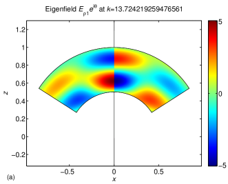
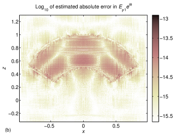
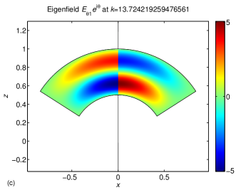
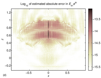
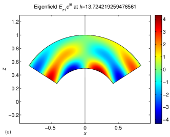
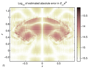
Figure 2: The electric eigenfield at $k_{1,10}=13.724219259476561$ for the cavity with $\gamma$ as in (68). Left: field maps in the $xz$-plane ($\theta=0,\pi$) of (a) ${\rm Im}\left\{E_{\rho 1}(r)e^{{\rm i}\theta}\right\}$, (c) ${\rm Re}\left\{E_{\theta 1}(r)e^{{\rm i}\theta}\right\}$, and (e) ${\rm Im}\left\{E_{z1}(r)e^{{\rm i}\theta}\right\}$. The null-field outside the cavity is omitted. Right: (b), (d), and (f) show $\log_{10}$ of the pointwise absolute difference between the field maps of our scheme and those from the semi-analytic solution. See Section 8 for an explanation of how field maps relate to physical time-domain fields.

9.2 Comparison with solution in semi-analytic form

The codes are first verified for $V$ being the intersection of a cone with half opening angle of one radian and a spherical shell with outer radius one and inner radius 0.5. The generating curve $\gamma$ is parameterized as

$$r(t)=\left\{\begin{array}[]{ll}0.5\left(\sin(2t+2),\cos(2t+2)\right)\,,&t\in[-1,-0.5]\,,\\ (t+1)\left(\sin(1),\cos(1)\right)\,,&t\in[-0.5,0]\,,\\ \left(\sin(1-t),\cos(1-t)\right)\,,&t\in[0,1]\,,\end{array}\right.$$ (68)

and has non-reentrant corners with vertices at $\gamma_{1}=0.5\left(\sin(1),\cos(1)\right)$ and $\gamma_{2}=\left(\sin(1),\cos(1)\right)$. This cavity is an excellent test geometry since, while not trivial, it allows for semi-analytic solutions to the original system (4), (5), and (6). The normalized eigenfields ${\boldsymbol{E}}_{n}({\boldsymbol{r}})$ are expressed in regular and irregular spherical vector waves, see [6, Section 2.2], that are modified to satisfy the boundary condition (6). The major modifications are that the associated Legendre functions $P_{\nu}^{n}(z/|{\boldsymbol{r}}|)$ and spherical Bessel and Neumann functions, $j_{\nu}(k|{\boldsymbol{r}}|)$ and $y_{\nu}(k|{\boldsymbol{r}}|)$ in the vector waves, have indices $\nu$ and wavenumbers $k$ that are solutions to transcendental equations.

Figure 2(a), 2(c), and 2(e) show field maps of $E_{\alpha 1}(r)e^{{\rm i}\theta}$, $\alpha=\rho,\theta,z$, at eigenwavenumber $k_{1,10}=13.724219259476561$ constructed from Fourier coefficients $E_{\alpha 1}(r)$ produced by our codes. The eigenwavenumber corresponds to about 3.7 wavelengths across the generalized diameter of $V$. The Fourier coefficients are obtained with $n_{\rm pan}=28$ quadrature panels, corresponding to 448 discretization points on $\gamma$, and they are evaluated at $245000$ points on a Cartesian grid in the rectangle

$$\Omega_{\rm I}=\left\{r\in\mathbb{R}^{2}:0\leq\rho\leq 0.95\,,-0.45\leq z\leq 1.45\right\}\,.$$ (69)

Only coefficients with $r\in A$ are actually used in Figure 2(a), 2(c), and 2(e). The FFT operations are controlled by the integers $N=141$, $N_{{\rm con}1}=24$, and $N_{{\rm con}2}=N_{\rm con}=30$, see Sections 6 and 7.2. The densities $\varrho_{{\rm s}0}(r)$, $J_{\tau 0}(r)$, and $J_{\theta 0}(r)$ are bounded and the number of panel subdivisions used by the RCIP method for resolution close to $\gamma_{1}$ and $\gamma_{2}$ is chosen as $n_{{\rm sub}1}=n_{{\rm sub}2}=30$, see Section 7.1. The solution time is around 13 seconds and the time required to evaluate the coefficient vector $\left(E_{\rho 1}(r),E_{\theta 1}(r),E_{z1}(r)\right)$ is, on average, 0.002 seconds per point $r$.

Figure 2(b), 2(d), and 2(f) show $\log_{10}$ of the absolute difference between the field maps produced by our codes and the field maps obtained from the semi-analytic solution. Here all coefficients with $r\in\Omega_{\rm I}$ are used. When obtaining the semi-analytic solution, the eigenwavenumber is evaluated to machine precision and the eigenfields to almost machine precision using a combination of Matlab with extended precision and Maple. The semi-analytic solution at points $r$ outside $A\cup\gamma$ is taken as $E_{\alpha 1}(r)=0$, compare (33). One can conclude that, in this example, our codes give coefficients $E_{\alpha 1}(r)$ that are pointwise accurate to at least 13 digits and an eigenwavenumber that is accurate to machine precision.

9.3 The one cell elliptic cavity

Our remaining numerical examples pertain to the cavity depicted in Figure 1 which, in particle accelerator terminology, is known as a one cell elliptic cavity. The generating curve $\gamma$ is parameterized as

$$r(t)=\left\{\begin{array}[]{ll}\left(\pi+t,-1-\pi/4\right)\,,&t\in[-\pi,-3\pi/4]\,,\\ \left(\pi/4,-1+\pi/2+t\right)\,,&t\in[-3\pi/4,-\pi/2]\,,\\ \left(\pi/4+\cos(t),\sin(t)\right)\,,&t\in[-\pi/2,\pi/2]\,,\\ \left(\pi/4,1-\pi/2+t\right)\,,&t\in[\pi/2,3\pi/4]\,,\\ \left(\pi-t,1+\pi/4\right)\,,&t\in[3\pi/4,\pi]\,,\end{array}\right.$$ (70)

and has corner vertices at $\gamma_{1}=(\pi/4,-1-\pi/4)$, $\gamma_{2}=(\pi/4,-1)$, $\gamma_{3}=(\pi/4,1)$, and $\gamma_{4}=(\pi/4,1+\pi/4)$. The corners at $\gamma_{2}$ and $\gamma_{3}$ are reentrant. The number of panel subdivisions in the RCIP method is chosen as $n_{{\rm sub}1}=n_{{\rm sub}4}=30$ and $n_{{\rm sub}2}=n_{{\rm sub}3}=140$ in all examples. The integer $N$, controlling the FFT operations when $r$ and $r^{\prime}$ are far from each other, is by default chosen as $N=4n_{\rm pan}+n$. The estimated pointwise absolute error in a given computed field map is based on a comparison with a more resolved map obtained with 50 per cent more quadrature panels on $\gamma$. Fourier coefficients are evaluated on Cartesian grids in rectangles, most often chosen as

$$\Omega_{\rm II}=\left\{r\in\mathbb{R}^{2}:0\leq\rho\leq 2\,,-2\leq z\leq 2\right\}\,.$$ (71)

Superconducting elliptic cavities are common in linear accelerators for protons. They are to be used in a projected Superconducting Proton Linear accelerator (SPL) at CERN and in the linear accelerator for the European Spallation Source (ESS) that is currently under construction in Lund, Sweden. In the design of elliptic cavities it is important to determine several quantities to high accuracy. For the fundamental eigenfield that accelerates the protons, one needs to evaluate the maximum normalized electric and magnetic fields on the surface and the normalized electric field on the symmetry axis. The eigenfields with azimuthal indices $n=0$ and $n=1$ have non-zero field components on the symmetry axis which cause them to interact with the beam of particles. A large number of these eigenfields have to be determined in order to assess their effect on the beam. The three numerical examples we present for the elliptic cavity have $n=0$ and $n=1$ and eigenwavenumbers that are relevant for particle accelerators.

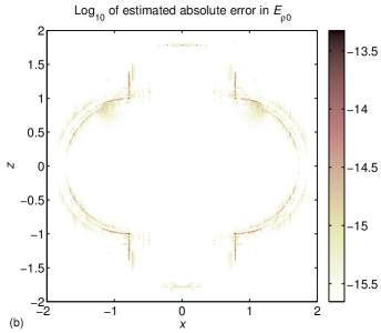
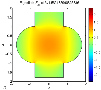
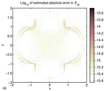
Figure 3: The fundamental electric eigenfield for the elliptic cavity with $\gamma$ as in (70). Left: field maps in the $xz$-plane of (a) ${\rm Im}\left\{E_{\rho 0}(r)\right\}$ and (c) ${\rm Im}\left\{E_{z0}(r)\right\}$. Right: $\log_{10}$ of estimated pointwise absolute error.

9.4 The fundamental mode

The fundamental electric eigenfield is the eigenfield with the lowest eigenwavenumber. For the elliptic cavity with $\gamma$ as in (70) it has eigenwavenumber $k_{0,1}=1.5631689906935362$, corresponding to 0.97 wavelengths across the generalized diameter of $V$. Figure 3(a) and 3(c) show field maps of $E_{\rho 0}(r)$ and $E_{z0}(r)$ as computed with our scheme. The map of $E_{\theta 0}(r)$ is zero and therefore omitted. The Fourier coefficients are obtained with $n_{\rm pan}=32$ quadrature panels, corresponding to 512 discretization points on $\gamma$, and they are evaluated at 245000 points on a grid in $\Omega_{\rm II}$. The FFT operations, for $r$ and $r^{\prime}$ close, are controlled by $N_{{\rm con}1}=N_{{\rm con}4}=12$, $N_{{\rm con}2}=N_{{\rm con}3}=14$ and $N_{\rm con}=16$. The solution time is around 16 seconds and the time required to evaluate the coefficient vector $\left(E_{\rho 0}(r),E_{z0}(r)\right)$ is, on average, 0.003 seconds per point $r$.

Figure 3(b) and 3(d) show $\log_{10}$ of the estimated pointwise absolute error in Figure 3(a) and 3(c). At this low eigenwavenumber the estimated accuracy is quite exceptional. The solver delivers 15 accurate digits except at points close to $\gamma$.

Note that $E_{z0}(r)$ is strong along the symmetry axis. This explains why the fundamental mode is used for acceleration of charged particles. At the vertices of the reentrant corners both $E_{\rho 0}(r)$ and $E_{z0}(r)$ diverge as $\xi^{-1/3}$, see Section 8.2. In the design of de facto elliptic cavities in accelerators, sharp reentrant cell- and iris edges are avoided. On the other hand, there are sharp reentrant edges where the beam pipe is attached to the cavity and it is therefore important that a solver can handle all sorts of sharp edges. We have omitted the beam pipe in order to keep the model simple.

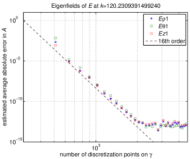
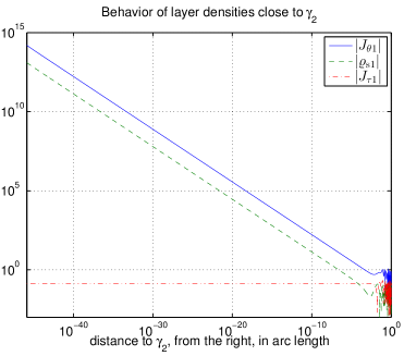
Figure 4: Left: convergence of $E_{\rho 1}(r)$, $E_{\theta 1}(r)$, and $E_{z1}(r)$ with $\gamma$ given by (70) and at eigenwavenumber $k_{1,9928}=120.2309391499240$. The estimated average pointwise absolute error in $A$ has converged to less than $10^{-12}$ at $1920$ discretization points on $\gamma$, corresponding to 16 points per wavelength along $\gamma$. Right: behavior of $\varrho_{{\rm s}1}(r)$, $J_{\tau 1}(r)$, and $J_{\theta 1}(r)$ close to $\gamma_{2}$.

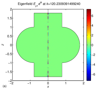
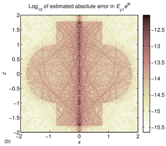
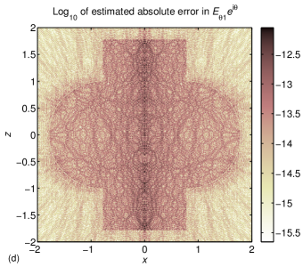
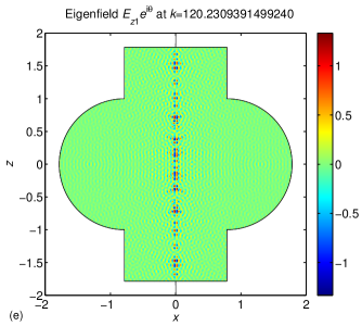
Figure 5: The electric eigenfield for the elliptic cavity with $\gamma$ as in (70) and with $k_{1,9928}=120.2309391499240$. Left: field maps in the $xz$-plane of (a) ${\rm Im}\left\{E_{\rho 1}(r)e^{{\rm i}\theta}\right\}$, (c) ${\rm Re}\left\{E_{\theta 1}(r)e^{{\rm i}\theta}\right\}$, and (e) ${\rm Im}\left\{E_{z1}(r)e^{{\rm i}\theta}\right\}$. Right: $\log_{10}$ of estimated pointwise absolute error.

9.5 A convergence study

The next example is the eigenfield with $k_{1,9928}=120.2309391499240$. Despite a generalized diameter of the elliptic cavity that now corresponds to around 75 wavelengths, our solver maintains 16th order convergence and high achievable accuracy, as seen in the left image of Figure 4. The FFT operations are in this study controlled by $N=\max\{300,4n_{\rm pan}+n\}$, $N_{{\rm con}1}=N_{{\rm con}4}=127$, $N_{{\rm con}2}=N_{{\rm con}3}=137$, and $N_{\rm con}=259$. The Fourier coefficients are evaluated at 45000 points on a grid in $\Omega_{\rm II}$ and have converged to more than 12 digits already at 16 points per wavelength along $\gamma$, which is marginally better than in a similar study for the eigenfield with $k_{1,2460}=60.21392380136615$ (not shown). We conclude that there are no signs of any pollution effect [2] at these wavenumbers.

The right image of Figure 4 reveals that at the reentrant corners both $\varrho_{{\rm s}1}(r)$ and $J_{\theta 1}(r)$ diverge as $\xi_{\rm t}^{-1/3}$, whereas $J_{\tau 1}(r)$ is bounded. These asymptotics are in accordance with (66).

Figure 5 shows fully converged field maps of $E_{\alpha 1}(r)e^{{\rm i}\theta}$, $\alpha=\rho,\theta,z$, obtained with 2816 discretization points on $\gamma$, along with $\log_{10}$ of estimated pointwise absolute error. The solution time is around 240 seconds and the time required to evaluate the coefficient vector $\left(E_{\rho 1}(r),E_{\theta 1}(r),E_{z1}(r)\right)$ is, on average, 0.04 seconds per point $r$. One can see, in the left images, that the eigenfield is concentrated to a region close to the symmetry axis. This is typical for eigenfields with small $n$ and large $k$.

It follows from (10) that the normal component of the coefficient vector has the same (singular) behavior as $\varrho_{{\rm s}1}(r)$ along $\gamma$. The amplitude of a singularity in $\varrho_{{\rm s}1}(r)$ in a reentrant corner is often small at large eigenwavenumbers. As seen in the right image of Figure 4, it may become visible first at a distance from a corner vertex that is less than one thousandth of the total arclength. Although the images of Figure 5 use 245000 evaluation points on the grid in $\Omega_{\rm II}$, this is not enough to detect the singularities in the field maps. This underscores the importance of being able to zoom regions where singularities might appear in order to determine their amplitudes.

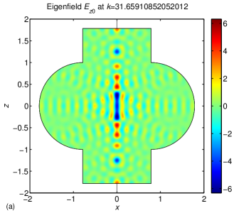
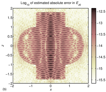
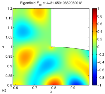
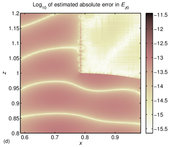
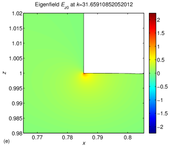
Figure 6: The electric eigenfield for the elliptic cavity with $\gamma$ as in (70) and with $k_{0,662}=31.65910852052012$. Left: (a) the field map of ${\rm Im}\left\{E_{z0}(r)\right\}$ in the $xz$-plane, (c) is a ten times and (e) a 100 times magnification in the vicinity of the corner vertex $\gamma_{3}$. Right: $\log_{10}$ of estimated pointwise absolute error.

9.6 Corner zoom

Our last example is the eigenfield with $k_{0,662}=31.65910852052012$. This eigenfield is even according to the classification of Section 8.1 and has $E_{\theta 0}(r)=0$ in agreement with Section 8.2. Figure 6(a) shows a field map of $E_{z0}(r)$ obtained with 768 discretization points on $\gamma$, $N_{{\rm con}1}=N_{{\rm con}4}=48$, $N_{{\rm con}2}=N_{{\rm con}3}=57$, and $N_{\rm con}=85$ and evaluated at 245000 points on a grid in $\Omega_{\rm II}$. The solution time is around 37 seconds.

Figure 6(c) and 6(e) explore the field map of $E_{z0}(r)$ when the region around the corner vertex $\gamma_{3}$ is magnified first ten times and then 100 times. There are still 768 discretization points on $\gamma$, but field evaluations now take place at 490000 points on grids in the squares

$$\Omega_{\delta}=\left\{r\in\mathbb{R}^{2}:\frac{\pi}{4}-\delta\leq\rho\leq\frac{\pi}{4}+\delta\,,1-\delta\leq\ z\leq 1+\delta\right\}\,,$$ (72)

where $\delta=0.2$ or $\delta=0.02$. At $\gamma_{3}$ (and at $\gamma_{2}$) the field map of $E_{z0}(r)$ exhibits the singularity given by (66). The right images of Figure 6 show $\log_{10}$ of the estimated pointwise absolute error.

This example emphasizes that high accuracy is vital for the detection of singular fields. A less accurate solver might neglect strong local electric fields that can lead to serious electric discharges in a cavity.

10 Conclusion and outlook

We have presented a competitive solver for the determination of normalized electric eigenfields in axially symmetric microwave cavities with piecewise smooth PEC surfaces. The solver is based on the following key elements: the interior magnetic field integral equation, a charge integral equation, a surface integral for normalization, a high-order convergent Fourier–Nyström discretization scheme, on-the-fly computation of singular and nearly singular quadrature rules, and access to high-order surface information.

While our solver determines eigenfields with extraordinary accuracy for a large range of eigenwavenumbers, we observe that the development of efficient high-order Nyström schemes for time-harmonic boundary value problems in piecewise smooth three-dimensional domains is an active research field. See [7] for a recent example of a fast solver for the integral equations which model low-frequency acoustic scattering from curved surfaces.

The computational needs in accelerator technology are extensive and our solver must be equipped with additional features to become a truly versatile tool. Our next step is to allow for sources, modeling a pulsed beam of particles, inside cavities. This makes it possible to evaluate wakefields generated by beams in accelerators. We foresee that our solver can be used for benchmarking. It will be able to evaluate high-frequency parts of wakefield spectra that other solvers cannot reach and by that it becomes an important complement to state-of-the-art software such as the CST Particle Studio Wakefield Solver. We also anticipate other improvements. The present Matlab implementation places emphasis on high achievable accuracy and on rapid convergence with respect to the degrees of freedom. For this, modal integral operators are upsampled in a somewhat crude and costly way. Better adaptivity in this process and in the FFT operations will lead to increased execution speed.

Nano-optics is another application that involves high-frequency electromagnetic eigenfields. Here structures that support whispering gallery modes (WGMs) are of great interest [27]. The WGMs have large eigenwavenumbers and large azimuthal indices and the numerical examples presented in [20] indicate that our solver is ideal for their evaluation. When the WGM structures are dielectric bodies of revolution, the solver needs to be adapted to a similar set of integral equations as in [9]. The WGM structures used in nano-optics are designed to have very high Quality factors (Q-factors), and the bandwidth of such structures is very small since the Q-factor equals the frequency-to-bandwidth ratio. There are reported Q-factors as high as $10^{11}$ [27] with a relative bandwidth of $10^{-11}$. In principle, a solver that delivers eleven digit accuracy is needed to design such a structure if a WGM of the structure is to be excited by a laser with a given wavelength.

Appendix A Explicit expressions for kernels

The various double- and single-layer type operators $K_{\alpha}$ and $S_{\alpha}$ used in this paper are defined by their corresponding static kernels $D_{\alpha}({\boldsymbol{r}},{\boldsymbol{r}}^{\prime})$ and $Z_{\alpha}({\boldsymbol{r}},{\boldsymbol{r}}^{\prime})$ via (18) with (19) and (20) with (21). This appendix collects explicit expressions for all static kernels along with analytic expressions for their Fourier coefficients $D_{\alpha n}(r,r^{\prime})$ and $Z_{\alpha n}(r,r^{\prime})$. The numbering of the operators and kernels is compatible with the numbering used in [20]. Note that for azimuthal index $n=0$ the modal operators $K_{2n}$, $K_{3n}$, $K_{12n}$, $K_{15n}$, $K_{16n}$, $K_{20n}$, $K_{21n}$, $S_{2n}$, $S_{3n}$, $S_{6n}$, $S_{8n}$, $S_{9n}$, and $S_{13n}$ are zero.

A.1 Static kernels

The static kernels are expressed in terms of the azimuthal angle $\theta$ and vectors and points in the plane defined by $\theta=0$, see Section 2.1. The abbreviations

$${\boldsymbol{\nu}}\cdot({\boldsymbol{r}}-{\boldsymbol{r}}^{\prime})=\nu\cdot(r-r^{\prime})+\nu_{\rho}\rho^{\prime}(1-\cos(\theta-\theta^{\prime}))\,,$$

$${\boldsymbol{\tau}}\cdot({\boldsymbol{r}}-{\boldsymbol{r}}^{\prime})=\tau\cdot(r-r^{\prime})+\nu_{z}\rho^{\prime}(1-\cos(\theta-\theta^{\prime}))\,,$$

$$|{\boldsymbol{r}}-{\boldsymbol{r}}^{\prime}|=\left(\rho^{2}+\rho^{\prime 2}-2\rho\rho^{\prime}\cos(\theta-\theta^{\prime})+(z-z^{\prime})^{2}\right)^{\frac{1}{2}}\,,$$

$$\Phi_{0}({\boldsymbol{r}},{\boldsymbol{r}}^{\prime})=\frac{1}{4\pi|{\boldsymbol{r}}-{\boldsymbol{r}}^{\prime}|}\,,\qquad\tilde{\Phi}_{0}^{3}({\boldsymbol{r}},{\boldsymbol{r}}^{\prime})=\frac{1}{4\pi|{\boldsymbol{r}}-{\boldsymbol{r}}^{\prime}|^{3}}\,,$$

are used. The static double-layer type kernels are

$$D_{{\boldsymbol{\nu}}}({\boldsymbol{r}},{\boldsymbol{r}}^{\prime}) =-{\boldsymbol{\nu}}\cdot({\boldsymbol{r}}-{\boldsymbol{r}}^{\prime})\tilde{\Phi}_{0}^{3}({\boldsymbol{r}},{\boldsymbol{r}}^{\prime})\,,$$

$$D_{1}({\boldsymbol{r}},{\boldsymbol{r}}^{\prime}) =2\left(\nu_{\rho}^{\prime}\rho-(\nu^{\prime}\cdot r^{\prime}-\nu_{z}^{\prime}z)\cos(\theta-\theta^{\prime})\right)\tilde{\Phi}_{0}^{3}({\boldsymbol{r}},{\boldsymbol{r}}^{\prime})\,,$$

$$D_{2}({\boldsymbol{r}},{\boldsymbol{r}}^{\prime}) =-2{\rm i}(z-z^{\prime})\sin(\theta-\theta^{\prime})\tilde{\Phi}_{0}^{3}({\boldsymbol{r}},{\boldsymbol{r}}^{\prime})\,,$$

$$D_{3}({\boldsymbol{r}},{\boldsymbol{r}}^{\prime}) =2{\rm i}(\nu_{z}^{\prime}\nu\cdot r-\nu_{z}\nu^{\prime}\cdot r^{\prime})\sin(\theta-\theta^{\prime})\tilde{\Phi}_{0}^{3}({\boldsymbol{r}},{\boldsymbol{r}}^{\prime})\,,$$

$$D_{4}({\boldsymbol{r}},{\boldsymbol{r}}^{\prime}) =-2\left(\nu_{\rho}\rho^{\prime}-(\nu\cdot r-\nu_{z}z^{\prime})\cos(\theta-\theta^{\prime})\right)\tilde{\Phi}_{0}^{3}({\boldsymbol{r}},{\boldsymbol{r}}^{\prime})\,,$$

$$D_{11}({\boldsymbol{r}},{\boldsymbol{r}}^{\prime}) =\left(\rho-\rho^{\prime}\cos(\theta-\theta^{\prime})\right)\tilde{\Phi}_{0}^{3}({\boldsymbol{r}},{\boldsymbol{r}}^{\prime})\,,$$

$$D_{12}({\boldsymbol{r}},{\boldsymbol{r}}^{\prime}) =-{\rm i}\rho^{\prime}\sin(\theta-\theta^{\prime})\tilde{\Phi}_{0}^{3}({\boldsymbol{r}},{\boldsymbol{r}}^{\prime})\,,$$

$$D_{13}({\boldsymbol{r}},{\boldsymbol{r}}^{\prime}) =(z-z^{\prime})\tilde{\Phi}_{0}^{3}({\boldsymbol{r}},{\boldsymbol{r}}^{\prime})\,,$$

$$D_{14}({\boldsymbol{r}},{\boldsymbol{r}}^{\prime}) =-{\boldsymbol{\tau}}\cdot({\boldsymbol{r}}-{\boldsymbol{r}}^{\prime})\nu^{\prime}_{z}\cos(\theta-\theta^{\prime})\tilde{\Phi}_{0}^{3}({\boldsymbol{r}},{\boldsymbol{r}}^{\prime})\,,$$

$$D_{15}({\boldsymbol{r}},{\boldsymbol{r}}^{\prime}) ={\rm i}{\boldsymbol{\tau}}\cdot({\boldsymbol{r}}-{\boldsymbol{r}}^{\prime})\sin(\theta-\theta^{\prime})\tilde{\Phi}_{0}^{3}({\boldsymbol{r}},{\boldsymbol{r}}^{\prime})\,,$$

$$D_{16}({\boldsymbol{r}},{\boldsymbol{r}}^{\prime}) =-{\rm i}{\boldsymbol{\tau}}\cdot({\boldsymbol{r}}-{\boldsymbol{r}}^{\prime})\nu^{\prime}_{z}\sin(\theta-\theta^{\prime})\tilde{\Phi}_{0}^{3}({\boldsymbol{r}},{\boldsymbol{r}}^{\prime})\,,$$

$$D_{17}({\boldsymbol{r}},{\boldsymbol{r}}^{\prime}) =-{\boldsymbol{\tau}}\cdot({\boldsymbol{r}}-{\boldsymbol{r}}^{\prime})\cos(\theta-\theta^{\prime})\tilde{\Phi}_{0}^{3}({\boldsymbol{r}},{\boldsymbol{r}}^{\prime})\,,$$

$$D_{18}({\boldsymbol{r}},{\boldsymbol{r}}^{\prime}) ={\boldsymbol{\tau}}\cdot({\boldsymbol{r}}-{\boldsymbol{r}}^{\prime})\nu^{\prime}_{\rho}\tilde{\Phi}_{0}^{3}({\boldsymbol{r}},{\boldsymbol{r}}^{\prime})\,,$$

$$D_{19}({\boldsymbol{r}},{\boldsymbol{r}}^{\prime}) =-{\boldsymbol{\nu}}\cdot({\boldsymbol{r}}-{\boldsymbol{r}}^{\prime})\nu^{\prime}_{z}\cos(\theta-\theta^{\prime})\tilde{\Phi}_{0}^{3}({\boldsymbol{r}},{\boldsymbol{r}}^{\prime})\,,$$

$$D_{20}({\boldsymbol{r}},{\boldsymbol{r}}^{\prime}) ={\rm i}{\boldsymbol{\nu}}\cdot({\boldsymbol{r}}-{\boldsymbol{r}}^{\prime})\sin(\theta-\theta^{\prime})\tilde{\Phi}_{0}^{3}({\boldsymbol{r}},{\boldsymbol{r}}^{\prime})\,,$$

$$D_{21}({\boldsymbol{r}},{\boldsymbol{r}}^{\prime}) =-{\rm i}{\boldsymbol{\nu}}\cdot({\boldsymbol{r}}-{\boldsymbol{r}}^{\prime})\nu^{\prime}_{z}\sin(\theta-\theta^{\prime})\tilde{\Phi}_{0}^{3}({\boldsymbol{r}},{\boldsymbol{r}}^{\prime})\,,$$

$$D_{22}({\boldsymbol{r}},{\boldsymbol{r}}^{\prime}) =-{\boldsymbol{\nu}}\cdot({\boldsymbol{r}}-{\boldsymbol{r}}^{\prime})\cos(\theta-\theta^{\prime})\tilde{\Phi}_{0}^{3}({\boldsymbol{r}},{\boldsymbol{r}}^{\prime})\,,$$

$$D_{23}({\boldsymbol{r}},{\boldsymbol{r}}^{\prime}) ={\boldsymbol{\nu}}\cdot({\boldsymbol{r}}-{\boldsymbol{r}}^{\prime})\nu^{\prime}_{\rho}\tilde{\Phi}_{0}^{3}({\boldsymbol{r}},{\boldsymbol{r}}^{\prime})\,.$$

The static single-layer type kernels are

$$Z_{\varsigma}({\boldsymbol{r}},{\boldsymbol{r}}^{\prime}) =\Phi_{0}({\boldsymbol{r}},{\boldsymbol{r}}^{\prime})$$

$$Z_{1}({\boldsymbol{r}},{\boldsymbol{r}}^{\prime}) =\left(\nu_{z}\nu_{z}^{\prime}\cos(\theta-\theta^{\prime})+\nu_{\rho}\nu_{\rho}^{\prime}\right)\Phi_{0}({\boldsymbol{r}},{\boldsymbol{r}}^{\prime})\,,$$

$$Z_{2}({\boldsymbol{r}},{\boldsymbol{r}}^{\prime}) =-{\rm i}\nu_{z}\sin(\theta-\theta^{\prime})\Phi_{0}({\boldsymbol{r}},{\boldsymbol{r}}^{\prime})\,,$$

$$Z_{3}({\boldsymbol{r}},{\boldsymbol{r}}^{\prime}) ={\rm i}\nu_{z}^{\prime}\sin(\theta-\theta^{\prime})\Phi_{0}({\boldsymbol{r}},{\boldsymbol{r}}^{\prime})\,,$$

$$Z_{4}({\boldsymbol{r}},{\boldsymbol{r}}^{\prime}) =\cos(\theta-\theta^{\prime})\Phi_{0}({\boldsymbol{r}},{\boldsymbol{r}}^{\prime})\,,$$

$$Z_{5}({\boldsymbol{r}},{\boldsymbol{r}}^{\prime}) =\left(\nu_{\rho}\nu_{z}^{\prime}\cos(\theta-\theta^{\prime})-\nu_{z}\nu_{\rho}^{\prime}\right)\Phi_{0}({\boldsymbol{r}},{\boldsymbol{r}}^{\prime})\,,$$

$$Z_{6}({\boldsymbol{r}},{\boldsymbol{r}}^{\prime}) =-{\rm i}\nu_{\rho}\sin(\theta-\theta^{\prime})\Phi_{0}({\boldsymbol{r}},{\boldsymbol{r}}^{\prime})\,,$$

$$Z_{7}({\boldsymbol{r}},{\boldsymbol{r}}^{\prime}) =\nu^{\prime}_{z}\cos(\theta-\theta^{\prime})\Phi_{0}({\boldsymbol{r}},{\boldsymbol{r}}^{\prime})\,,$$

$$Z_{8}({\boldsymbol{r}},{\boldsymbol{r}}^{\prime}) ={\rm i}\sin(\theta-\theta^{\prime})\Phi_{0}({\boldsymbol{r}},{\boldsymbol{r}}^{\prime})\,,$$

$$Z_{9}({\boldsymbol{r}},{\boldsymbol{r}}^{\prime}) =-Z_{3}({\boldsymbol{r}},{\boldsymbol{r}}^{\prime})\,,$$

$$Z_{10}({\boldsymbol{r}},{\boldsymbol{r}}^{\prime}) =Z_{4}({\boldsymbol{r}},{\boldsymbol{r}}^{\prime})\,,$$

$$Z_{11}({\boldsymbol{r}},{\boldsymbol{r}}^{\prime}) =-\nu^{\prime}_{\rho}\Phi_{0}({\boldsymbol{r}},{\boldsymbol{r}}^{\prime})\,,$$

$$Z_{12}({\boldsymbol{r}},{\boldsymbol{r}}^{\prime}) =Z_{7}({\boldsymbol{r}},{\boldsymbol{r}}^{\prime})\,,$$

$$Z_{13}({\boldsymbol{r}},{\boldsymbol{r}}^{\prime}) =-Z_{8}({\boldsymbol{r}},{\boldsymbol{r}}^{\prime})\,,$$

$$Z_{14}({\boldsymbol{r}},{\boldsymbol{r}}^{\prime}) =Z_{11}({\boldsymbol{r}},{\boldsymbol{r}}^{\prime})\,.$$

A.2 Fourier coefficients

Our derivation of the Fourier coefficients of the static kernels is made in a similar manner as in Young, Hao, and Martinsson [32, Section 5.3]. The idea to expand the Green’s function for the Laplacian in the functions $\mathfrak{Q}_{n-\frac{1}{2}}(\chi)$ comes from Cohl and Tohline [10]. We use the notation of Sections 2.1 and 5 with $\chi$ as in (44) and

$$\eta =\left(8\pi^{3}\rho\rho^{\prime}\right)^{-\frac{1}{2}}\,,$$

$$d(v) =\frac{v\cdot(r-r^{\prime})}{|r-r^{\prime}|^{2}}\,,$$

$$\mathfrak{P}_{n}(\chi) =\frac{1}{2}\left(\mathfrak{R}_{n}(\chi)+\mathfrak{Q}_{n-\frac{1}{2}}(\chi)\right)\,,$$

$$\mathfrak{M}_{n}(\chi) =\chi\mathfrak{Q}_{n-\frac{1}{2}}(\chi)-\frac{\chi+1}{4n^{2}-1}\mathfrak{R}_{n}(\chi)\,,$$

$$\mathfrak{D}_{n}(\chi) =\frac{2n(\chi+1)}{4n^{2}-1}\mathfrak{R}_{n}(\chi)\,,$$

$$\mathfrak{L}_{n}(\chi) =\mathfrak{R}_{n}(\chi)+2(\chi-1)\mathfrak{P}_{n}(\chi)\,,$$

$$\mathfrak{C}_{n}(\chi) =2n(\chi-1)\mathfrak{Q}_{n-\frac{1}{2}}(\chi)\,.$$

The Fourier coefficients of the static double-layer type kernels are

$$D_{{\boldsymbol{\nu}}n}(r,r^{\prime}) =\eta\left[d(\nu)\mathfrak{R}_{n}(\chi)-\frac{\nu_{\rho}}{\rho}\mathfrak{P}_{n}(\chi)\right]\,,$$

$$D_{1n}(r,r^{\prime}) =-2\eta\left[d(\nu^{\prime})\mathfrak{R}_{n}(\chi)-\frac{\left(\nu^{\prime}\cdot r^{\prime}-\nu^{\prime}_{z}z\right)}{\rho\rho^{\prime}}\mathfrak{P}_{n}(\chi)\right]\,,$$

$$D_{2n}(r,r^{\prime}) =-2\eta\frac{\left(z-z^{\prime}\right)}{\rho\rho^{\prime}}n\mathfrak{Q}_{n-\frac{1}{2}}(\chi)\,,$$

$$D_{3n}(r,r^{\prime}) =2\eta\frac{\left(\nu_{z}^{\prime}\nu\cdot r-\nu_{z}\nu^{\prime}\cdot r^{\prime}\right)}{\rho\rho^{\prime}}n\mathfrak{Q}_{n-\frac{1}{2}}(\chi)\,,$$

$$D_{4n}(r,r^{\prime}) =-2\eta\left[d(\nu)\mathfrak{R}_{n}(\chi)+\frac{\left(\nu\cdot r-\nu_{z}z^{\prime}\right)}{\rho\rho^{\prime}}\mathfrak{P}_{n}(\chi)\right]\,,$$

$$D_{11n}(r,r^{\prime}) =-\eta\left[d(\hat{\rho})\mathfrak{R}_{n}(\chi)-\frac{1}{\rho}\mathfrak{P}_{n}(\chi)\right]\,,$$

$$D_{12n}(r,r^{\prime}) =-\frac{\eta}{\rho}n\mathfrak{Q}_{n-\frac{1}{2}}(\chi)\,,$$

$$D_{13n}(r,r^{\prime}) =-\eta\,d(\hat{z})\mathfrak{R}_{n}(\chi)\,,$$

$$D_{14n}(r,r^{\prime}) =\eta\,\nu^{\prime}_{z}\left[d(\tau)\mathfrak{L}_{n}(\chi)-\frac{\nu_{z}}{2\rho}\left(\mathfrak{L}_{n}(\chi)+\mathfrak{M}_{n}(\chi)\right)\right]\,,$$

$$D_{15n}(r,r^{\prime}) =\eta\left[d(\tau)\mathfrak{C}_{n}(\chi)-\frac{\nu_{z}}{2\rho}\left(\mathfrak{C}_{n}(\chi)+\mathfrak{D}_{n}(\chi)\right)\right]\,,$$

$$D_{16n}(r,r^{\prime}) =-\eta\,\nu^{\prime}_{z}\left[d(\tau)\mathfrak{C}_{n}(\chi)-\frac{\nu_{z}}{2\rho}\left(\mathfrak{C}_{n}(\chi)+\mathfrak{D}_{n}(\chi)\right)\right]\,,$$

$$D_{17n}(r,r^{\prime}) =\eta\left[d(\tau)\mathfrak{L}_{n}(\chi)-\frac{\nu_{z}}{2\rho}\left(\mathfrak{L}_{n}(\chi)+\mathfrak{M}_{n}(\chi)\right)\right]\,,$$

$$D_{18n}(r,r^{\prime}) =-\eta\,\nu^{\prime}_{\rho}\left[d(\tau)\mathfrak{R}_{n}(\chi)-\frac{\nu_{z}}{\rho}\mathfrak{P}_{n}(\chi)\right]\,,$$

$$D_{19n}(r,r^{\prime}) =\eta\,\nu^{\prime}_{z}\left[d(\nu)\mathfrak{L}_{n}(\chi)-\frac{\nu_{\rho}}{2\rho}\left(\mathfrak{L}_{n}(\chi)+\mathfrak{M}_{n}(\chi)\right)\right]\,,$$

$$D_{20n}(r,r^{\prime}) =\eta\left[d(\nu)\mathfrak{C}_{n}(\chi)-\frac{\nu_{\rho}}{2\rho}\left(\mathfrak{C}_{n}(\chi)+\mathfrak{D}_{n}(\chi)\right)\right]\,,$$

$$D_{21n}(r,r^{\prime}) =-\eta\,\nu^{\prime}_{z}\left[d(\nu)\mathfrak{C}_{n}(\chi)-\frac{\nu_{\rho}}{2\rho}\left(\mathfrak{C}_{n}(\chi)+\mathfrak{D}_{n}(\chi)\right)\right]\,,$$

$$D_{22n}(r,r^{\prime}) =\eta\left[d(\nu)\mathfrak{L}_{n}(\chi)-\frac{\nu_{\rho}}{2\rho}\left(\mathfrak{L}_{n}(\chi)+\mathfrak{M}_{n}(\chi)\right)\right]\,,$$

$$D_{23n}(r,r^{\prime}) =-\eta\,\nu^{\prime}_{\rho}\left[d(\nu)\mathfrak{R}_{n}(\chi)-\frac{\nu_{\rho}}{\rho}\mathfrak{P}_{n}(\chi)\right]\,.$$

The Fourier coefficients of the static single-layer type kernels are

$$Z_{\varsigma n}(r,r^{\prime}) =\eta\,\mathfrak{Q}_{n-\frac{1}{2}}(\chi)\,,$$

$$Z_{1n}(r,r^{\prime}) =\eta\left[\nu_{z}\nu^{\prime}_{z}\mathfrak{M}_{n}(\chi)+\nu_{\rho}\nu^{\prime}_{\rho}\mathfrak{Q}_{n-\frac{1}{2}}(\chi)\right]\,,$$

$$Z_{2n}(r,r^{\prime}) =\eta\,\nu_{z}\mathfrak{D}_{n}(\chi)\,,$$

$$Z_{3n}(r,r^{\prime}) =-\eta\,\nu^{\prime}_{z}\mathfrak{D}_{n}(\chi)\,,$$

$$Z_{4n}(r,r^{\prime}) =\eta\,\mathfrak{M}_{n}(\chi)\,,$$

$$Z_{5n}(r,r^{\prime}) =\eta\left[\nu_{\rho}\nu^{\prime}_{z}\mathfrak{M}_{n}(\chi)-\nu_{z}\nu^{\prime}_{\rho}\mathfrak{Q}_{n-\frac{1}{2}}(\chi)\right]\,,$$

$$Z_{6n}(r,r^{\prime}) =\eta\,\nu_{\rho}\mathfrak{D}_{n}(\chi)\,,$$

$$Z_{7n}(r,r^{\prime}) =\eta\,\nu^{\prime}_{z}\mathfrak{M}_{n}(\chi)\,,$$

$$Z_{8n}(r,r^{\prime}) =-\eta\,\mathfrak{D}_{n}(\chi)\,,$$

$$Z_{9n}(r,r^{\prime}) =-Z_{3n}(r,r^{\prime})\,,$$

$$Z_{10n}(r,r^{\prime}) =Z_{4n}(r,r^{\prime})\,,$$

$$Z_{11n}(r,r^{\prime}) =-\eta\,\nu^{\prime}_{\rho}\mathfrak{Q}_{n-\frac{1}{2}}(\chi)\,,$$

$$Z_{12n}(r,r^{\prime}) =Z_{7n}(r,r^{\prime})\,,$$

$$Z_{13n}(r,r^{\prime}) =-Z_{8n}(r,r^{\prime})\,,$$

$$Z_{14n}(r,r^{\prime}) =Z_{11n}(r,r^{\prime})\,.$$

References

- [1] M. Abramowitz and I.A. Stegun, Handbook of mathematical functions with formulas, graphs, and mathematical Tables, Dover Publications, New York, 1972.
- [2] I. M. Babuška and S. A. Sauter, “Is the pollution effect of the FEM avoidable for the Helmholtz equation considering high wave numbers?”, SIAM J. Numer. Anal., 34 (1997) 2392–2423.
- [3] A. H. Barnett and A. Hassell, “Fast computation of high-frequency Dirichlet eigenmodes via spectral flow of the interior Neumann-to-Dirichlet map”, Comm. Pure Appl. Math., 67 (2014) 351–407.
- [4] A. Bendali, F. Collino, M. Fares and B. Steif, “Extension to nonconforming meshes of the combined current and charge integral equation”, IEEE Trans. Antennas Propag., 60 (2012) 4732–4744.
- [5] M. M. Bibby, A. F. Peterson, and C. M. Coldwell, “High order representations for singular currents at corners”, IEEE Trans. Antennas Propag., 56 (2008) 2277–2287.
- [6] A. Boström, G. Kristensson, and S. Ström, “Transformation properties of plane, spherical and cylindrical scalar and vector wave functions”, in Field Representations and Introduction to Scattering, V. V. Varadan, A. Lakhtakia, and V. K. Varadan, eds., Acoustic, Electromagnetic and Elastic Wave Scattering 1, pp. 165–210, North–Holland, Amsterdam, 1991.
- [7] J. Bremer, A. Gillman, and P. G. Martinsson, “A high-order accurate accelerated direct solver for acoustic scattering from surfaces”, BIT Numer. Math., 55 (2015) 367–397.
- [8] J. Bremer and Z. Gimbutas, “On the numerical evaluation of the singular integrals of scattering theory”, J. Comput. Phys., 251 (2013) 327–343.
- [9] V. S. Bulygin, Y. V. Gandel, A. Vukovic, T. M. Benson, P. Sewell, and A. I. Nosich, “Nystrom method for the Muller boundary integral equations on a dielectric body of revolution: axially symmetric problem”, IET Microw. Antenna. P., 9 (2015) 1186–1192.
- [10] H. S. Cohl and J. E. Tohline, “A compact cylindrical Green’s function expansion for the solution of potential problems”, Astrophys. J., 527 (1999) 86–101.
- [11] J. L. Fleming, A. W. Wood, and W. D. Wood Jr., “Locally corrected Nyström method for EM scattering by bodies of revolution”, J. Comput. Phys., 196 (2004) 41–52.
- [12] S. D. Gedney and R. Mittra, “The use of the FFT for the efficient solution of the problem of electromagnetic scattering by a body of revolution”, IEEE Trans. Antennas Propag., 38 (1990) 313–322.
- [13] A. Gil, J. Segura, and N. M. Temme, “Computing toroidal functions for wide ranges of the parameters”, J. Comput. Phys., 161 (2000) 204–217.
- [14] A. Gillman, S. Hao, P. G. Martinsson, “A simplified technique for the efficient and highly accurate discretization of boundary integral equations in 2D on domains with corners”, J. Comput. Phys., 256 (2014) 214–219.
- [15] A. W. Glisson and D. R. Wilton, “Simple and efficient numerical techniques for treating bodies of revolution”, Univ. Mississippi Phase Rep. RADC-TR-79-22, 1979.
- [16] I. S. Gradsteyn and I. M. Ryzhik, Table of Integrals, Series, and Products, 7th ed., Elsevier, Amsterdam, 2007.
- [17] J. Helsing, “Solving integral equations on piecewise smooth boundaries using the RCIP method: a tutorial”, Abstr. Appl. Anal., 2013 (2013) Article ID 938167.
- [18] J. Helsing and A. Holst, “Variants of an explicit kernel-split panel-based Nyström discretization scheme for Helmholtz boundary value problems”, Adv. Comput. Math., 41 (2015) 691–708.
- [19] J. Helsing and A. Karlsson, “An explicit kernel-split panel-based Nyström scheme for integral equations on axially symmetric surfaces”, J. Comput. Phys., 272 (2014) 686–703.
- [20] J. Helsing and A. Karlsson, “Determination of normalized magnetic eigenfields in microwave cavities”, IEEE Trans. Microwave Theory Tech., 63 (2015) 1457–1467.
- [21] J. Helsing and R. Ojala, “Corner singularities for elliptic problems: Integral equations, graded meshes, quadrature, and compressed inverse preconditioning”, J. Comput. Phys., 227 (2008) 8820 – 8840.
- [22] M. Idemen, “Confluent edge conditions for the electromagnetic wave at the edge of a wedge bounded by material sheets”, Wave Motion, 32 (2000) 37–55.
- [23] A. M. Linkov and V. F. Koshelev, “Multi-wedge points and multi-wedge elements in computational mechanics: evaluation of exponent and angular distribution”, Int. J. Solids Struct., 43 (2006) 5909–5930.
- [24] W. Magnus, F. Oberhettinger, and R. P. Soni, Formulas and Theorems for the Special Functions of Mathematical Physics, 3rd ed., Springer, Berlin, 1966.
- [25] J. R. Mautz and R. F. Harrington, “Radiation and scattering from bodies of revolution”, Appl. Sci. Res., 20 (1969) 405–435.
- [26] H. Padamsee, J. Knobloch and T. Hays, RF Superconductivity for Accelerators, 2nd ed., Wiley-VCH, Weinheim, 2008.
- [27] G. C. Righini, Y. Dumeige, P. Féron, M. Ferrari, G. Nunzi Conti, D. Ristic, and S. Soria , “Whispering gallery mode microresonators: fundamentals and applications”, Riv. Nuovo Cimento 34 (2011) 435–488.
- [28] M. Taskinen and P. Ylä-Oijala, “ Current and charge integral equation formulation”, IEEE Trans. Antennas Propag., 54 (2006) 58–67.
- [29] F. Vico, Z. Gimbutas, L. Greengard, and M. Ferrando-Bataller, “Overcoming low-frequency breakdown of the magnetic field integral equation”, IEEE Trans. Antennas Propag., 61 (2013) 1285–1290.
- [30] T. P. Wangler, RF Linear accelerators, 2nd ed., Wiley-VCH, Weinheim, 2008.
- [31] G. Wen, “Time-domain theory of metal cavity resonator”, Prog. Electromagn. Res., 78 (2008) 219–253.
- [32] P. Young, S. Hao, and P.G. Martinsson, “A high-order Nyström discretization scheme for boundary integral equations defined on rotationally symmetric surfaces”, J. Comput. Phys., 231 (2012) 4142–4159.