Thomas Bläsius and Annette Karrer†
and Ignaz RutterDepartment of Theoretical Informatics,
Karlsruhe Institute of Technology (KIT) blaesius@kit.edu,
annette.karrer@student.kit.eduDepartment of Theoretical Informatics,
Karlsruhe Institute of Technology (KIT), Karlsruhe and Department
of Applied Mathematics, Charles University, Prague.
rutter@kit.edu. Work was supported by a fellowship
within the Postdoc-Program of the German Academic Exchange Service
(DAAD).
Abstract
A simultaneous embedding (with fixed edges) of two graphs
and with common graph is a pair of planar
drawings of and that coincide on . It is an open
question whether there is a polynomial-time algorithm that decides
whether two graphs admit a simultaneous embedding (problem
Sefe).
In this paper, we present two results. First, a set of three
linear-time preprocessing algorithms that remove certain
substructures from a given Sefe instance, producing a set of
equivalent Sefe instances without such substructures. The
structures we can remove are (1) cutvertices of the union
graph , (2) most separating pairs of
, and (3) connected components of that are biconnected
but not a cycle.
Second, we give an -time algorithm solving Sefe for
instances with the following restriction. Let be a pole of a
P-node in the SPQR-tree of a block of or . Then at
most three virtual edges of may contain common edges incident
to . All algorithms extend to the sunflower case, i.e., to the
case of more than three graphs pairwise intersecting in the same
common graph.
1 Introduction
A simultaneous embedding of two graphs and with common
graph is a pair of planar drawings of
and , that coincide on . The problem to decide whether a
simultaneous embedding exists is called Sefe (Simultaneous
Embedding with Fixed Edges). This definition extends to more than two
graphs. For three graphs Sefe is
NP-complete [11]. In the sunflower case it is
required that every pair of input graphs has the same intersection.
See [3] for a survey on Sefe and related
problems.
There are two fundamental approaches to solving Sefe in the
literature. The first approach is based on the characterization of
Jünger and Schulz [15] stating that finding a
simultaneous embedding of two graphs and with common graph
is equivalent to finding planar embeddings of and that
induce the same embedding on . The second very recent approach by
Schaefer [17] is based on Hanani-Tutte-style redrawing
results. One tries to characterize the existence of a Sefe via
the existence of drawings of the union graph where no two
independent edges of the same graph cross an odd number of times. The
existence of such drawings can be expressed using a linear system of
boolean equations.
When following the first approach, we need two things to describe the
planar embedding of the common graph . First, for each vertex ,
a cyclic order of incident edges around . Second, for every pair
of connected components and of , the face of
containing . We call this relationship the relative
position of with respect to . To find a simultaneous
embedding, one needs to find a pair of planar embeddings that induce
the same cyclic edge orderings (consistent edge orderings) and
the same relative positions (consistent relative positions) on
the common graph .
Most previous results use the first approach but none of them
considers both consistent edge orderings and relative positions. Most
of them assume the common graph to be connected or to contain no
cycles. The strongest results of this type are the two linear-time
algorithms for the case that is biconnected by Haeupler et
al. [13] and by Angelini et al. [1]
and a quadratic-time algorithm for the case where and are
biconnected and is connected [4]. In the latter
result, Sefe is modeled as an instance of the problem
Simultaneous PQ-Ordering. On the other hand, there is a
linear-time algorithm for Sefe if the common graph consists
of disjoint cycles [7], which requires to ensure
consistent relative positions but makes edge orderings trivially
consistent.
The advantage of the second approach (Hanani-Tutte) is that it
implicitly handles both, consistent edge orderings and consistent
relative positions, at the same time. Thus, the results by
Schaefer [17] are the first that handle Sefe
instances where the common graph consists of several, non-trivial
connected components. He gives a polynomial-time algorithm for the
cases where each connected component of the common graph is
biconnected or has maximum degree 3. Although this approach is
conceptionally simple, very elegant, and combines several notions of
planarity within a common framework, it has two disadvantages. The
running time of the algorithms are quite high and the high level of
abstraction makes it difficult to generalize the results.
Contribution & Outline.
In this paper, we follow the first approach and show how to enforce
consistent edge orderings and consistent relative positions at the
same time, by combining different recent approaches, namely the
algorithm by Angelini et al. [1], the result on
Simultaneous PQ-Ordering [4] for consistent
edge orderings, and the result on disjoint cycles [7]
for consistent relative positions. Note that the relative positions
of connected components to each other are usually expressed in terms
of faces (containing the respective component). This is no longer
possible if the embeddings, and thus the set of faces, of connected
components are not fixed. To overcome this issue, we show that these
relative positions can be expressed in terms of relative positions
with respect to a cycle basis. In addition to that, we are able to
handle certain cutvertices of and .
More precisely, we classify a vertex to be a union
cutvertex, a simultaneous cutvertex, and an exclusive
cutvertex if is a cutvertex of , of and but
not of , and of but not or the other way around,
respectively. Similarly, we can define union separating
pairs to be separating pairs in . We present several
preprocessing algorithms that simplify given instances of Sefe;
see Section 3. Besides a very technical
preprocessing step (Section 3.4),
they remove union cutvertices and most (but not all) union separating
pairs; see Theorem 3, and
replace connected components of that are biconnected with cycles.
They run in linear time and can be applied independently. The latter
algorithm together with the linear-time algorithm for disjoint
cycles [7] improves the result by
Schaefer [17] for instances where every connected component
of is biconnected to linear time.
In Section 5 we show how to solve instances
that have common P-node degree 3 and simultaneous cutvertices
of common degree at most 3 in cubic time. A vertex has common
degree if it is a common vertex with degree in . An
instance has common P-node degree if, for each pole of a
P-node (of a block) of the input graphs, at most virtual
edges of contain common edges incident to . This result
relies heavily on the preprocessing algorithms excluding certain
structures. Together with the preprocessing steps, this includes the
case where every connected component of is biconnected, has
maximum degree 3, or is outerplanar with maximum degree 3 cutvertices.
As before, this approach also applies to the sunflower case.
We would like to point out that the conference version of this article
contained a flaw in the handling of relative positions that are
determined by P-nodes. It was erroneously claimed that certain
constraints could be expressed in terms of linear Equations over
. The issue has been fixed by an additional
preprocessing step (see
Section 3.4), which allows to
exclude the problematic case when treating relative positions decided
by P-nodes. See Section 5.4 for additional
details.
2 Preliminaries
Connectivity & SPQR-trees.
A graph is connected if there exists a path between any pair of
vertices. A separating -set is a set of vertices whose
removal disconnects the graph. Separating 1-sets and 2-sets are
cutvertices and separating pairs, respectively. A
connected graph is biconnected if it has no cut vertex and
triconnected if it has no separating pair. The maximal
biconnected components of a graph are called blocks. The
split components with respect to a separating -set are the
maximal subgraphs that are not disconnected by removing the separating
-set.
The SPQR-tree of a biconnected graph represents the
decomposition of along its split pairs, where a split pair
is either a separating pair or a pair of adjacent
vertices [9]. It can be computed in linear
time [12].
Let be a split pair and let and be two
subgraphs of such that and . Consider the tree consisting of two nodes and
associated with the graphs and , respectively.
These graphs are called skeletons of the nodes , denoted
by , and the special edge is a virtual edge.
Let and be the virtual edges connecting
and in and , respectively. The
two edges and are twins and denote this
relationship by (and vice versa). We say
that the neighbor of corresponding to the virtual edge
is . Conversely, corresponds to the virtual
edge in . In this way, the edge between and
represents the twin-relationship between and
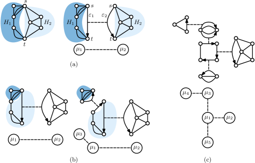
; see Figure 1a for an example. We can
iterate this decomposition process on the graphs and
; see Figure 1b.
Figure 1: (a) A single decomposition step with respect to the split
pair . (b) Continued decomposition. (c) The final
SPQR-tree.
Applying this kind of decomposition systematically yields the
SPQR-tree ; see Figure 1c. The skeletons of the
internal nodes of are either a cycle (S-node), a bunch of
parallel edges (P-node) or a triconnected planar graph (R-node). All
edges in these skeletons are virtual edges. The leaves are Q-nodes
and their skeleton consists of two vertices connected by a virtual and
a normal edge. Sometimes it is more convenient to consider SPQR-trees
without their Q-nodes. In this case, the P-, S-, and R-nodes can also
contain non-virtual edges (as in Figure 1c).
When we choose a planar embedding for the skeleton of each node of the
SPQR-tree , this induces a planar embedding for .
Conversely, fixing the planar embedding of determines the
embeddings of all skeletons. Thus, the combination of all planar
embeddings of all skeletons is in one-to-one correspondence with the
planar embeddings of . Hence, the SPQR-tree breaks the complicated
embedding choices for (on the sphere, i.e., up to the choice of
the outer face) down to embedding choices of the skeletons. These
remaining choices are very simple. Skeletons of S-nodes are cycles
and thus have a unique planar embedding. For P-nodes we can reorder
the parallel edges arbitrarily and the embedding of R-node skeletons
is fixed up to a flip (i.e., up to mirroring the embedding).
Assume is rooted at an arbitrary node. In this case, the
skeleton of every node (except for the root) has a unique virtual edge
corresponding to its parent in . We call this virtual
edge the parent edge and its endpoints the poles. We
recursively define the pertinent graph of a node of
. If is a Q-node, its pertinent graph is the
non-virtual edge in . If is an inner node, the
pertinent graph of is obtained by deleting the parent edge in
and replacing each remaining virtual edge with the
pertinent graph of the corresponding child.
Let be a virtual edge in and let be the
corresponding neighbor of . The expansion graph
of is the pertinent graph of when
choosing as root. Note that the expansion and pertinent graphs
are very similar concepts. However, in most cases we use the
expansion graph as it is independent of the root of the SPQR-tree (and
is still defined if is unrooted). Intuitively, the
expansion graph of a virtual edge is the graph that is represented by
that virtual edge. Note that replacing every virtual edge in
(for any node of ) with its expansion
graph yields the graph . A vertex in is an
inner vertex if it is not an endvertex of .
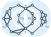
Figure 2: A P-node of with virtual edges . The node has common P-node degree ; for the
virtual edges , , and count; for the
virtual edges , , and count.
Let be the SPQR-tree of a block of in an instance of
Sefe and let be the common graph. Let further be a
P-node of . We say that has common P-node degree
if both vertices in are incident to common edges in
the expansion graphs of at most virtual edges (note that these can
be different edges for the two vertices); see
Figure 2 for an example. We say that
has common P-node degree if each P-node in the SPQR-tree of each
block of has common P-node degree . If this is the case for
and , we say that the instance of Sefe has common
P-node degree .
We use the following conventions to make handling SPQR-trees more
convenient. In most cases (as above) we explicitly name the
SPQR-trees we consider (e.g., , or ). However,
sometimes it is more convenient to write to denote the
SPQR-tree of a given graph . The SPQR-tree is only defined for
biconnected graphs. With the SPQR-tree of a non-biconnected graph, we
implicitly mean a collection of SPQR-trees, one for each block. For
an S-, P-, Q-, or R-node of the SPQR-tree of a graph , we
also say that is an S-, P-, Q-, or R-node of , respectively.
These conventions for example simplify the statement “let be a
P-node of the SPQR-tree of a block of ” to “let be a P-node
of ”.
PQ-trees.
A PQ-tree, originally introduced by Booth and
Lueker [8], is a tree, whose inner nodes are either
P-nodes or Q-nodes (note that these P-nodes have nothing to do with
the P-nodes of the SPQR-tree). The order of edges around a P-node can
be chosen arbitrarily, the edges around a Q-node are fixed up to a
flip. In this way, a PQ-tree represents a set of orders on its
leaves. A rooted PQ-tree represents linear orders, an unrooted
PQ-tree represents cyclic orders (in most cases we consider unrooted
PQ-trees). Given a PQ-tree and a subset of its leaves, there
exists another PQ-tree representing exactly the orders
represented by where the elements in are consecutive. The
tree is the reduction of with respect to . The
projection of to is a PQ-tree with leaves
representing exactly the orders on that are represented by .
The problem Simultaneous PQ-Ordering has several PQ-trees as
input that are related by identifying some of their
leaves [4]. More precisely, every instance is a
directed acyclic graph, where each node is a PQ-tree, and each arc
has the property that there is an injective map from the
leaves of the child to the leaves of the parent
. For each PQ-tree in such an instance, one wants to find an order
of its leaves such that for every arc the order chosen for
the parent is an extension of the order chosen for the child
(with respect to the injective map). We will later use instances of
Simultaneous PQ-Ordering to express relations between orderings
of edges around vertices.
3 Preprocessing Algorithms
In this section, we present several algorithms that can be used as a
preprocessing of a given Sefe instance. The result is usually a
set of Sefe instances that admit a solution if and only if the
original instance admits one. The running time of the preprocessing
algorithms is linear, and so is the total size of the equivalent set
of Sefe instances. Each of the preprocessing algorithms removes
certain types of structures form the instance, in particular from the
common graph. Namely, we show that we can eliminate union
cutvertices, simultaneous cutvertices with common-degree 3, and
connected components of that are biconnected but not a cycle.
None of these algorithms introduces new cutvertices in or
increases the degree of a vertex. Thus, the preprocessing
algorithms can be successively applied to a given instance, removing
all the claimed structures.
Let be a Sefe instance with common graph . We can equivalently encode such an instance in terms of its
union graph , whose edges are
labeled , , or , depending on whether they are
contained exclusively in , exclusively in , or in ,
respectively. Any graph with such an edge coloring can be considered
as a Sefe instance. Since sometimes the coloring version is
more convenient, we use these notions interchangeably throughout this
section.
3.1 Union Cutvertices
Recall that a union cutvertex of a Sefe instance is
a cutvertex of the union graph . The following theorem states
that the Sefe instances corresponding to the split components of
a cutvertex of can be solved independently; see
Figure 3.
Figure 3: A union cutvertex separates a Sefe instance into
independent subinstances.
Lemma 1.
Let be a Sefe instance and let be a cutvertex
of with split components . Then
admits a Sefe if and only if admits a Sefe
for .
Proof.
Clearly, a Sefe of contains a Sefe
of . Conversely, given a Sefe of
for , we can assume without loss of generality that
is incident to the outer face in each of the . Then these
embeddings can be merged to a Sefe of .
∎
Due to Lemma 1, it suffices to consider the blocks
of of a Sefe instance independently. Clearly, the
blocks can be computed in time, and, given a Sefe for
each block, a Sefe of the original instance can be computed
in time.
Theorem 1.
There is a linear-time algorithm that decomposes a Sefe
instance into an equivalent set of Sefe instances that do not
contain union cutvertices.
3.2 Union Separating Pairs
In analogy to a union cutvertex, we can define a union
separating pair to be a separating pair of the union graph
. It is tempting to proceed as for the union cutvertices:
separate according to a union separating pair, solve the
subinstances corresponding to the resulting subgraphs, and merge the
partial solutions.
However, this approach fails as merging the partial solutions may be
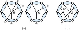
impossible; see Figure 4a. Note that it is
easy to merge the partial solutions if all of them have and on
the outer face of their union graph. One can enforce this kind of
behaviour by connecting and with a common edge in each
subinstance. Unfortunately, this is too restrictive as the
subinstances may fail to have a Sefe with this additional
edge whereas the original instance has a solution; see
Figure 4b.
Figure 4: (a) The original instance does not admit a Sefe
but the split components with respect to the separating pair (marked vertices) do. (b) The original instance admits a
Sefe but one of the split components does not when adding
the common edge .
We can, however, use the idea of adding the common edge in every
subinstance to get rid of most union separating pairs. Throughout the
whole section, we restrict our considerations to the case that and
are vertices of the same block of the common graph and that
is a separating pair in . If separates
into three or more split components, then and are poles of a
P-node of . The case when there are only two split
components is a somewhat special (less interesting) case. To achieve
a more concise notation, we thus assume in the following that and
are the poles of a P-node. However, all arguments extend to the
special case with two split components.
Let be the P-node of with poles and .
Two virtual edges and of are
linked in if contains a path from an inner vertex
in to an inner vertex in that is
disjoint from (except for the end vertices of the path). The
-link graph of has the virtual
edges of as nodes, with an edge between two nodes if and only if
the corresponding virtual edges are linked in . Analogously, we
can define the -link graph and the
union-link graph .
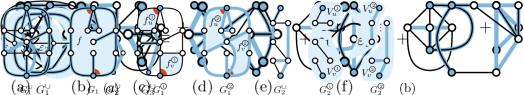
Figure 5: A P-node of the union graph with four virtual edges
together with the link graphs ,
, , and .
Note that the and are subgraphs of
. But is no the union of and
, as two virtual edges may be linked in the union graph but
in none of the two exclusive graphs; see Figure 5.
However, the union of and will also be of
interest later. We call it the exclusive-link graph and denote
it by . An edge in the exclusive-link graph
indicates that the two corresponding virtual edges are either linked
in or in .
We note that the following two lemmas are neither entirely new (e.g.,
Angelini et al. [1] use a slightly weaker statement)
nor very surprising.
Lemma 2.
Let be a union-link graph of a given Sefe
instance and let and be adjacent in .
In every simultaneous embedding, and are adjacent
in the embedding of .
Proof.
First assume that and are already adjacent in
. Then the expansion graphs of and
bound a face in every embedding of that extends to an embedding
of . Thus, and must be adjacent in the
embedding of . The same holds if and
are adjacent in .
Otherwise, let be the block whose SPQR-tree contains . Let
be a path in the union graph connecting inner vertices
and in the expansion graphs of and ,
respectively, that is disjoint from . Clearly, then common
vertices of must be embedded into a face that is incident
to and to . Such a face only exists if and
are adjacent in the embedding of .
∎
Lemma 3.
If admits a Sefe, then each union-link graph
is either a cycle or a collection of paths.
Proof.
Let be a block of and let be a P-node of . Let be embedded according to a simultaneous
embedding of . Let be the
virtual edges of embedded in this order. Due to
Lemma 2, two virtual edges and
can be adjacent in only if or and . Thus, is a subgraph of the cycle
. Hence, is either a
cycle or a collection of paths.
∎
Assume the union-link graph of a P-node is
connected (i.e., by Lemma 3 a cycle
or a path containing all virtual edges). Then
Lemma 2 implies that the virtual edges in
have to be embedded in a fixed order up to reversal. In
this case, it remains to choose between two different embeddings,
although the virtual edges of have different
cyclic orders. In the following we show that we can assume without
loss of generality that every union-link graph is connected.
Assume is not connected. Then the poles and of
are a separating pair in the union graph. Moreover, the
expansion graphs of two virtual edges from different connected
components of end up in different split components with
respect to and . Thus, we get at least two split components
with a common path from to . If this is the case, we say that
the separating pair separates a common cycle. We
obtain the following lemma; see
Figure 6.
Figure 6: A union separating pair that separates a common cycle can
be used to decompose the instances into simpler parts.
Lemma 4.
Let be a separating pair of the union graph that
separates a common cycle and let be the
split components. Then admits a Sefe if and only
if with the additional common edge admits a
Sefe for .
Proof.
Assume we have a solution for each subinstances . As
is a common edge, we can assume without loss of generality that
it lies in the boundary of the outer face. It is thus easy to
obtain a drawing of from these partial solutions without
introducing any new crossings. Thus, this yields a Sefe of
.
Conversely, assume admits a Sefe. As
separates a common cycle, we can assume that and both
contain a path of common edges connecting and . We have to
show that admits a Sefe for every . Assume that . Let be the path of common edges
connecting and in . The graph (which is a
subgraph of ) admits a Sefe as the property of
admitting a Sefe is closed under taking subgraphs.
Moreover, it is also closed under contracting common edges. Thus,
we can assume that is actually the common edge . This
yields a Sefe of . For we can use the
common path connecting and in instead.
∎
As argued above, a disconnected union-link graph implies the existence
of a separating pair that separates a common cycle. We thus obtain
the following theorem.
Theorem 2.
There is a linear-time algorithm that decomposes a Sefe
instance into an equivalent set of Sefe instances of total
linear size in which all union-link graphs are connected.
Proof.
Clearly, applying the decomposition implied by
Lemma 4
exhaustively results in a set of instances of total linear size. It
remains to show that we can apply all decomposition steps in total
linear time. To this end, consider the SPQR-tree of
the union graph . Note that is non-planar in
general and thus the R-nodes skeletons of may be
non-planar. Nonetheless, can be computed in linear
time [12] and represents all separating pairs
of .
Let be an inner node of and let be a
virtual edge in . We say that is a common
virtual edge if the expansion graph of includes a common
-path from. Note that is a separating pair of
. Moreover, if we know for each virtual edge whether it is
a common virtual edge, we can determine whether separates
a common cycle by only looking at . More precisely, if
is a P-node, then separates a common cycle if and
only if two or more virtual edges are common virtual edges. For S-
and R-nodes, separates a common cycle if and only if the
virtual edge is a common virtual edge and
includes a path of common virtual edges from to .
Let us assume, we know for each virtual edge, whether it is a common
virtual edge. Then we can easily compute the decomposition by
rooting and processing it bottom up. Thus, it remains
to compute the common virtual edges in linear time. To this end,
first root at a Q-node. By processing
bottom up, one can easily compute for each virtual edge, except for
the parent edges, whether it is a common virtual edge or not.
It remains to deal with the parent edges. We process
top down. When processing a node , we assume that we know the
common virtual edges of (potentially including the
parent edge). We then compute in time for which
children of , the parent edge is a common virtual edge. If
is the root (i.e., a Q-node), then the only child of has
a common virtual edge as parent edge if and only if the edge
corresponding to the Q-node is a common edge.
Let be a P-node and let be a virtual edge in
. Then (which is the parent edge of the
child corresponding to ) is a common virtual edge if and only
if includes a common virtual edge different from
. Thus, can be processed in time. If
is an S-node, it similarly holds that is a
common virtual edge if and only if all virtual edges of
except maybe are common virtual edges.
Finally, if is an R-node, consider the graph
obtained from by deleting all non-common virtual edges.
Let be an arbitrary virtual edge of . If
is non-common, then is a common virtual edge if and
only if the end vertices of lie in the same connected
component of . If is a common virtual edge,
then is a common virtual edge if and only if is
not a bridge in . Note that both of these properties
can be checked in constant time for each virtual edge of
after preprocessing time. Thus, we
can also process R-nodes in time, which yields an
overall linear running time.
∎
Let be a block of the common graph and let be a P-node of
. By Theorem 2,
we can assume that the union-link graph is connected.
Thus, the ordering of the virtual edges in is fixed up to
reversal. Hence, the embedding choices for are the same as
those for an R-node.
In the following, we provide further simplifications by eliminating
some types of simultaneous separating pairs. Let and be the
poles of the P-node . Consider the case that is a
separating pair in the union graph with split components
(we can assume by
Theorem 1 that neither nor is a
cutvertex in ). As before, we denote the common graph and the
exclusive graphs corresponding to the Sefe instances
(for ) by , and ,
respectively.
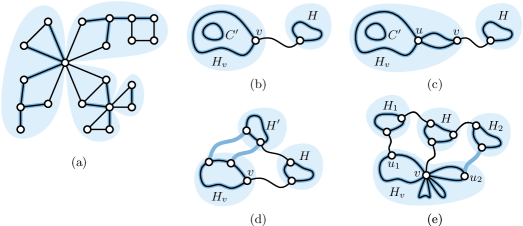
We define to be common connected if and are
connected by a path in ; see
Figure 7a. The split component
is exclusive connected, if it is not common
connected but and are connected by exclusive paths in both
graphs and ; see
Figure 7b. It is
-connected, if and are connected by a path
in but not in ; see
Figure 7c. The term
-connected is defined analogously; see
Figure 7d. Note that being
- or -connected excludes being common or
exclusive connected. Finally, if is neither of the above,
it is union connected; see
Figure 7e.
We say that is an impossible P-node if is a
cycle and one of the split components is -connected, if
is a cycle and one of the split components is
-connected, or if is a cycle
and one of the split components is exclusive connected.
Figure 7: (a–e) A split component that is common connected,
exclusive connected, -connected,
-connected, and union connected, respectively.
(f) The face between two virtual edges that are
-linked (i.e., connected in ).
Lemma 5.
A Sefe instance with an impossible P-node is a no-instance.
Proof.
Let be the split components with respect
to the poles and of the P-node . As is an
impossible P-node, the union-link graph is a cycle.
Thus, at most one split component can be common connected. As
and are the poles of a P-node of the common graph, one of the
split components must be common connected. Thus, exactly one split
component, without loss of generality , is common
connected.
First assume that is an impossible P-node due to the fact that
is a cycle and one of the split components, without loss
of generality is -connected.
Assume the given Sefe instance admits a
Sefe and assume and are embedded
according to this Sefe. As is
-connected
(Figure 7c), the graph
includes a path from to . Clearly, lies in a
single face of . Let be the corresponding face of the
common graph . The boundary of belongs to the expansion
graphs of two different virtual edges and of
; see Figure 7f.
However, and cannot be -linked (as in
Figure 7f), as otherwise
could not be embedded into the face without having a crossing in
. It follows that cannot be a cycle, a
contradiction.
Analogously, if is a cycle and one of the split
components is -connected, we find a path that
is a witness for a pair of adjacent virtual edges that are not
-linked. It remains to consider the case where
is a cycle and is exclusive
connected. In this case, and include paths
and , respectively, connecting and . As they
both belong to the same split component, they have to be embedded in
the same common face of . Thus, there are adjacent virtual
edges that are neither - nor -linked.
Hence, is not a circle.
∎
Due to this lemma, it is sufficient to consider the case that is
not an impossible P-node. We want to show that the different split
components (in the union graph, with respect to the poles and
of ) can be handled independently. However, we have to exclude a
special case to make this true. Let be one of the split
components that is exclusive connected. We say that has
common ends if it contains a common edge incident to or to
. Figure 8 shows an example,
where the following lemma does not hold without excluding exclusive
connected components with common ends.
Figure 8: The union split component includes the expansion
graphs of all three virtual edges , , and
. The edge pairs and
are -linked, thus the exclusive connected split
component cannot be embedded into the faces between
and or between and . Although
and are neither - nor
-linked, cannot be embedded into the face
between and due to its common end. The
component has no common end and can be embedded into
the face between and .
Lemma 6.
Let be a Sefe instance and let be a
non-impossible P-node whose poles are a separating pair with split
components . Assume is the
only common connected split component and none of the exclusive
connected components has common ends. Then admits a
Sefe if and only if admits a Sefe and
together with the common edge admits a Sefe
for .
Proof.
Assume that and (for )
admit simultaneous embeddings. We show how to combine the
simultaneous embeddings of and to a
simultaneous embedding of . The procedure
can then be iteratively applied to the other split components. We
have to distinguish the cases that is union connected,
-connected, -connected, and exclusive
connected (without common ends).
First assume that is union connected.
Figure 9 shows an example
illustrating the proof for this case. As and are the poles
of a P-node, the common graph has a face that is incident
to and to . Let further and be faces of
incident to and , respectively, that are both part
of the union face . Similarly, we choose faces and
in that are incident to and ,
respectively, and that are both part of . Note that might
have several incidences to the face , i.e., when is a
cutvertex in and one of the corresponding blocks is embedded
into . In this case, we choose such that it has
the same incidence to as , i.e., the common
edges appearing in the cyclic order around before and after
are the same as those that appear before and after
. We ensure the same for and . In the
example in Figure 9,
has two incidences to and two incidences to and the chosen
incidence is marked by an angle.
Figure 9: Two split components of the union graph illustrating the
proof of Lemma 6.
Due to the common edge , we can assume that the Sefe of
has and on the outer face. As is not
-connected, we can separate the vertices of
into two subsets and , such that
contains all vertices of the connected component of
containing , while contains all other vertices. We can
then embed the vertices of into and the vertices
of into without changing the embedding of
. In the same way, can be embedded into
and .
As we did not change the embedding of or , the
edge orderings are consistent for all vertices except maybe and
. Moreover, the relative positions between connected components
in is consistent and the same holds for . As
the four faces , , , and belong
to the same common face , the relative positions of components in
with respect to components in are also consistent.
Moreover, all components of lie in the outer face of
with respect to and . Finally, the edge ordering
at is consistent, as all edges incident to in and
are embedded between the same pair of common edges in
. As the same holds for , we obtain a simultaneous
embedding of .
If is -connected, we know that
is not a circle (otherwise, would be impossible). Thus, we
can choose the faces , , and such that
. Then we can embed into this face
without separating it. All remaining arguments work the same as
above. The case that is -connected is
symmetric.
Finally, if is exclusive connected, there is a pair of
virtual edges that are neither - nor
-linked. Thus, we can choose the common face and
the faces , , , and belonging
to such that and . Unfortunately, we cannot always ensure that and
have the same incidence to or ; see
Figure 8. However, the arguments
form the previous cases still ensure that all relative positions and
all cyclic orders except for maybe at and are consistent.
As has no common ends, all common edges incident to
and are contained in and thus the cyclic orders around
these vertices are also consistent.
Note that combining the simultaneous embeddings and
in this way (for all four cases) maintains the properties
that there are faces in , , or that are
incident to both poles and . Thus, we can continue adding
embeddings of all remaining subinstances
in the same way.
∎
Assume we exhaustively applied
Lemma 4,
Lemma 5, and
Lemma 6 to a given instance of
Sefe and let be the resulting instance. Let
and be the poles of a P-node of the common graph such that
are a separating pair in the union graph. By
Lemma 4 we can assume
that does not separate a common cycle. Thus, exactly one
split component has a common -path. By
Lemma 5, we can assume that is a
non-impossible P-node. Thus, we could apply
Lemma 6 if there were split
components without common ends. Hence we obtain the following theorem.
Theorem 3.
Let be an instance of Sefe. In linear time,
we can find equivalent instances such that every union separating
pair has one of the following properties.
•
The vertices and are not the poles of a P-node of a
common block.
•
Every split component has a common edge incident to or to
but only one has a common -path.
Proof.
It remains to prove the claimed running time. The linear running
time for decomposing the instances along its union separating pairs
that separate a common cycle was already shown for
Theorem 2. In
Section 4.3 we extend the
algorithm by Angelini et al. [1] for solving
Sefe if the common graph is biconnected to the case where
we allow exclusive vertices and have so-called union bridge
constrains. It is not hard to see that testing for the
existence of impossible P-nodes can be done using the linear-time
algorithm from Section 4.3.
It remains to decompose the union graph according to
separating pairs that separated according to
Lemma 6. As in the proof of
Theorem 2, we consider the
SPQR-tree of . For
Theorem 2, we had to compute
for every virtual edge, whether its expansion graph included a
common path between its endpoints. Now, we in addition have to know
which expansion graphs are exclusive connected and have common ends.
This can be done analogously to the proof of
Theorem 2.
∎
3.3 Connected Components that are Biconnected
Let be a Sefe instance and let be a connected
component of the common graph that is a cycle; see
Figure 10a. A union bridge of
and with respect to is a connected component of
together with all its attachment vertices on ; see
Figure 10b. Equivalently, the union bridges
are the split components of with respect to the vertices of
excluding the edges of . Similarly, there are
-bridges and -bridges, which
are connected components of and together with their
attachment vertices on , respectively; see
Figure 10c–d. We say that two bridges
and alternate if there are attachments of
and attachments of , such that the order along
is ; see Figure 10e. We have
the following lemma, which basically states that we can handle
different union bridges independently
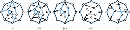
Figure 10: Situation where the connected component of is a
cycle. (a) A simultaneous embedding of with on
the outer face. (b) Removing yields a single connected
component in . Thus, there is only one union bridge.
Its attachment vertices are illustrated as black dots. (c) The
two -bridges. (d) The three -bridges.
Note that different bridges might share attachment vertices.
(e) Two alternating -bridges.
Lemma 7.
Let and be two planar graphs and let be a connected
component of the common graph that is a cycle. Then the
graphs and admit a Sefe where is the boundary
of the outer face if and only if
(i)each union bridge admits a Sefe together with and
(ii)no two -bridges of alternate for .
Proof.
Clearly the conditions are necessary; we prove sufficiency.
Let be the union bridges with respect to , and
let be the
corresponding simultaneous embeddings of together with ,
which exist by condition (i). Note that each union bridge is
connected, and hence all its edges and vertices are embedded on the
same side of . After possibly flipping some of the embeddings,
we may assume that each of them has with the same clockwise
orientation as the outer face.
We now glue to an embedding
of , which is possible by condition (ii). In the same way,
we find an embedding of from .
We claim that is a Sefe of and .
For the consistent edge orderings, observe that any common
vertex with common-degree at least 3 is contained, together with
all neighbors, in some union bridge . The compatibility of the
edge ordering follows since is a Sefe.
Concerning the relative position of a vertex and some common
cycle , we note that the relative positions clearly coincide
in and for . Otherwise is contained in
some union bridge. If is embedded in the interior of in
one of the two embeddings, then it is contained in the same union
bridge as , and the compatibility follows. If this case does
not apply, it is embedded outside of in both embeddings, which
is compatible as well.
∎
We note that this approach fails, when the cycle is not a
connected component of , i.e., when a union bridge contains common
edges incident to an attachment vertex. The reason is that the order
of common edges incident to this attachment vertex is chosen in the
moment one reinserts the union bridges into .
Now consider a connected component of the common graph of a
Sefe instance such that is biconnected. Such a component is
called 2-component. If is a cycle, it is a trivial
2-component. We define the union bridges, and the -
and -bridges of and with respect to as
above. We call an embedding of together with an
assignment of the union bridges to its faces admissible if and
only if, (i) for each union bridge, all attachments are incident to
the face to which it is assigned, and (ii) no two - and
not two -bridges that are assigned to the same face
alternate.
In the following, we try to solve the given Sefe instance
by first finding an admissible embedding of the
2-component . Then we test for every face of whether all union
bridges can be embedded inside the corresponding facial cycle. By
Lemma 7 we know that this is possible if and only
if each union bridge together with the facial cycle admits a
Sefe and no two -bridges (for )
alternate. The latter is ensured by property (ii) of the admissible
embedding of . The former yields simpler Sefe instances
in which the 2-component is represented by a simple cycle. It
remains to show that, if this approach fails, there exists no
Sefe. First note that the properties (i) and (ii) of an
admissible embedding are clearly necessary. Thus, if there is no
admissible embedding of , then there is no Sefe. It
remains to show that it does not depend on the admissible embedding of
one chooses, whether a union bridge together with the facial cycle
of the face it is assigned to admits a Sefe or not. In fact,
the following lemma shows that the facial cycle one gets for a union
bridge is more or less independent from the embedding of , i.e.,
the attachment vertices of the bridge always appear in the same order
along this cycle.
Lemma 8.
Let be a biconnected planar graph and let be a set of
vertices that are incident to a common face in some planar
embedding of . Then the order of in any simple cycle of
containing is unique up to reversal.
Proof.
Consider a planar embedding of where all vertices in
share a face, and let denote the corresponding facial cycle.
Note that is simple since is biconnected. Let be an
arbitrary simple cycle in containing all vertices in .
In , all parts of that are disjoint from are embedded
outside of . Let denote the cycle obtained from
by contracting all maximal paths whose internal vertices do not
belong to to single edges. Observe that and visit
the vertices of in the same order. Consider the graph , which is clearly outerplanar and biconnected. Hence both
and visit the vertices of in the same order (up to
complete reversal). Since was chosen arbitrarily, the claim
follows.
∎
For a union bridge , let denote the cycle consisting of the
attachments of in the ordering of an arbitrary cycle of
containing all the attachments. By
Lemma 8, the cycle is uniquely
defined. Let further denote the graph consisting of the union
bridge and the cycle connecting the attachment vertices of
. We call this graph the union bridge graph of the bridge
. The following lemma formally states our above-mentioned strategy
to decompose a Sefe instance.
Lemma 9.
Let and be two connected planar graphs and let be a
2-component of the common graph . Then the graphs
and admit a Sefe if and only if
(i)admits an admissible embedding, and
(ii)each union bridge graph admits a Sefe.
If a Sefe exists, the embedding of can be chosen as an
arbitrary admissible embedding.
Proof.
Clearly, a Sefe of and defines an embedding of
and a bridge assignment that is admissible. Moreover, it induces a
Sefe of each union bridge graph.
Conversely, assume that admits an admissible embedding and each
union bridge graph admits a Sefe. We obtain a Sefe of
and as follows. Embed with the admissible embedding and
consider a face of this embedding with facial cycle .
Let denote the union bridges that are assigned to
this face, and let
be simultaneous embeddings of the bridge graphs . By
subdividing the cycle , in each of the embeddings, we may
assume that the outer face of each in the
embedding is the facial cycle with the
same orientation in each of them. By Lemma 7,
we can hence combine them to a single Sefe of all union bridges
whose outer face is the cycle . We embed this Sefe into the
face of . Since we can treat the different faces of
independently, applying this step for each face yields a Sefe
of and with the claimed embedding of .
∎
Lemma 9 suggests a simple strategy for reducing
Sefe instances containing non-trivial 2-components. Namely,
take such a component, construct the corresponding union bridge
graphs, where occurs only as a cycle, and find an admissible
embedding of . Finding an admissible embedding for can be done
as follows. To enforce the non-overlapping attachment property,
replace each -bridge of by a
dummy -bridge that consists of a single vertex
that is connected to the attachments of that bridge via edges
in . Similarly, we replace -bridges, which are
connected to attachments via exclusive edges in . We seek a
Sefe of the resulting instance (where the common graph is
biconnected), additionally requiring that dummy bridges belonging to
the same union bridge are embedded in the same face. We also refer to
such an instance as Sefe with union bridge
constraints. A slight modification of the algorithm by Angelini et
al. [1] can decide the existence of such an
embedding in polynomial time. This gives the following lemma.
Lemma 10.
Computing an admissible embedding of a 2-component is equivalent
to solving Sefe with union bridge constraints on an
instance having as common graph. This can be done in polynomial
time.
It then remains to treat the union bridge graphs. Exhaustively
applying Lemma 9 (using
Lemma 10 to find admissible
embeddings) results in a set of Sefe instances where each
2-component is trivial. Note that we could go even further and
decompose along cycles that have more than one union bridge. However,
this is not necessary to obtain the following theorem.
Theorem 4.
Given a Sefe instance, an equivalent set of instances of total
linear size such that each 2-component of these instances is trivial
can be computed in polynomial time.
We can improve the running time in
Theorem 4 to linear. However, it
is quite tedious work, involving a lot of data structures, and results
in a lengthy proof. To not disturb the reading flow too much, the
proof is deferred to its own section (Section 4,
starting on page 4). Here, we only sketch it
very roughly.
We do not apply an iterative process, removing one 2-component after
another (as suggested above), but we decompose the whole instance at
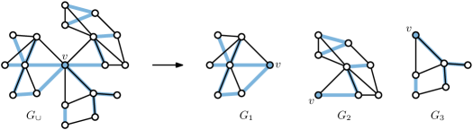
once. For this, we introduce the notion of subbridges. A
subbridge of a graph with respect to components is
a maximal connected subgraph of that does not become disconnected
by removing all vertices of one component ; see
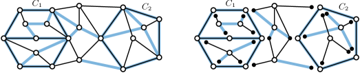
Figure 11.
Figure 11: The instance on the left contains two 2-components
and . The corresponding union subbridges are shown on the
right.
Recall that we have to deal with bridges in two ways. First, each
2-component forms a Sefe instance with its
-bridges, while the union bridges partition these
-bridges (yielding union bridge constraints). Second,
each union bridge yields a union bridge graph, which is a simpler
instance one has to solve. In both cases, one can deal with
subbridges instead of the whole bridges for the following reason. For
the first case, we need the -bridges only to create the
corresponding dummy bridges. Thus, it suffices to know their
attachment vertices. It is readily seen that each bridge of
contains a unique subbridge incident to and that the
attachments of at are exactly the attachments of
at . As this also holds for the union bridges, the union
subbridges already define the correct grouping of the
-subbridges. Concerning the second case, the
Sefe instances that remain after exhaustively applying
Lemma 9 are exactly the union subbridges together
with a set of cycles, one for each incident 2-component. To conclude,
it remains to show that each of the following three steps runs in
linear time.
1.
Compute for each 2-component the number of
incident - and -subbridges, for each such
subbridge its attachments, and the grouping of these subbridges into
union subbridges.
2.
Solve Sefe with union bridge constraints on instances
with biconnected common graph.
3.
Compute for each union subbridge a corresponding instance where each 2-component has been replaced by
a suitable cycle.
For step 1 (Section 4.1), we
contract every 2-component of into a single vertex. The
union subbridges are then basically the split components with respect
to the resulting vertices. The same holds for the - and
-subbridges (using and instead of ).
For step 2 (Section 4.3), we
modify the algorithm due to Angelini et al. [1].
Augmenting it such that it computes admissible embeddings in
polynomial time is straightforward. Achieving linear running time is
quite technical and, like the linear version of the original
algorithm, requires some intricate data structures. For Step 3
(Section 4.2), computing the union subbridges
is easy. To compute a suitable cycle for each incident 2-component
, one can make use of the fact that we already know an admissible
embedding of from step 2.
Theorem 5.
Given a Sefe instance, an equivalent set of instances of total
linear size such that each 2-component of these instances is trivial
can be computed in linear time.
3.4 Special Bridges and Common-Face Constraints
In Section 3.3, we considered the case
that is a 2-component of the common graph . We called the
split components with respect to the vertices of bridges
(excluding edges in ). Clearly, this definition extends to the
case where is an arbitrary connected component. However, the
decomposition into smaller instances does not extend to this more
general case as for example Lemma 8 fails
for non-biconnected graphs. Nonetheless, we are able to eliminate
some special types of bridges in exchange for so-called common-face
constraints. The reduction we describe in this section is thus in a
sense weaker than the previous reductions as we reduce a given
Sefe instance to a set of equivalent instances with
common-face constraints. Many algorithmic approaches allow an easy
integration of additional common-face constraints (see
Section 5.3) and hence the more simple
instances resulting from the reduction outweigh the disadvantages
caused by the additional constraints (see
Section 5.4).
Let be an instance of Sefe with common graph
and let be a family of sets of common
vertices. A given Sefe satisfies the common-face
constraints if and only if has a face incident to
all vertices in for every . The common-face
constraints are block-local if for every all vertices in belong to the same block of .
Similarly, we say that a union bridge is block-local if all
attachment vertices of belong to the same block of . Let
be the -bridges (for ) belonging to . We say that is exclusively
one-attached if has only a single attachment vertex for
.
Let be a block-local union bridge of the common connected
component . Then the attachment vertices of appear in the same
order in every cycle of (Lemma 8).
Thus, we can define the union bridge graph of as in
Section 3.3. Consider the
Sefe instance obtained from by
removing the union bridge (the attachment vertices are not
removed). It follows from Section 3.3
that admits a Sefe if and only if the union
bridge graph admits a Sefe, and admits a
Sefe with an assignment of to one of its faces such
(i)all attachment vertices of are incident to , and
(ii)for , no -bridge in alternates
with another -bridge in .
If is not only block-local but also exclusive one-attached, the
latter requirement is trivially satisfied (a -bridge that
has only a single attachment vertex cannot alternate). Thus, it
remains to test whether admits a Sefe and
admits a Sefe with block-local common-face constraints. We
obtain the following theorem. The linear running time can be shown as
in Section 4.
Theorem 6.
Given a Sefe instance, an equivalent set of instances with
block-local common-face constraints of total linear size can be
computed in linear time such that each instances satisfies the
following property. No union bridge of a common connected component
that is not a cycle is block-local and exclusively one-attached.
4 Preprocessing 2-Components in Linear Time
As promised in the end of Section 3.3,
we prove in this section that the decomposition of a Sefe
instance into equivalent instances where every 2-component is a cycle
can be done in liner time. Readers who want to skip this section can
continue with Section 5 on
page 5.
4.1 Computing the Sefe-Instances with Union Bridge
Constraints
We first consider a slightly more general setting. Let be a
graph and let be disjoint connected subgraphs of .
We are interested in computing the number of bridges of each connected
component together with the attachments to . We show that
this can be done in time (even if is non-planar),
where and . Instead of computing directly the
bridges and their attachments, our goal is rather to label each
edge that is incident to a vertex of some but does not
belong to any of the itself, by the bridge of that
contains . Observe that, if each such incident edge has been
labeled, the information about the number of -bridges and their
attachments can easily be extracted by scanning all incidences of
vertices of for . This scanning process can
clearly be performed in total time. In the following, we
thus focus on computing this incidence labeling. Note that, since we
are only interested in the attachments of bridges, it suffices to
consider the corresponding subbridges as they have the same attachment
sets.
Recall that a subbridge is a maximal connected subgraph of for
which none of the is a separator. Note the high similarity of
the definition of subbridges and the blocks of a graph, which are
maximal connected subgraphs for which no single vertex is a separator.
As with the blocks of a graph, it is readily seen that each edge
of that is not contained in one of the is contained in
exactly one subbridge of . We exploit this similarity further and
define the component-subbridge tree of with respect
to as the graph that contains one vertex for
each component and one vertex for each subbridge .
Two vertices and are connected by an edge if and only if
the subbridge is incident to the component . Note that,
indeed, the component-subbridge tree is a tree. Once the
component-subbridge tree has been computed, we can label each edge
of with the subbridge containing
it.
Lemma 11.
The component-subbridge tree of a graph with respect to disjoint
connected subgraphs can be computed in linear time.
Proof.
First, contract each component to a single vertex ; call
the resulting graph . Note that, in , the subbridges are
exactly the maximal connected subgraphs for which none of the
vertices is a separator. We compute the component-subbridge
tree in three steps. First, compute the block-cutvertex tree
of . Second, for each cutvertex that does not correspond to
one of the , remove and merge its incident blocks into the
same subbridge. Finally, create for each component that has
only one bridge a corresponding vertex and attach it as a leaf
to the unique subbridge incident to . Clearly, each of the
steps can be performed in time.
∎
As argued above, Lemma 11 can be used
to label in linear time the incident edges of the
components by their corresponding bridges. For step 1
of our reduction, we take as the 2-components of a
Sefe instance . We then use the above approach to
label the attachment incidences of the -, -,
and the union bridges of . From this we can create the
dummy bridges for each 2-component together with the union
bridge constraints in time linear in the sum of degrees of vertices
in . By the arguments for
Lemma 10, the resulting instance
admits a Sefe if and only if has an admissible
embedding. Since the are disjoint, it follows that the
construction of all instances can be done in linear time. This
finishes step 1.
4.2 Constructing the Subbridge Instances
Let us assume that each 2-component has an admissible embedding, which
is found using the linear-time algorithm described in
Section 4.3. Otherwise a
Sefe of the original graph does not exist. In the final step
of our reduction, we substitute, in each subbridge, the incident
2-components by a cycle. This results in a set of Sefe
instances—one for each subbridge—that all admit a solution if and
only if the original instance admits a solution. They can hence be
handled completely independently. To efficiently extract all
instances, we process the 2-components independently and replace each
one by a cycle in their incident subbridges. The time to process a
single 2-component with all its incident subbridges is linear in the
size of the 2-component plus the number of attachments of these
subbridges in the respective 2-component. It then immediately follows
that processing all 2-components in this way takes linear time.
Consider a fixed 2-component with an admissible embedding as
computed in step 2 of the reduction. Consider a fixed face
together with the subbridges that are embedded in that face. For each
bridge embedded in , we construct a list of attachments .
We traverse the facial cycle of . At each vertex, we check the
edges embedded inside this face and append the vertex to the list of
each subbridge for which it is an attachment. Afterwards, we traverse
for each subbridge its list of attachments and replace by a cycle
that visits the attachments in the order of the attachment list. The
time is clearly proportional to the size of and the attachments of
the subbridges embedded in . Hence processing all faces of all
components in this way takes linear time and yields the claimed
result. This implements step 3 in linear time.
4.3 Simultaneous Embedding with Union Bridge Constraints
In this section, we show how to solve Sefe with union bridge
constraints in linear time if the common graph is biconnected. Our
algorithm is based on the algorithm by Angelini et
al. [1]. Note that our extension to this algorithm
is twofold. We allow bridges with an arbitrary number of attachment
vertices. The original algorithm allows only two attachments per
-bridge (i.e., each bridge is a single exclusive edge).
Moreover, we have to deal with union bridge constraints. To avoid
some special cases and simplify the description, we sometimes deviate
from the notation used by Angelini et al. Our focus lies on a
linear-time implementation, the correctness of our approach directly
follows from the correctness of the algorithm by Angelini et al.
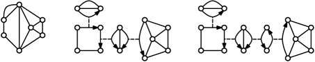
Figure 12: A graph (left) together with its SPQR-tree (middle). The
Q-nodes are omitted to improve readability. The augmented
SPQR-tree (right) contains an additional S-node whose skeleton is
a cycle of length 2.
Let be the biconnected common graph. We consider the (unrooted)
augmented SPQR-tree of , which is defined as follows;
see Figure 12. Let be the SPQR-tree
of and let and be two adjacent nodes in such
that each of them is a P- or an R-node. We basically insert a new
S-node between and whose skeleton is a cycle of
length 2 (i.e., a pair of parallel virtual edges). More precisely,
let and be the virtual edges
in and , respectively, that correspond to each other.
We subdivide the edge in ; let be the new
subdivision vertex. The skeleton contains the vertices
and with two virtual edges and between
them corresponding to in and in
, respectively. Applying this augmentation for every
pair of adjacent nodes that are P- or R-nodes gives the augmented
SPQR-tree . Note that P- and R-nodes in have only S- and
Q-nodes as neighbors. Moreover, no two S-nodes are adjacent.
Consider a bridge and let be a node of . A virtual edge
in is an attachment of if its expansion
graph contains an attachment vertex of . We say that is
important for if it has at least two distinct attachments
among the vertices and virtual edges of that are not two
adjacent vertices in . It is clearly necessary, that
admits an embedding such that for every union bridge
the attachments in are incident to a common face. An
embedding having this property is called compatible. This
leads to the following first step of the algorithm.
Step 1 (Compatible embeddings).
For every P- and R-node , compute the important union bridges
with their attachments. If is an R-node, check whether the
unique (up to flip) embedding is compatible. If
is a P-node check whether it admits a compatible embedding and fix
such an embedding (up to flip).
If Step 1 fails, the instance does not admit a
Sefe. Note that the skeleton of a P-node might admit several
compatible embeddings. However, fixing an arbitrary compatible
embedding up to flip does not make a solvable Sefe instance
unsolvable [1]. Thus, after Step 1, we
can assume that the embedding of every skeleton is fixed and it
remains to decide for each skeleton whether its embedding should be
flipped or not. We call the embedding fixed for a skeleton its
reference embedding.
For every P- and R-node let be a binary decision
variable with the following interpretation. The skeleton
is embedded according to its reference embedding and according to the
flipped reference embedding if and ,
respectively. By considering the S-nodes of the augmented SPQR-tree,
one can derive necessary conditions for these variables that form an
instance of 2-Sat (actually, we only get equations and
inequalities, which is a special case of 2-Sat).
Let be an S-node. We assume the edges in to be
oriented such that is a directed cycle. Thus, we can use
the terms left face and right face to distinguish the faces of
. Let be a bridge that is important for . We
can either embed into the left or into the right face of
. We define the binary variable with the
interpretation that is embedded into the right face and into the
left face of if and ,
respectively.
Figure 13: An S-node with a bridge having as right-sided
attachment. The virtual edges are illustrated as gray regions
with their expansion graph inside.
Assume that the virtual edge (oriented from to ) in
is an attachment of , i.e., an attachment vertex of lies in the expansion graph of . Let
be the neighbor of corresponding to and let
be the twin of in (also oriented from
to ); see Figure 13. Clearly, is
also important for as contains an attachment vertex of
while the attachment vertex is not contained in . In
Step 1 we ensured that is embedded such that
(or the virtual edge containing ) shares a face with .
If this face lies to the left of in , we say that
is an attachment on the right side of in
(as in the example in
Figure 13). Otherwise, if this faces lies
to the right of , we say that is an attachment on the
left side of . For a bridge with attachment vertex
we also say that the attachment is right-sided and
left-sided if lies on the right and left side of ,
respectively.
Assume has an attachment on the right side of the virtual edge
in the skeleton (as in
Figure 13). Assume further that the
skeleton of the corresponding neighbor is not flipped,
i.e., . Then must be embedded into the face to the
right of the cycle , i.e., . Conversely, if
the embedding of is flipped, i.e., , then
must lie in the left face of , i.e., .
This necessary condition is equivalent to the equation . Similarly, if has an attachment on the left side of
, we obtain the inequality . We call
the resulting set of equations and inequalities the consistency
constraints of the bride in . This leads to the second
step of the algorithm.
Step 2 (Consistency constraints).
For every S-node compute the important -bridges
(for ) and union bridges together with their
attachments. For attachments in virtual edges also compute whether
they are left- or right-sided. Then add the consistency constraints
of these bridges in to a global 2-Sat formula.
The consistency constraints are necessary but not sufficient as they
do not ensure that no two alternating bridges of the same type are
embedded into the same face. Consider an S-node with two
important bridges and . Assume these two bridges alternate
(i.e., they have alternating attachments in the cycle ).
Embedding and on the same side of yields a
crossing between an edge in and an edge in . Thus, if and
are both - or both -bridges, then they
must be embedded to different side of . In this case, we
obtain the inequality . This inequality is
called planarity constraint.
Step 3 (Planarity constraints).
For every S-node compute the pairs of important
-bridges that alternate in . Do the same
for -bridges. For each such pair add the planarity
constraint to the global 2-Sat formula.
Finally, we have to embed -bridges belonging to the same
union bridge into the same face. Let be an -bridge
and let be the union bridge it belongs to. The
union-bridge constraint of in is the equations
.
Step 4 (Union-bridge constraints).
For every S-node , add the union-bridge constraint of each
important -bridge to the global 2-Sat formula.
After Steps 2–4, the global 2-Sat
formula is solved in linear time [2]. The solution
determines for every P- and every R-node , whether the reference
embedding of should be flipped or not, which completely
fixes the embedding of the common graph . Of course, there might
be different solutions of the 2-Sat formula, yielding
different embeddings. However, if one of these solutions yields a
Sefe, then any of the solutions does [1].
Thus, one can simply take one solution and check whether it yields a
Sefe (with union bridge constraints) or not.
Step 5 (Final step).
Test whether the given instance admits a Sefe with union
bridge constraints assuming that the embedding of the common graph
is fixed.
It remains to implement Steps 1–5 in linear
time, which is done in the following. We first note that there are
too many important bridges to be able to compute them in linear time
(as required in Step 1 and Step 2). However,
similar to Angelini et al. [1], we can show that
many important bridges can be omitted without loosing the correctness
of the algorithm, which leads to a linear-time implementation.
4.3.1 Too Many Bridges are Important
We start with the observation that computing all important union
bridges for every P- and R-node of the SPQR-tree is actually a bad
idea, as there may be bridges each being important in
nodes. Thus, explicitly computing all of them would
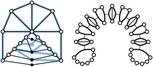
require time. Consider the graph in
Figure 14 whose SPQR-tree
(without Q-nodes) is a path. Let be one of the
P-nodes (note that has two virtual edges and one normal
edge) and let be one of the bridges shown in
Figure 14. Clearly, the
expansion graphs of both virtual edges of contain at
least one attachment vertex of . Thus, is important for
and has the two virtual edges of as attachments. As
this may hold for a linear number of bridges, we get the above
observation.
Figure 14: A graph with many bridges (left) each of which being
important for every node of the SPQR-tree (right).
To resolve this issue, note that from the perspective of (in the
above example), all bridges look the same in the sense that they have
the same set of attachments. Intuitively, they thus lead to similar
constraints and it seems to suffices to know only one of these
bridges. In the following, we first show that omitting some of the
bridges is indeed safe in the sense that the algorithm remains
correct. Then we show how to compute the remaining bridges
efficiently.
4.3.2 Omitting Some Important Bridges
In this section we show how to change the algorithm described above
(Steps 1–5) slightly without changing its
correctness. We say it is safe to do something if doing it
does preserve the correctness of the algorithm. In particular, we
show that it is safe to omit some of the important bridges. In the
subsequent sections we then show that the remaining important bridges
can be computed efficiently leading to an efficient implementation of
all five steps.
Let be the common graph and let be its SPQR-tree.
Let be an inner node of and let be a bridge
that is important for with attachments in
(recall that each of the is either a vertex or a
virtual edge of ). We call an attachment (with ) superfluous, if is a vertex in
such that has another attachment that is a
virtual edge incident to the vertex ; see
Figure 15a. The following lemma shows
that the term “superfluous” is justified.
Figure 15: (a) The bridge has five attachments .
Attachments and are superfluous due to and
, respectively. (b) The bridges and alternate only
due to the superfluous attachment of . However, the
consistency constraints already synchronize and as they
have as common attachment.
Lemma 12.
Omitting superfluous attachments is safe.
Proof.
There are two situation in which missing superfluous attachments
might play a role. First, when we check a P- or R-node skeleton for
a compatible embedding (Step 1). Second, when we add the
planarity constraints for alternating -bridges
(Step 3). Let be the superfluous attachment of
and let be a virtual edge incident to that is also an
attachment of in . Concerning compatible
embeddings, we have to make sure that admits an
embedding where all attachments of are incident to a common
face. Clearly, is incident to both faces the virtual edge
is incident to. Thus, omitting the attachment does not
change anything.
Concerning the planarity constraints, we have to consider the case
that alternates with another bridge only due to the
attachment in . This can only happen if has as
attachment; see Figure 15b. However,
then the consistency constraints (Step 2) either forces
and into different faces (if their attachment in
lies on different sides of ) and everything is fine, or they
force and to lie in the same face. In the latter case, the
instance is clearly not solvable, which will be found out in
Step 5.
∎
In the following we always omit superfluous attachments even when we
do not mention it explicitly. Note that this retroactively changes
the definition of important bridges slightly, i.e., a bridge is
important for a node if has at least two (non-superfluous)
attachments in .
To show that we can omit sufficiently many important bridges to get a
linear running time, we have to root the SPQR-tree . More
precisely, we choose an arbitrary Q-node as the root of .
We categorize the important bridges in different types of bridges
depending on their attachments. To this end, we first define
different types of attachments. Let be a node of the (rooted)
SPQR-tree and let be an important bridge of with attachments
. Recall that an attachment is either a vertex of
a virtual edge of . If is a pole of ,
we call it a pole attachment. If is the parent edge of
, we call it parent attachment. All other
attachments are called child attachments.
We say that the important bridge is a regular bridge of
if has at least two child attachments. If has only a
single child attachment, it has either a parent attachment or one or
two pole attachments (note that pole attachments are superfluous in
the presence of a parent attachment). We call parent
bridge and pole bridge in the former and latter case,
respectively. Note that must have at least one child attachment
as it otherwise cannot be important.
As shown before, we cannot hope to compute all important bridges
efficiently as there may be too many of them. Thus, we show in the
following that omitting some important bridges is safe.
Lemma 13.
Let be a parent bridge whose child attachment is a virtual
edge. Omitting another parent bridge or a pole bridge with child
attachment (while keeping ) is safe.
Proof.
Let be an other important bridge of and let be the
child attachment of and . Let be the parent edge of
. In Step 1, the bridge forces the
embedding of to have and on a common face.
If is a parent bridge, it requires the same (and thus no
additional) condition for the embedding of . If is
a pole bridge, it requires one of the poles (or both of them) to be
incident to a common face with . However, this is clearly the
case if the parent edge (which is incident to both poles)
shares a face with . Hence, omitting does not change
anything in Step 1.
We cannot argue separately for Steps 2–4 as
they all contribute to the same global 2-Sat formula. We
call the 2-Sat formula we get when omitting
new. The formula we get when not omitting is called
original. The straightforward way to prove that omitting
is safe would be to show that the new and the original
2-Sat formulae are equivalent in the sense that they have
the same solutions. However, this is not true as omitting can
make the 2-Sat formula solvable whereas it was unsolvable
before.
Assume the original 2-Sat formula is not solvable. Then
the given instance does not admit a Sefe with union bridge
constraints. In this case, Step 5 will never succeed no
matter what we do in the steps before. Thus, we only have to argue
for the case that the original 2-Sat formula is solvable.
In this case, the only thing that can go wrong is that the new
2-Sat formula admits a solution that is not a solution in
the original formula. This solution could then result in an
embedding of the common graph that does not admit a
Sefe, whereas all solutions of the original 2-Sat
formula lead to a Sefe.
To get a handle on this, we consider the conflict graph of a
2-Sat formula. First note that the formula we obtain is
special in the sense that each constraint is either an equation or
an inequality. We define the conflict graph to have a vertex for
each variable and an edge connecting two vertices if there is an
(in-)equality constraint between the corresponding variables.
Recall that the 2-Sat formula has a variable for
every P- or R-node indicating whether the embedding of
has to be flipped or not. In the following we show
that two such variables and that are in the same
connected component of the conflict graph of the original
2-Sat formula are also in the same connected component with
respect to the new formula. This shows that every embedding
resulting from a solution of the new formula also yields a solution
of the original formula (assuming that the original formula has a
solution at all).
First note that omitting an important bridge in an S-node
has the effect that the vertex corresponding to the variable
is deleted in the conflict graph (for convenience we
also denote the vertex by ). Recall that the variable
represents the decision of whether is embedded
into the left or the right face of . We show that
is dominated by in the sense that every
neighbor of is also connected to by a path
not containing . Thus, removing does not
change the connected components of the conflict graph.
Consider the consistency constraints of (Step 2).
Let be an attachment of . If is a vertex in
, we do not get a consistency constraint there. If
is a virtual edge, it corresponds to a neighbor of and
we get the constraint or . But then has also as attachment and thus we
also have one of the two constraints or .
For the planarity constraints (Step 3), first assume that
is a parent bridge. Then alternates with another bridge
if and only if alternates with . Thus, if we have
the constraint we also have the constraint
. If is a pole bridge, there might be a
bridge alternating with (yielding the constraint ), whereas and do not alternate. However,
this can only happen if has the parent edge of
as attachment. Let be the neighbor of
corresponding to (i.e., the parent of ). From
Step 2 we then have the consistency constraint between
and and also one between and
( is a parent bridge). Thus, the conflict graph
includes the path , which still exists
after removing .
Finally, if is the union-bridge including , we loose the
union-bridge constraint (Step 4) by omitting . Note that the attachments of
are a subset of the attachments of . Thus, has the child
attachment (which is a virtual edge). Let be the
neighbor of corresponding to . Then we have a consistency
constraint connecting with . Moreover,
is also connected to as is an attachment of
. This yields a connection from to .
∎
This lemma gives rise to the following definition. Let be a pole
bridge of with child attachment that is a virtual edge in
. Let further be a parent bridge of with child
attachment . We say that is dominated by . If
is a parent bridge of with child attachment instead, we say
that and are equivalent. Note that being equivalent
is clearly an equivalence relation. Lemma 13
shows that we can omit dominated pole bridges and all but one parent
bridge for each equivalence class.
4.3.3 Computing the Remaining Important Bridges
In this section we show that all bridges that are not omitted due to
Lemma 13 can be computed in linear time.
Actually, we compute slightly more information, which we need in some
intermediate steps. We for example never omit a parent bridge in
if is regular in the parent of . We call such a bridge
semi-regular in .
Moreover, consider an important bridge of and let be an
attachment of in that is a virtual edge. A vertex
of that is not incident to in is a
representative of the attachment if is an attachment
vertex of and included in the expansion graph of . If the
attachment is a vertex of , we say that is its own
representative. Note that every attachment of has at least one
representative vertex. When we compute the important bridges of a
node , we also compute their attachments in together with
at least one representative for each attachment. Before we actually
compute bridges, we provide some general tools.
Lemma 14.
After linear preprocessing time, the pole and parent attachments of
a bridge in a given node together with a representative of each
attachment can be computed in constant time.
Proof.
We first do some preprocessing. We define the
SPQR-vertex-tree to be the tree obtained from
the SPQR-tree by removing its Q-nodes and attaching every vertex
of as a leaf to the highest node that contains in its
skeleton. Note that this is the unique node that contains in
its skeleton but not as pole.
For a non-pole vertex in a skeleton , we say that
the leaf (which is a child of ) corresponds to . Note
that this makes sure that every child attachment in
corresponds to a child of in .
Assume the vertices of (i.e., the leaves of ) to be
numbered according to a DFS-ordering (which we get in time).
We start by sorting the attachment vertices of each bridge according
to this DFS-ordering. For all bridges together,
this can be done in time as
follows. To simplify the notation, we identify every
bridge with its set of attachment vertices. First, sort all
pairs with (i.e., basically the disjoint
union of the ) using bucket sort with buckets
(for each vertex , one bucket containing all pairs ).
It then suffices to iterate over all these sorted pairs to extract
the sets sorted according to this DFS-ordering.
For a node of , the leaves that are descendents of this
node appear consecutively in the DFS-ordering. By going bottom-up
in , we can compute for every node the leaf with
the smallest and the leaf with the largest number among the
descendents of . Thus, given a vertex of , we can
decide in constant time whether is a descendent of .
Now we answer the queries. Let be a bridge that is important in
a node . If the vertex with the smallest and the vertex with
the largest number in (which we can find in constant time as
is sorted) are both descendents of , all attachment vertices of
are descendents of . In this case has neither a pole
nor a parent attachment in . Otherwise, by looking at the
first two and the last two elements in we can distinguish the
following two cases.
(i)There is an attachment vertex that is not a descendent of
and not a pole of . Then the parent edge of
is an attachment of in and is a
representative for this attachment. If also has pole
attachments in , they are superfluous and we can
ignore them by Lemma 12.
(ii)There is no such vertex . Then all attachment vertices in
are descendents of except for maybe the two poles. In
this case, the poles of that are attachments of
are among the first or last two vertices in and thus we find
all pole attachments of in .
This concludes the proof.
∎
Lemma 15.
The regular bridges and their attachments together with a
representative for each attachment can be computed in linear time.
Proof.
Let be the SPQR-vertex-tree of and assume again
that the vertices in every bridge are sorted according to a
DFS-order of the leaves in . We first show how to
compute all nodes in which a given bridge is regular in
time. Note that this implicitly shows that has
only regular vertices.
The lowest common ancestor (LCA) of two vertices and
is the highest node on the path between and . We denote it
by . Clearly, the vertices and are descendents
of different children of . Thus, if has the
attachment vertices and , then has two different child
attachments in with representatives and . Thus,
is active. Conversely, if is regular in a node
, it has two different child attachments. Let and be
representatives of these two attachments. Clearly, and are
descendents of different children of and thus holds. Hence, the nodes in which is regular are exactly
the LCAs of pairs of attachment vertices in .
To see that it is not necessary to consider all pairs of vertices in
, let , , and with (according to the
DFS-ordering) be contained in . Then
or holds for the following reason. If
, then , , and are
descendants of three different children of . Thus, also holds. Otherwise, assume is a
descendant of . Thus, from the perspective of
, the vertices and and the node are descendants
of the same child whereas is the descendant of a different
child. Thus . Hence, to compute
all nodes in which is regular, it suffices to compute the LCA
for pairs of attachment vertices in that are consecutive (with
respect to the ordering we computed before). As the LCA can be
computed in constant time after preprocessing
time [14], this gives us all regular bridges of all
nodes of the SPQR-tree in overall time.
Given a node and a regular bridge of , we are still
lacking the attachments of in . We can get the
parent and pole attachments using
Lemma 14. Consider a child
attachment of in . Note that the attachment
vertices of that are descendants of are consecutive with
respect to the DFS-order. When choosing the first or last of these
vertices, we get an attachment vertex in with the following
properties: is a descendent of the child of that
corresponds to and either for the predecessor
of in (ordered according to the DFS-order) or for the successor of . Thus, we actually already
know a representative for every child attachment of in
. To find for an attachment vertex (the
representative) the corresponding attachment in , we
need to find the child of that has the leaf as a
descendant. This can be done for all active bridges simultaneously
by processing bottom-up while maintaining a union-find
data structure. As the sequence of union operations is known in
advance, each union and find operation takes amortized
time [10]. Thus, it takes time in total.
∎
Lemma 16.
The semi-regular bridges and their attachments together with a
representative for each attachment can be computed in linear time.
Proof.
By Lemma 15, we know for every node all
the bridges that are regular in . We can assume that the
regular bridges of a are stored as a list that is sorted
according to an arbitrarily chosen order of the bridges (we just
have to process the bridges in this order in the proof of
Lemma 15). Moreover, we know all the
attachments of in together with a representative
for each attachment.
Let be a child attachment of in with
representative . Let be the child of corresponding
to . If is a leaf, it actually must be the vertex and
there is nothing to do. Otherwise, is a descendent of
and thus has a child attachment in . Moreover, it also
has a parent attachment in as it otherwise would not be
regular in the parent of . Thus, is either regular
or a parent bridge (and hence semi-regular) in .
By processing all regular bridges of like that, we can build
for (and all other children of ) a list of bridges that
contains all semi-regular bridges and additionally some regular
bridges. Note that building up this list takes constant time for
each attachment of regular bridges. As we computed those
attachments in linear time, there cannot be more than that many
attachments.
To get rid of the bridges that are actually regular and not
semi-regular, note that we can assume the list of semi-regular and
regular bridges to be sorted (according to the arbitrary order of
bridges we chose before). Thus, we can simply process this list and
the list of regular bridges of (which we computed using
Lemma 15) simultaneously and throw out all
those that appear in both lists. This leaves us with a list of
semi-regular bridges for every node. In addition to that, we know
an attachment vertex for every semi-regular bridge that is a
representative of the child-attachment of that bridge. Thus, we
also get the actual attachments in in linear time
using one bottom-up traversal as in the proof of
Lemma 15. Moreover, we get the parent
attachments using Lemma 14.
∎
Lemma 17.
The parent and pole bridges and their attachments together with a
representative for each attachment can be computed in linear time
when omitting dominated pole bridges and all but one parent bridge
of each equivalent classes.
Proof.
Let be the SPQR-vertex-tree of the common graph .
We now process bottom-up computing a list of bridges
for each node . This list will contain all bridges that
potentially are parent or pole bridges in and we denote it by
. More precisely, if a bridge has an attachment
vertex that is a descendent of and other attachment vertices
that are not descendents of , then is contained in
. As we do not have the time to tidy up properly,
can also contain bridges whose attachment vertices are
all descendents of .
We start with the leaves of , which are vertices of .
Let be such a leaf. Then is the list of all bridges
having as attachment. By initializing with the empty
list and then processing all bridges once, we can compute
for all vertices in time. Now
consider an inner node . We basically obtain the list
by concatenating the lists of all children. But before
concatenation we (partially) process these lists separately.
While processing (and the lists computed for the children of
) we want to answer for a given bridge the following
queries in constant time. First, is regular in ? Second,
have we seen already while processing ? This can be done
using timestamps. Assume we have one global array with an entry for
each bridge. Before processing we increment a global
timestamp and write this timestamp into the fields of the array
corresponding to bridges that are regular in . While
processing , we can then check in constant time whether the
current timestamp is set for a given bridge and thus whether
is regular. Setting up this array takes time linear in the number
of regular bridges of and thus we have an overall linear
overhead. We can handle the second query in constant time,
analogously.
Now let be the node we currently process, let be a
child of and assume that is already computed. We
process the list ; let be the current bridge. By
Lemma 14 we can check in constant
time whether has pole or parent attachments in . If not,
all attachment vertices of are descendents of and we
remove form the list as cannot be a parent or
pole in or in any ancestor of .
Otherwise, has a parent or a pole attachment in . We first
check (in constant time) whether is regular in . Assume it
is regular and we see the first time since processing
(which we can also check in constant time as mentioned above). Then
we simply skip and continue processing . If is
regular in and occurred before while processing , it
would be contained twice in the list when concatenating
the lists of all children of . Thus we can remove this
occurrence of from . Afterwards, we continue
processing the remaining bridges in .
Now assume that is not regular. Then is either a parent or
a pole bridge. If is a parent bridge, we store it as a parent
bridge of . Note that we also know the attachments of in
(the parent edge and the attachment corresponding to
the child ) and a representative for each of these
attachments. Afterwards, we stop processing and
continue with another child of . By stopping after processing
, we might miss a bridge in that is also a pole
or parent bridge of . However, the child attachment of
would be the attachment corresponding to and thus is in
the same equivalence class as (if is a parent bridge) or
is dominated by (if is a pole bridge). In both cases
we can omit .
Finally, consider the case that is a pole bridge in . We
save together with its attachments in (and their
representatives) as pole bridge of . Then we remove from
and continue processing . Removing
from has the effect that does not occur when
processing an ancestors of . Thus, we have to show that is
not a pole or parent bridge in one of these ancestors. Consider an
ancestor of . Then either all attachment vertices of
are descendents of and is neither pole nor parent
bridge for . Otherwise, the only attachment vertex of
that is not a descendent of is (without loss of
generality). However, the virtual edge in containing
all attachment vertices of is then incident to and thus the
attachment is superfluous. Hence, we can omit the bridge in
by Lemma 12.
It remains to show that the above procedure runs in linear time.
First note that we add elements to lists only in the
leaves of . As we add each bridge to exactly
such bridges, the total size of these lists is linear. Assume we
are processing a list and let be a bridge we delete
after processing it. Then we can ignore the (constant) running time
for processing , as we have only linearly many such deletion
operations. Otherwise, is a regular bridge that we see the
first time or it is a parent bridge. The former case happens only
as many times as there are regular bridges of (which is
overall linear). The latter case happens at most once for each
child of as we stop processing afterwards.
Hence, the overall running time is linear.
∎
Recall that Step 1 consist of computing the important
union bridges for P- and R-nodes. For every P- and R-node we
then have to test whether admits a compatible
embedding, i.e., whether can be embedded such that the
attachments of each important bridge of share a face.
For each node , we compute the regular and semi-regular bridges
using Lemma 15 and
Lemma 16, respectively. We moreover
compute some of the pole and parent bridges using
Lemma 14. In this way we of
course miss some important bridges but we know by
Lemma 13 that it is safe to do so. Thus, we
can focus on computing compatible embeddings.
Let be a node of the SPQR-tree and assume that is a
P-node. Each of the two vertices and in is
incident to every face. If an important bridge has or
as attachment, this attachment does not constrain the embedding of
(it shares a face with all other attachments of if
and only if all other attachments share a face). Thus, we can
assume that only the virtual edges of are attachments.
If has three (or more) attachments in , it is
impossible to find a compatible embedding as every face of
is incident to only two virtual edges. It remains to
deal with the case where every bridge has two virtual edges as
attachment. We build the conflict graph with one vertex
for every virtual edge and an edge between two such vertices
and if and only if there is a bridge with
attachments and . It is not hard to see that
admits a compatible embedding if and only if this
conflict graph has maximum degree 2 and either contains no cycle or
is a Hamiltonian cycle.
If is an R-node, its skeleton is triconnected and therefore
has a fixed planar embedding. To test whether the embedding of
is compatible, we need to check for every bridge ,
whether there is a face incident to all its attachments. We
consider the graph obtained from by
subdividing every edge and inserting a vertex into every face that
is connected to all incident vertices. We denote the new vertex
created by subdividing the virtual edge by and the
new vertex inserted into the face by . For a vertex
that already existed in we also write . For a
bridge with attachments , we need to test
whether there is a face such that for every pair and
the path is contained in .
To make sure that all paths of length 2 between and
include a vertex corresponding to a face , we
subdivide every edge twice except for those edges incident to a
vertex corresponding to a face.
As is planar, we can use the data structure by Kowalik
and Kurowski [16] that can be computed in linear
time and supports shortest path queries for constant distance in
constant time. More precisely, for any constant , there exists a
data structure that can test in whether a pair of vertices is
connected by a path of length . If so, a shortest path is
returned. We first rule out some easy cases.
If there is an attachment that is a virtual edge in
, the vertex has only four neighbors in
. Thus, we get the two faces incident to in
constant time and can check in time whether one of them is
incident to every attachment of . We thus assume that all
attachments are vertices. If one of these vertices is adjacent to
three or more others, there cannot be a compatible embedding. Thus,
we either find (in time) a pair of non-adjacent attachments
and or there are only two or three pairwise adjacent
attachments. As the latter case is easy, we can assume that we have
non-adjacent attachments and . As is
triconnected, and are incident to at most one common
face . Thus, there is only one path of
length 2 from to in , which gives us in
constant time. Then it remains to check whether all other
attachments are incident to , which takes time. Doing
this for every bridge yields a linear-time algorithm testing whether
an R-node skeleton admits a compatible embedding.
∎
Recall that Step 2 consist of three parts. First we have
to compute the important -bridges of S-nodes together
with their attachments. For each attachment we then have to test
whether it is left- or right-sided. Finally, we have to add the
consistency constraints.
As for Step 1, we use Lemma 15,
Lemma 16, and
Lemma 17 to compute all important
-bridges together with their attachments. We actually
compute these important bridges not only for the S-nodes but also
for P- and R-nodes. We use this additional information to compute
which attachments are left- and which are right-sided.
Note that the final step of adding the consistency constraints to a
global 2-Sat formula is trivial. Thus, it remains to show
that we can compute for every attachment whether it is left- or
right-sided.
Let be a node of the SPQR-tree . We iterate over
all important bridges of (except those we omitted). For every
bridge we iterate over all attachments in and for every
virtual edge among those attachments, we append to the
list . Afterwards, contains all
important (but not omitted) bridges of that have as
attachment. Note that we can assume that the bridges in
are sorted according to an arbitrary but fixed
order of the bridges.
Let be an S-node with virtual edge in .
Let further be the neighboring P- or R-node corresponding to
and let be the virtual edge in
corresponding to the S-node . For every bridge in
we want to know whether the attachment is
left- or right-sided. To this end we iterate over the lists
and simultaneously. For every
bridge in there are two different cases.
Either also occurs in or it does not. It is
not hard to see that the latter can only happen if is in
a pole or parent bridge that was omitted.
If also occurs in , we know from
Step 1 that has a (unique) face incident to
all attachments of in . In particular, this face
is either the right or the left face of and thus we
immediately know whether the attachment of in
is left- or right-sided.
It remains to consider the case where occurs in
but not in . If is the parent of , the
bridge must be a pole- or parent bridge in with child
attachment . As in the proof of
Lemma 18, we can find the (unique) face
incident to and one of the poles. As has to lie in this
face we know whether it lies to the right or to the left face of
in and thus we know whether the attachment
in is left- or right-sided.
If is a child of , then cannot be regular in
as otherwise would be semi-regular in and thus contained
in (which is not the case we consider). Hence
is either a pole or a parent bridge (recall that semi-regular
bridges are also parent bridges). Thus, is a pole or parent
bridge in with child attachment . By
Lemma 13, we can omit all but a constant
number of such bridges with as child attachment. Thus, we
can assume that contains only a constant number of
bridges that do not occur in . For these bridges
we allow a running time linear in the size of . As
is the unique parent of this happens only a constant
number of times for and thus takes overall linear time.
Let be such a bridge and let be the attachment vertex of the
common graph representing the child attachment of in
. We show how to find a child attachment of in
in time. Then we can (as in the
cases before) find in constant time which face incident to
contains in and we are done. As before we assume
to have a DFS-ordering on the leaves of the SPQR-vertex-tree. Then
the leaves that a descendents of an inner node form an interval with
respect to this order. These intervals can be easily computed in
linear time by processing the SPQR-vertex-tree bottom up once.
Afterwards, we can check in constant time whether a vertex is
the descendent of an inner node. Hence we can check in
time which child of is an ancestor of
and thus which virtual edge or vertex in represents
. This yields the child attachment of in and
we are done.
∎
Let be an S-node. Note that every important bridge in
may alternate with a linear number of important bridges. Thus,
there are instances where the planarity constraints have quadratic
size. In the following we describe how to compute constraints that
are equivalent to the planarity constraints but have linear size.
We only consider -bridges; for -bridges,
the same procedure can be applied.
We define the graph as follows. We start with
and subdivide every edge once. Thus, has a vertex for
each attachment in . For every bridge with
attachments , we add a bridge vertex
and connect it to the vertices . When using
the term cycle of , we refer to the subgraph of one
obtains by removing the bridge vertices.
Assume we have a planar embedding of . Then, every bridge vertex
lies on one of the two sides of the cycle and no two bridges on the
same side of the cycle alternate. Conversely, an assignment of the
bridges to the two sides of the cycles such that no two bridges
alternate yields a planar embedding. The choices the planarity
constraints leave are thus equivalent to the embedding choices of
.
As is biconnected, the embedding choices consist of reordering
parallel edges in P-nodes and mirroring R-nodes of the SPQR-tree
of . Let be a P-node in .
If the embedding of determines on which side of the
cycle a bridge lies, then is clearly not alternating with
any other bridge. For an R-node of , fixing
the embedding of to one of the two flips determines
the side for some of the bridges. We create a new binary variable
with the interpretation that if
is embedded according to a reference embedding and if
the embedding is flipped. For a bridge whose side is determined
by the embedding of we can then add the constraint
or (depending on whether
the reference embedding of fixes to the left or
right side of the cycle).
It is not hard to see that one can compute for each R-node
the brides whose side is determined by the embedding of
in overall linear time in the size of . Thus, we
get the above constraints (which are equivalent to the planarity
constraints) in time. Clearly, the size of is linear
in the size of plus the total number of attachments of
important bridges in . Thus, we get an overall linear running
time.
∎
To add the union-bridge constraints, we have to group the
-bridges that are important in an S-node
according to their union bridges. To this end, we once create a
global array with one entry for each union bridge
(which we can access in constant time). Consider an
-bridge that is important in (and was not
omitted). Let be the union bridge containing (we can get
in constant time as every -bridge is contained in
only one union bridge). If the entry was not modified while
processing so far, we clear (which might contain
something from previous nodes) and set to be a list
containing only . If was already modified, we append
to the list . We can keep track of which entries of were
already modified by using timestamps.
For every union bridge that contains an important
-bridge, the entry holds a list of all
important -bridges of that belong to . For
each of these lists we add the union-bridge constraint for every
pair of consecutive -bridges. The transitivity
enforces all pairwise union-bridge constraints (although not
explicitly stated). Clearly, this procedure takes linear time in
the number of important -bridges.
∎
For Step 5, assume the embedding of the biconnected common
graph is fixed. We have to test whether this embedding of can
be extended to a Sefe that satisfies the union-bridge
constraints. Thus, we basically have to assign each union bridge to a
face of such that no two -bridges and no two
-bridges alternate.
We first distinguish three different types of union bridges. Let
be a union bridge. A face of is feasible for if
all attachment vertices of are incident to . We say that
is flexible if it has at least three feasible faces. We say
that is binary if has two feasible faces and
fixed if it has only one feasible face. If there is a bridge
that has no feasible face then the instance is obviously not solvable.
The overall strategy for Step 5 is the following. We first
determine which union bridges are flexible, binary, and fixed,
respectively. We first assign the fixed union bridges to their faces.
For the binary union bridges, we can encode the decision for one of
the two possible faces with a binary variable. For two union bridges
with a common feasible face that include alternating
-bridges (for the same ), we have to make
sure that they are not embedded into the same face. Note that these
kind of conditions are very similar to the planarity constraints we
had in Step 3, which again leads to a 2-Sat
formula. Any solution of this formula induces an assignment of the
binary union bridges to faces. Finally, we check whether the flexible
union bridges can be added. For this to work we have to show that
this final step of assigning the flexible bridges is independent from
the solution we chose for the 2-Sat formula. We obtain the
following lemma.
Let be a flexible union bridge and assume all binary and fixed
union bridges are already assigned to faces. We first show the
following. If cannot be embedded into one of its feasible faces
(due to alternating -bridges), then cannot be
embedded into this face even when omitting all binary union bridges.
This shows that the above strategy of first assigning the fixed,
then the binary, and finally the flexible union bridges to faces is
correct. Afterwards we show how to do it in linear time.
As the union bridge is flexible, it has at least three feasible
faces. As the common graph is biconnected, can have only
two attachment vertices; let and be these attachment
vertices. Moreover, and must be the poles of a P-node
of the SPQR-tree of . Let be the virtual
edges of appearing in this order and let be the
face between and (subscripts are considered
modulo ). The feasible faces of are exactly the faces .
Assume cannot be assigned to the feasible face , i.e., an
-bridge contained in alternates with a
-bridge belonging to another union bridge that was
assigned to . As and are the only attachment vertices
of , must have attachment vertices and with that belong to the expansion graphs of
and , respectively. Then and can share only a
single face, namely , and thus is a fixed union bridge.
This shows the above claim and thus it remains to show how to
implement the procedure in linear time.
Let be an arbitrary union bridge. We show how to detect whether
is flexible, binary, or fixed in time. For to be
flexible, it must have only two different attachment vertices. This
can be easily tested in time. If has only two
attachment vertices and , we need to test whether and
are the poles of a P-node in the SPQR-tree of . We show how this
can be done in constant time. To this end, let be the
SPQR-vertex-tree of . Assume is a P-node with poles
and . Let be the parent of . Then
contains both vertices and but at most one of them as pole.
Assume without loss of generality that is not a pole of
. Then the leaf of is a child of
and thus we find in constant time (together with the
vertex in ). If is not a pole of
, we find in in the same way,
otherwise is a pole and we also get in in
constant time (by checking both poles). As is a
planar graph we can get the virtual edge between the two vertices
and in constant time via a shortest-path data
structure [16]. Thus, we also find the
corresponding child having and as poles. Hence, we
can either find the P-node with poles and in constant
time (implying that is flexible) or we can conclude that such a
P-node does not exists (implying that is not flexible).
Next we determine whether is binary or fixed. First note that
the bridge (that is not flexible) is binary if and only if there
exists an S-node such that every attachment vertex of is a
vertex in . This can be tested in time using
the SPQR-vertex-tree. Assume is the S-node such that every
attachment vertex of is a vertex in . We can handle
the case where has only the two poles of as
attachment vertex analogously to the case above (about flexible
bridges) except that is an S-node instead of a P-node. Thus,
assume that is an attachment vertex of that is not a pole of
. Then we can find in constant time as it is the
parent of the leaf in . Every other attachment
vertex in is either also a child of or a pole of
, which we can check in constant time per attachment
vertex. Thus, we can detect in time whether is binary
or fixed.
At this point we know which bridges are binary and which are
flexible. All remaining bridges are either fixed or do not have a
feasible face at all, which implies that there is no Sefe.
We show for such a bridge how we can assign it to its unique
feasible face or decide that such a face does not exist. Recall
from Lemma 18 that we can compute in
constant time a face that is shared by a given pair of vertices (or
conclude that such a face does not exist). If has only two
attachment vertices and , then we can either find the unique
feasible face of or decide that has no feasible face in
constant time.
We can thus assume that has at least three attachment vertices.
Let , , and be three attachment vertices of . In
constant time, we find a face that is incident to and
. Analogously we find faces and . There
are two different cases. If there is a pair of vertices among ,
, and that shares only a single face, then one of the faces
, , or is the only possible feasible
face of . We can check that in time. Otherwise, assume
there is a face that is
feasible for . Then and are commonly incident to at
least two different faces (namely and ) and thus is a separating pair of an edge. The same holds for and
and for and . In this case there must exist a node
in the SPQR-tree of such that contains the triangle
. Note that we can find this node as we did before for the
flexible and binary bridges.
If is an S-node, must contain another attachment vertex
(otherwise is binary). Then is contained in the
expansion graph of one of the three virtual edges in .
Assume without loss of generality that belongs to the expansion
graph of . Then and share only a single face (otherwise
and would be a separating pair which contradicts the fact
that is a triangle). Thus, we can find the desired
face by finding a common face of and in constant time.
Of course one then needs to check if this face is actually incident
to each attachment vertex in ( has no feasibly face if not).
It remains to consider the case that is an R-node. First test
whether the triangle forms a face in . If so,
this face is unique and thus we know the only potentially feasible
face of . Note that this gives us only the face in .
However, one can easily compute a mapping from the faces of
skeletons to the faces in the actual graph in linear time in the
size of (this has to be done only once for all bridges).
To conclude, we now ensured that every union bridge that is neither
flexible nor binary is fixed and we assigned the fixed union bridges
to their unique feasible faces. Let us continue with the binary
bridges. For every binary bridge we already computed the S-node
containing all the attachment vertices of . Note that this
already gives us the two possible faces in which can be embedded
(of course we again have to translate from faces in a skeleton to
faces in ).
When assigning the binary bridges to faces, we have to make sure
that no two -bridges alternate. This can be ensured
using a 2-Sat formula as for Step 3. As before
we can compute and solve this 2-Sat formula in linear time.
Thus, it remains to add the flexible bridges.
Let be a P-node of the SPQR-tree of and let and be
the poles of . Let further be
the virtual edges of and let the faces be defined as before. Assume we still know the important
bridges for from the previous steps. Assume the union
flexible bridge contains only -bridges. Clearly,
we can embed into if and only if there is no
-bridge with attachments and .
The analogous statement holds if contains only
-bridges. If contains both, - and
-bridges, we can embed it into if and only if
there is neither a nor a bridge with
attachments and . Thus, we can check in
time for an appropriate face for . Note that
we cannot afford this amount of time for every flexible bridge with
attachments and . However, consider two such bridges and
as equivalent in the sense that contains - and
-bridges if and only if contains -
and -bridges, respectively. Then and can be
assigned to the same face. Thus, we have to spend
time only a constant number of times for each P-node. This
concludes the proof.
∎
Theorem 7.
Sefe with union bridge constraints can be solved in linear
time if the common graph is biconnected.
5 Edge Orderings and Relative Positions
In this section, we consider a Sefe instance
that has common P-node degree 3 and simultaneous cutvertices of common
degree at most 3. Recall that admits a simultaneous
embedding if and only if and admit planar embeddings that
have consistent edge orderings and consistent relative positions on
the common graph. We show how to address both requirements (more or
less) separately, by formulating necessary and sufficient constraints
using equations and inequalities on Boolean variables. Moreover, we
show how to incorporate equations and inequalities equivalent to
block-local common-face constraints. Together with the preprocessing
algorithms from the previous sections, this leads to a polynomial time
algorithm for instances with P-node degree 3 and simultaneous
cutvertices of common degree at most 3.
Before we can follow this strategy, we need to address one problem.
The relative position of a component of with respect to
another connected component , denoted by , is the face
of containing . However, the set of faces of depends on
the embedding of . To be able to handle relative positions
independently from edge orderings, we need to express the relative
positions independently from faces.
This is done in the following section. Afterwards, we show how to
enforce consistent edge orderings (Section 5.2),
block-local common-face constraints
(Section 5.3), and consistent relative
positions (Section 5.4). Finally, we conclude
in Section 5.5.
Before we start, we need one more definition. Assume we have a set
of binary variables such that every variable corresponds
to a binary embedding choice in a given graph . Let be a variable assignment. We say that an
embedding of realizes the assignment , if the
embedding decision in corresponding to a variable fits
to the value . Note that not every variable assignment can
be realized as the embedding choices can depend on each other.
5.1 Relative Positions with Respect to a Cycle Basis
A generalized cycle in a graph is a subset of its edges
such that every vertex of has an even number of incident edges in
. The sum of two generalized cycles is the
symmetric difference between the edge sets, i.e., an edge is
contained in if and only if it is contained in or in
but not in both. The resulting edge set is again a
generalized cycle. The set of all generalized cycles in is a
vector space over . A basis of this vector space is
called cycle basis of .
Instead of considering the relative position of a
connected component with respect to another component , we
choose a cycle basis of and show that the relative
positions of with respect to the cycles in suffice
to uniquely define , independent from the embedding of
. We assume to be biconnected. All results can be extended to
connected graphs by using a cycle basis for each block.
Let be the set of facial cycles with respect to an
arbitrary planar embedding of . The set obtained by removing one of the facial cycles is a cycle
basis of . A cycle basis that can be obtained in this way is
called planar cycle basis. In the following we assume all
cycle bases to be planar cycle bases. Moreover, we consider all
cycles to have an arbitrary but fixed orientation. The binary
variable represents the relative position of a point
with respect to a cycle , where and
have the interpretation that lies to the right and left of ,
respectively.
Theorem 8.
Let be a planar graph embedded on the sphere, let be a point
on the sphere, and let be an
arbitrary planar cycle basis of . Then the face containing
is determined by the relative positions for .
Proof.
Let be a face and let be the corresponding facial cycle. We
assume without loss of generality that holds. We show that the point belongs to the face
if and only if holds for . Obviously, if holds
for one of the basis cycles , then separates from
and thus cannot belong to .
Conversely, we have to show that there is no point lying on the same
sides of the cycles for not belonging to
. To this end we define the position vector of a point . We show
that there is not point outside having the same position vector
as the points inside . Consider how the position vector of a
point changes when moving it around. First, all points inside
have the same position vector. Second, when does not lie in
and crosses an edge while moving it, then is either
contained in zero or in two of the basis cycles . This comes from the facts that holds, that is not contained in and that our
cycle basis is planar. In the former case the position vector does
not change, in the latter case exactly two values toggle. No matter
which case applies, the parity of the number of entries with the
value left does not change, that is this number either
remains odd or even. Thus, this parity is the same for all points
outside of . Finally, when moves from inside to the
outside of (or the other way round), it has to cross an edge
contained in the cycle . Since has to be contained in
exactly one of the cycles , exactly one entry in
the position vector changes from left to
right or vice versa. Thus the parity of the number of
entries with the value left changes. It follows, that for
every point not contained in this parity differs from the parity
of the points in . Thus also the position vector must differ,
which concludes the proof.
∎
To represent the relative position of one connected component with
respect to another connected component , it thus suffices to
consider the relative positions of with respect to cycles in a
cycle basis of . However, there is one case for which we have a
slightly stronger requirement. To motivate this, consider the
following example; see also Figure 16.
Figure 16: The exclusive edge connecting to the vertex of
requires to lie to the left of exactly one of the cycles (or to the right of exactly one cycle if the embedding
of is flipped). This type of constraint cannot be expressed
using only equations or inequalities. If, however, the cycle
basis contained the facial cycle of the outer face of , it
would be sufficient to require that and lie on the same
side of this cycle, which can be expressed using an equation.
Consider the graph containing the common graph with
connected components and . Let be a cycle basis
of . Let further be a vertex of that is cutvertex of
separating from and let . If
lies to the right of in a given embedding of , then also
lies to the right of . Conversely, if lies to the left of ,
then lies to the left of . However, requiring for every cycle
(that does not contain ) that and lie on
the same side of does not ensure that lies in a face of
that is incident to . Figure 16 shows a
somewhat degenerate example, were is contained in every cycle of
.
Thus, the relative positions of with respect to all cycles in
(that do not contain ) do not uniquely determine a
face of . To resolve this issue, we add further cycles of
to . More precisely, an extended cycle basis
of is a set of cycles in such that
includes a cycle basis of and a cycle basis of for every
vertex of .
Note that one can for example obtain an extended cycle basis of
as follows. First choose an embedding of and start with the
corresponding planar cycle basis for . For every vertex
, consider the induced embedding of and add to all cycles in the corresponding planar cycle basis of that
are not already contained in . It directly follows that
an extended cycle basis has size and can be computed in
time. Moreover, we get the following lemma.
Lemma 23.
Let be an embedded planar graph and let be an
extended cycle basis of . If a vertex of is not incident
to of , then contains a cycle (not
containing ) such that .
Proof.
Consider the graph together with the embedding induced by
the embedding of . Let be the face of that
contains in the embedding of . As is not incident to
, we have . By Theorem 8, the
cycle basis of (and thus ) must contain a cycle
such that .
∎
If we refer to a cycle basis in one of the following sections, we
always assume to actually have an extended cycle basis.
5.2 Consistent Edge Orderings
We first assume that the graphs and are biconnected and
then show how to extend our approach to exclusive cutvertices and
simultaneous cutvertices of common degree 3.
5.2.1 Biconnected Graphs
Let and be biconnected planar graphs. There exists an
instance of Simultaneous PQ-Ordering that has a solution if and
only if and admit embeddings with consistent edge
ordering [4]. This solution is based on the
PQ-embedding representation, an instance of Simultaneous
PQ-Ordering representing all embeddings of a biconnected planar
graph. We describe this embedding representation and show how to
simplify it for instances that have common P-node degree 3.
For each vertex of , the PQ-embedding representation,
denoted by , contains the embedding tree
having a leaf for each edge incident to , representing all
possible orders of edges around . For every P-node in
the SPQR-tree that contains in there is
a P-node in representing the choice to order the virtual
edges in . Similarly, for every R-node of
containing in its skeleton, there is a Q-node in whose
flip corresponds to the flip of . As the orders of
edges around different vertices of cannot be chosen
independently from each other, so called consistency trees are
added as common children to enforce Q-nodes stemming from the same
R-node in to have the same flip and P-nodes stemming from
the same P-node to have consistent (i.e., opposite) orders. Every
solution of the resulting instance corresponds to a planar embedding
of and vice versa [4].
As we are only interested in the order of common edges, we modify
by projecting each PQ-tree to the leaves representing common
edges. As and have common P-node degree 3, all P-nodes of
the resulting PQ-trees have degree 3 and can be assumed to be Q-nodes
representing a binary decision. We call the resulting instance
Q-embedding representation and denote it by .
Let be an R-node of the SPQR-tree whose embedding
influences the ordering of common edges around a vertex. Then the
Q-embedding representation contains a consistency tree consisting of a
single Q-node representing the flip of . We associate
the binary variable with this decision.
For a P-node we get a similar result. Let and be
the poles of . If the consistency tree enforcing a consistent
decision in the embedding trees and has degree 3,
its flip represents the embedding decision for and we
again get a binary variable . Otherwise, this
consistency tree contains two or less leaves and can be ignored. Then
the choices for the Q-nodes corresponding to in and
are independent and we get one binary variable for each of
these Q-nodes. We denote these variables by and
.
We call these variables we get for the
-PR-ordering variables. The
-PR-ordering variables are defined analogously.
The PR-ordering variables are the union of these two variable
sets. Let be the -PR-ordering variables and
assume we have a fixed variable assignment . Then this
variable assignment already determines all edge orderings of the
common graph, i.e., every embedding of realizing the
assignment induces the same edge orderings on . In the
following we describe a set of necessary equations and inequalities on
the PR-ordering variables that ensure that and induce the
same edge orderings on .
For a common vertex occurring as and in and
, respectively, we add a so-called common embedding tree
(consisting of a single P-node) as child of the embedding trees
and in the Q-embedding representations of and
; see Figure 17. Obviously, this
common child ensures that the common edges around are ordered the
same with respect to and . Adding the common embedding
tree for every common vertex yields the instance .
Figure 17: The Q-embedding representations of and together
with the common embedding tree of .
As the embedding trees (which contain only Q-nodes) are the sources of
, normalizing yields an equivalent
instances containing no P-nodes [4]. Instances with
this property are equivalent to a set of Boolean equations and
inequalities, containing one variable for each Q-node in each PQ-tree
(and thus includes the PR-ordering variables). We call this set of
equations and inequalities the biconnected PR-ordering
constraints. To obtain the following lemma, it remains to proof
the running time.
Lemma 24.
Let and be two biconnected graphs with common P-node
degree 3 and let be a variable assignment for the
PR-ordering variables. The graphs and admit embeddings
that realize and have consistent edge orderings if and only
if satisfies the biconnected PR-ordering constraints.
The biconnected PR-ordering constraints have size and can be
computed in time.
Proof.
Let be the instances of Simultaneous
PQ-Ordering as described above. Clearly, can be
constructed in linear time and its size is linear in the size of the
input graphs. In general, the equations and inequalities for a
given instance of Simultaneous PQ-Ordering can be computed
in quadratic time [4]. In this specific case, it
can be done in linear time for the following reasons.
For every arc in one needs to compute the
normalization of the child (which takes linear time in the size of
the parent [4]) and a mapping from each inner node
of the parent to its representative in the child (which takes again
linear time in the size of the parent [4]). When
computing the Q-embedding representations for and from
their SPQR-trees (which can be done in linear time), we can make
sure that the resulting instances are already normalized and that we
already know the mapping from the nodes of the embedding trees to
the consistency trees. The remaining arcs in are arcs
from embedding trees to common embedding trees. Thus, for every
PQ-tree in , it suffices to normalize a single
outgoing edge, which can be done in time linear in the size of .
∎
5.2.2 Allowing Cutvertices
In the following, we extend this result to the case where we allow
exclusive cutvertices and simultaneous cutvertices of common degree 3.
Let be the blocks of and let be the blocks of . We say that embeddings of
these blocks have blockwise consistent edge orderings if for
every pair of blocks and sharing a vertex the
edges incident to they share are ordered consistently. To have
consistent edge orderings, it is obviously necessary to have blockwise
consistent edge orderings.
When composing the embeddings of two blocks that share a cutvertex,
the edges of each of the two blocks have to appear consecutively (note
that this is no longer true for three or more blocks), which leads to
another necessary condition. Let be an exclusive cutvertex of
. Then is contained in a single block of whose
embedding induces an order on all common edges incident to .
Let and (for with ) be a pair of blocks containing and let be
the order obtained by restricting to the common edges in
and . Then the common edges of must be
consecutive in the order . If this is true for every
pair of blocks at every exclusive cutvertex, we say that the
embeddings have pairwise consecutive blocks.
Lemma 25.
Two graphs without simultaneous cutvertices admit embeddings with
consistent edge orderings if and only if their blocks admit
embeddings that have blockwise consistent edge orderings and
pairwise consecutive blocks.
Proof.
Let be a cutvertex in and let be
the blocks containing . Moreover, let be the order of
common edges around given by the unique block of
containing . We only have to show that the embeddings of the
blocks can be composed such that they
induce the order on the common edges. For this is
clear, as we can choose arbitrary outer faces for and
and combine their embeddings by gluing them together at
. For it is easy to see that there must be one block,
without loss of generality , whose edges appear
consecutively in . The embeddings of all remaining blocks
can be composed by induction such that the
edges they contain are ordered the same as in . Moreover,
composing the embedding of with the resulting embedding of
works the same as the composition of two
blocks.
∎
To extend Lemma 24 to the case where we
allow exclusive cutvertices, we consider the Q-embedding
representations of each block. Ensuring blockwise consistent edge
orderings works more or less the same as ensuring consistent edge
orderings in the biconnected case. Moreover, we will see how to add
additional PQ-trees to ensure pairwise consecutive blocks.
Note that the Q-embedding representations again yield PR-ordering
variables. Fixing these variables determines the edge orderings of
common edges in each block of and in each block of . If we
have no simultaneous cutvertices, every vertex is either not a
cutvertex in or not a cutvertex in . Thus, the PR-ordering
variables actually determine all edge orderings of the common graph.
Thus, although there are new types of embedding choices at the
cutvertices in and at the cutvertices in , these choices
are already covered by the PR-ordering variables (at least in terms of
edge orderings).
Let us formally describe the instance of Simultaneous
PQ-Ordering announced above. Let be the
blocks of and let be the blocks of
. We start with an instance of Simultaneous PQ-Ordering
containing the Q-embedding representation of each of these blocks.
Let be a vertex of that is not a cutvertex. Then is
contained in a single block of and in a single block of ,
let and be the occurrences of in these blocks. As
before, there are two embedding trees and describing
the order of edges around in and , respectively. As
before we can enforce consistent ordering around by inserting a
common embedding tree as a common child of and .
Let be a cutvertex of (the case that is a cutvertex of
is symmetric). Then occurs in several blocks of ,
without loss of generality . We denote the
occurrences of in these blocks by . As
is not a simultaneous cutvertex, it occurs in a single block
of . We denote this occurrence by . The embedding tree
contains a leaf for each of common edge incident to , thus
fixing the order of already fixes the order of all common
edges around . To ensure consistency, we have to enforce that
conditions of Lemma 25, i.e., blockwise
consistent edge orderings and pairwise consecutive blocks.
Ensuring blockwise consistent edge orderings is equivalent to
enforcing that the common edges incident to in (for ) are ordered the same with respect to the Q-embedding
representations of and . This can be done by inserting
a new child consisting of a single P-node as common child of
and . We call this tree the blockwise common
embedding tree.
To ensure pairwise consecutive blocks, consider the two blocks
and . We create a PQ-tree that has
a leaf for each common edge incident to that belongs to one of
the two blocks or . The structure of is chosen such that all common edges in are
consecutive; see Figure 18. We call pairwise consecutivity trees and add it as a child
of the embedding tree , which has a leaf for every common edge
incident to .
Figure 18: A pairwise consecutivity tree .
We denote the resulting instance of Simultaneous PQ-Ordering
by . As before, all sources in contain
only Q-nodes. Thus, normalizing leads to an instance
containing only Q-nodes [4], which is again
equivalent to a set of equations and inequalities. We call this set
the PR-ordering constraints.
So far, the PR-ordering constraints only ensure blockwise consistent
edge orderings and pairwise consecutive blocks if every cutvertex is
an exclusive cutvertex. Recall that there is no need for handling
union cutvertices; see Theorem 1. Assume
we allow simultaneous cutvertices of common degree 3 and let be
such a cutvertex. Then there are two possibilities. If does not
separate the three common edges incident to in one of the graphs
(for ), then the PR-ordering variables of also determine the common edge ordering around and thus this
simultaneous cutvertex actually behaves like an exclusive cutvertex.
Otherwise, the common edges incident to are separated by in
and in . Thus, changing the edge ordering of the common
edges at in an embedding of has no effect on any other edge
ordering. As the same holds for , we actually choose an
arbitrary edge ordering for the common edges incident to ,
independent from all other edge orderings.
Thus, we do not need to add additional constraints for the case that
we allow simultaneous cutvertices of common degree 3. To obtain the
following lemma, it remains to prove the running time.
Lemma 26.
Let and have common P-node degree 3 and simultaneous
cutvertices of common degree at most 3. Let be a variable
assignment for the PR-ordering variables. The graphs and
admit embeddings that realize and have consistent
edge orderings if and only if satisfies the PR-ordering
constraints.
The PR-ordering constraints have size and can be computed
in time.
Proof.
The size of the PR-ordering constraints is linear in the size of the
instance . Clearly, the Q-embedding representations of
the blocks have overall linear size. The common embedding tree for
a vertex has size . Similarly, the blockwise common
embedding trees of a vertex have total size .
However, if has a linear number of blocks incident to a vertex
, then we get a quadratic number of pairwise consecutivity
trees.
To get the PR-ordering constraints from the instance
we have to compute for each arc in the normalization
and the mapping from the Q-nodes of the source to their
representatives in the target. As in the proof of
Lemma 24, the arcs of
belonging to the Q-embedding representation can be computed in
linear time. All remaining arcs have an embedding tree as source.
An embedding tree of a vertex has only common
embedding trees or blockwise common embedding trees as children.
Processing all arcs to these children takes time and
thus overall time.
It remains to deal with arcs of the following type. The source is
the embedding tree and the target is the pairwise
consecutivity tree for a pair of blocks . Normalizing such an arc would usually take
time, which has to be done for pairwise
consecutivity trees, resulting in the running time .
To improve this, we can make use of the fact that the subtree of
(after the normalization) that represents only the
edges in has always the same structure, independent of the
other block .
We first compute for each block the reduction of
with the leaves belonging to , which takes
time for each of the blocks. The resulting tree
contains a single node separating the leaves belonging to
from all other leaves. We project this tree to the leaves
belonging to to obtain the tree with root
. Computing these trees together with the
mapping from the nodes in to their representatives in
takes time for each block and thus overall
time.
The desired (normalized) pairwise consecutivity tree
can be obtained by identifying the roots and of
the trees and with each other. Extending the
mapping to the resulting tree can be easily done in
linear time in the size of . Hence, for the whole
instance, we get the running time .
∎
5.2.3 Cutvertex-Ordering Variables
Let be an exclusive cutvertex of and let be the blocks incident to that include common edges
incident to . As mentioned before, the choice of how these blocks
are ordered around and how they are nested into each other is
determined by the PR-ordering variables of . Consider a pair of
blocks and . As the choice of how and
are embedded into each other at may also have an effect
on some relative positions, we would like to have more direct access
to this information (not only via the PR-ordering variables of ).
Let be a block of that
contains the common edge incident to and let and
be two common edges incident to that are contained in one block
distinct from . We create a variable to
represent the binary decision of ordering the edges , , and
in this order or in its reversed order. Note that this is
independent from the choice of the edge of (the blocks are
pairwise consecutive in every embedding). We create such a variable
for every such triple , , and and call them the
exclusive cutvertex-ordering variables.
To make sure that the exclusive cutvertex-ordering variables are
consistent with the PR-ordering variables, it suffices to slightly
change the above instance of Simultaneous
PQ-Ordering. Let be an exclusive
cutvertex-ordering variable for the cutvertex . Let be a
common edge in incident to and let be the occurrence
of in . Then contains the embedding tree
that has a leaf for every common edge incident to . This
includes , , and . We create a new PQ-tree with three leaves corresponding to , , and and add
it as child of . In every solution of the resulting instance
of Simultaneous PQ-Ordering, the value of then simply corresponds to the orientation chosen for PQ-tree
.
Adding this tree for every exclusive cutvertex-ordering variable
establishes the desired connection between these variables and the
PR-ordering variables. We call the constraints we get from the
resulting instance of Simultaneous PQ-Ordering in addition to
the PR-ordering constraints the cutvertex-ordering constraints.
Let be a simultaneous cutvertex of common degree 3 such that the
common edges incident to are separated by in and in
. Recall that this is the unique case, where PR-ordering
variables do not determine the order of the common edges around .
Let , , and be the common edges incident to . To
make sure that assigning values to all variables actually determines
all edge-orderings, we add the variable
associated with the order of these three edges. Recall that changing
this order in or has no effect on any other edge ordering.
Hence, there is no need to add further constraints. If two of the
edges, without loss of generality and , belong to the same
block of and belongs to another block , we denote
also by to obtain
consistency with the naming of the exclusive cutvertex-ordering
variables.
We call these variables together with the exclusive cutvertex-ordering
variables the cutvertex-ordering variables. The PR-ordering
variables together with the cutvertex-ordering variables are simply
called ordering variables. Moreover, the PR-ordering
constraints together with the cutvertex-ordering constraints are
called ordering constraints. To extend
Lemma 26 to incorporate the
cutvertex-ordering variables, it remains to show that the
cutvertex-ordering constraints have size and can be computed
in time.
Lemma 27.
Let and have common P-node degree 3 and simultaneous
cutvertices of common degree at most 3. Let be a variable
assignment for the ordering variables. The graphs and
admit embeddings that realize and have consistent edge
orderings if and only if satisfies the ordering
constraints.
The ordering constraints have size and can be computed in
time.
Proof.
The size of the cutvertex-ordering constraints is clearly linear in
the number of cutvertex-ordering variables. For each cutvertex ,
the number of cutvertex-ordering variables is clearly in
. Thus, it remains to show how to get the
cutvertex-ordering constraints from the resulting instance of Simultaneous PQ-Ordering.
Let be a cutvertex in and let be the occurrence of
in . For every cutvertex-ordering variable of we have
three common edges , , and and we need to find the
node of the embedding tree that separates the leaves
corresponding to , , and from each other. When
rooting at , this node is the lowest common
ancestor of and . Thus, after preprocessing
time, we can get the cutvertex-ordering constraint for every
cutvertex-ordering variable that includes in constant time per
variable [14]. We have to spend this
preprocessing time at most once for each common edge incident to
, yielding a total preprocessing time of . As we
have cutvertex-ordering variables for , the
running time is dominated by the constant time LCA-queries, which
yield the running time . For the whole instance, this
gives the claimed running time.
∎
5.3 Common-Face Constraints
Recall from Section 3.4 that we can
assume that there are no bridges that are block-local and exclusive
one-attached if we in return solve Sefe with block-local
common-face constraints. In this section, we show how to handle these
additional constraints. To this end, we show that satisfying
block-local common-face constraints in a given instance of
Sefe is equivalent to satisfying a set of equations and
inequalities. The union of these constraints with the constraints
from the previous section thus enforce that the embeddings of each
common connected component are consistent and satisfy given
block-local common-face constraints.
Let be a block of the common graph. Let be an R-node of
. Then we introduce the binary variable where
indicates that is embedded according to
its reference embedding and indicates that
is flipped. In case is a P-node of , we can
assume by Theorem 2 that the
union-link graph of is connected. Recall that this implies that
the embedding of is fixed up to a flip
(Lemma 2). Thus, we also get a reference
embedding for and can describe the embedding choice for
with a binary variable . We call these
variables the common PR-node variables.
It follows directly from
Section 4.3 that common-face
constraints for are equivalent to a set of equations and
inequalities on the variables (we basically get the
consistency and union-bridge constraints from Step 2 and
Step 4).
Note that the constraints from Section 5.2
enforcing consistent edge orderings do not contain common PR-node
variables. They only contain PR-ordering variables determining the
embeddings of and (Lemma 26).
As fixing the PR-node variables for fixes the embedding of ,
it also fixes the values for all common PR-node variables. It remains
to show that this dependency of the common PR-node variables from the
PR-ordering variables in can be expressed using a set of
equations and inequalities.
To this end, consider a common vertex in the common block and
let be the block of containing . Let be the
embedding tree of in , i.e., the PQ-tree describing the
possible edge orderings of common edges incident to . Note that
each inner node of is actually a Q-node and that has one
inner node for each P- or R-node whose embedding affects the edge
ordering around . Let be the occurrence of in and
let be the embedding tree of in projected to the
common edges incident to . Then describes all orders of
common edges incident to that can be induced by an embedding of
.
Clearly, is more restrictive than in the sense that
every order represented by is also represented by .
Thus, is a reduction of . It is not hard to
see [4] that every Q-node in has a unique
Q-node in (called its representative) that determines
its flip. Thus, for every P- or R-node of , we find at least
one vertex such that corresponds to the flip of a
Q-node in , which corresponds to a flip of a Q-node in ,
which corresponds to a PR-ordering variable (or
) of . Thus, or
gives us the desired connection between
the common PR-node variables and the PR-ordering variables.
We call the set of all equations and inequalities described in this
section the common-face constraints. With the results form
Section 4.3 (and with standard
PQ-tree operations), we can compute the common-face constraints in
linear time. This yields the following lemma where is the total
input size, i.e., the size of the two graphs plus the size of the
common-face constraints.
Lemma 28.
Let be an instance of Sefe with common-face
constraints and let be a variable assignment for the
PR-ordering and the common PR-node variables. Every embedding of
realizing satisfies the common-face constraints if
and only if satisfies the common-face constraints.
The common-face constraints have size and can be computed in
time.
5.4 Consistent Relative Positions
Let and be two connected components of the common graph .
To represent the relative position of with respect
to , we use the relative positions of with respect
to the cycles in an extended cycle basis of . With and , we associate the cases that lies to the
right of and to the left of , respectively. We call these
variables the component position variables. Note that fixing
all position variables determines all relative positions of common
connected components with respect to each other
(Theorem 8). Thus, fixing the PR-ordering
variables (which also fixes the cutvertex-ordering variables) and the
position variables completely determines the embedding of the common
graph .
In this section, we give a set of necessary equations and inequalities
on the position variables of two graphs and that enforce
consistent relative positions on their common graph . As fixing
the PR-ordering variables may also determine some position variables,
we also have to make sure that these two types of variables are
consistent with each other.
Let be a connected planar graph containing , let be a
cycle in (a cycle from the extended cycle basis), and let be a
connected component of not containing . Depending on how
and are located in , different embedding choices of
determine the relative position [7]. We
quickly list these embedding choices here and describe the constraints
arising from them in the following sections.
Let be an R-node of such that induces a cycle
in . If has a virtual edge
that is not part of such that the expansion graph
includes a vertex of , then the embedding of
determines the relative position . We say
that is determined by the R-node .
Let be a P-node of such that induces a cycle
in . Then consists of two virtual
edges and . The relative position is
determined by the embedding of if is contained in
the expansion graph of a virtual edge with
for . We say that is determined by
the P-node .
If and belong to the same block of , then
is either determined by an R-node or by a P-node of
[7]. Otherwise, let be the cutvertex in
that separates from and belongs to the block of . If
is not contained in , then we introduce the variable
corresponding to the decision of embedding to the
right or to the left of . We call such a variable the
cutvertex position variables. Clearly, and lie on the
same side in each embedding of . Moreover, the relative position
of with respect to is determined by an R-node or by a P-node
(the belong to the same block of ). In this case, we
also say that both variables, and , are
determined by the R-node or P-node . Moreover, we also say
that is determined by .
If the cutvertex is contained in , then the relative position
is determined by the embedding choices made at the
cutvertex. We distinguish two cases. Let be the split
component with respect to the cutvertex that contains . If
includes a common edge incident to , we say that
is determined by the common cutvertex .
Otherwise, we say that is determined by the
exclusive cutvertex (note that might still be a
cutvertex of the common graph in this case). These two cases are in
so far different as changing affects the edge ordering of
the common graph in the former case, whereas it does not in the latter
case.
The component position variables together with the cutvertex position
variables are simply called position variables In the following
sections, we describe for each of the four cases different constraints
in the form of equations and inequalities on position variables,
PR-ordering variables, and cutvertex-ordering variables.
5.4.1 Relative Positions Determined by R-Nodes
We start with the simplest case, where is determined by an
R-node of . If is also determined by a
cutvertex position variable , we simply set to make sure that the cutvertex and the component
are on the same side of .
Otherwise, induces a cycle in and
shares a vertex with the expansion graph of a virtual edge not
belonging to . The PR-ordering variable
determines whether is embedded according to its
reference embedding () or whether it is flipped
().
Assume lies to the right of in the reference embedding
of . Then implies that lies to
the right of , which implies that lies to the right of
, i.e., . Moreover, flipping brings
to the left of . Thus, implies
, which yields as necessary
condition. If lies to the left of in the reference
embedding, we obtain instead.
Analogously, we set or for every cutvertex position variable
determined by .
Sufficiency.
We call the constraints defined in this section the R-node
constraints. The following lemma states the more or less obvious
necessity and sufficiency of the R-node constraints.
Lemma 29.
Let be an R-node of and let be the set of position
variables determined by together with the PR-ordering
variable . A variable assignment of can
be realized by an embedding of if and only if
satisfies the R-node constraints.
5.4.2 Relative Positions Determined by P-Nodes
Let be a P-node of with poles and and let
be the virtual edges of . Let
be a cycle in , that induces a cycle in
. Without loss of generality, consists of the
virtual edges and . Let be a common connected
component whose relative position with respect to is determined by
.
As for R-nodes, we first consider the case that a relative position
is determined by a cutvertex position variable
. In this case we simply set .
In the following we assume that is determined by the
P-node but not by a cutvertex position variable. All
cutvertex position variables are handled analogously.
As is determined by , the common connected
component is contained in a virtual edge not belonging to . Note that embedding
to the right or to the left of determines not only the
relative position of but the position of every connected component
that is contained in the expansion graph of . We make sure that
these relative positions fit to each other by introducing a new
variable with the interpretation that
if and only if is embedded to the right
of . Clearly, is a necessary
condition for every connected component contained in the expansion
graph of .
If there is another common cycle inducing the same cycle
in , we use the same variable to
determine on which side of the virtual edge is
embedded. If induces the same cycle oriented in the opposite
direction, we use the negation of instead.
The above constraints are not sufficient for two reasons. First,
changing the embedding of may change edge orderings in
the common graph. In this case, there are PR-ordering variables
partially determining the embedding of and we have to
make sure that their values and the values of the position variables
determined by fit to each other. Second, if different common
cycles induce different cycles in , then not every
combination of relative positions with respect to these cycles can
actually be achieved by embedding the skeleton.
Connection to Ordering Variables.
As mentioned before, we have to add additional constraints to ensure
consistency between the position variables and the ordering variables.
Let be the cycle induced by the cycle in
and assume without loss of generality that consists of the
virtual edges and . Embedding another virtual edge
to the right or to the left of changes the edge
ordering at the poles or if and only if the expansion graph of
includes common edges incident to or , respectively. In
this case, we have a PR-ordering variable determining this embedding
choice and we can make sure that the edge ordering and the relative
positions fit to each other using an equation or an inequality.
To make this more precise, we define the following five types of
virtual edges. Each virtual edge
is of exactly one of the following five types.
Type 1.
includes a common path from to .
Type 2.
has common edges incident to and to but
is not of Type 1.
Type 3.
has a common edge incident to but none
incident to .
Type 4.
has a common edge incident to but none
incident to .
Type 5.
has no common edges incident to or to .
As the cycle consists of and , they must
both be of Type 1. Choosing the relative position of with
respect to affects the edge ordering at or at if and
only if is not of Type 5. If is of Type 1 or Type 2,
then there is a PR-ordering variable determining the
order of the edges . If the ordering
corresponding to has to the right of
, we set . Otherwise, we set
.
If is of Type 3, the edge ordering of is
determined by the PR-ordering variable . As before,
we get either the equation or
the inequality . The case
that is of Type 4 is analogous, except that we have the
PR-ordering variable instead of .
Multiple Cycles.
If there are common cycles inducing different cycles in the P-node
, then at least three virtual edges must be of Type 1 (i.e.,
their expansion graph includes a common path between the poles and
). As we assume that has common P-node degree 3, three
virtual edges are of Type 1 and all remaining virtual edges are of
Type 5. Let , , and be the virtual edges of
Type 1 and let be another virtual edge of .
Denote the cycle consisting of and by ( and ). To simplify the notation,
we use as short form for the relative position
.
Let be another virtual edge of
. Then we are interested in the three position
variables , , and , which are not independent from each other. Moreover,
which combinations of relative positions can actually be realized
depends on the ordering of , , and . This
ordering is determined by the PR-ordering variable . In
the remainder of this section, we first figure out which combinations
of values for , , ,
and are actually possible and then show that
restricting the variables to these combinations is equivalent to a set
of equations and inequalities.
Figure 19: Three virtual edges of Type 1 in a P-node with the three
different virtual cycles , , and
. For each face, the variable assignment
corresponding to this face is given.
When fixing the order variable (without loss of
generality to 0), we get the situation shown in
Figure 19. From the set of eight
combinations for the three position variables, only the three
combinations 100, 010 and 001 are possible. When changing the order
of the edges (setting to 1), every bit is reversed.
Thus, for the tuple we get the possibilities 0100, 0010,
0001 and their complements 1011, 1101, 1110. A restriction equivalent
to this is called P-node 4-constraint (where equivalent means
that an arbitrary subset of variables may be negated).
We note that, in the short version of this paper [5], we
missed the fact that the combinations 1000 and 0111 are not possible.
This lead to the wrong assumption that a combination is feasible if
and only if there is an odd number of 1s, which can be expressed as a
linear equation over . As a matter of fact, the P-node
4-constraint allows six different combinations, which is not a power
of two and can thus not be the solution space of a system of linear
equations over . Thus, a P-node 4-constraint is in
particular not equivalent to a set of equations or inequalities. We
resolve this issue with the following lemma in conjunction with the
new results from Section 3.2.
Lemma 30.
If two variables of a P-node 4-constraint are known to be equal or
unequal, the P-node 4-constraint is equivalent to a set of equations
and inequalities.
Proof.
We basically have the three possibilities 0100, 0010, and 0001 and
their complements for the variables . No pair of variables is
equal in all three possibilities and no pair of variables in unequal
in all three possibilities. Thus requiring equality or inequality
for one of the pairs eliminates exactly one or two of these three
possibilities. If exactly one possibility and its complement
remains, this is obviously equivalent to a set of equations and
inequalities.
If 0100 and 0010 (and their complements) remain, this is equivalent
to and . If 0100 and 0001 remain, this is equivalent
to and . Finally, if 0010 and 0001 remain, this
is equivalent to and .
∎
In the following, we show that for every P-node 4-constraint, we
always find an equation or inequality between a pair of variables,
turning all P-node 4-constraints into a set of equations and
inequalities.
Consider the union graph . If the poles are a
separating pair in , then each split component is the union of
the expansion graphs of several virtual edges of . As
the expansion graphs of , , and have common
-paths, we can assume that they are not separated
(Theorem 3). Moreover,
having common P-node degree 3 implies that none of the other expansion
graphs has a common edge incident to or to (they are all of
Type 5). Thus, again by
Theorem 3, we can assume
that is not a separating pair in .
It follows that there must be a path in that connects a
vertex of with a vertex of (without loss of generality)
that does not pass through or or vertices of
the expansion graphs of and . It follows that the
relative position of with respect to must be
the same as the relative position of any internal vertex of
with respect to . As this relative
position is determined by the order of , , and
, we obtain either or
.
Sufficiency.
We call the constraints defined in this section the P-node
constraints. The following lemma follows directly from the
previous considerations.
Lemma 31.
Let be a P-node of and let be the set of position
variables determined by together with the PR-ordering
variables of . A variable assignment of can be
realized by an embedding of if and only if satisfies
the P-node constraints.
5.4.3 Relative Positions Determined by Common Cutvertices
Recall that the relative position is determined by a
common cutvertex of if contains and lies in a
split component (with respect to ) different from the split
component containing such that has a common edge incident to
.
First note that the whole split component has to be embedded on
one side of . Thus, for every common connected component in ,
we would get the same set of constraints. To reduce the number of
constraints, we introduce the variable representing the
decision of embedding either to the right or to the left of .
Clearly, for every common connected
component in is a necessary condition.
Note that this condition is very similar to the first type of
constraints we required for P-nodes (connected components in the
expansion graph of the same virtual edge have the same relative
positions). As for the P-nodes, we have to address two potential
issues. First, embedding the split component to one side or
another of changes the edge ordering around the cutvertex .
Second, if there are multiple cycles through , then the relative
positions of with respect to all these cycles must be
consistent.
Connection to Ordering Variables.
Let be the block of containing and let and
be the two edges of incident to . Moreover, let be a
common edge of incident to . Recall that the cyclic order of
, , and is described by the cutvertex-ordering variable
.
Assume without loss of generality that is oriented towards
and is oriented away from (in the cycle ). Then the
(clockwise) cyclic order forces the block , and
thus the whole split component , to lie left of . The
opposite cyclic order forces to the right of . Thus,
depending on the orientation of , we either get or as
necessary conditions.
Multiple Cycles.
Assume multiple common cycles contain the cutvertex
and assume that these cycles are already embedded. We have to
make sure that every assignment to the variables for
actually corresponds to a face of that is incident to .
We cannot directly express this requirement as a set of equations and
inequalities on the position variables. However, if we assume that a
given variable assignment for the cutvertex-ordering variables of
can be realized by an embedding of (which is ensured by the
constraints from Section 5.2), then the above
constraints establishing the connection between the cutvertex-ordering
variables and the position variables make sure that the corresponding
values for the position variables are also realized.
Sufficiency.
We call the constraints from this section the common cutvertex
constraints. Let be a variable assignment for the
cutvertex-ordering variables of a cutvertex . We say that
is order realizable, if admits an embedding realizing
. We obtain the following lemma.
Lemma 32.
Let be the set of position variables that are determined by the
common cutvertex in and let be the cutvertex-ordering
variables of . A variable assignment of can
be realized by an embedding of if and only if
satisfies the common cutvertex constraints and is
order realizable.
5.4.4 Relative Positions Determined by Exclusive Cutvertices
As in the previous section, let be the split component with
respect to the cutvertex that contains the connected component
. As before, every common connected component of has to be
embedded on the same side of . However, in this case, we need
slightly stronger constraints.
Let be the connected component of the common graph that includes
the cutvertex . Let further be the
union bridges of (note that this is the first time, where the
second graph comes into play). As the union bridge
(for ) has to be completely embedded into a single
face of , every common connected component in lies on
the same side of . As before for the split components, we
represent the decision of putting to the right or to the
left of using the variable . Then the
constraint for every common connected
component in is clearly necessary. Note that the
resulting constraints are strictly stronger than setting for every common connected component in , as
is contained in a single union bridge.
Recall that (in contrast to the previous section) does not
contain a common edge incident to . It follows that the decision
of putting to the right or to the left of in an embedding of
has no influence on the edge ordering at . Thus, there is no
need for further constraints to ensure consistency between edge
orderings and relative positions. Moreover, we will see that there is
no need for additional constraints to make sure that the relative
positions actually describe a face (in case is contained in
multiple cycles).
Sufficiency.
We call the constraints defined in this section the exclusive
cutvertex constraints. Assume that is already embedded.
Then we can choose to embed into an arbitrary face of
incident to , which determines the relative positions of the
components in with respect to cycles through without
affecting any other embedding choice. It only remains to make sure
that the relative positions of with respect to all cycles through
actually describe a face incident to . Unfortunately, the
exclusive cutvertex constraints do not guarantee this property and we
are not able to give additional constraints enforcing it.
However, we can prove the following lemma by exploiting the fact that
is in determined by an R-node, by a P-node, or by a
common cutvertex. The R-node, P-node, and common cutvertex
constraints of then help to prove the existence of the desired
face.
We call the union of all R-node, all P-node, all common cutvertex, and
all exclusive cutvertex constraints the position constraints.
Figure 20: (a) The extended blocks of the graph . (b) The
cutvertex and the cycle are contained in the same block
of . (c) and are in different blocks. (d) The
exclusive bridge containing has two attachments in .
Note that and belong to the same union bridge. (e) The
union bridge containing (and and ) has attachments
in different blocks of , i.e., it is not block-local.
Lemma 33.
Let and have common P-node degree 3 and simultaneous
cutvertices of common degree at most 3. Let be a variable
assignment for the ordering and position variables satisfying the
ordering and position constraints with respect to and .
Then admits an embedding that realizes .
Proof.
Let the blocks of be partitioned into a maximum number of
partitions such that two blocks that each have a common edge
incident to a cutvertex belong to the same partition; see
Figure 20a. Let be
the blocks of one such partition and let . Note that is a maximal subgraph of such
that every split component with respect to a cutvertex includes
a common edge incident to . We call an extended
block of . By
Lemmas 27, 29, 31,
and 32, (and every other
extended block) admits an embedding that realizes .
Analogously, we define the extended blocks of and choose an
embedding for each extended block in that realizes .
To get an embedding of realizing , it remains to
combine the embeddings of the extended blocks at the cutvertices
separating them. Let be the extended block of that
includes a common edge incident to the cutvertex and let
be another extended block containing . Let be the
connected component of the common graph containing . Note that
is completely contained in and thus its embedding is
already fixed. Note further that is part of a split
component with respect to and thus part of a single union bridge
of . Thus, the exclusive cutvertex constraints make sure that
the relative positions with respect to common cycles through are
the same for all common connected components in . Hence, the
embeddings of and can be combined such that the
resulting embedding of realizes if and
only if the relative positions of one common connected component
in the union bridge containing with respect to the common
cycles through describe a face of that is incident to .
The latter follows immediately from the following two claims.
Claim 1.
If the relative positions of with respect to common cycles
through describe a face of , then this face is incident
to .
Claim 2.
The relative positions of with respect to all common cycles
through describe a face of .
We start with the proof of Claim 1. Let be a face
of such that the relative positions of with respect to
cycles through (as given by ) are the same as the
relative positions of with respect to these cycles. Then is
incident to the cutvertex for the following reason. If is
not incident to , then there exists a common cycle (not
containing ) in the connected component of that
separates from a connected component . By
Lemma 23 we can assume that is part
of the extended cycle basis.
There are two possibilities. If belongs in to the same
block as (see Figure 20b), the relative
position is determined by the relative position of
with respect to , as separates from in
and does not contain . Thus, we have the equation
in this case. Otherwise, has
another cutvertex separating and from ; see
Figure 20c. Then and are in the same
split component with respect to this cutvertex. In this case we
also have the requirement that and are on the same side of
. Hence, the cycle cannot separate from , which
proves Claim 1.
It remains to prove Claim 2. Let be the union
bridge of that contains . Recall that the exclusive
cutvertex constraints require for
every cycle of and every common connected component
of . Thus, showing that the relative positions of
describe a face of for one common connected component of
shows this fact for all common connected components of
(and thus in particular for ).
By Theorem 6, we can
assume one of the following is true. The common connected component
is a cycle; the union bridge is not block-local; or
is not exclusive one-attached.
If is a cycle, then there is only a single cycle through
and both sides of this cycle form a face of . Thus, there is
nothing to show in this case.
Assume the union bridge is not exclusive one-attached.
Then there exists without loss of generality a -bridge
that belongs to the union bridge such that has
two attachments in ; see Figure 20d
(the case of a -bridge belonging to and
having two attachments in is analogous). Let further be
a common connected component contained in . Then belongs
in to a block that contains at least one block of .
Thus, the extended block containing completely contains .
It follows that the relative positions of with respect to
cycles in describe a face of .
Finally, assume is not block-local. Then there are two
-bridges and (with ) belonging to the union bridge with attachments in
different blocks of . If one of these bridges has an
attachment vertex in a block of not containing the cutvertex
, then the relative positions of this bridge with respect to any
common cycle containing is determined by an R-node, by a P-node,
or by a common cutvertex. Thus, the relative positions correspond
to a face of in this case. It remains to consider the case
that the attachment vertices of and belong to
blocks of incident to ; see
Figure 20e.
Let be the split components of the common
component with respect to the cutvertex . Assume without
loss of generality that and have their
attachment vertices and in and ,
respectively. Let and be common connected components in
and , respectively. The relative position of
with respect to a cycle through that is not contained in
is determined (in ) by the common cutvertex . Thus,
the relative positions of with respect to describe a face of . Moreover, this
face contains the whole split component . Thus, if the
relative positions of with respect to cycles in describe
a face of , then the relative positions with respect to cycles
in describe a face of .
Clearly, this is true as and have the same relative
positions (they are in the same union bridge ) and the
relative positions of with respect to cycles in describe
a face of (one can use a symmetric argument to the one above).
This concludes the proof.
∎
5.4.5 Computing the Constraints
Recall from Section 5.2
(Lemma 27) that we have
potentially cutvertex-ordering variables. Moreover, there
are cycles in the extended cycle basis and thus
component position variables. Thus, our aim is to compute
the position constraints described in the previous sections in
time.
Let be a cycle. For the relative positions with
respect to that are determined by R-nodes or P-nodes, we need to
know for every R- and P-node of and of , whether it
induces a cycle in . If so, we also need to know
the cycle . This can clearly be done in linear time for each
cycle, yielding a total running time of (note that techniques
from [7] can be used to compute this information for
multiple cycles in linear time).
Similarly, in time, we can compute for every virtual edge
in , which common connected components are
contained in the expansion graph of . Assume is an R-node
and let be the set of ordering variables determined by .
With the above information, one can easily compute the R-node
constraints for in time. As each
relative position is determined by at most one R-node, the sets
are disjoint for different R-nodes. Thus, we get a total running time
of for computing the R-node constraints.
Computing the P-node constraints of a P-node can be done
analogously (yielding running time in total), except for the
case where we have to handle a P-node 4-constraint. Recall that we
get P-node 4-constraints if three virtual edges , ,
and of include common paths between the poles.
For every other virtual edge , we then get a P-node
4-constraint, which makes P-node 4-constraints for
. For the P-node 4-constraint corresponding to the virtual edge
, we have to check whether the union graph has a path
from to (for ) that is disjoint from the expansion graphs for
with . This can clearly be done in
time for each edge of . It follows that we
can compute the P-node constraints in time.
For a cutvertex of , consider the relative positions
determined by the common cutvertex . For every split component
and every common connected component in , we have the
constraint . These constraints can be
easily computed in time. As the sets are disjoint
for every cutvertex, this yields a total running time of .
Moreover, we have to compute constraints of the type connecting the relative positions to the cutvertex
ordering variables. Clearly, for each variables this
constraint can be added in constant time, which yields a running time
in . Hence, the common cutvertex constraints can be computed
in time.
Finally, consider the relative positions determined by the
exclusive cutvertex and let be the common connected
component containing . For every union bridge , every
common connected component in , and every common cycle
through , we have to add the constraint . We can first (in time) partition the common
connected components according to their union bridges. Then, adding
these constraints for one cycle can be done in time,
where is the set of relative positions with respect to in
. Thus, we get the exclusive cutvertex constraints for in
time, which yields a total running time of .
Lemma 34.
The position constraints can be computed in time.
5.5 Putting Things Together
Assume is a Sefe instances such that and
are connected graphs, and have common P-node
degree 3, and every simultaneous cutvertex has common degree 3.
We first used Theorem 1 to get rid of all
union cutvertices. This helped to ensure consistent edge orderings in
Section 5.2. Actually, without union
cutvertices, we know for each vertex that it is either not a
cutvertex in one of the graphs or , which makes
representing the possible edge orderings much simpler, or that it has
common degree 3, which also makes the ordering simple.
To ensure consistent relative positions of two common connected
components with respect to each other, we first showed in
Section 5.1 that it suffices to ensure
consistent relative positions of each common connected component with
respect to the cycles of a cycle basis in the other component.
Unfortunately, setting relative positions with respect to cycles does
not necessarily lead to an embedding (e.g., if a cycle lies
“inside” , and lies “inside” , then cannot
lie “inside” ).
This leads to difficulties, when one component can be
potentially embedded into several faces of another component ,
which is the case when is attached to via only two
vertices that are a separating pair of , or when and
are separated by a cutvertex. For the former case, it helped to
assume that split components of union separating pairs have a very
special structure
(Theorem 3). For the
latter case, it helped to assume that there are no union bridges that
are block-local and exclusively one-attached
(Theorem 6).
Using Theorem 6 comes at
the cost that we have to satisfy some common-face constraints.
However, in Section 5.3 we showed that this
can be done easily (Lemma 28).
The set of equations and inequalities we obtain has size , can
be computed in time, and can be solved in linear time in its
size [2]. This lets us conclude with the following
theorem.
Theorem 9.
Sefe can be solved in time for two connected graphs
with common P-node degree 3 and simultaneous cutvertices of common
degree at most 3.
6 Conclusion
In this paper, we have shown how to combine techniques for ensuring
consistent relative positions [7] with
known [1, 4] and newly developed tools
for ensuring consistent edge orderings. This lead to an efficient
algorithm solving Sefe for two connected graphs with common
P-node degree 3 and simultaneous cutvertices of common degree at
most 3. Together with the linear-time algorithm for decomposing a
given instance into equivalent instances in which each 2-component is
a cycle, this gives an efficient algorithm if each connected component
of the common graph is biconnected, has maximum degree 3, or is
outerplanar with maximum degree 3 cutvertices.
We note that all techniques developed in
Section 5 extend to the sunflower case,
where we have multiple graphs pairwise intersecting in the same common
graph. Actually, the two graphs and are only considered
together if restricts the embedding choices of the common graph
in in a way that makes it possible to formulate certain
constraints. Thus, more graphs intersecting in the same common graph
can only help. Moreover, the preprocessing algorithms from
Section 3 also directly extend to the sunflower
case when adapting the definition of impossible P-nodes
(Lemma 5) in a straightforward manner.
Besides solving this fairly general set of Sefe instances,
our results and in particular the preprocessing algorithms give some
new structural insights that may help in further research. For
example, Theorem 2, stating that
one can assume all union-link graphs to be connected, not only helps
in later chapters but also shows that the decision of ordering virtual
edges in P-nodes of the common graph is fairly easy.
What remains poorly understood are the edge orderings at cutvertices.
We were basically able to handle cutvertices if the choices boil down
to binary decision. This is for example the case if the cutvertex has
only common degree 3. Although less obvious, this is also the case if
the instance has common P-node degree 3. For a cutvertex in ,
this basically means that the other graph hierarchically groups
the common edges incident to the cutvertex such that there are at most
three groups on each level, yielding binary decisions.
We feel that the understanding of edge orderings at cutvertices is a
major bottleneck for solving more general instances of Sefe. To
get a better understanding, we believe that it would be helpful to
first study cutvertices in the context of constrained planarity
problems, which are often a bit more simple. A good starting point
could be the constrained planarity problems planarity with partitioned
PQ-constrains or variants like partitioned
full-constraints [6].
References
[1]
Patrizio Angelini, Giuseppe Di Battista, Fabrizio Frati, Maurizio Patrignani,
and Ignaz Rutter.
Testing the simultaneous embeddability of two graphs whose
intersection is a biconnected or a connected graph.
Journal of Discrete Algorithms, 14:150–172, 2012.
[2]
Bengt Aspvall, Michael F. Plass, and Robert Endre Tarjan.
A linear-time algorithm for testing the truth of certain quantified
boolean formulas.
Information Processing Letters, 8(3):121–123, 1979.
[3]
Thomas Bläsius, Stephen G. Kobourov, and Ignaz Rutter.
Handbook of Graph Drawing and Visualization, chapter
Simultaneous Embedding of Planar Graphs, pages 349–381.
Chapman and Hall/CRC, 2013.
[4]
Thomas Bläsius and Ignaz Rutter.
Simultaneous PQ-ordering with applications to constrained embedding
problems.
In Proc. 24th ACM-SIAM Sympos. Discrete Algorithm, SODA’13,
pages 1030–1043. ACM, 2013.
[5]
Thomas Bläsius, Annette Karrer, and Ignaz Rutter.
Simultaneous embedding: Edge orderings, relative positions,
cutvertices.
In Stephen Wismath and Alexander Wolff, editors, Graph Drawing
(GD’13), volume 8242 of LNCS, pages 220–231. Springer, 2013.
[6]
Thomas Bläsius and Ignaz Rutter.
A new perspective on clustered planarity as a combinatorial embedding
problem.
In Christian Duncan and Antonios Symvonis, editors, Graph
Drawing (GD’14), volume 8871 of LNCS, pages 440–451. Springer, 2014.
[7]
Thomas Bläsius and Ignaz Rutter.
Disconnectivity and relative positions in simultaneous embeddings.
Computational Geometry: Theory and Applications,
48(6):459–478, 2015.
[8]
Kellogg S. Booth and George S. Lueker.
Testing for the consecutive ones property, interval graphs, and graph
planarity using PQ-tree algorithms.
Journal of Computer and System Sciences, 13:335–379, 1976.
[9]
G. Di Battista and R. Tamassia.
On-line maintenance of triconnected components with SPQR-trees.
Algorithmica, 15(4):302–318, 1996.
[10]
Harold N. Gabow and Robert Endre Tarjan.
A linear-time algorithm for a special case of disjoint set union.
Journal of Computer and System Sciences, 30(2):209–221, 1985.
[11]
Elisabeth Gassner, Michael Jünger, Merijam Percan, Marcus Schaefer, and
Michael Schulz.
Simultaneous graph embeddings with fixed edges.
In FedorV. Fomin, editor, Graph-Theoretic Concepts in Computer
Science (WG’06), volume 4271 of LNCS, pages 325–335. Springer, 2006.
[12]
Carsten Gutwenger and Petra Mutzel.
A linear time implementation of SPQR-trees.
In Joe Marks, editor, Graph Drawing (GD’00), volume 1984 of
LNCS, pages 77–90. Springer, 2001.
[13]
Bernhard Haeupler, Krishnam Jampani, and Anna Lubiw.
Testing simultaneous planarity when the common graph is 2-connected.
J. Graph Algorithms Appl., 17(3):147–171, 2013.
[14]
Dov Harel and Robert Endre Tarjan.
Fast algorithms for finding nearest common ancestors.
SIAM Journal on Computing, 13(2):338–355, 1984.
[15]
Michael Jünger and Michael Schulz.
Intersection graphs in simultaneous embedding with fixed edges.
Journal of Graph Algorithms and Applications, 13(2):205–218,
2009.
[16]
Łukasz Kowalik and Maciej Kurowski.
Short path queries in planar graphs in constant time.
In Proceedings of the Thirty-fifth Annual ACM Symposium on
Theory of Computing STOC ’03, pages 143–148. ACM, 2003.
[17]
Marcus Schaefer.
Toward a theory of planarity: Hanani-tutte and planarity variants.
In Walter Didimo and Maurizio Patrignani, editors, Graph Drawing
(GD’12), volume 7704 of LNCS, pages 162–173. Springer, 2013.