Multiple magneto-phonon resonances in graphene

Abstract

Our low-temperature magneto-Raman scattering measurements performed on graphene-like locations on the surface of bulk graphite reveal a new series of magneto-phonon resonances involving both K-point and $\Gamma$ point phonons. In particular, we observe for the first time the resonant splitting of three crossing excitation branches. We give a detailed theoretical analysis of these new resonances. Our results highlight the role of combined excitations and the importance of multi-phonon processes (from both K and $\Gamma$ points) for the relaxation of hot carriers in graphene.

I Introduction

Quantization of electronic motion by a strong magnetic field leads to many qualitatively new effects. They are most pronounced in two-dimensional systems, where the motion along the field is frozen by quantum confinement, so the continuous electronic spectrum is transformed into a series of discrete Landau levels (LLs). Probably the most famous examples of such new effects are the integer and the fractional quantum Hall effects Yoshioka (2010), which arise because the degenerate electronic states on a LL are profoundly modified by disorder or lateral confinement potential, and by electron-electron interaction, respectively. Electron-phonon coupling can also produce new effects, especially when the energy of an inter-LL excitation matches that of an optical phonon. Such resonances may lead to strong-coupling effects even if the electron-phonon coupling in the absence of the magnetic field was weak.

Magneto-phonon resonances were first discussed theoretically in relation to the dc electron transport in doped bulk semiconductors subject to a strong magnetic field where the resonance leads to an enhancement of the electron-phonon scattering rate Gurevich and Firsov (1961). They were later observed experimentally in InSb Puri and Geballe (1963); Shalyt et al. (1964). A doublet structure was observed in the infrared absorption spectrum of bulk InSb in a magnetic field, which was attributed to the resonant coupling of an electronic excitation, the cyclotron resonance mode, to optical phonons, when tuned in resonance Johnson and Larsen (1966). This is a strong-coupling effect, whose detailed theory was presented in Ref. Korovin and Pavlov (1968). Later, it was suggested that such magneto-phonon resonance need not be restricted to doublets: three branches of excitations involving zero, one, and two phonons may also cross at the same value of the magnetic field, resulting in a triplet structure of the absorption peak Korovin (1971). In fact, equidistancy of LLs for electrons with parabolic bands leads to a rich variety of possible resonant combinations Lang et al. (2005). Still, we are not aware of any observation of a resonant splitting of more than two excitation branches in conventional semiconductors.

Graphene, with its conical electron dispersion and exceptional crystal quality, opens new possibilities for observation of fundamental physical effects. In a magnetic field $B$, perpendicular to the crystal plane, the LL energies are $E_{\pm{n}}=\pm\sqrt{2n}(\hbar{v}/l_{B})$, where $n=0,1,\ldots$ is the Landau level index, $v\approx{10}^{6}\>\mbox{m/s}$ is the Dirac velocity, and $l_{B}=\sqrt{\hbar/(eB)}$ is the magnetic length. Due to the $\sqrt{n}$ dependence, the spacing between LLs with small $n$ is larger than for electrons with parabolic spectrum, which enabled the observation of the quantum Hall effect at room temperature Novoselov et al. (2007), unprecedented in conventional semiconductor structures. Magnetophonon resonances have been observed in Raman scattering on optical phonons Faugeras et al. (2009); Yan et al. (2010), where the Raman G peak acquired a doublet structure. Here, we report an observation of magnetophonon resonances where the triple peak structure is clearly seen. To the best of our knowledge, it is the first observation of such resonances in solid-state physics.

Despite the generality of the observed magnetophonon resonance effects, graphene introduces some qualitatively new aspects. First, electronic bands in graphene are conical rather than parabolic, so the LLs are not equally spaced in energy. This leads to a classification of possible resonant combinations which is quite different from that in conventional semiconductors. Such classification for graphene is developed below. Second, while in an undoped semiconductor all LLs in the conduction band are empty, and those in the valence band are completely filled, in graphene there is always a partially filled LL (unless the magnetic field is tuned to some special values); if this partially filled level is involved in the resonance, the physics of the electron-phonon coupling is changed significantly. Namely, it turns out that the multiple-peak structure cannot be viewed as a resonant splitting of a few discrete levels; one has to face a true many-body problem, so the peak splitting is necessarily accompanied by a broadening of a similar magnitude, and complicated spectral shapes may be produced. This physics was overlooked in the previous theoretical studies of magneto-phonon resonances in graphene Ando (2007); Goerbig et al. (2007); Pound et al. (2012).

Our experiments are performed on extremely pure flakes of graphene which can be found on the surface of bulk graphite Li et al. (2009); Neugebauer et al. (2009); Yan et al. (2010); Faugeras et al. (2011); Kühne et al. (2012); Qiu et al. (2013). To probe the magnetophonon resonances, we use Raman scattering, which is a powerful and popular tool for characterization of graphene Ferrari and Basko (2013). Inter-LL electronic excitations can be observed in the Raman spectrum of graphene Faugeras et al. (2011); Berciaud et al. (2014), and the strongest features are due to transitions $-n\to{n}$ Kashuba and Fal’ko (2009). In addition, transitions $-n\to{n}\pm{1}$ are also observed Kühne et al. (2012) even though theory predicts them to be weaker Kashuba and Fal’ko (2009). In this work, we trace the evolution of inter-LL excitations in graphene on graphite in magnetic fields up to $B=30$ T. Such fields are needed to tune the inter-LL excitation energies across the energies of optical phonons and their combinations. We observe different series of magnetophonon resonances, involving both phonons from the vicinity of the $K$ and $\Gamma$ points of the first Brillouin zone.

The paper is organized as follows. In Sec. II we discuss qualitatively different types of magnetophonon resonances which can occur in graphene, and summarize our main results. In Sec. III we give a detailed presentation of our experimental results. In Sec. IV the theory is developed for the various cases discussed in Sec. II.

II Qualitative discussion: classification of magneto-phonon resonances and summary of main results

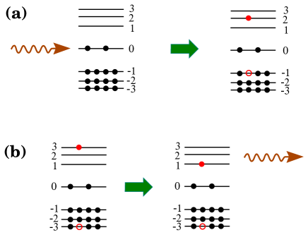
Figure 1: (color online) Different types of magneto-phonon resonance in excitation decay. (a) An optical phonon decaying into an electronic excitation. (b) An electronic excitation decaying into an optical phonon and another electronic excitation. The horizontal lines represent the Landau levels, the black circles represent their filling. The filled red circle represents the excited electron, the empty red circle represents the hole, and the wavy line represents the phonon.

In the following, we use a shorthand notation $L_{-n,m}$ for an excitation of an electron from a filled level $-n$ to an empty level $m$ (assuming that the partially filled level is $n=0$). To gain a qualitative insight into various resonant processes, it is instructive to analyze the weak coupling limit first. Namely, consider an initial excitation which was created in the sample in the course of Raman scattering, and analyze different channels of decay for this excitation (see Fig. 1).

One case is when the initial excitation is a phonon; for example, the doubly degenerate $E_{2g}$ phonon with the wave vector at the $\Gamma$ point of the first Brillouin zone, giving rise to the $G$ peak in the Raman spectrum. It may decay into an electronic inter-LL excitation, as schematically shown in Fig. 1(a). The selection rule for the matrix element is $n\to{n}\pm{1}$, so the phonon decay rate is strongly enhanced when the phonon is resonant with one of the corresponding transitions, that is, the phonon energy $\hbar\omega_{\Gamma}=E_{n+1}-E_{-n}=E_{n}-E_{-(n+1)}$ for some $n$. This case corresponds to the magneto-phonon resonance in the Raman scattering on phonons, which was observed experimentally Faugeras et al. (2009); Yan et al. (2010), following the theoretical prediction in Refs. Ando (2007); Goerbig et al. (2007).

In the present work, we focus on a different case, that of the initial excitation being an inter-LL excitation which decays into a phonon and another inter-LL excitation. Again, the corresponding decay rate is enhanced at resonance, but the resonance condition is different from the previous case. For example, if the initial excitation is $L_{-n,n}$, it can decay if the electron on the level $n$ or the hole on the level $-n$ emits a phonon and moves to another level $n^{\prime}$ or $-n^{\prime}$, respectively ($n^{\prime}<n$). The decay is resonant if the phonon energy $\hbar\omega=E_{n}-E_{n^{\prime}}$. It is essentially the same process that is responsible for the magneto-phonon resonance in electronic transport in semiconductors Gurevich and Firsov (1961); Puri and Geballe (1963); Shalyt et al. (1964), as well as in magneto-optical absorption Johnson and Larsen (1966); Korovin and Pavlov (1968).

The role of momentum conservation is quite different in the two processes. As we focus here on optical excitation, the momentum of the incident and scattered photons can be neglected, so in both cases, the total momentum of the initial excitation is zero. If the initial excitation is a single phonon, it can be only the $E_{2g}$ optical phonon from the $\Gamma$ point, and the total momentum of the inter-LL excitation into which it decays should also be zero, which leads to the selection rule $n\to{n}\pm{1}$, and thus restricts this case to the magneto-phonon resonance studied in Refs. Ando (2007); Goerbig et al. (2007); Faugeras et al. (2009); Yan et al. (2010). For a multi-phonon initial excitation, one can also think about the resonant enhancement of the phonon decay rate; however, the width of the multi-phonon Raman peaks is dominated by other factors than the phonon decay Basko (2008); Faugeras et al. (2010); Venezuela et al. (2011), so the modification of latter by the magnetic field is not observed in the Raman spectra.

For an initial electronic inter-LL excitation of zero total momentum, the momentum conservation allows the decay into a phonon with an arbitrary momentum and another inter-LL excitation with the opposite momentum. Still, the matrix element is strongly suppressed unless the phonon momentum is within $\sim{1}/l_{B}$ from the $\Gamma$ or $K,K^{\prime}$ points of the first Brillouin zone. Thus, one has to consider two kinds of resonances: (i) those involving the $E_{2g}$ optical phonons around the $\Gamma$ point and intravalley electronic inter-LL excitations, and (ii) those involving intervalley inter-LL excitations and phonons around the $K,K^{\prime}$ points. Among the latter phonons, those most strongly coupled to the electrons are the $A_{1g}$ transverse optical phonons. The corresponding phonon energies are $\hbar\omega_{\Gamma}=196\>\mbox{meV}$ and $\hbar\omega_{K}=160\>\mbox{meV}$ (see Sec. III). Another important consequence of finite phonon momenta ($\sim{1}/l_{B}$) involved in the process, is the absence of any selection rule on the LL indices. In the above example of the decay of the $L_{-n,n}$ excitation into a phonon and the $L_{-n,n^{\prime}}$, any $n^{\prime}$ is allowed (energy conservation requires $n^{\prime}<n$).

The above discussion of decay of the initial excitation is valid in the limit when the electron-phonon coupling is weak compared to the typical broadening of the Landau levels or to the dispersion of optical phonons or inter-LL excitations on the momentum scale $\sim{1}/l_{B}$. In the opposite limiting case, the problem corresponds to the coupling between discrete energy levels, when the states become strongly mixed. The energies of these hybrid excitations (magnetopolarons) exhibit an anticrossing as a function of the magnetic field as the latter is swept through the resonance region.

For an initial electronic inter-LL excitation, different types of resonances are possible. A resonance occurs when the phonon energy $\hbar\omega$ matches the energy difference between some empty Landau levels:

$$E_{n}-E_{n^{\prime}}=\hbar\omega,$$ (1)

for some $n>n^{\prime}\geqslant{0}$ (we assume to be at zero temperature and zero doping, so $n=0$ is the only partially filled level). Due to electron-hole symmetry, $E_{-n}=-E_{n}$, Eq. (1) automatically yields a similar condition for two filled levels, $E_{-n^{\prime}}-E_{-n}=\hbar\omega$. Also, because of the $\sqrt{n}$ dependence of $E_{n}$, the LLs are not equidistant, but still, some additional degeneracies may arise. For example, if $E_{4}-E_{1}=\hbar\omega$, this automatically yields $E_{1}-E_{0}=\hbar\omega$, while if $E_{3}-E_{2}=\hbar\omega$, there are no additional degeneracies.

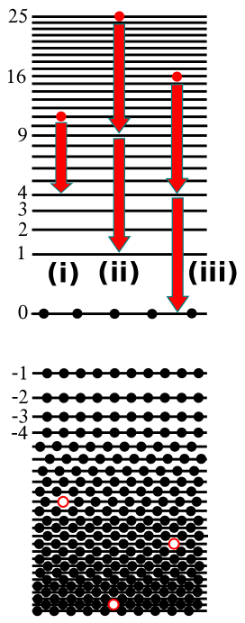
Figure 2: (color online) Examples of different consequences of a resonance of the type of Eq. (1). (i) Irrational $\zeta=\sqrt{11}/(\sqrt{11}-2)$ for the resonance $E_{11}=E_{4}+\hbar\omega$. No further resonant steps are possible. (ii) Rational $\zeta=5/2$ for the resonance $E_{25}=E_{9}+\hbar\omega$, which automatically yields the next resonant step, $E_{25}=E_{1}+2\hbar\omega$. The $n=0$ level is not involved. (iii) Integer $\zeta=2$ for the resonance $E_{16}=E_{4}+\hbar\omega$, which yields the next resonant step, $E_{16}=E_{0}+2\hbar\omega$, involving the partially filled zero level. The horizontal lines represent the Landau levels, the black circles represent their filling. The filled red circles represent the excited electrons, the vertical arrows show their transitions which are resonant with a phonon.

All resonances of the kind (1) can be classified into three groups, depending on whether the ratio

$$\zeta=\frac{E_{n}}{\hbar\omega}=\frac{\sqrt{n}}{\sqrt{n}-\sqrt{n^{\prime}}}$$ (2)

is integer, rational, or irrational (see Fig. 2). Let us see what happens in each of these cases, restricting our attention to the initial excitations of the type $L_{-n,n}$, which dominate the electronic Raman scattering in the magnetic field Kashuba and Fal’ko (2009), and to $L_{-(n+1),n}$ (as well as its electron-hole-symmetric counterpart $L_{-n,n+1}$), which are also observed in the Raman spectra, as discussed in Sec. III.

(i) If $\zeta$ is irrational, the resonances do not proliferate. Then the simplest case is that of the initial $L_{-(n+1),n}$ excitation which is resonant with $L_{-(n+1),n^{\prime}}$ plus one phonon. In this case, there are no hole resonances; indeed, $E_{-n^{\prime\prime}}-E_{-(n+1)}=\hbar\omega$ at the same time would imply $\sqrt{n+1}-\sqrt{n}=\sqrt{n^{\prime\prime}}-\sqrt{n^{\prime}}$ for some $n^{\prime}<n^{\prime\prime}<n$, which is impossible due to the concavity of the square root. The symmetric excitation $L_{-n,n}$ is then resonant with $L_{-n,n^{\prime}}$ (or $L_{-n^{\prime},n}$) plus one phonon, but also with $L_{-n^{\prime},n^{\prime}}$ plus two phonons, i. e. the electron and the hole resonances necessarily occur simultaneously. As the excitations with zero, one, and two phonons disperse differently with the magnetic field, the symmetric excitation gives a triple anticrossing of the levels as a function of the magnetic field. Such triple anticrossings were discussed long ago in the context of optical magnetoabsorption in bulk semiconductors Korovin (1971).

(ii) Let $\zeta$ be rational but not an integer, and let $m$ be the integer part of $\zeta$. In this case, condition (1) yields not just one, but $m$ resonances. Indeed, for any $j\leqslant{m}$ the energy $E_{n}-j\hbar\omega$ matches the energy $E_{n_{j}}$ of the level $n_{j}=[j\sqrt{n^{\prime}}-(j-1)\sqrt{n}]^{2}$. The last level in this sequence has the energy $E_{n_{m}}=(\zeta-m)\hbar\omega$, which does not allow for emission of any more phonons. However, if we construct $n_{m+1}=[(m+1)\sqrt{n^{\prime}}-m\sqrt{n}]^{2}$, then it turns out that $\sqrt{n_{m}}+\sqrt{n_{m+1}}=\sqrt{n}-\sqrt{n^{\prime}}$, or, equivalently, $\hbar\omega=E_{n_{m}}-E_{-n_{m+1}}$. This means that the phonon itself is resonantly hybridized with the electronic excitation from the filled level $-n_{m+1}$ to the empty level $n_{m}$ (as the phonon involved has a finite wave vector, there are no selection rules on $n_{m},n_{m+1}$). Thus, the asymmetric excitation $L_{-(n\pm{1}),n}$ is resonant with $L_{-(n\pm{1}),n_{j}}$ plus $j$ phonons for any $j=1,\ldots,m$, so we have an anticrossing of $m+1$ energy levels with different dispersions (the hybridization of the phonon with $L_{-n_{m+1},n_{m}}$ or $L_{-n_{m},n_{m+1}}$ does not add anything, as these electronic excitations disperse with the magnetic field in the same way as $E_{n}-E_{n^{\prime}}$). The symmetric excitation $L_{-n,n}$ can resonantly emit phonons both on the electron and hole sides, up to $2m$ phonons in total, corresponding to the anticrossing of $2m+1$ levels. It is important that for non-integer $\zeta$ none of the resonances involve the partially filled $n=0$ Landau level.

(iii) If $\zeta=m$, an integer, then the last term of the sequence $\{n_{j}\}$ from the previous case is $n_{m}=0$. The resonance counting is analogous to case (ii). Namely, we have $m+1$ anticrossings for the asymmetric initial excitation $L_{-(n\pm{1}),n}$ and $2m+1$ anticrossings for $L_{-n,n}$, so that the latter can thus be entirely transformed into $2m$ phonons by a sequence of resonant transitions. However, involvement of the partially filled $n=0$ level brings about a qualitatively new feature: the possibility of creation of an arbitrary number of zero-energy electronic excitations on the partially filled level. As will be discussed in Sec. IV.4, this feature makes a consistent theoretical treatment of case (iii) quite problematic.

Our experimental results, presented in Sec. III, include a clear observation of several resonances of type (iii) with double and, for the first time, triple avoided crossings. Near each avoided crossing, we describe our data phenomenologically by an effective two- or three-level model with some coupling between the resonant excitations. We also observe some signatures of resonances of type (i), which are, however, close to the limits of our experimental resolution, and they do not allow for a quantitative anlysis. Resonances of type (ii) are quite difficult to observe, as the smallest Landau level indices $n,n^{\prime}$ which produce non-integer rational $\zeta$ are $n=9$, $n^{\prime}=1$, leading to $\zeta=3/2$. The corresponding magnetic field is too low, and the Landau levels involved in the electronic excitation are too high, to be resolved in our experiment.

The theory for all three cases is presented in Sec. IV. Its main task is to justify (or disprove) the phenomenological description of each avoided crossing by an effective few-level model. Clearly, such description may be correct only if one can neglect the energy dispersion of the electronic excitations and of the phonons. The former can be neglected if the Coulomb interaction is sufficiently weak (e.g., due to screening by the conducting graphite substrate). As for the latter, one should recall that the most important contribution to the dispersion of phonons near the $\Gamma$ or $K$ points comes from their coupling to the Dirac electrons which produces the Kohn anomaly Piscanec et al. (2004); Grüneis et al. (2009). In a strong magnetic field the spectrum of Dirac electrons is quantized, so the main effect of the electron-phonon coupling is to induce magneto-phonon resonances. The residual part of the phonon dispersion which is due to interaction with electrons in the $\sigma$ bands is quite weak and can indeed be neglected, as the relevant scale of the phonon wave vectors is quite small, $q\sim{1}/l_{B}$ ($l_{B}$ is the magnetic length).

Still, it turns out, that even if one starts from dispersionless excitations, energy dispersion can be eventually generated due to resonant coupling. This effect is especially dramatic for case (iii), where plenty of zero-energy excitations are available on the partially filled $n=0$ Landau level. As a result, the splitting between the energies of the coupled excitations is accompanied by a broadening, whose magnitude is of the same order as the splitting. The broadened peaks have complicated spectral shapes, not described by any simple functional form, such as Lorentzian, Gaussian, or any other (see Fig. 11 in Sec. IV.4 for an example). Thus, the phenomenological description of our experimental data by effective two- or three-level models is very approximate.

The splitting of the $L_{0,1}$ electronic excitation, observed when it is in resonance with the $\Gamma$ point phonon near $B=28$ T Faugeras et al. (2009); Yan et al. (2010), can be ascribed to either of the two types of resonances mentioned in the beginning of this section. Indeed, on the one hand, it can be viewed as the decay of the initial phonon into an electronic excitation. On the other hand, it can also be viewed as the decay of the initial $L_{0,1}$ electronic excitation into a phonon and a zero-energy $L_{0,0}$ excitation, falling into case (iii) above. Due to such “double-faced” nature of this particular resonance, the split peaks are strongly broadened. This intrinsic broadening is missing in the simple description of Refs. Ando (2007); Goerbig et al. (2007). For the resonance between the $K$ point phonon and the $L_{0,1}$ excitation, coupling to an external continuum of states was introduced in Ref. Orlita et al. (2012) to describe the strong broadening of the peaks; here we see that the broadening, in fact, originates from the electron-phonon coupling itself, and there is no need to invoke any extrinsic effects.

The broadening effects are less dramatic in the cases (i) and (ii). As discussed above, case (ii) necessarily involves Landau levels with quite large $n\geqslant{9}$. This strongly suppresses the broadening effect: the main peaks are narrow and they contain the most of the spectral weight (Sec. IV.3). In case (i), discussed in Sec. IV.2, for asymmetric transitions $L_{-(n\pm{1}),n}$ no broadening is generated at all, so their resonance with $L_{-(n\pm{1}),n^{\prime}}$ and a phonon can be faithfully described by an effective two-level model. No broadening arises also for symmetric transitions $L_{-n,n}$ resonating with $L_{-n,n^{\prime}}$ and the $K$ point phonon, so the effective three-level description is justified. However, if $\Gamma$ point phonons are involved in the resonance, broadening is generated due to a peculiar phonon exchange effect: the phonons emitted by $L_{-n,0}$ and $L_{0,n}$ excitations which constitute the initial $L_{-n,n}$ excitation, can be reabsorbed in the opposite order; this is impossible for the $K$ point phonons as the two emitted phonons must necessarily belong to the opposite valleys.

III Experiment

The low-temperature magneto-Raman scattering response, at the µm scale, has been measured using a home-made miniaturized optical probe based on optical fibers (a 5 µm core mono-mode fiber for the excitation and a 50 µm core for the collection), lenses and optical band pass filters to clean the laser and to reject the laser line. The excitation laser at $\lambda=514.5$ nm is focused on the sample with a high numerical aperture aspherical lens down to a spot of the diameter $\sim 1$ µm. The sample is placed on piezo stages to allow for the spatial mapping of the Raman response of the sample. This optical set-up is inserted in a closed jacket, with some helium exchange gas, which is then immersed in liquid helium and placed in the center of resistive solenoid producing magnetic fields up to 30 T. The unpolarized Raman scattering response of our samples has been measured in the quasi-backscattering geometry with the magnetic field $B$ applied perpendicularly to the graphene crystal plane. This experimental set-up has been described in more details in Refs. Faugeras et al. (2011); Kossacki et al. (2012). To find a graphene flake on the surface of bulk graphite, we use the methodology based on the spatial mapping of the Raman scattering response of the surface of bulk graphite with an applied magnetic field described in Ref. Faugeras et al. (2014).

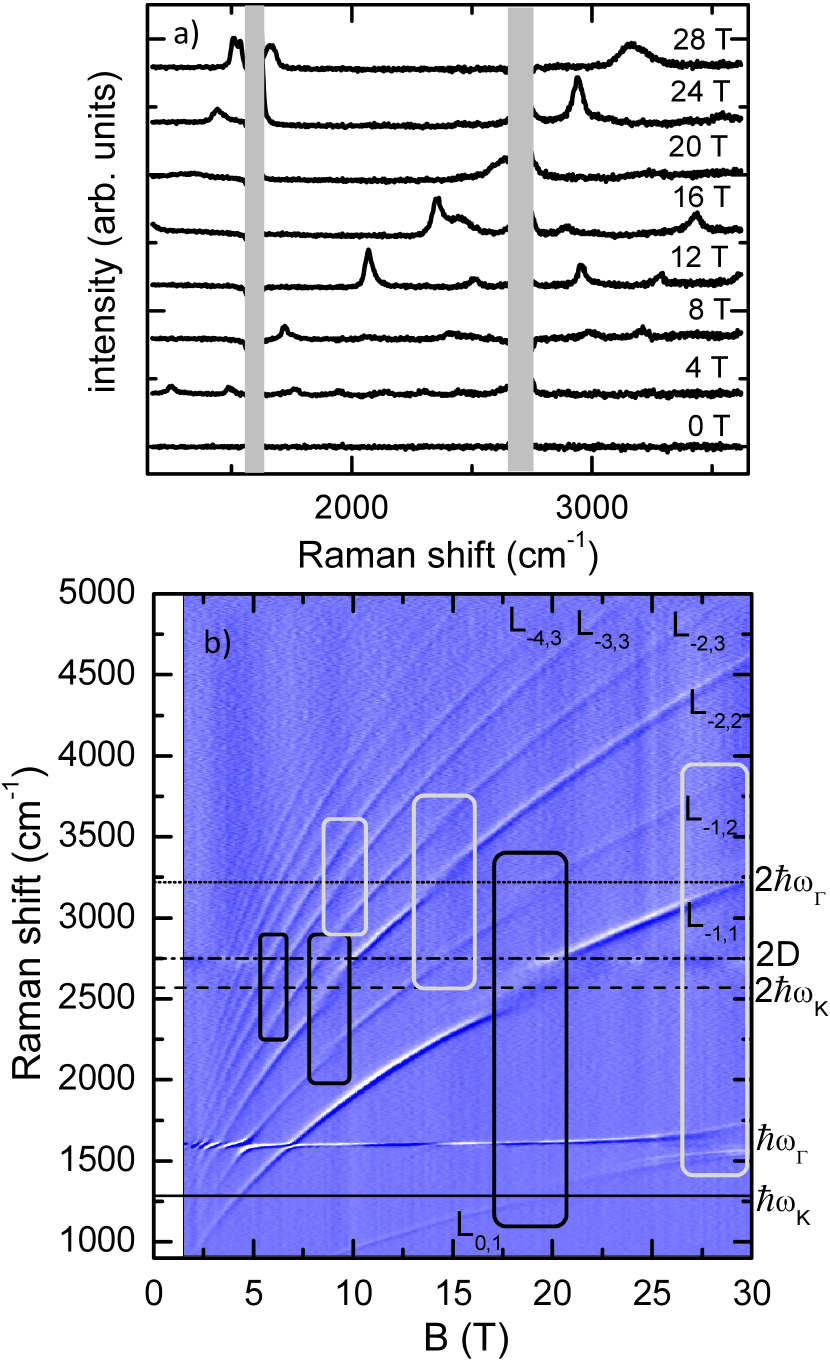
Figure 3: a) Characteristic Raman scattering spectra at selected values of the magnetic field, from which the zero-field response has been subtracted. The vertical gray bars mask the residual, after normalization, phonon contributions, due to the Faraday effect in the experimental set-up. b) False color map of the Raman scattering response of the graphene-like location, differentiated with respect to $B$, as a function of the magnetic field (with the step in $B$ of 100 mT). Main $L_{-n,m}$ electronic excitations are indicated. The horizontal solid line represents $\hbar\omega_{K}$, the dashed line $2\hbar\omega_{K}$, the dashed-dotted line is at the energy position of the 2D band feature while the dotted line represents $2\hbar\omega_{\Gamma}$. The three white (black) boxes identify spectral and magnetic field regions around $B=10,15$ and $28T$ ($B=6,9$ and $19T$) where the electron-$\Gamma$ point (K point) phonon resonance affects the spectra.

The typical Raman spectra, from which the $B=0$ response has been subtracted, are shown in Fig. 3(a). The two gray bars mask the two strong phonon features, the G band around $1582$ cm^-1 and the 2D band observed at $2750$ cm^-1 for our $514.5$ nm excitation. Typically, the observed line widths for electronic features are $\sim 30$ cm^-1. Due to the pronounced difference in the scattered intensity of phonon excitations and of the different types of electronic excitations, we present our main results in Fig. 3(b) in the form of a false color map of the scattered intensity as a function of the magnetic field which has been differentiated with respect to the magnetic field, with a step of $100$ mT. The 2D band feature is weakly affected by the magnetic field, but because of a Faraday effect affecting the intensity of the excitation laser when sweeping the magnetic field, it cannot be cleanly removed by normalizing spectra acquired at a finite field by the $B=0$ response. Thus, differentiation as a function of $B$ provides the cleanest color map.

The rich series of avoided crossings around $1582$ cm^-1 is due to the well-studied magneto-phonon resonance in the Raman scattering on the $\Gamma$-point optical phonon Ando (2007); Goerbig et al. (2007); Faugeras et al. (2009); Yan et al. (2010). In the following, instead of tracing the evolution of the phonon feature with $B$, we study the evolution of the inter-LL electronic excitations. This approach is today only possible for graphene on graphite which shows an exceptionally high quality Neugebauer et al. (2009), surpassing suspended graphene and graphene on BN Berciaud et al. (2014); Faugeras et al. (2015) in terms of line widths and of the variety of the observed excitations. The numerous features in Fig. 3(b) dispersing with the magnetic field can be attributed to inter-Landau-level electronic excitations Faugeras et al. (2011); Kühne et al. (2012), and in the present experiment they can be observed up to energies as high as $5000$ cm^-1. We observe $L_{-n,n}$ and $L_{-(n+1),n}$ (together with its electron-hole-symmetric counterpart $L_{-n,n+1}$) with $n$ up to 6. Their evolution with magnetic field can be reproduced using the value $v=(1.01\pm{0}.01)\times{1}0^{6}\>\mbox{m/s}$ for the electronic velocity in graphene.

magnetic field	resonant levels	transitions affected
28.5 T	$E_{1}=\hbar\omega_{\Gamma}$	$L_{0,1}$, $L_{-1,1}$, $L_{-1,2}$
18.7 T	$E_{1}=\hbar\omega_{K}$	$L_{0,1}$, $L_{-1,1}$, $L_{-1,2}$
14.2 T	$E_{2}=\hbar\omega_{\Gamma}$	$L_{-1,2}$, $L_{-2,2}$, $L_{-2,3}$
9.5 T	$E_{3}=\hbar\omega_{\Gamma}$	$L_{-2,3}$, $L_{-3,3}$, $L_{-3,4}$
9.4 T	$E_{2}=\hbar\omega_{K}$	$L_{-1,2}$, $L_{-2,2}$, $L_{-2,3}$
6.2 T	$E_{3}=\hbar\omega_{K}$	$L_{-2,3}$, $L_{-3,3}$, $L_{-3,4}$

Table 1: The values of the magnetic fields, evaluated theoretically, and the corresponding resonances which can be observed in Fig. 3(b).

The monotonous rise of the electronic excitation energies with the magnetic field in Fig. 3(b) is seen to be interrupted at several particular values of the magnetic field, identified by white and black boxes. These values of $B$ match very well those corresponding to the resonances $E_{n}=\hbar\omega_{K,\Gamma}$ for $n=1,2,3$, shown in Table 1. In the classification of Sec. II, all these resonances correspond to case (iii) with $\zeta=1$, so they are supposed to produce double anticrossings for $L_{-(n+1),n}$, $L_{-n,n+1}$ excitations, and triple anticrossings for $L_{-n,n}$ excitations. It is clearly seen in Fig. 3(b) that the resonance of $L_{-n,n}$ excitations with the two-phonon excitation occurs at an energy $2\hbar\omega_{K}\sim 2570$ cm^-1. This energy is different from that of the 2D band feature which involves phonons away from K point and which appears at higher energies (about 2700 cm^-1 for a $780$ nm excitation).

The difference between double anticrossings for antisymmetric excitations and triple anticrossings for symmetric excitations can be clearly seen in the Raman scattering spectra. In Fig. 4(a),(b) we show the spectra corresponding to the $L_{0,1}$ and to the $L_{-1,1}$ excitations, respectively, for selected values of the magnetic field close to $B=18$ T. In Fig. 4(a), the single peak observed at low magnetic field splits into two components with a gradual transfer of its intensity to the higher energy peak as $E_{1}$ crosses the phonon energy. This effect on the $L_{0,1}$ excitation has also been observed recently in infra-red magneto-transmission experiments performed on multi-layer epitaxial graphene Orlita et al. (2012). The evolution of the $L_{-1,1}$ excitation in this range of magnetic fields is completely different, as seen in Fig. 4(b): at the resonance, a three-peak structure appears. A similar triple avoided crossing can be observed also on the $L_{-2,2}$ when it is tuned to $2\hbar\omega_{K}$ at $B\sim 9$ T, and when L_-1,1 and L_-2,2 are tuned to $2\hbar\omega_{\Gamma}$, at $B\sim 28$ T and $B\sim 14$ T, respectively. Because the observed electronic excitations show a splitting, one can conclude that we are in the strong coupling regime and that magneto-polarons are formed at the resonant magnetic fields.

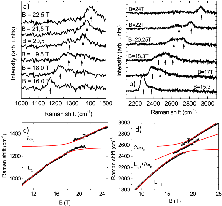
Figure 4: a) Spectra of $L_{0,1}$ electronic excitation in the range of magnetic field where it is in resonance with $K$ point phonons, showing an avoided crossing behavior. b) Spectra of the $L_{-1,1}$ electronic excitation in the same range of magnetic fields as in a), and showing a triple avoided crossing. c,d) $L_{0,1}$ and $L_{-1,1}$ energies, respectively, as a function of the magnetic field (black dots) together with calculated lines (solid lines).

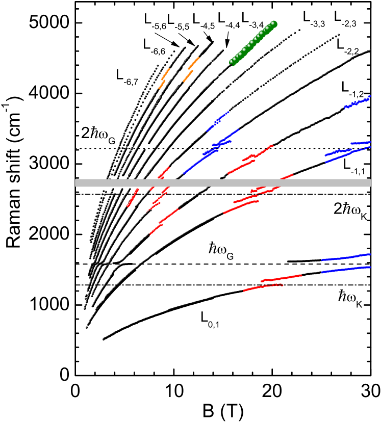
Figure 5: Magnetic field dependence of the main features observed in our Raman scattering spectra. Red points indicate resonances involving K-point phonons, blue point indicate resonances involving $\Gamma$-point phonons and orange points indicate the effects of the $E_{1,n(-n,-1)}=E_{K}$ resonance. Green circles represent the case (iii) resonance with $\zeta=2$ observed on the $L_{-3,4}$ excitation. The horizontal gray bar masks the residual contribution of the 2D band.

More avoided crossing features can be seen in Fig. 5, where we present the evolution of the maxima of the observed electronic excitation Raman scattering features as a function of the magnetic field. In this figure, in addition to the type (iii) resonances involving $K$-point and $\Gamma$-point phonons (red and blue points, respectively) mentioned in Table 1, some resonances of the type (i) resonances involving K-point phonons can be seen (shown by orange points). They correspond to the condition $E_{n}-E_{1}=\hbar\omega_{K}$, and are expected to occur at $B\approx 12.3,\,8.9,\,6.9$ and $5.6$ T for $n=5,6,7,8$, respectively. We present in Fig. 6(a) characteristic Raman scattering spectra between $B=9$ T and $B=14$ T and showing, among others, the $L_{-4,5}$ excitation. Close to $B=12$ T, the corresponding Raman feature splits into two components and then recovers its single-peak shape. Similar behavior is observed near $B=9$ T on the $L_{-5,6}$ excitation. Our experimental resolution is not sufficient for a quantitative analysis of this data. We have not been able to resolve avoided crossings at the same values of $B$ on $L_{-5,5}$ and $L_{-6,6}$ features. A possible reason for this is that for $L_{-n,n}$ the splitting is necessarily accompanied by the intrinsic broadening, as discussed in Sec. IV, which makes it harder to resolve than for asymmetric $L_{-(n-1),n}$ excitations. No type (i) resonances with $\Gamma$-point phonons are observed either; this may be due to weaker coupling of electrons to these phonons than to $K$ point phonons. Finally, the feature seen at $B=18.7$ T on $L_{-3,4}$ line corresponds to case (iii) with $\zeta=2$. The Raman scattering spectra of this excitation are presented in Fig. 6b) for $B=15.5,17.5$ and $18.5$ T. The single peak observed below $B=15$ T transforms into a broad feature at high magnetic fields. This evolution is also presented in Fig. 5 in the form of large green circles. Because of the lower sensitivity of our experimental setup at such high energies, we cannot fully resolve the line shape nor can we determine the number of components contributing to this feature at the resonance, although we expect that in this range of magnetic fields the resonance $E_{4}-E_{1}=E_{1}-E_{0}=\hbar\omega_{K}$ is relevant, so a triple avoided crossing should be observed.

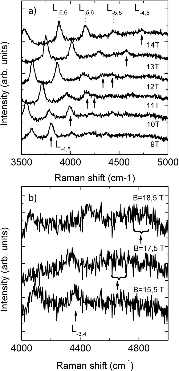
Figure 6: a) Raman scattering spectra ($B=0$ T subtracted) for selected values of the magnetic field showing the L_-5(-4),4(5) excitation splitting around $B=12$ T. At $B=14$ T, the principal electronic excitations are identified. b) Raman scattering spectra measured at $B=15.5,17.5$ and $18.5$ T in the range of energy of the $L_{-3,4}$ electronic excitation.

It is natural to describe a double or a triple avoided crossing phenomenologically by an effective two- or three-level problem with the Hamiltonian

$$H_{\mathrm{eff}}^{2\times{2}}=\left(\begin{array}[]{cc}E_{n}+E_{n\pm{1}}&C_{1}^{\prime}\hbar{v}/l_{B}\\ C_{1}^{\prime}\hbar{v}/l_{B}&E_{n\pm{1}}+\hbar\omega_{\mathrm{ph}}\end{array}\right),$$ (3c)

$$H_{\mathrm{eff}}^{3\times{3}}=\left(\begin{array}[]{ccc}2E_{n}&C_{1}\hbar{v}/l_{B}&0\\ C_{1}\hbar{v}/l_{B}&E_{n}+\hbar\omega_{\mathrm{ph}}&C_{2}\hbar{v}/l_{B}\\ 0&C_{2}\hbar{v}/l_{B}&2\hbar\omega_{\mathrm{ph}}\end{array}\right).$$ (3g)

Here $\omega_{\mathrm{ph}}$ is either $\omega_{K}$ or $\omega_{\Gamma}$, depending on which resonance is considered. The coupling between different levels is characterized by the natural energy scale $\hbar{v}/l_{B}$ and the dimensionless coefficients $C_{1}^{\prime},C_{1},C_{2}$. For the moment, we treat them as phenomenological fitting parameters, different for each avoided crossing. Their values, extracted from the fit to the experimental data are given in Table 2 for the crossings which are sufficiently well resolved to allow for a quantitative analysis.

The validity of the effective models (3c), (3g) is discussed in detail in Sec. IV.4, where we also give approximate relations between the phenomenological couplings $C_{1}^{\prime},C_{1},C_{2}$ and the dimensionless electron-phonon coupling constants $\lambda_{K},\lambda_{\Gamma}$. It is important that all resonances involving a given phonon (at either $K$ or $\Gamma$ point) are described by a single electron-phonon coupling constant, so the analysis of the whole set of avoided crossings, besides producing an estimate for $\lambda_{K},\lambda_{\Gamma}$, provides also a consistency check for the theory. The whole data is reasonably well described by $\lambda_{K}=0.05$, $\lambda_{\Gamma}=0.03$, and the comparison between theoretical and experimental values of the coefficients $C_{1}^{\prime},C_{1},C_{2}$ is given in Table 2.

transition	resonant levels	$C_{1}^{\prime}$ or $C_{1}$ (exp)	$C_{1}^{\prime}$ or $C_{1}$ (th)	$C_{2}$ (exp)	$C_{2}$ (th)
$L_{0,1}$	$E_{1}=\hbar\omega_{K}$	$0.044\pm 0.004$	0.045
$L_{-1,1}$	$E_{1}=\hbar\omega_{K}$	$0.056\pm 0.003$	0.063	$0.084\pm 0.005$	0.070
$L_{-1,2}$	$E_{1}=\hbar\omega_{K}$	$0.042\pm 0.003$	0.045
$L_{-1,2}$	$E_{2}=\hbar\omega_{K}$	$0.049\pm 0.004$	0.045
$L_{-2,2}$	$E_{2}=\hbar\omega_{K}$	$0.055\pm 0.004$	0.063	$0.088\pm 0.005$	0.072
$L_{-2,2}$	$E_{2}=\hbar\omega_{\Gamma}$	$0.044\pm 0.004$	0.049	$0.053\pm 0.005$	0.057
$L_{-2,3}$	$E_{2}=\hbar\omega_{\Gamma}$	$0.046\pm 0.003$	0.035

Table 2: The dimensionless couplings $C_{1}^{\prime},C_{1},C_{2}$ in the effective two- and three-level models (3c), (3g) for various avoided crossings observed in the experiment. The theoretical values are obtained from relations given in Sec. IV.4 with dimensionless electron-phonon coupling constants $\lambda_{K}=0.05$, $\lambda_{\Gamma}=0.03$.

IV Theory

IV.1 The model

In the Landau gauge, $A_{x}=-By$, the electronic states in graphene are labeled by four quantum numbers: (i) Landau level index $\ell$, which is an integer running from $-\infty$ to $+\infty$ (in the previous sections, we used $n=|\ell|$); (ii) the $x$ component of the momentum $p$, which can be taken to run from $0$ to $L_{y}/l_{B}^{2}$ with spacing $2\pi/L_{x}$ if one considers a finite rectangular sample of the size $L_{x}\times{L}_{y}$; (iii) the valley index, $K$ or $K^{\prime}$; (iv) the spin projection, which does not play any role in the following, so it will be omitted. The energy depends only on the Landau level index,

$$E_{\ell}=\frac{v}{l_{B}}\,\sqrt{2|\ell|}\,\mathop{\mathrm{sign}}\ell,$$ (4)

where the Dirac velocity $v\approx{1}.0\times{10}^{6}\>\mbox{m/s}\approx{6}.6\>\mbox{eV}\cdot\mbox{\AA}$, the magnetic length $l_{B}\approx(256\>\mbox{\AA})/\sqrt{B/(1\>\mbox{T})}$, and we set $\hbar=1$ throughout this section.

We consider electron coupling to two kinds of phonons: (i) the $A_{1g}$ transverse optical phonons near the $K$ or $K^{\prime}$ points, whose states are labeled by the valley index $K,K^{\prime}$, and the wave vector $\mathbf{q}$ counted from the corresponding point ($K$ or $K^{\prime}$); (ii) the $E_{2g}$ optical phonons near the $\Gamma$ point, labeled by the wave vector $\mathbf{q}$ and one of the two circular polarizations $\sigma=\pm$. We will neglect the phonon dispersion, so the frequencies of (i) and (ii) are $\omega_{\Gamma}\approx{196}\>\mbox{meV}$ and $\omega_{K}\approx{160}\>\mbox{meV}$. It should be emphasized that the most important contribution to the dispersion of phonons near the $\Gamma$ or $K$ points comes from their coupling to the Dirac electrons which produces the Kohn anomaly Piscanec et al. (2004); Grüneis et al. (2009). The coupling to the Dirac electrons is included in the Hamiltonian below, so the Kohn anomaly should not be included in the phonon dispersion to avoid double counting. Moreover, the spectrum of Dirac electrons is strongly modified by the magnetic field, so the resulting contribution to the phonon dispersion is quite different from the one at $B=0$. Thus, what is neglected here, is the mechanical part of the phonon dispersion which is due to the interaction with electrons in the $\sigma$ bands.

The Hamiltonian is taken in the form

$$\hat{H}=\hat{H}_{\mathrm{LL}}+\hat{H}_{\mathrm{ph},K}+\hat{H}_{\mathrm{ph},\Gamma}+\hat{H}_{\mathrm{int},K}+\hat{H}_{\mathrm{int},\Gamma}.$$ (5a)

The non-interacting part of the Hamiltonian is given by

$$\hat{H}_{\mathrm{LL}}=\sum_{\ell=-\infty}^{\infty}\sum_{p}E_{\ell}\left(\hat{c}^{\dagger}_{\ell,p,K}\hat{c}_{\ell,p,K}+\hat{c}^{\dagger}_{\ell,p,K^{\prime}}\hat{c}_{\ell,p,K^{\prime}}\right),$$ (5b)

$$\hat{H}_{\mathrm{ph},K}=\sum_{\mathbf{q}}\omega_{K}\left(\hat{b}^{\dagger}_{\mathbf{q},K}\hat{b}_{\mathbf{q},K}+\hat{b}^{\dagger}_{\mathbf{q},K^{\prime}}\hat{b}_{\mathbf{q},K^{\prime}}\right),$$ (5c)

$$\hat{H}_{\mathrm{ph},\Gamma}=\sum_{\mathbf{q}}\omega_{\Gamma}\left(\hat{b}^{\dagger}_{\mathbf{q},+}\hat{b}_{\mathbf{q},+}+\hat{b}^{\dagger}_{\mathbf{q},-}\hat{b}_{\mathbf{q},-}\right),$$ (5d)

where $$\hat{c}^{\dagger},\hat{c}$$ are the fermionic creation and annihilation for electrons in the corresponding single-particle states. The electron-phonon coupling is the same as in Ref. Basko (2008), but written in the Landau level basis:

$$\hat{H}_{K}=\sqrt{\frac{\lambda_{K}v^{2}}{L_{x}L_{y}}}\sum_{\mathbf{q}}\sum_{\ell,\ell^{\prime},p}\tilde{J}^{z}_{\ell,\ell^{\prime}}(-\mathbf{q})\,e^{ipq_{y}l_{B}^{2}}\left(\hat{b}^{\dagger}_{\mathbf{q},K}\hat{c}^{\dagger}_{\ell,p-q_{x}/2,K}\hat{c}_{\ell^{\prime}\!,\,p+q_{x}/2,K^{\prime}}+\hat{b}^{\dagger}_{\mathbf{q},K^{\prime}}\hat{c}^{\dagger}_{\ell,p-q_{x}/2,K^{\prime}}\hat{c}_{\ell^{\prime}\!,\,p+q_{x}/2,K}\right)+\mbox{h.c.},$$ (5e)

$$\hat{H}_{\Gamma}=\sqrt{\frac{\lambda_{\Gamma}{v}^{2}}{L_{x}L_{y}}}\sum_{\mathbf{q},\sigma}\sum_{\ell,\ell^{\prime},p}\tilde{J}^{-\sigma}_{\ell,\ell^{\prime}}(-\mathbf{q})\,e^{ipq_{y}l_{B}^{2}}\,\left(\hat{b}^{\dagger}_{\mathbf{q},\sigma}\hat{c}^{\dagger}_{\ell,p-q_{x}/2,K}\hat{c}_{\ell^{\prime}\!,\,p+q_{x}/2,K}-\hat{b}^{\dagger}_{\mathbf{q},\sigma}\hat{c}^{\dagger}_{\ell,p-q_{x}/2,K^{\prime}}\hat{c}_{\ell^{\prime}\!,\,p+q_{x}/2,K^{\prime}}\right)+\mbox{h.c.}.$$ (5f)

where “h.c.” stands for the Hermitian conjugate, and the dimensionless coupling constants $$\lambda_{K},\lambda_{\Gamma} \lambda_{\Gamma}\approx{0}.03 \lambda_{K} \lambda_{K}=0.05$$ are defined as in Ref. Basko (2008). While the value is established relatively well Pisana et al. (2007); Yan et al. (2007); Faugeras et al. (2009) and is also in agreement with our experimental results discussed in the previous section, the constant is subject to Coulomb enhancement Basko and Aleiner (2008); Lazzeri et al. (2008), and thus is substrate-dependent. For our samples of graphene on graphite, the Coulomb renormalization effects have been shown to be strongly suppressed by substrate screening Faugeras et al. (2015), so the enhancement should be relatively weak; our experimental data are reasonably well described by (see the previous section).

The coefficients $\tilde{J}^{z}_{\ell,\ell^{\prime}}(\mathbf{q})=[\tilde{J}^{z}_{\ell^{\prime},\ell}(-\mathbf{q})]^{*}$ and $\tilde{J}^{\pm}_{\ell,\ell^{\prime}}(\mathbf{q})=[\tilde{J}^{\mp}_{\ell^{\prime},\ell}(-\mathbf{q})]^{*}$, represent the matrix elements of the phonon-induced potential between the electronic eigenstates in the magnetic field, and are given by

$$\tilde{J}^{z}_{\ell,\ell^{\prime}}(\mathbf{q})={} {}\sqrt{(1+\delta_{\ell{0}})(1+\delta_{\ell^{\prime}{0}})}\,\frac{J_{|\ell|,|\ell^{\prime}|}(\mathbf{q})}{2}-{}$$

$${}-(1-\delta_{\ell{0}})(1-\delta_{\ell^{\prime}{0}})\mathop{\mathrm{sign}}(\ell\ell^{\prime})\frac{J_{|\ell|-1,|\ell^{\prime}|-1}(\mathbf{q})}{2},$$ (6a)

$$\tilde{J}^{+}_{\ell,\ell^{\prime}}(\mathbf{q})={} {}(1-\delta_{\ell{0}})\mathop{\mathrm{sign}}\ell\,\frac{\sqrt{1+\delta_{\ell^{\prime}0}}}{2}\,J_{|\ell|-1,|\ell^{\prime}|}(\mathbf{q}),$$ (6b)

$$\tilde{J}^{-}_{\ell,\ell^{\prime}}(\mathbf{q})={} {}(1-\delta_{\ell^{\prime}{0}})\mathop{\mathrm{sign}}\ell^{\prime}\,\frac{\sqrt{1+\delta_{\ell{0}}}}{2}\,J_{|\ell|,|\ell^{\prime}|-1}(\mathbf{q}).$$ (6c)

The formfactors,

$$J_{n,m}(\mathbf{q})={} {}(-1)^{m+\min\{n,m\}}\sqrt{\frac{\min\{n,m\}!}{\max\{n,m\}!}}\times{}$$

$${}\times e^{-q^{2}l_{B}^{2}/4}\,\left(\frac{q_{x}+iq_{y}}{q}\right)^{n-m}\left(\frac{ql_{B}}{\sqrt{2}}\right)^{|n-m|}\times{}$$

$${}\times\mathrm{L}_{\min\{n,m\}}^{(|n-m|)}(q^{2}l_{B}^{2}/2)=J_{m,n}^{*}(-\mathbf{q}),$$ (7)

are defined via the associated Laguerre polynomials,

$$\mathrm{L}_{m}^{(\alpha)}(\xi)=\sum_{k=0}^{m}\frac{(-1)^{k}(m+\alpha)!}{k!\,(m-k)!\,(\alpha+k)!}\,\xi^{k},$$ (8)

which satisfy the following orthogonality relation:

$$\int\limits_{0}^{\infty}\mathrm{L}_{n}^{(\alpha)}(\xi)\,\mathrm{L}_{m}^{(\alpha)}(\xi)\,x^{\alpha}e^{-x}\,dx=\frac{(n+\alpha)!}{n!}\,\delta_{nm}.$$ (9)

We are not interested in the Raman process itself, which was studied in detail in Ref. Kashuba and Fal’ko (2009). Our main focus is the spectral function of the electronic excitation, which was created in this process. The creation operators for the electronic excitations observed in the experiment, those of the type $-n\to{n}$, $-(n\pm{1})\to{n}$, can be represented as

$$\hat{R}_{n,j}^{\dagger}=\sum_{p}\hat{c}^{\dagger}_{n,p,K}\hat{c}_{-(n+j),p,K},\quad j=0,\pm{1},$$ (10)

where we have arbitrarily chosen the states in one valley, $K$, as the states in the other valley behave exactly in the same way. The spectral function can be obtained as $-(1/\pi)\mathop{\mathrm{Im}}\Pi_{n,j}(\Omega)$ from the excitation propagator

$$\Pi_{n,j}(\Omega)=-i\,\frac{2\pi{l}_{B}^{2}}{L_{x}L_{y}}\int\limits_{-\infty}^{\infty}\left\langle\mathrm{T}\,\hat{R}_{n,j}(t)\,\hat{R}_{n,j}^{\dagger}(0)\right\rangle e^{i\Omega{t}}\,dt,$$ (11)

where the average is over the ground state and T stands for the chronological time ordering.

The excitation propagator (11) is calculated using the standard zero-temperature diagrammatic technique Abrikosov et al. (1975), which is constructed from the following basic elements.

• The electron Green’s function, represented by a solid line, carries the energy variable $\epsilon$ and the indices of the single-particle states. It depends only on the energy and the Landau level index:

  $$G_{\ell}(\epsilon)=\frac{1}{\epsilon-E_{\ell}+i0^{+}\mathop{\mathrm{sign}}\ell}.$$ (12a)

  The sign of the infinitesimal imaginary part $$i0^{+} \ell<0 \ell>0 \ell=0 f_{0} p f_{0} G_{p}(\epsilon)=1/(\epsilon-i0^{+}) G_{p}(\epsilon)=1/(\epsilon+i0^{+})$$ corresponds to the Landau level filling: the levels with are filled, those with are empty. On the level only a fraction of states is assumed to filled. This can be modeled by introducing a fictitious dependence of the infinitesimal imaginary part on the momentum : we choose at random a fraction of the momenta for which we set , and for the rest it is . In the subsequent calculations it is equivalent to simply setting

  $$G_{\ell=0}(\epsilon)=\frac{1-f_{0}}{\epsilon+i0^{+}}+\frac{f_{0}}{\epsilon-i0^{+}}.$$ (12b)

• The phonon Green’s function, represented by a wavy line, carries the frequency variable $\omega$, the two-dimensional momentum $\mathbf{q}$, and one of the four labels $K,K^{\prime},+,-$ (the latter two correspond to the circular polarizations of the phonons near the $\Gamma$ point). The Green’s function is given by

  $$D_{K,\Gamma}(\omega)=\frac{1}{\omega-\omega_{K,\Gamma}+i0^{+}}.$$ (13)

  We do not include the negative-frequency part of the phonon Green’s function as the resonant approximation will be used in all subsequent calculations.

• The electron-phonon vertices are given by the coefficients in the interaction Hamiltonians $\hat{H}_{K,\Gamma}$ in Eqs. (5e), (5f).

In the absence of interactions, the excitation propagator is given by

$$\Pi_{n,j}^{(0)}(\Omega)={} {}\int\frac{d\epsilon}{2\pi{i}}\,G_{n}(\epsilon)\,G_{-(n+j)}(\epsilon-\Omega)={}$$

$$={} {}\frac{1}{\Omega-(E_{n}+E_{n+j})+i0^{+}},$$ (14)

so the spectral function is given by just a single $\delta$-peak $\delta(\Omega-(E_{n}+E_{n+j}))$.

IV.2 Irrational case

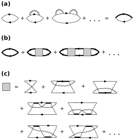
Figure 7: Diagrams contributing to the excitation propagator in the case (i) of Sec. II, (a) for the asymmetric transition $L_{-(n\pm{1}),n}$, (b) for the symmetric transition $L_{-n,n}$, with the vertex function given by (c). The thick solid line represents the dressed electronic Green’s function $\tilde{G}_{\pm{n}}(\epsilon)$, the shaded box represents the vertex function.

Let one of the phonon frequencies $\omega_{K,\Gamma}$ be close to the difference $E_{n}-E_{n^{\prime}}$ and $\zeta$ is irrational (equivalently, $\sqrt{n/n^{\prime}}$ is irrational). This is case (i) of Sec. II.

IV.2.1 Asymmetric transitions

For the asymmetric transition $-(n\pm{1})\to{n}$ the resonant contribution to $\Pi_{n,\pm{1}}(\Omega)$ is given by the sequence of diagrams shown in Fig. 7(a). It is sufficient to dress the electronic Green’s function $G_{n}(\epsilon)$ by the self-energy

$$\Sigma_{n}^{K}(\epsilon)=\lambda_{K}v^{2}\int\frac{d^{2}\mathbf{q}}{(2\pi)^{2}}\,\frac{|\tilde{J}^{z}_{nn^{\prime}}(\mathbf{q})|^{2}}{\epsilon-\omega_{K}-E_{n^{\prime}}+i0^{+}}=$$

$$\qquad=\frac{V_{K}^{2}}{\epsilon-\omega_{K}-E_{n^{\prime}}+i0^{+}},$$ (15a)

$$\Sigma_{n}^{\Gamma}(\epsilon)=\lambda_{\Gamma}{v}^{2}\int\frac{d^{2}\mathbf{q}}{(2\pi)^{2}}\,\frac{|\tilde{J}^{+}_{nn^{\prime}}(\mathbf{q})|^{2}+|\tilde{J}^{-}_{nn^{\prime}}(\mathbf{q})|^{2}}{\epsilon-\omega_{\Gamma}-E_{n^{\prime}}+i0^{+}}=$$

$$\qquad=\frac{V_{\Gamma}^{2}}{\epsilon-\omega_{\Gamma}-E_{n^{\prime}}+i0^{+}},$$ (15b)

$$V_{K,\Gamma}^{2}=\frac{\lambda_{K,\Gamma}v^{2}}{4\pi{l}_{B}^{2}},$$ (15c)

so that the dressed Green’s function is given by

$$\tilde{G}_{\pm{n}}(\epsilon)={} {}\frac{1}{G_{\pm{n}}^{-1}(\epsilon)-\Sigma_{\pm{n}}(\epsilon)}=$$

$$={} {}\frac{\epsilon\mp(\omega_{K,\Gamma}+E_{n^{\prime}})}{[\epsilon\mp(\tilde{E}_{n}^{+}-i0^{+})][\epsilon\mp(\tilde{E}_{n}^{-}-i0^{+})]},$$ (16)

where $\tilde{E}_{n}^{\pm}$ are the two roots of the equation

$$(\tilde{E}-E_{n})(\tilde{E}-E_{n}^{\prime}-\omega_{K,\Gamma})-V_{K,\Gamma}^{2}=0,$$ (17)

representing the energies of the two hybrid (magnetopolaron) states. The resulting excitation propagator,

$$\Pi_{n,\pm{1}}(\Omega)={} {}\int\frac{d\epsilon}{2\pi{i}}\,\tilde{G}_{n}(\epsilon)\,G_{-(n\pm{1})}(\epsilon-\Omega)=$$

$$={} {}\frac{\Omega-E_{n\pm{1}}-E_{n^{\prime}}-\omega_{K,\Gamma}}{(\Omega-E_{n\pm{1}}-\tilde{E}_{n}^{+})(\Omega-E_{n\pm{1}}-\tilde{E}_{n}^{-})},$$ (18)

where the positive infinitesimal imaginary part of $\Omega$ is omitted for compactness, coincides with the upper left element of the matrix $(\Omega-H_{\mathrm{eff}}^{2\times{2}})^{-1}$, where

$$H_{\mathrm{eff}}^{2\times{2}}=\left(\begin{array}[]{cc}E_{n\pm{1}}+E_{n}&V_{K,\Gamma}\\ V_{K,\Gamma}&E_{n\pm{1}}+E_{n^{\prime}}+\omega_{K,\Gamma}\end{array}\right)$$ (19)

can be viewed as the Hamiltonian of an effective two-level model. The resulting spectral function is given by the sum of two peaks $\delta(\Omega-\tilde{E}_{n}^{\pm})$ with the weights determined by the corresponding eigenvectors.

IV.2.2 Symmetric transitions

As discussed in Sec. II, in the case of a symmetric transition $-n\to{n}$, it is natural to expect the problem to be analogous to that of three coupled levels. However, the situation turns out to be qualitatively different for phonons near $K,K^{\prime}$ points and for those near $\Gamma$ point.

For the resonance $E_{n}-E_{n^{\prime}}\approx\omega_{K}$, it is sufficient to use the dressed Green’s function both for the electron on the level $n$ and for the hole on the level $-n$, Eq. (16), and to calculate $\Pi_{n,0}(\Omega)$ as in Eq. (14), but using the dressed Green’s functions instead of the bare ones. This corresponds to the first term in the sequence of diagrams shown in Fig. 7(b), and gives

$$\Pi_{n,0}(\Omega) {}=\int\frac{d\epsilon}{2\pi{i}}\,\tilde{G}_{n}(\epsilon)\,\tilde{G}_{-n}(\epsilon-\Omega)={}$$

$${}=\frac{(\Omega-E_{n}^{\prime}-\tilde{E}_{n}^{+})(\Omega-E_{n}^{\prime}-\tilde{E}_{n}^{-})-V_{K}^{2}}{(\Omega-2\tilde{E}_{n}^{+})(\Omega-2\tilde{E}_{n}^{-})(\Omega-\tilde{E}_{n}^{+}-\tilde{E}_{n}^{-})},$$ (20)

which is indeed equivalent [in the same sense as above, i. e. matching the upper left matrix element of $(\Omega-H_{\mathrm{eff}})^{-1}$] to an effective three-level system with the Hamiltonian

$$H_{\mathrm{eff}}^{3\times{3}}=\left(\begin{array}[]{ccc}2E_{n}&\sqrt{2}\,V_{K}&0\\ \sqrt{2}\,V_{K}&E_{n}+E_{n^{\prime}}+\omega_{K}&\sqrt{2}\,V_{K}\\ 0&\sqrt{2}\,V_{K}&2E_{n^{\prime}}+2\omega_{K}\end{array}\right).$$ (21)

Accordingly, the spectrum consists of three $\delta$ peaks.

For the resonance $E_{n}-E_{n^{\prime}}\approx\omega_{\Gamma}$, there are vertex corrections. This gives rise to the rest of the terms in Fig. 7(b), whose contribution is of the same order as the first one. The vertex, in turn, is represented by an infinite sum of diagrams, whose first terms are shown in Fig. 7(c). Physically, it corresponds to the electron and the hole exchanging the emitted phonons before their reabsorption. This process is possible only for the $\Gamma$ point phonons; for the $K,K^{\prime}$ phonons, those emitted by the electron and by the whole necessarily belong to different valleys, and cannot be exchanged, so all diagrams in Fig. 7(b) vanish except for the first one.

Inclusion of vertex corrections significantly increases the level of computational difficulty. Even though the diagrams for the vertex function can be summed, this summation reduces the problem to a system of integral equations for functions of momentum $\mathbf{q}$ with a non-separable kernel. These equations are given explicitly in Appendix A, where a different but equivalent formulation of the problem in terms of magnetopolaron wave functions is given. Solution of the resulting equations is beyond the scope of the present paper, but the qualitative properties of the result are worth discussing.

The dramatic effect of the phonon exchange is that the problem can no longer be effectively described in terms of a few coupled discrete levels. Let us note first that such description arose in the previous case only because we neglected the phonon dispersion as well as the dispersion of electronic excitations as a function of the total momentum. Had we included the dispersions, already in the simplest case of the self-energies (15a), (15b), they would not reduce to a simple single-pole form, so the spectral function $\mathop{\mathrm{Im}}\Pi_{n,\pm{1}}(\Omega)$, instead of being a sum of two $\delta$ peaks, would broaden into a continuum formed by excitations of different momenta. In the case of phonon exchange, even if one originally starts from non-dispersive excitations, the dispersion is produced as a result of the momentum-dependent coupling between the one-phonon and the two-phonon sectors, so the spectral function also broadens into a continuum with a non-trivial shape. It is important that this broadening should be of the same order as the splitting at resonance, as both are determined by the same energy scale $V_{\Gamma}$.

IV.2.3 Phonon dispersion

The phonon frequencies acquire a resonant correction when $\omega_{K}$ or $\omega_{\Gamma}$ is close to the energy $E_{n}-E_{-n^{\prime}}$ of a transition between filled and empty states. For $\sqrt{n/n^{\prime}}$ irrational, such resonances are distinct from those analysed above. The shifted frequencies can be found from the equation $\tilde{D}_{K,\Gamma}^{-1}(\mathbf{q},\omega)=0$, where the dressed phonon Green’s functions $\tilde{D}_{K,\Gamma}(\mathbf{q},\omega)$ are given by the diagrams shown in Fig. 8(a). Summation of the series gives

$$\tilde{D}_{K}^{-1}(\mathbf{q},\omega)=\omega-\omega_{K}-4V_{K}^{2}\,\frac{|\tilde{J}^{z}_{n,-n^{\prime}}(\mathbf{q})|^{2}+|\tilde{J}^{z}_{n^{\prime},-n}(\mathbf{q})|^{2}}{\omega-E_{n}-E_{n^{\prime}}+i0^{+}},$$ (22a)

$$\tilde{D}_{\Gamma}^{-1}(\mathbf{q},\omega)=\omega-\omega_{\Gamma}-8V_{\Gamma}^{2}\,\frac{|\tilde{J}^{\sigma}_{n,-n^{\prime}}(\mathbf{q})|^{2}+|\tilde{J}^{\sigma}_{n^{\prime},-n}(\mathbf{q})|^{2}}{\omega-E_{n}-E_{n^{\prime}}+i0^{+}}.$$ (22b)

The coefficient is twice larger for the $\Gamma$ phonons (8 instead of 4) because they can excite intravalley electron-hole pairs in any valley, while a $K$ phonon can excite an electron in $K^{\prime}$ valley and a hole in $K$ valley only (the spin degeneracy has also been taken into account).

The roots of the quadratic equation $\tilde{D}_{K,\Gamma}^{-1}(\mathbf{q},\omega)=0$ for each $\mathbf{q}$ give two frequencies of the coupled excitations which are superpositions of the phonon and the electronic excitations. As $J_{nn^{\prime}}(\mathbf{q})$ quickly falls off for $q\gg{1}/l_{B}$, the resonance modifies the phonon dispersion in the region $q\sim{1}/l_{B}$, $|E_{n}+E_{n}^{\prime}-\omega_{K,\Gamma}|\sim{V}_{K,\Gamma}$, and the typical magnitude of the frequency shift in this region is given by $V_{K,\Gamma}\sim\sqrt{\lambda_{K,\Gamma}}\,v/l_{B}$. This square-root dependence on the coupling constant should be contrasted to the Kohn-anomaly correction to the phonon dispersion without magnetic field, which is of the order of $\lambda_{K,\Gamma}vq$.

IV.3 Rational case

The smallest Landau level indices $n,n^{\prime}$ which produce a non-integer rational $\zeta$ are $n=9$, $n^{\prime}=1$, leading to $\zeta=3/2$. Even this resonance, $E_{9}-E_{1}=\omega_{K,\Gamma}$, is beyond our experimental resolution. Still, it is not too far from the observed resonance $E_{6}-E_{1}=\omega_{K,\Gamma}$, so the perspective of observing the $E_{9}-E_{1}=\omega_{K,\Gamma}$ resonance in the future is not totally hopeless. For more complicated cases, such as $E_{16}-E_{1}=\omega_{K,\Gamma}$ giving $\zeta=4/3$, or $E_{25}-E_{9}=\omega_{K,\Gamma}$ giving $\zeta=5/2$, there is not even such hope. Thus, here we focus on the simplest case $E_{9}-E_{1}=\omega_{K,\Gamma}$.

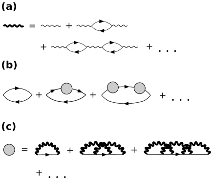
Figure 8: Diagrams contributing to the excitation propagator $\Pi_{9,\pm{1}}(\Omega)$. (a) Dressed phonon Green’s function. (b) Excitation propagator for the asymmetric transitions $L_{-8,9}$, $L_{-10,9}$ with the electronic self-energy given by (c). The thick wavy line represents the dressed phonon Green’s function $\tilde{D}_{K,\Gamma}(\mathbf{q},\omega)$, the shaded circle represents the electronic self-energy.

The difference of this resonance from those discussed in Sec. IV.2 is that the condition $E_{9}-E_{1}=\omega_{K,\Gamma}$ automatically yields $\omega_{K,\Gamma}=E_{1}-E_{-1}$. Thus, the emitted phonon can be resonantly reabsorbed by an electron on the level $n=-1$, creating a second electron-hole pair, in addition to the one initially produced by the photon (the energy of the resulting excitation is the same as that of the original excitation, as $E_{9}+E_{-1}=2E_{1}$). Thus, we dress the phonon Green’s function, as shown in Fig. 8(a):

$$\tilde{D}_{K}(\mathbf{q},\omega)=\left[\omega-\omega_{K}-\frac{4V_{K}^{2}|\tilde{J}^{z}_{1,-1}(\mathbf{q})|^{2}}{\omega-2E_{1}+i0^{+}}\right]^{-1},$$ (23a)

$$\tilde{D}_{\Gamma}(\mathbf{q},\omega)=\left[\omega-\omega_{\Gamma}-\frac{8V_{\Gamma}^{2}|\tilde{J}^{\sigma}_{1,-1}(\mathbf{q})|^{2}}{\omega-2E_{1}+i0^{+}}\right]^{-1}.$$ (23b)

For the asymmetric transitions, $L_{-8,9}$ and $L_{-10,9}$, the excitation propagator $\Pi_{9,\pm{1}}(\Omega)$ is given by the series in Fig. 8(b), where the electronic Green’s function is dressed by the self-energy insertions. As in Sec. IV.2.2, there is a difference between the coupling to $K,K^{\prime}$ phonons and to $\Gamma$ phonons, related to exchange. Namely, when the initial excitation (say, $L_{-8,9}$) is resonantly converted into $L_{-8,1}$ and one $K$ or $K^{\prime}$ phonon, and then into $L_{-8,1}+L_{-1,1}$, the two electrons on the $n=1$ level must belong to different valleys, and thus are effectively distinguishable. As a result, in the series for the self-energy, shown in Fig. 8(c), only the first term survives for $K,K^{\prime}$ phonons, resulting in a relatively compact expression:

$$\Sigma_{9}^{K}(\epsilon)={} {}\lambda_{K}v^{2}\int\frac{d^{2}\mathbf{q}}{(2\pi)^{2}}\,|\tilde{J}^{z}_{91}(\mathbf{q})|^{2}\tilde{D}_{K}(\mathbf{q},\epsilon-E_{1})=$$

$$={} {}\int\limits_{0}^{\infty}\frac{V_{K}^{2}(\epsilon-E_{9})(\xi-6)^{2}\xi^{8}e^{-\xi}\,d\xi/(2\cdot{9}!)}{(\epsilon-E_{9})(\epsilon-\omega_{K}-E_{1})-V_{K}^{2}(\xi-2)^{2}e^{-\xi}}.$$ (24)

Then the excitation propagator is straightforwardly evaluated as

$$\Pi_{9,\pm{1}}(\Omega)=\frac{1}{\Omega-(E_{9}+E_{9\pm{1}})-\Sigma_{9}^{K}(\Omega-E_{9\pm{1}})}.$$ (25)

As discussed in Sec. IV.2.2, as soon as excitations involved in the decay of the initial electron-hole pair acquire a dispersion, the peaks in the spectral function broaden and the situation can no longer be reduced to a simple effective picture of a few coupled discrete levels. This is what happens here, due to the phonon dispersion acquired from the resonant coupling to $L_{-1,1}$ electronic excitation, as seen from Eqs. (23a), (23b). However, in the present case, this effect turns out to be strongly suppressed due to the large Landau level index $n=9$. Let us formally expand the self-energy $\Sigma_{9}^{K}(\epsilon)$ from Eq. (24) at $V_{K}^{2}/[(\epsilon-E_{9})(\epsilon-\omega_{K}-E_{1})]\to\infty$:

$$\Sigma_{9}^{K}(\epsilon)={} {}\frac{V_{K}^{2}}{\epsilon-\omega_{K}-E_{1}}\times$$

$${}\times\left[1+\frac{5}{2048}\,\frac{V_{K}^{2}}{(\epsilon-E_{9})(\epsilon-\omega_{K}-E_{1})}+\ldots\right].$$ (26)

At resonance, $V_{K}^{2}\sim(\epsilon-E_{9})(\epsilon-\omega_{K}-E_{1})$, the second term in the square brackets is still small because of the numerical factor. The origin of this numerical smallness is that the numerator of the integrand in Eq. (24) has a maximum at $\xi\approx{12}$ and is very small at $\xi<7$, while the function $(\xi-2)^{2}e^{-\xi}$ in the denominator is quite small for $\xi>2$. Physically, this means that the electronic transition from level $n=9$ to $n=1$ is accompanied by emission of phonons with wave vectors $q=\sqrt{2\xi}/l_{B}$ which are too large and do not efficiently couple to $L_{-1,1}$ excitation.

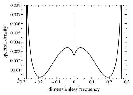
Figure 9: The dimensionless spectral density, $-(V_{K}/\pi)\mathop{\mathrm{Im}}\Pi_{9,\pm{1}}(\Omega)$, versus the dimensionless frequency $z=(\Omega-E_{9}/2+E_{-9\pm{1}})/V_{K}$ for the case of exact resonance, $E_{9}-E_{1}=\omega_{K}$. The square-root-type singularities at $z=\pm{2}e^{-2}\approx\pm{0}.27$ correspond to the maximum of $(\xi-2)e^{-\xi/2}$, the dimensionless energy splitting between the phonon and the $L_{-1,1}$ excitation [see Eq. (24)]. The spectral density for $|z|>2e^{-2}$ is extremely small, $\sim{10}^{-6}$, but finite; it vanishes exactly for $|z|>2$. The two main peaks are located near $z=\pm{1}$ (not shown). The singularity at $z\to{0}$ is logarithmic and comes from large $\xi$.

In the first approximation, if we neglect all terms in Eq. (26) except the first one, which is equivalent to replacing the dressed Green’s function $\tilde{D}_{K}(\mathbf{q},\omega)$ by the bare one, i. e., neglecting the coupling of the phonon to $L_{-1,1}$ excitation, we naturally obtain the effective $2\times{2}$ problem,

$$H_{\mathrm{eff}}^{2\times{2}}=\left(\begin{array}[]{cc}E_{9}&V_{K}\\ V_{K}&E_{1}+\omega_{K}\end{array}\right),$$ (27)

whose two eigenvalues $\tilde{E}_{9}^{\pm}$ determine the positions of two $\delta$ peaks in the spectral function. When the full self-energy (24) is taken into account, the two peaks (i) shift (the shift being equal in magnitude and opposite in sign for the two peaks), (ii) broaden [as $\mathop{\mathrm{Im}}\Sigma_{9}^{K}(\tilde{E}^{\pm}_{9})\neq{0}$, although very small], and (iii) lose a small part of their spectral weight. This part of the spectral weight is transferred to the continuum concentrated in the vicinity of the energies of the uncoupled excitations; in this region the spectral function has a peculiar shape, as illustrated in Fig. 9 for the case of exact resonance, $E_{9}-E_{1}=\omega_{K}$. At the same time, the two main peaks have nearly Lorentzian shapes, determined by the poles of $\Pi_{9,j}(\Omega)$ in the complex plane. The poles are located at

$$\Omega={} {}E_{9+j}+\frac{E_{9}+E_{1}+\omega_{K}}{2}\pm$$

$${}\pm\sqrt{\frac{(E_{9}-E_{1}-\omega_{K})^{2}}{4}+V_{K}^{2}u_{\pm}},$$ (28)

where $u_{\pm}\approx 1.00251\pm 0.66\times{10}^{-6}\,i$ are the solutions of the equation

$$0=\mathcal{F}(u)\equiv 1-\int\limits_{0}^{\infty}\frac{(\xi-6)^{2}\xi^{8}e^{-\xi}}{u-(\xi-2)^{2}e^{-\xi}}\,\frac{d\xi}{2\cdot{9}!},$$ (29)

and the sum of the residues at the two poles is given by

$$\left[u\,\frac{d\mathcal{F}(u)}{du}\right]^{-1}\approx 0.9975.$$

Thus, corrections to the simple two-level picture of Eq. (27) are quite small and will be masked by other effects, not included in the present model.

The same can be said about the case of coupling to $\Gamma$ point phonons. Even though the self-energy, corresponding to the sum of diagrams in Fig. 8,

$$\Sigma_{9}^{\Gamma}(\epsilon)={} {}\sum_{k=1}^{\infty}\sum_{\sigma_{1}\ldots\sigma_{k}}\int\frac{d^{2}\mathbf{q}_{1}\ldots d^{2}\mathbf{q}_{k}}{(\pi/l_{B}^{2})^{k}}\,\tilde{J}^{\sigma_{1}}_{91}(\mathbf{q}_{1})\,[\tilde{J}^{\sigma_{k}}_{91}(\mathbf{q}_{k})]^{*}\times{}$$

$${}\times\prod_{j=1}^{k-1}[\tilde{J}^{\sigma_{j}}_{1,-1}(\mathbf{q}_{j})]^{*}\tilde{J}^{\sigma_{j+1}}_{1,-1}(\mathbf{q}_{j+1})\,e^{i[\mathbf{q}_{j}\times\mathbf{q}_{j+1}]_{z}l_{B}^{2}}\times{}$$

$${}\times V_{\Gamma}^{2k}\,\frac{\tilde{D}_{K}(\mathbf{q}_{1},\epsilon-E_{1})\ldots\tilde{D}_{K}(\mathbf{q}_{k},\epsilon-E_{1})}{(E_{9}-\epsilon-i0^{+})^{k-1}},$$ (30)

is not easily evaluated, the factor $\tilde{J}^{\sigma}_{91}(\mathbf{q})$ will again result in an efficient coupling to phonons with relatively large wave wave vectors, which disperse very little. The same argument applies to the case of the symmetric transition $L_{-9,9}$. Thus, for all practical purposes, the case of rational $\zeta$ can be considered equivalent to the irrational case.

IV.4 Integer case

Among integer values of $\zeta$, the most interesting one is $\zeta=1$, that is, the resonance between the excitation $E_{n}-E_{0}$ and a phonon. This corresponds to the most pronounced features in the experimental data presented in Sec. III. The next value, $\zeta=2$, corresponds to the resonance $E_{n}-E_{n/4}=\omega_{K,\Gamma}$. A signature of this resonance is seen as broadening of the $L_{-3,4}$ transition around $B\approx{18}\>\mbox{T}$, but the resolution is not sufficient for a reliable quantitative analysis of the data. At the same time, the experimental data for $\zeta=1$ resonances do allow for a quantitative analysis.

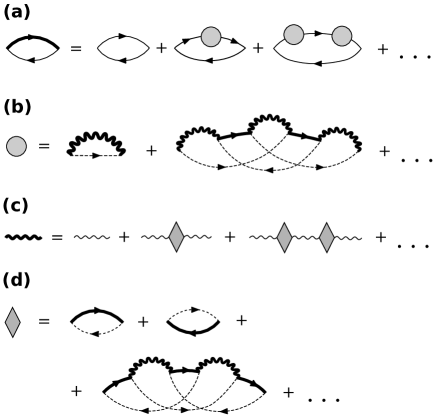
Figure 10: (a) Diagrams contributing to the excitation propagator $\Pi_{n,\pm{1}}(\Omega)$ for $n>1$. (b) The first terms of the series for the electronic self-energy which defines the dressed Green’s functions $\tilde{G}_{\pm{n}}(\epsilon)$. (c) Dressed phonon Green’s function, defined via the phonon polarization operator, the first diagrams for which are shown in (d). Thick solid lines represent the dressed electron Green’s functions on the $n$th Landau level. Dashed lines represent the bare electron Green’s functions on the partially filled zero Landau level. Thick wavy lines represent the dressed phonon Green’s function. Shaded circles represent the electronic self-energy. Shaded rhombi represent the phonon polarization operator.

From the theoretical point of view, description of resonances with integer $\zeta$ represents an extremely hard problem. In Fig. 10 we show diagrams contributing to the excitation propagator $\Pi_{n,\pm{1}}(\Omega)$ in the simplest case of the asymmetric transition $L_{-(n\pm{1}),n}$ when $E_{n}-E_{0}$ is resonant with a phonon ($\zeta=1$) and $n>1$ [for $L_{0,1}$ transition, the diagrams for $\Pi_{1,-1}$ are the same as in Fig. 10(c)]. The role of electrons on the partially filled $n=0$ level is emphasized by representing their Green’s function by a dashed line. In fact, we are unable to identify a dominant sequence of diagrams. The physical reason for this is the macroscopic degeneracy of the electronic non-interacting ground state due to partial filling of the $n=0$ Landau level. As a result, conversion of the initial electronic excitation with energy $E_{n}$ into the phonon and back can be accompanied by emission of an arbitrary number of intra-Landau-level excitations which cost no energy and can be exchanged in arbitrary order. Thus, various diagrams can be generated. In the resonant region, $|E_{n}-\omega_{K,\Gamma}|\sim{V}_{K,\Gamma}$, all these diagrams are of the same order, and there is no parameter for selection of a treatable subset of diagrams. As a result, the coupled levels broaden into a continuum, and we are not even able to write a closed set of integral equations to describe this broadening.

A qualitative description of this broadening effect can be done by keeping only the first diagram in Fig. (10)(b) and the first two diagrams in Fig. (10)(d). This procedure, analogous to the $GW$ approximation for interacting electrons (see Ref. Aryasetiawan and Gunnarsson (1998) for a review), gives a closed system of self-consistent equations for the dressed electron and phonon Green’s functions, $\tilde{G}$ and $\tilde{D}$. For the coupling to the $K$ point phonons this system has the following form:

$$\tilde{D}_{K}^{-1}(\mathbf{q},\omega)=\omega-\omega_{K}-4V_{K}^{2}\left[f_{0}|\tilde{J}_{n0}^{z}(\mathbf{q})|^{2}\tilde{G}_{n}(\omega)\right.-$$

$$\hskip 56.9055pt-\left.(1-f_{0})|\tilde{J}_{0,-n}^{z}(\mathbf{q})|^{2}\tilde{G}_{-n}(-\omega)\right],$$ (31a)

$$\tilde{G}_{n}^{-1}(\epsilon)=\epsilon-E_{n}-(1-f_{0})\lambda_{K}{v}^{2}\times$$

$$\hskip 56.9055pt{}\times\int\frac{d^{2}\mathbf{q}}{(2\pi)^{2}}\sum_{\sigma}|\tilde{J}_{n0}^{z}(\mathbf{q})|^{2}\tilde{D}_{K}(\mathbf{q},\epsilon),$$ (31b)

$$\tilde{G}_{-n}^{-1}(-\epsilon)=-\epsilon+E_{n}+f_{0}\lambda_{K}{v}^{2}\times$$

$$\hskip 51.21504pt{}\times\int\frac{d^{2}\mathbf{q}}{(2\pi)^{2}}\sum_{\sigma}|\tilde{J}_{0,-n}^{z}(\mathbf{q})|^{2}\tilde{D}_{K}(\mathbf{q},\epsilon),$$ (31c)

where $0<f_{0}<1$ is the filling of the zero Landau level. For the resonance with $\Gamma$ point phonons, the phonons corresponding to the two circular polarizations are dressed differently (unless $f_{0}=1/2$), so the above equations should be modified by (i) replacing $\tilde{D}_{K}\to\tilde{D}_{\sigma}$, $\tilde{J}^{z}\to\tilde{J}^{\sigma}$, and (ii) introducing an additional factor of two in the first equation, $4V_{K}^{2}\to{8}V_{K}^{2}$, due to the valley degeneracy. Restricting ourselves to the electron-hole-symmetric case with $f_{0}=1/2$, we eliminate the phonon Green’s function, and obtain a single algebraic equation for $\tilde{G}_{n}(\epsilon)=-\tilde{G}_{-n}(-\epsilon)$:

$$\frac{1}{\tilde{G}_{n}(\epsilon)}=\epsilon-E_{n}-\int\frac{\pi{l}_{B}^{2}V_{K}^{2}|J_{n0}(\mathbf{q})|^{2}\,{d^{2}\mathbf{q}}/{(2\pi)^{2}}}{\epsilon-\omega_{K}-2V_{K}^{2}|J_{n0}(\mathbf{q})|^{2}\tilde{G}_{n}(\epsilon)}.$$ (32)

The equation for the resonance with the $\Gamma$ phonon is obtained from this one by replacements $\omega_{K}\to\omega_{\Gamma}$, $V^{2}_{K}\to{V}^{2}_{\Gamma}$, $|J_{n0}(\mathbf{q})|^{2}\to|J_{n-1,0}(\mathbf{q})|^{2}$. It is convenient to introduce dimensionless variables $z=(\epsilon-\omega_{K})/V_{K}$ and $g(z)=V_{K}\tilde{G}_{n}(\epsilon)$, as well as the dimensionless detuning $\delta=(E_{n}-\omega_{K})/V_{K}$. Then the Raman spectrum for the asymmetric excitation, $(-1/\pi)\mathop{\mathrm{Im}}\Pi_{n,\pm{1}}(\Omega)=(-1/\pi)\mathop{\mathrm{Im}}\tilde{G}_{n}(\Omega-E_{n\pm{1}})\propto(-1/\pi)\mathop{\mathrm{Im}}{g}(z)$. The latter quantity, obtained from the numerical solution of Eq. (32) (see Appendix B for discussion of some properties of this equation) is plotted in Fig. (11) for $n=2$ and two values of detuning $\delta=0,1$.

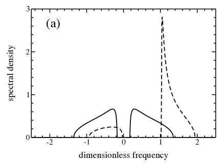
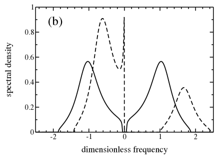
Figure 11: The dimensionless spectral densities (a) of the asymmetric electronic excitation, $-(V_{K}/\pi)\mathop{\mathrm{Im}}\Pi_{2,\pm{1}}(\Omega)$, and (b) of the $\Gamma$ point phonon, $(-V_{\Gamma}/\pi)\mathop{\mathrm{Im}}\tilde{D}_{\Gamma}(\mathbf{q}=0,\omega)$, versus the dimensionless frequency (a) $z=(\Omega-\omega_{K}+E_{-9\pm{1}})/V_{K}$, and (b) $z=(\omega-\omega_{\Gamma})/V_{\Gamma}$, as obtained from the $GW$ approximation. On both panels, the solid line correponds to the case of exact resonance, $\delta=(E_{2,1}-\omega_{K,\Gamma})/V_{K,\Gamma}=0$, the dashed line to $\delta=1$. The spikes for $\delta=1$ do not correspond to any divergencies in the spectral function, they are sharp but finite.

The same discussion can be applied to the magnetophonon resonance in the Raman scattering on the $\Gamma$-point phonons, seen as the resonant modulation of the $G$ peak Faugeras et al. (2009); Yan et al. (2010). The theory developed in Refs. Ando (2007); Goerbig et al. (2007), when considered close to each resonance, essentially maps on an effective two-level problem. This is correct for transitions not involving the zero Landau level, whose partial filling makes the picture for the $L_{0,1}$ transition more complicated, on the same level of difficulty as discussed above. Indeed, the Raman spectrum in this case is proportional to the phonon spectral function, $(-1/\pi)\mathop{\mathrm{Im}}\tilde{D}_{K}(\mathbf{q}=0,\omega)$, given by the diagrams of Fig. 10(b). The effect is illustrated in the same $GW$ approximation in Fig. 11(b), where we plot the spectrum $(-1/\pi)\mathop{\mathrm{Im}}[1/(z-g(z))]\propto(-1/\pi)\mathop{\mathrm{Im}}\tilde{D}_{\Gamma}(\mathbf{q}=0,\omega)$, obtained from the numerical solution of Eq. (32), modified to describe the coupling to the $\Gamma$ phonons, using $V_{\Gamma}$ as the unit of energy and introducing the shifted frequency $z=(\omega-\omega_{\Gamma})/V_{\Gamma}$, and for two values of detuning $\delta=(E_{1}-\omega_{\Gamma})/V_{\Gamma}=0$ and 1.

The $GW$ calculation, presented above, is not justified by any small parameter; near the resonance, the diagrams in Fig. 10(c,d) which are neglected, are of the same order as those that are retained. So there is no reason to believe that the complicated spectral shapes shown in Fig. 11 have any quantitaive significance. (For the same reason we do not study the symmetric excitations, $L_{-n,n}$ in the $GW$ approximation.) Fig. 11 serves only as an illustration of the key fact: even in the simplest model used here, which neglects many effects (such as the dispersion of phonons and inter-Landau-level electronic excitations, their broadening by disorder, fine structure of intra-level electronic excitations on the zero Landau level), the electron-phonon interaction involving the partially filled Landau level broadens the discrete peaks into non-trivial spectral shapes. The details of these shapes are likely to be masked by the above-mentioned effects anyway.

Still, we need a practical recipe for a quantitative analysis of the experimental data. In Sec. III we have seen that the experimentally measured magnetic field dependence of the positions of the Raman peaks’ maxima is reasonably well described by an effective two- or three-level model, Eqs. (3c), (3g). To fix the effective parameters $C_{1}^{\prime},C_{1},C_{2}$, we match the level shifts obtained from the effective models (3g), (3c) away from the resonance, $|E_{n}-\omega_{K,\Gamma}|\gg{V}_{K,\Gamma}$, to the expressions for the energy shifts obtained perturbatively from the original electron-phonon Hamiltonian of Sec. IV.1.

First, let us find the correction to the energy $2E_{n}$ of the initially excited electron-hole pair,

$$|eh\rangle=\hat{c}^{\dagger}_{n,p,K}\hat{c}_{-n,p,K}|0\rangle,$$ (33)

where $|0\rangle$ is one of the many degenerate ground states with partially filled zero level. It is specified by occupations (0 or 1) of states with different momenta, the fraction of filled states being $f_{0}$. Strictly speaking, the optically excited state is given by the symmetric linear combination of states (33) with all momenta $p$ and in both valleys. However, the energy shift depends neither on $p$, nor on the valley, so we do not write the whole linear combination for the sake of compactness. The second-order perturbation theory in electron-phonon coupling gives

$$\delta{E}_{eh}=\lambda_{K}v^{2}\int\frac{d^{2}\mathbf{q}}{(2\pi)^{2}}\,\frac{|\tilde{J}^{z}_{n0}(\mathbf{q})|^{2}}{E_{n}-\omega_{K}}=\frac{V_{K}^{2}}{E_{n}-\omega_{K}},$$ (34)

for the coupling to the $K$ point phonons. For the $\Gamma$ point phonons one should replace $V_{K}\to{V}_{\Gamma}$, $\omega_{K}\to\omega_{\Gamma}$. At the same time, the shift from the effective model (3g) is $(C_{1}v/l_{B})^{2}/(E_{n}-\omega_{K,\Gamma})$, which fixes $C_{1}=\sqrt{\lambda_{K,\Gamma}/(4\pi)}$ for symmetric transitions. The shift (34) for the symmetric excitation comes from the coupling to states with one phonon, which can be emitted either by the electron or by the hole. For asymmetric transitions only one of these processes is allowed. Thus, the energy shift is given by the same Eq. (34), multiplied by $1-f_{0}$ if the initial excitation involved level $n$, and by $f_{0}$ if it was $-n$, so the coupling matrix element of the effective two-level model (3c) is $C_{1}^{\prime}=\sqrt{(1-f_{0})\lambda_{K,\Gamma}/(4\pi)}$ or $C_{1}^{\prime}=\sqrt{f_{0}\lambda_{K,\Gamma}/(4\pi)}$.

To find the effective matrix element $V_{2}$, we have to find the energy shift in the one-phonon sector. The states in the one-phonon sector are characterized by the phonon wave vector $\mathbf{q}$ and have the form

$$|e,\mathbf{q}\rangle=\hat{c}^{\dagger}_{n,p,K}\hat{b}^{\dagger}_{\mathbf{q},K}|0_{e}\rangle,$$ (35a)

$$|e,\mathbf{q},\sigma\rangle=\hat{c}^{\dagger}_{n,p,K}\hat{b}^{\dagger}_{\mathbf{q},\sigma}|0_{e}\rangle,$$ (35b)

for the $K$ and $\Gamma$ point phonons, respectively. The states $|0_{e}\rangle$ represents a ground state with partially filled zero level, but it may be different from the state $|0\rangle$ before the initial excitation. In addition to states (35a), (35b), which correspond to phonon emission accompanied by the hole annihilation, there are also states corresponding to electron annihilation obtained by replacement $\hat{c}^{\dagger}_{n,p,K}\to\hat{c}_{-n,p,K}$, and of the label “$e$” by “$h$”.

The second-order correction to the the energies of states (35a), (35b) is given by

$$\delta{E}_{e,\mathbf{q}}=\frac{V_{K}^{2}}{E_{n}-\omega_{K}}\left[(1-f_{0})-|{J}_{n0}(\mathbf{q})|^{2}\right],$$ (36a)

$$\delta{E}_{e,\mathbf{q},+}=\frac{V_{\Gamma}^{2}}{E_{n}-\omega_{\Gamma}}\left[(1-f_{0})-f_{0}|J_{n-1,0}(\mathbf{q})|^{2}\right],$$ (36b)

$$\delta{E}_{e,\mathbf{q},-}=\frac{V_{\Gamma}^{2}}{E_{n}-\omega_{\Gamma}}\left[(1-f_{0})-(1-f_{0})|J_{n-1,0}(\mathbf{q})|^{2}\right].$$ (36c)

The first term in the square brackets comes from coupling to the two-phonon sector by annihilation of the remaining electron, which requires an empty state on the zero level. This gives the factor $1-f_{0}$, which should be replaced by $f_{0}$ for the corrections $\delta{E}_{h,\mathbf{q}}$, $\delta{E}_{h,\mathbf{q},\sigma}$. The second term is due to coupling to the zero-phonon sector, when the phonon can be absorbed either by producing a hole on the level $-n$ or a second electron on the level $n$. For the $K$ point phonon both these process are allowed, so the occupation $f_{0}$ cancels out, while for the $\Gamma$ point phonons either one or the other process is allowed for each of the two circular polarizations $\sigma=\pm$. Obviously, for the corrections $\delta{E}_{h,\mathbf{q}}$, $\delta{E}_{h,\mathbf{q},\sigma}$ the second factor is the same as in Eqs. (36a)–(36c).

The energy shifts are different for states with different phonon wave vectors $\mathbf{q}$, which is another manifestation of the effect that has already been discussed: the energy spectrum of the coupled system does not reduce to a few discrete levels, but is continuous. Thus, we have to decide which energy in this continuum should be associated with the discrete state of the effective three-level model (3g). Clearly, some values of $\mathbf{q}$ are more representative than others, as they have larger weight in the Raman spectrum. This weight is determined by the overlap of the exact eigenstates with the initial $|eh\rangle$ state. Away from the resonance, it can be determined in the first order of the perturbation theory in the electron-phonon coupling. For the coupling to the $K$ point phonons, the weight of the states $|e,\mathbf{q}\rangle$, $|h,\mathbf{q}\rangle$ is given by

$$|\langle{eh}|e,\mathbf{q}\rangle|^{2}=f_{0}\,\frac{2\pi{l}_{B}^{2}}{L_{x}L_{y}}\,\frac{V_{K}^{2}|J_{n0}(\mathbf{q})|^{2}}{(E_{n}-\omega_{K})^{2}},$$ (37a)

$$|\langle{eh}|h,\mathbf{q}\rangle|^{2}=(1-f_{0})\,\frac{2\pi{l}_{B}^{2}}{L_{x}L_{y}}\,\frac{V_{K}^{2}|J_{n0}(\mathbf{q})|^{2}}{(E_{n}-\omega_{K})^{2}},$$ (37b)

while for the $$\Gamma$$ point phonons we have

$$|\langle{eh}|e,\mathbf{q},-\rangle|^{2}=f_{0}\,\frac{2\pi{l}_{B}^{2}}{L_{x}L_{y}}\,\frac{V_{\Gamma}^{2}|J_{n-1,0}(\mathbf{q})|^{2}}{(E_{n}-\omega_{\Gamma})^{2}},$$ (37c)

$$|\langle{eh}|h,\mathbf{q},+\rangle|^{2}=(1-f_{0})\,\frac{2\pi{l}_{B}^{2}}{L_{x}L_{y}}\,\frac{V_{\Gamma}^{2}|J_{n-1,0}(\mathbf{q})|^{2}}{(E_{n}-\omega_{\Gamma})^{2}},$$ (37d)

$$|\langle{eh}|h,\mathbf{q},-\rangle|^{2}=|\langle{eh}|e,\mathbf{q},+\rangle|^{2}=0.$$ (37e)

We choose the “center of mass” as the representative energy of the continuum:

$$\overline{\delta{E}}={} {}\frac{\sum_{\mathbf{q}}\delta{E}_{e,\mathbf{q}}|\langle{eh}|e,\mathbf{q}\rangle|^{2}+\sum_{\mathbf{q}}\delta{E}_{h,\mathbf{q}}|\langle{eh}|h,\mathbf{q}\rangle|^{2}}{\sum_{\mathbf{q}}|\langle{eh}|e,\mathbf{q}\rangle|^{2}+\sum_{\mathbf{q}}|\langle{eh}|h,\mathbf{q}\rangle|^{2}}=$$

$$={} {}\frac{V_{K}^{2}}{E_{n}-\omega_{K}}\left[2f_{0}(1-f_{0})-\frac{(2n)!}{2^{2n+1}(n!)^{2}}\right],$$ (38a)

$$\overline{\delta{E}_{+}}={} {}\frac{f_{0}V_{\Gamma}^{2}}{E_{n}-\omega_{\Gamma}}\left[1-\frac{(2n-2)!}{2^{2n-1}((n-1)!)^{2}}\right],$$ (38b)

$$\overline{\delta{E}_{-}}={} {}\frac{(1-f_{0})V_{\Gamma}^{2}}{E_{n}-\omega_{\Gamma}}\left[1-\frac{(2n-2)!}{2^{2n-1}((n-1)!)^{2}}\right].$$ (38c)

These shifts should be matched with that obtained from the effective model (3g), $(C_{2}^{2}-C_{1}^{2})(v/l_{B})^{2}/(E_{n}-\omega_{K,\Gamma})$. The resulting values of $C_{2}$ for the first three transitions at half-filling ($f_{0}=1/2$) are given in Table 3. They are compared to the experimental values in Table 2 (end of Sec. III).

transition	resonance	$C_{1}$	$C_{2}$
$L_{-1,1}$	$E_{1}=\omega_{K}$	$0.282\,\sqrt{\lambda_{K}}$	$0.315\,\sqrt{\lambda_{K}}$
$L_{-1,1}$	$E_{1}=\omega_{\Gamma}$	$0.282\,\sqrt{\lambda_{\Gamma}}$	$0.315\,\sqrt{\lambda_{\Gamma}}$
$L_{-2,2}$	$E_{2}=\omega_{K}$	$0.282\,\sqrt{\lambda_{K}}$	$0.323\,\sqrt{\lambda_{K}}$
$L_{-2,2}$	$E_{2}=\omega_{\Gamma}$	$0.282\,\sqrt{\lambda_{\Gamma}}$	$0.331\,\sqrt{\lambda_{\Gamma}}$
$L_{-3,3}$	$E_{3}=\omega_{K}$	$0.282\,\sqrt{\lambda_{K}}$	$0.327\,\sqrt{\lambda_{K}}$
$L_{-3,3}$	$E_{3}=\omega_{\Gamma}$	$0.282\,\sqrt{\lambda_{\Gamma}}$	$0.335\,\sqrt{\lambda_{\Gamma}}$

Table 3: The dimensionless couplings $C_{1},C_{2}$ in the effective three-level model (3g) for the three lowest symmetric electronic transitions $L_{-1,1}$, $L_{-2,2}$, $L_{-3,3}$ and $K$ and $\Gamma$ point phonons at half-filling of the zero Landau level ($f_{0}=1/2$). For the effective two-level model (3c), we then have $C_{1}^{\prime}=C_{1}/\sqrt{2}$.

V Conclusions

To conclude, we have presented a complete theoretical and experimental picture of magneto-phonon resonances in graphene, as observed in the magneto-Raman scattering spectra. By considering the case of an electronic inter-Landau-level excitation decaying into a phonon and another electronic excitation, we have extended the commonly accepted picture of magneto-phonon resonance in graphene (i) to both $\Gamma$ and $K$ point phonons and (ii) to multiphonon processes. Such multi-excitation final states have numerous possibilities to fulfill momentum conservation, including intervalley electronic excitations. We have derived a simple classification of such magneto-phonon resonances and we have described the properties of each different type of resonances. In particular, resonant splitting of three crossing excitation branches is observed experimentally for the first time. Such multi-phonon processes are particularly important for the understanding of hot carrier relaxation in graphene.

We analyze the experimental data phenomenologically in terms of effective two- or three-level models, and then give a detailed discussion of validity of such effective description starting from a microscopic theory in the resonant approximation. We also highlight the richness of the physics associated with the partially filled zero Landau level and its low-energy electronic excitations. When this level is involved in a resonance, the possibility to excite an arbitrary number of intra-level excitations with zero energy (i) leads to a genuine many-body problem which is quite hard to analyze theoretically, and (ii) results in complicated spectral shapes of the split peaks.

Appendix A Magnetopolaron wave functions

Let us first consider the case of coupling to $K,K^{\prime}$ point phonons, which results in Eq. (20). Let us look for the eigenstates in the form

$$|\Psi\rangle=\Psi^{eh}|eh\rangle+\sum_{\mathbf{q}}\Psi^{e}_{\mathbf{q}}|e,\mathbf{q}\rangle+\sum_{\mathbf{q}}\Psi^{h}_{\mathbf{q}}|h,\mathbf{q}\rangle+{}$$

$$\qquad\quad{}+\sum_{\mathbf{q}_{1},\mathbf{q}_{2}}\Psi_{\mathbf{q}_{1},\mathbf{q}_{2}}|\mathbf{q}_{1},\mathbf{q}_{2}\rangle,$$ (39)

where the basis states are defined as

$$|eh\rangle={} {}\sqrt{\frac{2\pi{l}_{B}^{2}}{L_{x}L_{y}}}\sum_{p}\hat{c}^{\dagger}_{n,p,K}\hat{c}_{-n,p,K}|0\rangle,$$ (40a)

$$|e,\mathbf{q}\rangle={} {}\sqrt{\frac{2\pi{l}_{B}^{2}}{L_{x}L_{y}}}\sum_{p}e^{ipq_{y}l_{B}^{2}}\hat{c}^{\dagger}_{n,p-q_{x}/2,K}\hat{c}_{-n^{\prime},p+q_{x}/2,K^{\prime}}{}$$

$${}\times\hat{b}^{\dagger}_{\mathbf{q},K}|0\rangle,$$ (40b)

$$|h,\mathbf{q}\rangle={} {}\sqrt{\frac{2\pi{l}_{B}^{2}}{L_{x}L_{y}}}\sum_{p}e^{ipq_{y}l_{B}^{2}}\hat{c}^{\dagger}_{n^{\prime},p-q_{x}/2,K^{\prime}}\hat{c}_{-n,p+q_{x}/2,K}{}$$

$${}\times\hat{b}^{\dagger}_{\mathbf{q},K^{\prime}}|0\rangle,$$ (40c)

$$|\mathbf{q}_{1},\mathbf{q}_{2}\rangle={} {}\sqrt{\frac{2\pi{l}_{B}^{2}}{L_{x}L_{y}}}\sum_{p}e^{ipQ_{y}l_{B}^{2}}\hat{c}^{\dagger}_{n^{\prime},p-Q_{x}/2,K^{\prime}}\hat{c}_{-n^{\prime},p+Q_{x}/2,K^{\prime}}$$

$${}\times\hat{b}^{\dagger}_{\mathbf{q}_{1},K}\hat{b}^{\dagger}_{\mathbf{q}_{2},K^{\prime}}|0\rangle,\quad\mathbf{Q}\equiv\mathbf{q}_{1}+\mathbf{q}_{2}.$$ (40d)

Here $|0\rangle$ is the ground state. Note that, generally speaking, $\Psi_{\mathbf{q}_{1},\mathbf{q}_{2}}\neq\Psi_{\mathbf{q}_{2},\mathbf{q}_{1}}$ as the phonons belong to different valleys and thus are effectively distinguishable in the two-phonon state $|\mathbf{q}_{1},\mathbf{q}_{2}\rangle$.

Eigenstates of the form (A) belong to the sector where the initial electron-hole pair $|eh\rangle$ is in the $K$ valley. There are also eigenstates in the complementary sector, obtained by exchanging $K\leftrightarrow{K}^{\prime}$ in the above expressions, with exactly the same energies, as the Hamiltonian has the overall valley symmetry. The optical excitation corresponds to the symmetric combination of states from the two sectors.

The Schrödinger equation $\hat{H}|\Psi\rangle=\Omega|\Psi\rangle$ results in the following system of linear equations for the coefficients in Eq. (A):

$$\sqrt{\frac{L_{x}L_{y}}{\lambda_{K}{v}^{2}}}\,(\Omega-2E_{n})\Psi^{eh}=$$

$${}=-\sum_{\mathbf{q}}\tilde{J}^{z}_{-n^{\prime},-n}(\mathbf{q})\,\Psi^{e}_{\mathbf{q}}+\sum_{\mathbf{q}}\tilde{J}^{z}_{nn^{\prime}}(\mathbf{q})\,\Psi^{h}_{\mathbf{q}},$$ (41a)

$$\sqrt{\frac{L_{x}L_{y}}{\lambda_{K}{v}^{2}}}\,(\Omega-E_{n}-E_{n^{\prime}}-\omega_{K})\,\Psi^{e}_{\mathbf{q}}=$$

$${}=-[\tilde{J}^{z}_{-n^{\prime},-n}(\mathbf{q})]^{*}\Psi^{eh}+\sum_{\mathbf{q}^{\prime}}\tilde{J}^{z}_{nn^{\prime}}(\mathbf{q}^{\prime})\,e^{-i[\mathbf{q}^{\prime}\times\mathbf{q}]_{z}l_{B}^{2}/2}\Psi_{\mathbf{q},\mathbf{q}^{\prime}},$$ (41b)

$$\sqrt{\frac{L_{x}L_{y}}{\lambda_{K}{v}^{2}}}\,(\Omega-E_{n}-E_{n^{\prime}}-\omega_{K})\,\Psi^{h}_{\mathbf{q}}=$$

$${}=[\tilde{J}^{z}_{nn^{\prime}}(\mathbf{q})]^{*}\Psi^{eh}-\sum_{\mathbf{q}^{\prime}}\tilde{J}^{z}_{-n^{\prime},-n}(\mathbf{q}^{\prime})\,e^{i[\mathbf{q}^{\prime}\times\mathbf{q}]_{z}l_{B}^{2}/2}\Psi_{\mathbf{q}^{\prime},\mathbf{q}},$$ (41c)

$$\sqrt{\frac{L_{x}L_{y}}{\lambda_{K}{v}^{2}}}\,(\Omega-2E_{n^{\prime}}-2\omega_{K})\Psi_{\mathbf{q}_{1},\mathbf{q}_{2}}=$$

$${}={}[\tilde{J}^{z}_{nn^{\prime}}(\mathbf{q}_{2})]^{*}e^{i[\mathbf{q}_{2}\times\mathbf{q}_{1}]_{z}l_{B}^{2}/2}\Psi^{e}_{\mathbf{q}_{1}}-{}$$

$$\quad{}-[\tilde{J}^{z}_{-n^{\prime},-n}(\mathbf{q}_{1})]^{*}e^{i[\mathbf{q}_{2}\times\mathbf{q}_{1}]_{z}l_{B}^{2}/2}\Psi^{h}_{\mathbf{q}_{2}}.$$ (41d)

Let us look for the solution in the separable form

$$\Psi^{e}_{\mathbf{q}}=-\sqrt{\frac{\lambda_{K}{v}^{2}}{L_{x}L_{y}}}\,\frac{[\tilde{J}^{z}_{-n^{\prime},-n}(\mathbf{q})]^{*}}{V_{K}}\,\Psi^{e},$$ (42a)

$$\Psi^{h}_{\mathbf{q}}=\sqrt{\frac{\lambda_{K}{v}^{2}}{L_{x}L_{y}}}\,\frac{[\tilde{J}^{z}_{nn^{\prime}}(\mathbf{q})]^{*}}{V_{K}}\,\Psi^{h},$$ (42b)

$$\Psi_{\mathbf{q}_{1},\mathbf{q}_{2}}=-\frac{\lambda_{K}{v}^{2}}{L_{x}L_{y}}\,\frac{[\tilde{J}^{z}_{-n^{\prime},-n}(\mathbf{q}_{1})]^{*}[\tilde{J}^{z}_{nn^{\prime}}(\mathbf{q}_{2})]^{*}}{V_{K}^{2}}\times{}$$

$$\qquad\qquad{}\times{}e^{i[\mathbf{q}_{2}\times\mathbf{q}_{1}]_{z}l_{B}^{2}/2}\Psi^{(2)}.$$ (42c)

Then the normalization condition is

$$\langle\Psi|\Psi\rangle=|\Psi^{eh}|^{2}+|\Psi^{e}|^{2}+|\Psi^{h}|^{2}+|\Psi^{(2)}|^{2}=1,$$ (43)

and the system of linear equations can be written as

$$\left(\Omega-H_{\mathrm{eff}}^{4\times{4}}\right)\left(\begin{array}[]{c}\Psi^{eh}\\ \Psi^{e}\\ \Psi^{h}\\ \Psi^{(2)}\end{array}\right)=0,$$ (44)

where the effective Hamiltonian matrix is given by

$$H_{\mathrm{eff}}^{4\times{4}}=\left(\begin{array}[]{cccc}2E_{n}&V_{K}&V_{K}&0\\ V_{K}&E_{n}+E_{n}^{\prime}&0&V_{K}\\ V_{K}&0&E_{n}+E_{n}^{\prime}&V_{K}\\ 0&V_{K}&V_{K}&2E_{n}^{\prime}\end{array}\right).$$ (45)

The upper left matrix element of $(\Omega-H_{\mathrm{eff}}^{4\times{4}})^{-1}$ coincides with Eq. (20), which proves their equivalence.

For the coupling to $\Gamma$ point phonons, we can look for the eigenstate in the form

$$|\Psi\rangle={} {}\Psi^{eh}|eh\rangle+\sum_{\mathbf{q},\sigma}\Psi^{e}_{\mathbf{q},\sigma}|e,\mathbf{q},\sigma\rangle+\sum_{\mathbf{q},\sigma}\Psi^{h}_{\mathbf{q},\sigma}|h,\mathbf{q},\sigma\rangle+{}$$

$$\qquad\quad{}+\frac{1}{2}\sum_{\mathbf{q}_{1},\sigma_{1},\mathbf{q}_{2},\sigma_{2}}\Psi_{\mathbf{q}_{1},\sigma_{1},\mathbf{q}_{2},\sigma_{2}}|\mathbf{q}_{1},\sigma_{1},\mathbf{q}_{2},\sigma_{2}\rangle,$$ (46)

where $\Psi_{\mathbf{q}_{1},\sigma_{1},\mathbf{q}_{2},\sigma_{2}}=\Psi_{\mathbf{q}_{2},\sigma_{2},\mathbf{q}_{1},\sigma_{1}}$. The basis states are defined as

$$|eh\rangle=\sqrt{\frac{2\pi{l}_{B}^{2}}{L_{x}L_{y}}}\sum_{p}\hat{c}^{\dagger}_{n,p,K}\hat{c}_{-n,p,K}|0\rangle,$$ (47a)

$$|e,\mathbf{q},\sigma\rangle=\sqrt{\frac{2\pi{l}_{B}^{2}}{L_{x}L_{y}}}\sum_{p}e^{ipq_{y}l_{B}^{2}}\times$$

$$\qquad\qquad{}\times\hat{c}^{\dagger}_{n,p-q_{x}/2,K}\hat{c}_{-n^{\prime},p+q_{x}/2,K}\hat{b}^{\dagger}_{\mathbf{q},\sigma}|0\rangle,$$ (47b)

$$|h,\mathbf{q},\sigma\rangle=\sqrt{\frac{2\pi{l}_{B}^{2}}{L_{x}L_{y}}}\sum_{p}e^{ipq_{y}l_{B}^{2}}\times$$

$$\qquad\qquad{}\times\hat{c}^{\dagger}_{n^{\prime},p-q_{x}/2,K}\hat{c}_{-n,p+q_{x}/2,K}\hat{b}^{\dagger}_{\mathbf{q},\sigma}|0\rangle,$$ (47c)

$$|\mathbf{q}_{1},\sigma_{1},\mathbf{q}_{2},\sigma_{2}\rangle=\sqrt{\frac{2\pi{l}_{B}^{2}}{L_{x}L_{y}}}\sum_{p}e^{ipQ_{y}l_{B}^{2}}\times$$

$$\qquad\qquad{}\times\hat{c}^{\dagger}_{n^{\prime},p-Q_{x}/2,K}\hat{c}_{-n^{\prime},p+Q_{x}/2,K}\hat{b}^{\dagger}_{\mathbf{q}_{1},\sigma_{1}}\hat{b}^{\dagger}_{\mathbf{q}_{2},\sigma_{2}}|0\rangle.$$ (47d)

Again, in the last line $\mathbf{Q}\equiv\mathbf{q}_{1}+\mathbf{q}_{2}$, and we focuse on the sector where the initial electron-hole pair $|eh\rangle$ is in the $K$ valley. Note that $|\mathbf{q}_{1},\sigma_{1},\mathbf{q}_{2},\sigma_{2}\rangle$ and $|\mathbf{q}_{2},\sigma_{2},\mathbf{q}_{1},\sigma_{1}\rangle$ represent the same state, so the wave function in the two-phonon sector is assumed to be symmetric, $\Psi_{\mathbf{q}_{1},\sigma_{1},\mathbf{q}_{2},\sigma_{2}}=\Psi_{\mathbf{q}_{2},\sigma_{2},\mathbf{q}_{1},\sigma_{1}}$, and the factor 1/2 is necessary in Eq. (46).

The Schrödinger equation $\hat{H}|\Psi\rangle=\Omega|\Psi\rangle$ results in the following system of linear equations for the coefficients in Eq. (46):

$$\sqrt{\frac{L_{x}L_{y}}{\lambda_{\Gamma}{v}^{2}}}\,(\Omega-2E_{n})\Psi^{eh}=$$

$${}=-\sum_{\mathbf{q},\sigma}\tilde{J}^{\sigma}_{-n^{\prime},-n}(\mathbf{q})\,\Psi^{e}_{\mathbf{q},\sigma}+\sum_{\mathbf{q},\sigma}\tilde{J}^{\sigma}_{nn^{\prime}}(\mathbf{q})\,\Psi^{h}_{\mathbf{q},\sigma},$$ (48a)

$$\sqrt{\frac{L_{x}L_{y}}{\lambda_{\Gamma}{v}^{2}}}\,(\Omega-E_{n}-E_{n^{\prime}}-\omega_{\Gamma})\Psi^{e}_{\mathbf{q},\sigma}=$$

$${}=-[\tilde{J}^{\sigma}_{-n^{\prime},-n}(\mathbf{q})]^{*}\Psi^{eh}+{}$$

$$\quad{}+\sum_{\mathbf{q}^{\prime},\sigma^{\prime}}\tilde{J}^{\sigma^{\prime}}_{nn^{\prime}}(\mathbf{q}^{\prime})\,e^{-i[\mathbf{q}^{\prime}\times\mathbf{q}]_{z}l_{B}^{2}/2}\Psi_{\mathbf{q}^{\prime},\sigma^{\prime},\mathbf{q},\sigma},$$ (48b)

$$\sqrt{\frac{L_{x}L_{y}}{\lambda_{\Gamma}{v}^{2}}}\,(\Omega-E_{n}-E_{n^{\prime}}-\omega_{\Gamma})\Psi^{h}_{\mathbf{q},\sigma}=$$

$${}=[\tilde{J}^{\sigma}_{nn^{\prime}}(\mathbf{q})]^{*}\Psi^{eh}-{}$$

$$\quad{}-\sum_{\mathbf{q}^{\prime},\sigma^{\prime}}\tilde{J}^{\sigma^{\prime}}_{-n^{\prime},-n}(\mathbf{q}^{\prime})\,e^{i[\mathbf{q}^{\prime}\times\mathbf{q}]_{z}l_{B}^{2}/2}\Psi_{\mathbf{q}^{\prime},\sigma^{\prime},\mathbf{q},\sigma},$$ (48c)

$$\sqrt{\frac{L_{x}L_{y}}{\lambda_{\Gamma}{v}^{2}}}\,(\Omega-2E_{n^{\prime}}-2\omega_{\Gamma})\Psi_{\mathbf{q}_{1},\sigma_{1},\mathbf{q}_{2},\sigma_{2}}=$$

$${}=[\tilde{J}^{\sigma_{1}}_{nn^{\prime}}(\mathbf{q}_{1})]^{*}\,e^{i[\mathbf{q}_{1}\times\mathbf{q}_{2}]l_{B}^{2}/2}\Psi^{e}_{\mathbf{q}_{2},\sigma_{2}}+$$

$$\quad{}+[\tilde{J}^{\sigma_{2}}_{nn^{\prime}}(\mathbf{q}_{2})]^{*}\,e^{i[\mathbf{q}_{2}\times\mathbf{q}_{1}]l_{B}^{2}/2}\Psi^{e}_{\mathbf{q}_{1},\sigma_{1}}-$$

$$\quad{}-[\tilde{J}^{\sigma_{1}}_{-n^{\prime},-n}(\mathbf{q}_{1})]^{*}\,e^{i[\mathbf{q}_{2}\times\mathbf{q}_{1}]l_{B}^{2}/2}\Psi^{h}_{\mathbf{q}_{2},\sigma_{2}}-$$

$$\quad{}-[\tilde{J}^{\sigma_{2}}_{-n^{\prime},-n}(\mathbf{q}_{2})]^{*}\,e^{i[\mathbf{q}_{1}\times\mathbf{q}_{2}]l_{B}^{2}/2}\Psi^{h}_{\mathbf{q}_{1},\sigma_{1}}.$$ (48d)

This system differs from Eqs. (41a)–(42c) by the presence of two extra terms in the last equation, due to the symmetry of the wave function in the two-phonon sector. These terms correspond to the exchange of phonons between the electron and the hole, and because of them the whole system becomes non-separable.

Appendix B Some properties of Eq. (32)

In the dimensionless variables $z=(\epsilon-\omega_{K})/V_{K}$, $g=V_{K}\tilde{G}_{n}$, $\delta=(E_{n}-\omega_{K})/V_{K}$, Eq. (32) acquires the following form:

$$\frac{1}{g}=z-\delta-\frac{1}{2g}\int\limits_{0}^{\infty}\frac{\xi^{n}e^{-\xi}/n!}{z/g-2\xi^{n}e^{-\xi}/n!}\,d\xi.$$ (49)

The function

$$\mathcal{F}_{n}(u)\equiv\int\limits_{0}^{\infty}\frac{\xi^{n}e^{-\xi}/n!}{u-2\xi^{n}e^{-\xi}/n!+i0^{+}}\,d\xi$$ (50)

is real unless $0<u<{u}_{n}^{max}\equiv{2}n^{n}e^{-n}/n!$. It behaves as $1/u$ at $|u|\to\infty$. At $u\to-0^{+}$ it diverges as $-\xi_{+}(|u|)$, the larger of the solutions of the equation $|u|=2\xi^{n}e^{-\xi}/n!$. At $u\to{u}_{n}^{max}$, it has a square-root singularity, provided that $n>0$. For $n=0$,it can be evaluated explicitly: $\mathcal{F}_{0}(u)=(1/2)\ln[u/(u-2)]$.

Treating $u=z/g$ as a new unknown variable, we rewrite Eq. (49) as

$$\frac{1}{\mathcal{F}_{n}(u)}=\frac{u/2}{z(z-\delta)-u},$$ (51)

so that at any fixed $n$, it contains only one parameter $w=z(z-\delta)$. Numerical solution of Eq. (51) is facilitated by noting the following properties.

• At large positive $w$, corresponding to large $|z|$ or large negative detuning $\delta$, Eq. (51) has a real solution $u\approx{z}(z-\delta)$, corresponding to the unperturbed Green’s function $g(z)=1/(z-\delta)$. Another real solution is at $u\approx{u}_{n}^{max}$.

• As $w$ is decreased below some critical value $w_{n}^{max}$, the two real solutions merge, and two complex solutions appear [the sign of $\mathop{\mathrm{Im}}{u}$ should be chosen to give the correct analytical properties of $g(z)$].

• For $w$ large and negative (i. e., moderate $|z|$ and large positive $\delta$), there is also a real solution $u\approx{z}(z-\delta)<0$, as well as another one close to $u=0$. The two solutions merge when $w=w_{n}^{min}$. It is easy to see that for $w=0$ real solution exist, so $w_{n}^{min}>0$.

• In the region $w_{n}^{min}<z(z-\delta)<w_{n}^{max}$ the solution is complex, which means that there are two disconnected intervals of $z$ where the spectral density is non-zero.

Specifically, for $n=2$ we have $w_{2}^{min}=0.0296\ldots$, $w_{2}^{max}=1.8265\ldots$, the corresponding values of $u$ are $u=-0.070\ldots$ and $u=0.901\ldots$. For $n=0$, $w_{0}^{min}$ and $w_{0}^{max}$ are the solutions of the equation $\ln{2}w=2w-5$, $w_{0}^{min}=0.00339\ldots$, $w_{0}^{max}=3.4684\ldots$; the corresponding values of $u$ are $u=4w_{0}/(2w_{0}-1)$ which gives $-0.0137\ldots$ and $2.337\ldots$. The numerical smallness of $w_{n}^{min}$ gives rise to sharp but finite features in the spectral density. For example, the shape of the spike in Fig. 11(b) is given by

$$-\frac{1}{\pi}\mathop{\mathrm{Im}}\frac{1}{z-g(z)}\propto\frac{\sqrt{-w_{0}^{min}-z\delta}}{|z|}.$$ (52)

The typical width of the spike is $\sim{w}_{0}^{min}/\delta$, which appears very narrow on the scale of the figure.

References

• Yoshioka (2010) D. Yoshioka, The Quantum Hall Effect (Springer, 2010).
• Gurevich and Firsov (1961) V. L. Gurevich and Y. A. Firsov, Sov. Phys. JETP 13, 137 (1961).
• Puri and Geballe (1963) S. M. Puri and T. H. Geballe, Bull. Am. Phys. Soc. 8, 309 (1963).
• Shalyt et al. (1964) S. S. Shalyt, R. V. Parfen’ev,  and V. M. Muzhdaba, Sov. Phys. Solid State 6, 508 (1964).
• Johnson and Larsen (1966) E. J. Johnson and D. M. Larsen, Phys. Rev. Lett. 16, 655 (1966).
• Korovin and Pavlov (1968) L. I. Korovin and S. T. Pavlov, Sov. Phys. JETP 26, 979 (1968).
• Korovin (1971) L. I. Korovin, Sov. Phys. Solid State 13, 695 (1971).
• Lang et al. (2005) I. G. Lang, L. I. Korovin,  and S. T. Pavlov, Sov. Phys. Solid State 47, 1771 (2005).
• Novoselov et al. (2007) K. S. Novoselov, Z. Jiang, Y. Zhang, S. V. Morozov, H. L. Stormer, U. Zeitler, J. C. Maan, G. S. Boebinger, P. Kim,  and A. K. Geim, Science 315, 1379 (2007).
• Faugeras et al. (2009) C. Faugeras, M. Amado, P. Kossacki, M. Orlita, M. Sprinkle, C. Berger, W. A. de Heer,  and M. Potemski, Phys. Rev. Lett. 103, 186803 (2009).
• Yan et al. (2010) J. Yan, S. Goler, T. D. Rhone, M. Han, R. He, P. Kim, V. Pellegrini,  and A. Pinczuk, Phys. Rev. Lett. 105, 227401 (2010).
• Ando (2007) T. Ando, J. Phys. Soc. Jpn. 76, 024712 (2007).
• Goerbig et al. (2007) M. O. Goerbig, J.-N. Fuchs, K. Kechedzhi,  and V. I. Fal’ko, Phys. Rev. Lett. 99, 087402 (2007).
• Pound et al. (2012) A. Pound, J. P. Carbotte,  and E. J. Nicol, Phys. Rev. B 85, 125422 (2012).
• Li et al. (2009) G. Li, A. Luican,  and E. Y. Andrei, Phys. Rev. Lett. 102, 176804 (2009).
• Neugebauer et al. (2009) P. Neugebauer, M. Orlita, C. Faugeras, A.-L. Barra,  and M. Potemski, Phys. Rev. Lett. 103, 136403 (2009).
• Faugeras et al. (2011) C. Faugeras, M. Amado, P. Kossacki, M. Orlita, M. Kühne, A. A. L. Nicolet, Y. I. Latyshev,  and M. Potemski, Phys. Rev. Lett. 107, 036807 (2011).
• Kühne et al. (2012) M. Kühne, C. Faugeras, P. Kossacki, A. A. L. Nicolet, M. Orlita, Y. I. Latyshev,  and M. Potemski, Phys. Rev. B 85, 195406 (2012).
• Qiu et al. (2013) C. Qiu, X. Shen, B. Cao, C. Cong, R. Saito, J. Yu, M. S. Dresselhaus,  and T. Yu, Phys. Rev. B 88, 165407 (2013).
• Ferrari and Basko (2013) A. C. Ferrari and D. M. Basko, Nature Nanotech. 8, 235 (2013).
• Berciaud et al. (2014) S. Berciaud, M. Potemski,  and C. Faugeras, Nano Letters 14, 4548 (2014).
• Kashuba and Fal’ko (2009) O. Kashuba and V. I. Fal’ko, Phys. Rev. B 80, 241404 (2009).
• Basko (2008) D. M. Basko, Phys. Rev. B 78, 125418 (2008).
• Faugeras et al. (2010) C. Faugeras, P. Kossacki, D. M. Basko, M. Amado, M. Sprinkle, C. Berger, W. A. de Heer,  and M. Potemski, Phys. Rev. B 81, 155436 (2010).
• Venezuela et al. (2011) P. Venezuela, M. Lazzeri,  and F. Mauri, Phys. Rev. B 84, 035433 (2011).
• Piscanec et al. (2004) S. Piscanec, M. Lazzeri, F. Mauri, A. C. Ferrari,  and J. Robertson, Phys. Rev. Lett. 93, 185503 (2004).
• Grüneis et al. (2009) A. Grüneis, J. Serrano, A. Bosak, M. Lazzeri, S. L. Molodtsov, L. Wirtz, C. Attaccalite, M. Krisch, A. Rubio, F. Mauri,  and T. Pichler, Phys. Rev. B 80, 085423 (2009).
• Orlita et al. (2012) M. Orlita, L. Z. Tan, M. Potemski, M. Sprinkle, C. Berger, W. A. de Heer, S. G. Louie,  and G. Martinez, Phys. Rev. Lett. 108, 247401 (2012).
• Kossacki et al. (2012) P. Kossacki, C. Faugeras, M. Kühne, M. Orlita, A. Mahmood, E. Dujardin, R. R. Nair, A. K. Geim,  and M. Potemski, Phys. Rev. B 86, 205431 (2012).
• Faugeras et al. (2014) C. Faugeras, J. Binder, A. A. L. Nicolet, P. Leszczynski, P. Kossacki, A. Wysmolek, M. Orlita,  and M. Potemski, EuroPhys. Lett.  (2014).
• Faugeras et al. (2015) C. Faugeras, S. Berciaud, P. Leszczynski, Y. Henni, K. Nogajewski, M. Orlita, T. Taniguchi, K. Watanabe, C. Forsythe, P. Kim, R. Jalil, A. K. Geim, D. M. Basko,  and M. Potemski, Phys. Rev. Lett. 114, 126804 (2015).
• Pisana et al. (2007) S. Pisana, M. Lazzeri, C. Casiraghi, K. S. Novoselov, A. K. Geim, A. C. Ferrari,  and F. Mauri, Nature Mat. 6, 198 (2007).
• Yan et al. (2007) J. Yan, Y. Zhang, P. Kim,  and A. Pinczuk, Phys. Rev. Lett. 98, 166802 (2007).
• Basko and Aleiner (2008) D. M. Basko and I. L. Aleiner, Phys. Rev. B 77, 041409 (2008).
• Lazzeri et al. (2008) M. Lazzeri, C. Attaccalite, L. Wirtz,  and F. Mauri, Phys. Rev. B 78, 081406 (2008).
• Abrikosov et al. (1975) A. A. Abrikosov, L. P. Gorkov,  and I. E. Dzyaloshinski, Methods of Quantum Field Theory in Statistical Physics (Dover, 1975).
• Aryasetiawan and Gunnarsson (1998) F. Aryasetiawan and O. Gunnarsson, Rep. Prog. Phys. 61, 237 (1998).