The quantum optical description of a Fabry-Perot interferometer and the prediction of an antibunching effect

Abstract

In this paper we describe a Fabry-Perot interferometer in the language of quantum optics. We go on to model the Fabry-Perot interferometer as a beam splitter having frequency dependent transmissivity and reflectivity coefficients. The antibunching, a totally non-classical effect, is to be expected if one excites this interferometer with carefully frequency-selected single photons arriving simultaneously from opposite directions. Contrary to a normal beam splitter, even slightly different frequency single photons should be able to show this effect, as long as the photon counters are not frequency selective.

1 Introduction

Ever since its introduction, more than a century ago, the Fabry-Perot (FP) interferometer FP1899 has been ubiquitous in spectroscopy and high resolution interferometry. A couple of decades later, laser resonators Hod97 adopted its working principle. Other FP applications include gravitational wave detectors Tho80 and, more recently, for the needs of cavity quantum electrodynamics (CQED), ultra-high finesse superconducting Kuh07 and fiber high finesse Hun10 Fabry-Perot cavities.

The FP interferometer is an optical device composed of two highly reflecting mirrors and its classical description Hod97 shows an optical device having extremely sharp variations going back an forth between total transmission and total reflection as the spacing between the two mirrors (or the incident light frequency) is varied. There is a discrete set of frequencies, where, whatever the transmissivity of the individual mirrors is, the FP interferometer shows a total transmission. This effect can be explained classically, as well as quantum mechanically.

The dynamic behavior of a FP interferometer has been investigated by Lawrence et al. in Law99 , with application in the context of Laser Gravitational-Wave Observatory (LIGO). It has been shown that a different behavior is observed in the case of a vibrational mirror and the application of a frequency modulated signal to the FP interferometer. The extension of the model and experimental results of Lawrence et al. was done by Rohde et al. Roh02 , where the modification of the natural decay time of atoms trapped inside the cavity was demonstrated.

Interesting experiments Fra14 ; Het11 showed that a single atom can behave like an optical FP cavity under certain conditions, thus bringing a traditionally macroscopic interferometer to the atomic scale. In Sri14 , Srivathsan et al. showed that a FP interferometer is able to reverse the exponentially-falling into an exponentially-rising temporal envelope for a heralded single photon, a feature with potential interest in quantum information processing Bou00 . A recent proposal by Sun Sun14 uses FP interferometers to precisely resolve the continuous variable time-energy entanglement.

Non-classical states of light have been used for decades and the most popular source of such states is the so-called spontaneous parametric down-conversion (SPDC) Bur70 ; Kly67 , where an incident pump photon, through a non-linear optical process, generates two output photons, generally called “signal” and “idler”.

One non-classical effect is the so-called “HOM” or anti-bunching effect HOM87 , experimentally demonstrated by Hong, Ou and Mandel. It manifests itself in a dip in the coincidence rate at the output of a beam splitter, when two single-photon Fock states impinge simultaneously at its inputs.

The quantum optical description of a FP interferometer is typically done by quantizing the classical field modes Ley87 . In this paper we start directly from a quantum optical model of the FP interferometer. Being an optical lossless component, it is expected that it will show a $SU(2)$ symmetry Yur86 ; Cam89 .

Therefore, using a graphical method introduced in Ata14b and already used in Ata15a , we describe the input-output field operator transformations of a FP interferometer. Next, we go on to predict an antibunching effect, showing a more rich structure, due mainly to the heavy frequency dependence of the transmissivity and reflectivity coefficients of a FP interferometer.

This paper is organized as follows. In Section 2 the quantum optical description of the FP interferometer is sketched. Its equivalence to a beam splitter having frequency-dependent transmissivity and reflectivity coefficients is emphasized, too. The prediction of the antibunching effect when two single-photon Fock states impinge on the Fabry-Perot interferometer from opposite directions is discussed in detail in Section 3. The extension to the case when the input light is non-monochromatic is done in Section 4. The conclusions drawn in Section 5 close this paper.

2 The quantum optical description of a Fabry-Perot interferometer

A Fabry-Perot interferometer (depicted in Fig. 1) is composed of two parallel (sometimes slightly concave) highly reflecting mirrors placed at a distance $L$. Throughout this paper, we assume the mirrors to be identical and we restrict our analysis to a single axis (i.e. orthogonal to the mirrors). Moreover, we assume each highly reflecting mirror to be frequency independent in the optical range of interest. Thus, we can model it by a beam splitter (BS) having a transmissivity $T$ and a reflectivity $R$. Since we assume our mirrors to be of negligible thickness compared to the distance $L$, we take the transmissivity to be a positive real number i.e. $T=\varepsilon$ and the reflectivity to be purely imaginary, therefore, we have

$$T=\varepsilon\quad\text{ and }\quad R=i\sqrt{1-\varepsilon^{2}}$$ (1)

One can easily check that these coefficients obey the well-known relations for a beam splitter $|{T}|^{2}+|{R}|^{2}=1$ and $TR^{*}+T^{*}R=0$ Lou03 . The angle of incidence of our light beam of interest is denoted by $\theta$ (see Fig. 1).

The FP interferometer is resonant at wavelengths $\lambda_{0}$ where the round trip in the cavity of length $L$ causes a phase shift $\varphi=kL$ that is an integer multiple of $2\pi$. Therefore, for $\theta\to\pi/2$ we have the relation $L=N\lambda_{0}/2=\pi{N}c/\omega_{0}$, where $\omega_{0}$ is the resonant (angular) frequency of the cavity, $N\in\mathbb{N}$ and $c$ is the speed of light in vacuum. Since $k=\omega/c$ one gets the phase shift $\varphi=\pi{N}\omega/\omega_{0}=\omega t_{0}$ where we denoted $t_{0}=L/c$. This expression will be used later on.

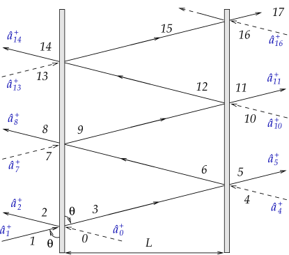
Figure 1: The Fabry-Perot interferometer. Each input/output mode is labelled with a number, starting with $0$. We associate to each input/output mode $l$ a field creation operator denoted by $\hat{a}^{\dagger}_{l}$.

Since the interesting case from a practical point of view is when the angle of incidence is almost normal ($\theta\to\pi/2$), we shall consider this scenario for the rest of the paper. In this case, our FP interferometer can be considered as having only four modes (ports) as depicted in Fig. 2 (see also the discussion in Appendix A). We can find the input-output operator transformations by various means. In Appendix A, they are obtained via a graphical method. The end results are

$$\hat{a}_{I}^{\dagger}=T_{fp}\hat{a}_{T}^{\dagger}+R_{fp}\hat{a}_{R}^{\dagger}$$ (2)

and

$$\hat{a}_{V}^{\dagger}=R_{fp}\hat{a}_{T}^{\dagger}+T_{fp}\hat{a}_{R}^{\dagger}$$ (3)

where $T_{fp}$ and, respectively, $R_{fp}$ are given by equations (30) and, respectively, (31).

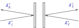
Figure 2: The creation field operators for a Fabry-Perot interferometer when $\theta\to\pi/2$. Input modes are labelled by $I$ and $V$, while output modes are labelled by $T$ and $R$. Each input/output mode has the corresponding creation operator attached to it.

By analyzing equations (2) and (3) one notes that these are actually the operator transformations of a beam splitter having frequency dependent transmissivity

$$T_{fp}\left(\omega\right)=\frac{T^{2}\text{e}^{i\omega t_{0}}}{1-R^{2}\text{e}^{i2\omega t_{0}}}$$ (4)

and reflectivity

$$R_{fp}\left(\omega\right)=R\frac{1+\text{e}^{i2\omega t_{0}}}{1-R^{2}\text{e}^{i2\omega t_{0}}}$$ (5)

coefficients. The probability of transmission and, respectively, reflection of a monochromatic beam of light of frequency $\omega$ is easily computed as

$$|{T_{fp}\left(\omega\right)}|^{2}=\frac{1}{1+\mathcal{F}^{2}\cos^{2}\left(\omega t_{0}\right)}$$ (6)

and

$$|{R_{fp}\left(\omega\right)}|^{2}=\frac{\mathcal{F}^{2}\cos^{2}\left(\omega t_{0}\right)}{1+\mathcal{F}^{2}\cos^{2}\left(\omega t_{0}\right)}$$ (7)

where we replaced $T$ and $R$ according to equation (1) and the cavity finesse was defined as $\mathcal{F}=2\sqrt{1-\varepsilon^{2}}/\varepsilon^{2}$. We note that we have $|{T_{fp}\left(\omega\right)}|^{2}+|{R_{fp}\left(\omega\right)}|^{2}=1$ and $T_{fp}\left(\omega\right)R_{fp}^{*}\left(\omega\right)+T_{fp}^{*}\left(\omega\right)R_{fp}\left(\omega\right)=0$ i.e. we have a $SU(2)$ symmetry, characteristic of linear lossless optical systems Yur86 ; Cam89 .

Therefore, the whole Fabry-Perot interferometer can be modelled as a simple beam splitter (see Fig. 3), with its transmissivity and reflectivity coefficients being heavily frequency dependent.

It is then expected that, similar to a beam splitter, the same classical and non-classical effects from quantum optics must be reproduced by a FP interferometer.

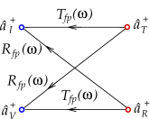
Figure 3: The Fabry-Perot interferometer can be also seen as a beam splitter with frequency-dependent $T_{fp}\left(\omega\right)$ and $R_{fp}\left(\omega\right)$ (transmission and reflection coefficients).

3 Antibunching with a Fabry-Perot interferometer in the case with monochromatic photons

The antibunching is a non-classical effect observed when two single-photon Fock states impinge simultaneously on the two inputs of a balanced ($50/50$) beam splitter HOM87 .

Since the Fabry-Perot interferometer is formally equivalent to a beam splitter (with frequency dependent transmissivity and reflectivity, as discussed before), using the $|1_{I}1_{V}\rangle$ input state should show this nonclassical effect at its output. Therefore, we apply the input state to a FP interferometer

$$|\psi_{in}\rangle=|1_{I}1_{V}\rangle=\hat{a}_{I}^{\dagger}\hat{a}_{V}^{\dagger}|0\rangle$$ (8)

where both input light quanta are supposed to be monochromatic of frequency $\omega$. Using again the input-output field operator transformation relations (2) and (3) takes us to the output state vector

$$|\psi_{out}\rangle=\left(T_{fp}\hat{a}_{T}^{\dagger}+R_{fp}\hat{a}_{R}^{\dagger}\right)\left(R_{fp}\hat{a}_{T}^{\dagger}+T_{fp}\hat{a}_{R}^{\dagger}\right)|0\rangle$$

$$=T_{fp}R_{fp}\left(|2_{T}0_{R}\rangle+|0_{T}2_{R}\rangle\right)+\left(T_{fp}^{2}+R_{fp}^{2}\right)|1_{T}1_{R}\rangle$$ (9)

We shall denote by $c_{HOM}\left(\varepsilon,\omega\right)=T_{fp}^{2}\left(\omega\right)+R_{fp}^{2}\left(\omega\right)$ and $P_{HOM}\left(\varepsilon,\omega\right)=|{c_{HOM}\left(\varepsilon,\omega\right)}|^{2}$ the amplitude, and, respectively, the probability of coincidence detection at the outputs $T$ and $R$ of the FP interferometer.

In order to obtain the antibunching effect, we impose the amplitude of the $|1_{T}1_{R}\rangle$ state to be zero. The condition $c_{HOM}\left(\omega\right)=0$ implies $\cos^{2}\left(\omega t_{0}\right)=\varepsilon^{4}/4\left(1-\varepsilon^{2}\right)$, an equation that can be readily solved yielding

$$\omega_{+/-}=\frac{1}{t_{0}}\arccos\left(\pm\frac{\varepsilon^{2}}{2\sqrt{1-\varepsilon^{2}}}\right)$$ (10)

This equation has solutions as long as $\varepsilon\leq\varepsilon_{0}$, where $\varepsilon_{0}=\sqrt{2\left(\sqrt{2}-1\right)}$. We could see $\varepsilon_{0}$ as the maximum value of the transmissivity of the individual mirrors, so that the FP interferometer can still exhibit the antibunching effect.

In practice, however, having $P_{HOM}\left(\varepsilon,\omega\right)$ below a certain value would be still satisfactory. In Fig. 4 we plot $P_{HOM}(\varepsilon,\omega)$ in respect with the transmissivity of individual mirrors ($\varepsilon$) and the phase variation ($\omega t_{0}/\pi$). The thick blue curve from Fig. 4 outlines the values $\varepsilon$ and $\omega$ for $P_{HOM}<0.01$.

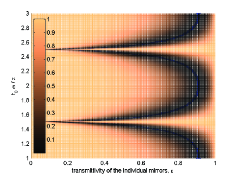
Figure 4: The antibunching factor $P_{HOM}=|{c_{HOM}}|^{2}$ versus the transmissivity of individual mirrors $\varepsilon$ and the phase variation $\omega t_{0}/\pi$. The blue thick curve corresponds to pairs $(\varepsilon,\omega)$ yielding $P_{HOM}(\varepsilon,\omega)\leq 0.01$.

Up until now, these results are equivalent to the ones obtained with a balanced beam splitter. The true interest in using a FP interferometer lies in the fact that the same effect can be obtained using photons of different colors.

We consider now two (monochromatic) photons of two different frequencies, $\omega_{s}$ and $\omega_{i}$. Therefore, the input state can be written as

$$|\psi_{in}\rangle=\iint{\text{d}\omega\text{d}\omega^{\prime}\zeta_{I}\left(\omega\right)\zeta_{\>V}\left(\omega^{\prime}\right)\hat{a}_{I}^{\dagger}\left(\omega\right)\hat{a}_{V}^{\dagger}\left(\omega^{\prime}\right)}|0\rangle$$ (11)

with $\zeta_{I}\left(\omega\right)=\delta\left(\omega-\omega_{s}\right)$ and $\zeta_{\>V}\left(\omega\right)=\delta\left(\omega-\omega_{i}\right)$. The frequency-dependent input-output creation operators now yield

$$\hat{a}_{I}^{\dagger}\left(\omega_{s}\right)=T_{fp}\left(\omega_{s}\right)\hat{a}_{T}^{\dagger}\left(\omega_{s}\right)+R_{fp}\left(\omega_{s}\right)\hat{a}_{R}^{\dagger}\left(\omega_{s}\right)$$ (12)

and

$$\hat{a}_{V}^{\dagger}\left(\omega_{i}\right)=R_{fp}\left(\omega_{i}\right)\hat{a}_{T}^{\dagger}\left(\omega_{i}\right)+T_{fp}\left(\omega_{i}\right)\hat{a}_{R}^{\dagger}\left(\omega_{i}\right)$$ (13)

The output state vector is obtained by considering the field operator transformations (12$-$13) on $|\psi_{in}\rangle$ from equation (11) and gives

$$|\psi_{out}\rangle=T_{fp}\left(\omega_{s}\right)R_{fp}\left(\omega_{i}\right)\hat{a}_{T}^{\dagger}\left(\omega_{s}\right)\hat{a}_{T}^{\dagger}\left(\omega_{i}\right)|0\rangle+$$

$$T_{fp}\left(\omega_{i}\right)R_{fp}\left(\omega_{s}\right)\hat{a}_{R}^{\dagger}\left(\omega_{s}\right)\hat{a}_{R}^{\dagger}\left(\omega_{i}\right)|0\rangle+$$

$$\left(T_{fp}\left(\omega_{s}\right)T_{fp}\left(\omega_{i}\right)\hat{a}_{T}^{\dagger}\left(\omega_{s}\right)\hat{a}_{R}^{\dagger}\left(\omega_{i}\right)\right.$$

$$\left.+R_{fp}\left(\omega_{s}\right)R_{fp}\left(\omega_{i}\right)\hat{a}_{T}^{\dagger}\left(\omega_{i}\right)\hat{a}_{R}^{\dagger}\left(\omega_{s}\right)\right)|0\rangle$$ (14)

Since the photon counters are typically frequency non-selective (at least in a small spectral range), a coincidence detection at the $T$ and $R$ outputs can be modelled as

$$c_{HOM}\left(\omega_{s},\omega_{i}\right)=\langle 0|\iint{\text{d}\omega\text{d}\omega^{\prime}\hat{a}_{T}\left(\omega\right)\hat{a}_{R}\left(\omega^{\prime}\right)}|\psi_{out}\rangle$$

$$=T_{fp}\left(\omega_{s}\right)T_{fp}\left(\omega_{i}\right)+R_{fp}\left(\omega_{s}\right)R_{fp}\left(\omega_{i}\right)$$ (15)

where we used the commutation relations Lou03

$$[\hat{a}_{l}\left(\omega\right),\hat{a}_{l}^{\dagger}\left(\omega^{\prime}\right)]=\delta\left(\omega-\omega^{\prime}\right)$$ (16)

for $l\in\{T,R\}$. The antibunching condition now reads $c_{HOM}\left(\omega_{s},\omega_{i}\right)=0$, leading to the constraint on $\omega_{s}$ and $\omega_{i}$:

$$\cos\left(\omega_{s}t_{0}\right)\cos\left(\omega_{i}t_{0}\right)=\frac{\varepsilon^{4}}{4\left(1-\varepsilon^{2}\right)}$$ (17)

Again, in a practical scenario, we might relax our constraints and, instead of imposing a zero amplitude for $c_{HOM}\left(\omega_{s},\omega_{i}\right)$, we could ask for a value of $P_{HOM}\left(\omega_{s},\omega_{i}\right)=|c_{HOM}\left(\omega_{s},\omega_{i}\right)|^{2}$ below a certain limit. The points $\left(\omega_{s},\omega_{i}\right)$ satisfying $P_{HOM}\left(\omega_{s},\omega_{i}\right)<0.01$ are plotted in Fig. 5 for three different values of $\varepsilon$.

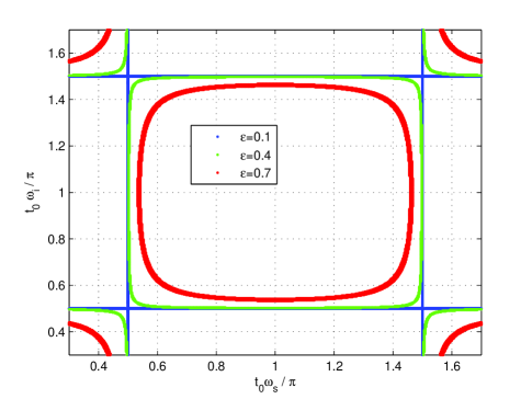
Figure 5: The pairs of frequencies $\left(\omega_{s},\omega_{i}\right)$ satisfying $P_{HOM}\left(\omega_{s},\omega_{i}\right)<0.01$. The thick red curve corresponds to $\varepsilon=0.7$, the green one corresponds to $\varepsilon=0.4$ and the blue curve corresponds to $\varepsilon=0.1$.

In Appendix B we discuss what changes implies the more realistic assumption that the signal and idler photons originate from a SPDC process.

4 Antibunching with a Fabry-Perot interferometer in the case of non-monochromatic photons

We extend now the previous analysis to non-monochromatic photon wave packets Blo90 ; Cam90 . The input state can be expressed as

$$|\psi_{in}\rangle=\iint{\text{d}\omega\text{d}\omega^{\prime}\zeta\left(\omega,\omega^{\prime}\right)\hat{a}_{I}^{\dagger}\left(\omega\right)\hat{a}_{V}^{\dagger}\left(\omega^{\prime}\right)}|0\rangle$$ (18)

where $\zeta\left(\omega,\omega^{\prime}\right)$ is the bi-photon wave packet and it is normalized via $\iint{|\zeta\left(\omega,\omega^{\prime}\right)|^{2}\text{d}\omega\text{d}\omega^{\prime}}=1$. The output positive frequency electric field operators have to be extended to

$$\hat{E}_{l}^{(+)}\left(t\right)=\frac{1}{\sqrt{2\pi}}\int{\text{d}\omega\text{e}^{-i\omega{t}}\hat{a}_{l}\left(\omega\right)}$$ (19)

where $l\in\{T,R\}$. We shall be interested in the second order correlation function Lou03 ; Man95

$$G^{(2)}\left(t,t+\tau\right)=\langle\psi_{out}|\hat{E}_{T}^{(-)}\left(t\right)\hat{E}_{R}^{(-)}\left(t+\tau\right)$$

$$\hat{E}_{R}^{(+)}\left(t+\tau\right)\hat{E}_{T}^{(+)}\left(t\right)|\psi_{out}\rangle$$ (20)

where $\hat{E}_{l}^{(-)}\left(t\right)=[\hat{E}_{l}^{(+)}\left(t\right)]^{\dagger}$ and $t$ ($t+\tau$) denotes the detection time at the output $T$ ($R$). We will use the Schrödinger picture therefore we shall evolve $|\psi_{in}\rangle$ to $|\psi_{out}\rangle$. Using again the field operator transformations (2) and (3) obtaining the output state vector

$$|\psi_{out}\rangle=\iint{\text{d}\omega\text{d}\omega^{\prime}}\left(T_{fp}\left(\omega\right)\hat{a}_{T}^{\dagger}\left(\omega\right)+R_{fp}\left(\omega\right)\hat{a}_{R}^{\dagger}\left(\omega\right)\right)$$

$$\times\left(R_{fp}\left(\omega^{\prime}\right)\hat{a}_{T}^{\dagger}\left(\omega^{\prime}\right)+T_{fp}\left(\omega^{\prime}\right)\hat{a}_{R}^{\dagger}\left(\omega^{\prime}\right)\right)\zeta\left(\omega,\omega^{\prime}\right)|0\rangle\quad$$ (21)

Combining now equations (19), (4) and (4), after some computations, one ends up with

$$G^{(2)}\left(t,t+\tau\right)=\frac{1}{2\pi}\bigg{|}\iint{\text{d}\omega\text{d}\omega^{\prime}\text{e}^{-i\omega{t}}\text{e}^{-i\omega^{\prime}\left(t+\tau\right)}}\qquad$$

$$\times\left(T_{fp}\left(\omega\right)T_{fp}\left(\omega^{\prime}\right)+R_{fp}\left(\omega\right)R_{fp}\left(\omega^{\prime}\right)\right)\zeta\left(\omega,\omega^{\prime}\right)\bigg{|}^{2}$$ (22)

where we used again the commutation relations (16). If we make the simplifying assumption that the signal and idler frequencies are not frequency correlated i.e. we have $\zeta\left(\omega,\omega^{\prime}\right)=\zeta_{0}\left(\omega\right)\zeta_{1}\left(\omega^{\prime}\right)$, equation (4) simplifies to

$$G^{(2)}\left(t,t+\tau\right)=|\zeta_{0}^{T}\left(t\right)\zeta_{1}^{T}\left(t+\tau\right)+\zeta_{0}^{R}\left(t+\tau\right)\zeta_{1}^{R}\left(t\right)|^{2}\quad$$ (23)

where we have the inverse Fourier transforms

$$\zeta_{m}^{T}\left(t\right)=\frac{1}{\sqrt{2\pi}}\int{\text{d}\omega\text{e}^{-i\omega{t}}T_{fp}\left(\omega\right)\zeta_{m}\left(\omega\right)}$$ (24)

and

$$\zeta_{m}^{R}\left(t\right)=\frac{1}{\sqrt{2\pi}}\int{\text{d}\omega\text{e}^{-i\omega{t}}R_{fp}\left(\omega\right)\zeta_{m}\left(\omega\right)}$$ (25)

with $m\in\{0,1\}$. To the author’s best knowledge, there is no closed-form solution to these Fourier integrals. However, one can easily check that if $\zeta_{0}\left(\omega\right)\to\delta\left(\omega-\omega_{s}\right)$ and $\zeta_{1}\left(\omega^{\prime}\right)\to\delta\left(\omega^{\prime}-\omega_{i}\right)$ equation (4) migrates into

$$G^{(2)}\sim|T_{fp}\left(\omega_{s}\right)T_{fp}\left(\omega_{i}\right)+R_{fp}\left(\omega_{s}\right)R_{fp}\left(\omega_{i}\right)|^{2}$$ (26)

If $\omega_{s}$ and $\omega_{i}$ obey equation (17), then the antibunching effect is assured. If one assumes the SPDC-like frequency correlation, $\zeta\left(\omega,\omega^{\prime}\right)\to\delta\left(\omega-\omega_{s}\right)\delta\left(\omega^{\prime}-\omega_{p}+\omega_{s}\right)$ the discussion from Appendix B still holds.

5 Conclusions

In this paper we started from the full quantum optical description of a Fabry-Perot interferometer and showed that it can be modelled through a beam splitter having heavily frequency-dependent transmission and reflection coefficients.

Owing to this model, the antibunching effect, well-known for beam splitters has been predicted for the Fabry-Perot interferometer, too. However, even different frequency photons can show this effect, this being in contrast with the normal antibunching. Monochromatic, as well as non-monochromatic input light was considered.

Appendix A The computation of the field operator transformations in a FP interferometer

In the following we will employ the graphical method introduced in Ata14b . Beam splitters will be depicted by the butterfly-like structure and delays will simply add a $\text{e}^{i\varphi}$ factor. The graphical representation of the Fabry-Perot interferometer is detailed in Fig. 6. Each crossing of a highly-reflecting mirror is modelled by a beam splitter (having the transmission and reflection coefficients $T$ and, respectively, $R$) and each passage inside the cavity yields an extra factor of $\text{e}^{i\varphi}$ where $\varphi=kL$ and $k$ is the wavenumber of the (monochromatic) light that illuminates the interferometer.

Figure 6: The graphical description of a Fabry-Perot interferometer for light incident at an arbitrary angle. Each passage of the beam through the highly reflecting mirrors is modelled with a beam splitter. The labelling was done in accordance to Fig. 1.

It is not difficult to find the expression of the input creation operator $\hat{a}_{1}^{\dagger}$ in respect with the output ones. We can differentiate between transmission type creation operators ($\hat{a}_{5}^{\dagger}$, $\hat{a}_{11}^{\dagger}$, $\hat{a}_{17}^{\dagger}$ $\ldots$) and reflection type operators ($\hat{a}_{2}^{\dagger}$, $\hat{a}_{8}^{\dagger}$, $\hat{a}_{14}^{\dagger}$ $\ldots$). Adding up all these contributions, one ends up with

$$\hat{a}_{1}^{\dagger}=T^{2}\text{e}^{i\varphi}\left(\hat{a}_{5}^{\dagger}+R^{2}\text{e}^{i2\varphi}\hat{a}_{11}^{\dagger}+R^{4}\text{e}^{i4\varphi}\hat{a}_{17}^{\dagger}+\ldots\right)$$

$$+R\left(\hat{a}_{2}^{\dagger}+T^{2}\text{e}^{i2\varphi}\hat{a}_{8}^{\dagger}+T^{2}R^{2}\text{e}^{i4\varphi}\hat{a}_{14}^{\dagger}+\ldots\right)$$ (27)

As discussed before, the interesting case from a practical point of view is when the angle $\theta$ tends to $\pi/2$. The many inputs and outputs tend to group together in the following way: the inputs ($\hat{a}_{1}^{\dagger}$, $\hat{a}_{7}^{\dagger}$, $\hat{a}_{13}^{\dagger}$ $\ldots$) become indistinguishable and we relabel them as a single input $I$, whose creation operator will be denoted by $\hat{a}_{I}^{\dagger}$. Similarly the reflected outputs ($\hat{a}_{2}^{\dagger}$, $\hat{a}_{8}^{\dagger}$, $\hat{a}_{14}^{\dagger}$ $\ldots$) become also indistinguishable and will be denoted by $\hat{a}_{R}^{\dagger}$. The same logic applies in regrouping the appropriate transmission operators ($\hat{a}_{5}^{\dagger}$, $\hat{a}_{8}$, $\hat{a}_{11}^{\dagger}$, $\hat{a}_{17}^{\dagger}$ $\ldots$) into $\hat{a}_{T}^{\dagger}$. The “dark” ports ($\hat{a}_{0}^{\dagger}$, $\hat{a}_{4}^{\dagger}$, $\hat{a}_{10}^{\dagger}$, $\hat{a}_{16}^{\dagger}$ $\ldots$) are grouped into the “vacuum” port $\hat{a}_{V}^{\dagger}$ (see Fig. 2). Now equation (A) takes the much simpler form

$$\hat{a}_{I}^{\dagger}=T^{2}\text{e}^{i\varphi}\left(1+R^{2}\text{e}^{i2\varphi}+R^{4}\text{e}^{i4\varphi}+\ldots\right)\hat{a}_{T}^{\dagger}$$

$$+R\left(1+T^{2}\text{e}^{i2\varphi}+T^{2}R^{2}\text{e}^{i4\varphi}+\ldots\right)\hat{a}_{R}^{\dagger}$$ (28)

Since we have now two trivial geometric series and $|{R}|<1$, equation (A) can be written in the rather simple form

$$\hat{a}_{I}^{\dagger}=\frac{T^{2}\text{e}^{i\varphi}}{1-R^{2}\text{e}^{i2\varphi}}\hat{a}_{T}^{\dagger}+R\left(1+\frac{T^{2}\text{e}^{i2\varphi}}{1-R^{2}\text{e}^{i2\varphi}}\right)\hat{a}_{R}^{\dagger}$$ (29)

We could define the transmission

$$T_{fp}=\frac{T^{2}\text{e}^{i\varphi}}{1-R^{2}\text{e}^{i2\varphi}}$$ (30)

and reflection

$$R_{fp}=R\left(1+\frac{T^{2}\text{e}^{i2\varphi}}{1-R^{2}\text{e}^{i2\varphi}}\right)$$ (31)

coefficients of the FP interferometer allowing the easy writing of the field operator transformation given by equation (2). Similar arguments allow one to write $\hat{a}_{V}^{\dagger}$ in respect with $\hat{a}_{T}^{\dagger}$ and $\hat{a}_{R}^{\dagger}$, as done in equation (3).

The regrouping of input and output field operators that became indistinguishable allows a much simpler graphical representation of the FP interferometer, as depicted in Fig. 7.

The infinite series of beam splitters from Fig. 6 was replaced by a loop, having the nodes $B$, $C$, $D$ and $E$ in Fig. 7. The meaning of the loop is that besides the direct path, there is a possibility to loop ones, twice and so forth. For example, in Fig. 7, the direct path from $\hat{a}_{T}^{\dagger}$ to $\hat{a}_{I}^{\dagger}$ took simply a factor of $\text{e}^{i\varphi}$ (besides the $T^{2}$ factor caused by elements outside of the loop). Looping ones implies, besides $\text{e}^{i\varphi}$, a supplementary factor of $R^{2}\text{e}^{i2\varphi}$. Looping twice implies a supplementary factor of $R^{4}\text{e}^{i4\varphi}$ and so forth. This is the geometric series ($1+R^{2}\text{e}^{i2\varphi}+R^{4}\text{e}^{i4\varphi}+\ldots$) we found before and it trivially yields $1/(1-R^{2}\text{e}^{i2\varphi})$. In the end, from the recursive graphical method we obtain $T^{2}\text{e}^{i\varphi}/(1-R^{2}\text{e}^{i2\varphi})$, a result identical to equation (30).

Therefore, as a rule, in the graph from Fig. 7, every input-output path having a common segment with this loop must take a supplementary factor of $1/(1-R^{2}\text{e}^{i2\varphi})$.

For example, the input creation operator $\hat{a}_{I}^{\dagger}$ can be reached from the output port $\hat{a}_{R}^{\dagger}$ through the reflection coefficient of the input beam splitter yielding a factor $R$ (and touching no loop). There is a second contribution from $\hat{a}_{R}^{\dagger}$ to $\hat{a}_{I}^{\dagger}$: transmission $T$ from the first (left) beam splitter, a factor of $\text{e}^{i\varphi}$, a $R$ (from the second i.e. right beam splitter), another factor of $\text{e}^{i\varphi}$ and finally a factor of $T$ to $\hat{a}_{I}^{\dagger}$. This path has common segments with the loop, therefore it also takes the factor $1/(1-R^{2}\text{e}^{i2\varphi})$. Adding up the two possible routes gives $R+RT^{2}\text{e}^{i2\varphi}/(1-R^{2}\text{e}^{i2\varphi})$ and we found straight away the result from equation (31).

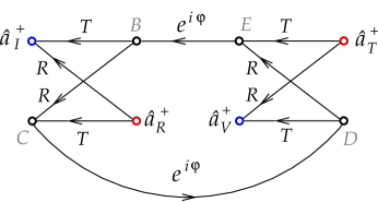
Figure 7: The graphical description of a Fabry-Perot interferometer in the recursive form when light impinges at a normal angle. The blue circles denote the input ports while the red ones denote the output ports. Every path having a common segment with the loop $B-C-D-E$ gains a factor of $1/(1-R^{2}\text{e}^{i2\varphi})$.

Appendix B The antibunching condition with photons originating in a SPDC process

In the SPDC process, the signal and idler frequencies are bound by the relation $\omega_{p}=\omega_{s}+\omega_{i}$ where $\omega_{p}$ denotes the pump frequency. This constraint modifies equation (17) and takes us to a single variable (say $\omega_{s}$) yielding

$$\alpha_{p}\cos\left(2\omega_{s}t_{0}\right)+\sqrt{1-\alpha_{p}^{2}}\sin\left(2\omega_{s}t_{0}\right)=\beta_{\varepsilon}-\alpha_{p}$$ (32)

where we denoted $\alpha_{p}=\cos\left(\omega_{p}t_{0}\right)$ and $\beta_{\varepsilon}=\varepsilon^{4}/2\left(1-\varepsilon^{2}\right)$. Using well-known trigonometric identities, we transform the sines and cosines into $\tan\left(\omega_{s}t_{0}\right)$ and have

$$\beta_{\varepsilon}\tan^{2}\left(\omega_{s}t_{0}\right)-2\sqrt{1-\alpha_{p}^{2}}\tan\left(\omega_{s}t_{0}\right)+\beta_{\varepsilon}-2\alpha_{p}=0\quad$$ (33)

This second order equation in $\tan\left(\omega_{s}t_{0}\right)$ yields two solutions

$$\tan\left(\omega_{s}t_{0}\right)|_{+/-}=\frac{\sqrt{1-\alpha_{p}^{2}}\pm\sqrt{1-\alpha_{p}^{2}-\beta^{2}_{\varepsilon}+2\alpha_{p}\beta_{\varepsilon}}}{\beta_{\varepsilon}}\quad$$ (34)

as long as the quantity under the square root is not negative. This constraint imposes

$$\alpha_{p}^{2}-2\alpha_{p}\beta_{\varepsilon}+\beta^{2}_{\varepsilon}-1\leq 0$$ (35)

This can happen only if $\alpha_{p}$ is

$$\beta_{\varepsilon}-1\leq\alpha_{p}\leq\beta_{\varepsilon}+1$$ (36)

The second inequality is always satisfied since $\beta_{\varepsilon}\geq 0$, therefore we are left with

$$\frac{\varepsilon^{4}}{2\left(1-\varepsilon^{2}\right)}-1\leq\cos\left(\omega_{p}t_{0}\right)$$ (37)

This relation puts constraints on the values of $t_{0}$, $\omega_{p}$ and $\varepsilon$ in order to make possible the antibunching effect at the signal frequency $\omega_{s}$.

References

- (1) C. Fabry, A. Perot, Ann. de Chim. et de Phys. 16, 115 (1899)
- (2) N. Hodgson, H. Weber, Optical Resonators: Fundamentals, Advanced Concepts, and Applications (Springer-Verlag, Berlin, 1997)
- (3) K. S. Thorne, Rev. Mod. Phys. 52, 285 (1980)
- (4) S. Kuhr et al. Appl. Phys. Lett. 90, 164101 (2007)
- (5) D Hunger et al. New J. Phys. 12 065038 (2010)
- (6) M. J. Lawrence et al. J. Opt. Soc. Am. B 16, 523 (1999)
- (7) H. Rohde, J. Eschner, F. Schmidt-Kaler, R. Blatt, JOSA B 19, 1425 (2002)
- (8) F. Fratini et al., PRL 113, 243601 (2014)
- (9) G. Hétet et al., PRL 107, 133002 (2011)
- (10) Bh. Srivathsan et al. PRL 113, 163601 (2014)
- (11) D. Bouwmeester, A. Ekert, A. Zeilinger (Eds.), The Physics of Quantum Information, (Springer 2000)
- (12) Y. Sun, arXiv:1412.3867
- (13) D. C. Burnham, D. L. Weinberg, Phys. Rev. Lett. 25, 84 (1970)
- (14) D. N. Klyshko, Sov. Phys. JETP Lett. 6, 23 (1967)
- (15) C. Hong, Z. Ou, L. Mandel, Phys. Rev. Lett. 59, 18 (1987)
- (16) M. Ley, R. Loudon, J. Mod. Opt. 34, 227 (1987)
- (17) B. Yurke, S. McCall, J. Klauder, Phys. Rev. A 33, 4033 (1986)
- (18) R. Campos, B. Saleh, M. Teich, Phys. Rev. A 40, 1371 (1989)
- (19) S. Ataman, Eur. Phys. J. D 68, 288 (2014)
- (20) S. Ataman, Eur. Phys. J. D 69, 44 (2015)
- (21) R. Loudon, The quantum theory of light, (Oxford University Press, Third Edition, 2003)
- (22) K. Blow, R. Loudon, S. Phoenix, T. Shepherd, Phys. Rev. A 42, 4102 (1990).
- (23) R. Campos, B. Saleh, M. Teich, Phys. Rev. A 42, 4127 (1990)
- (24) L. Mandel, E. Wolf, Optical Coherence and Quantum Optics, (Cambridge, 1995)