A hybrid algorithm for Bayesian network structure learning
with application to multi-label learning
Abstract
We present a novel hybrid algorithm for Bayesian network structure learning, called H2PC. It first reconstructs the skeleton of a Bayesian network and then performs a Bayesian-scoring greedy hill-climbing search to orient the edges. The algorithm is based on divide-and-conquer constraint-based subroutines to learn the local structure around a target variable. We conduct two series of experimental comparisons of H2PC against Max-Min Hill-Climbing (MMHC), which is currently the most powerful state-of-the-art algorithm for Bayesian network structure learning. First, we use eight well-known Bayesian network benchmarks with various data sizes to assess the quality of the learned structure returned by the algorithms. Our extensive experiments show that H2PC outperforms MMHC in terms of goodness of fit to new data and quality of the network structure with respect to the true dependence structure of the data. Second, we investigate H2PC’s ability to solve the multi-label learning problem. We provide theoretical results to characterize and identify graphically the so-called minimal label powersets that appear as irreducible factors in the joint distribution under the faithfulness condition. The multi-label learning problem is then decomposed into a series of multi-class classification problems, where each multi-class variable encodes a label powerset. H2PC is shown to compare favorably to MMHC in terms of global classification accuracy over ten multi-label data sets covering different application domains. Overall, our experiments support the conclusions that local structural learning with H2PC in the form of local neighborhood induction is a theoretically well-motivated and empirically effective learning framework that is well suited to multi-label learning. The source code (in R) of H2PC as well as all data sets used for the empirical tests are publicly available.
keywords:
Bayesian networks , Multi-label learning , Markov boundary , Feature subset selection.1 Introduction
A Bayesian network (BN) is a probabilistic model formed by a structure and parameters. The structure of a BN is a directed acyclic graph (DAG), whilst its parameters are conditional probability distributions associated with the variables in the model. The problem of finding the DAG that encodes the conditional independencies present in the data attracted a great deal of interest over the last years (Rodrigues de Morais & Aussem, 2010a; Scutari, 2010; Scutari & Brogini, 2012; Kojima et al., 2010; Perrier et al., 2008; Villanueva & Maciel, 2012; Peña, 2012; Gasse et al., 2012). The inferred DAG is very useful for many applications, including feature selection (Aliferis et al., 2010; Peña et al., 2007; Rodrigues de Morais & Aussem, 2010b), causal relationships inference from observational data (Ellis & Wong, 2008; Aliferis et al., 2010; Aussem et al., 2012, 2010; Prestat et al., 2013; Cawley, 2008; Brown & Tsamardinos, 2008) and more recently multi-label learning (Dembczyński et al., 2012; Zhang & Zhang, 2010; Guo & Gu, 2011).
Ideally the DAG should coincide with the dependence structure of the global distribution, or it should at least identify a distribution as close as possible to the correct one in the probability space. This step, called structure learning, is similar in approaches and terminology to model selection procedures for classical statistical models. Basically, constraint-based (CB) learning methods systematically check the data for conditional independence relationships and use them as constraints to construct a partially oriented graph representative of a BN equivalence class, whilst search-and-score (SS) methods make use of a goodness-of-fit score function for evaluating graphical structures with regard to the data set. Hybrid methods attempt to get the best of both worlds: they learn a skeleton with a CB approach and constrain on the DAGs considered during the SS phase.
In this study, we present a novel hybrid algorithm for Bayesian network structure learning, called H2PC111A first version of HP2C without FDR control has been discussed in a paper that appeared in the Proceedings of ECML-PKDD, pages 58-73, 2012.. It first reconstructs the skeleton of a Bayesian network and then performs a Bayesian-scoring greedy hill-climbing search to orient the edges. The algorithm is based on divide-and-conquer constraint-based subroutines to learn the local structure around a target variable. HPC may be thought of as a way to compensate for the large number of false negatives at the output of the weak PC learner, by performing extra computations. As this may arise at the expense of the number of false positives, we control the expected proportion of false discoveries (i.e. false positive nodes) among all the discoveries made in . We use a modification of the Incremental association Markov boundary algorithm (IAMB), initially developed by Tsamardinos et al. in (Tsamardinos et al., 2003) and later modified by Jose Peña in (Peña, 2008) to control the FDR of edges when learning Bayesian network models. HPC scales to thousands of variables and can deal with many fewer samples (). To illustrate its performance by means of empirical evidence, we conduct two series of experimental comparisons of H2PC against Max-Min Hill-Climbing (MMHC), which is currently the most powerful state-of-the-art algorithm for BN structure learning (Tsamardinos et al., 2006), using well-known BN benchmarks with various data sizes, to assess the goodness of fit to new data as well as the quality of the network structure with respect to the true dependence structure of the data.
We then address a real application of H2PC where the true dependence structure is unknown. More specifically, we investigate H2PC’s ability to encode the joint distribution of the label set conditioned on the input features in the multi-label classification (MLC) problem. Many challenging applications, such as photo and video annotation and web page categorization, can benefit from being formulated as MLC tasks with large number of categories (Dembczyński et al., 2012; Read et al., 2009; Madjarov et al., 2012; Kocev et al., 2007; Tsoumakas et al., 2010b). Recent research in MLC focuses on the exploitation of the label conditional dependency in order to better predict the label combination for each example. We show that local BN structure discovery methods offer an elegant and powerful approach to solve this problem. We establish two theorems (Theorem 6 and 7) linking the concepts of marginal Markov boundaries, joint Markov boundaries and so-called label powersets under the faithfulness assumption. These Theorems offer a simple guideline to characterize graphically : i) the minimal label powerset decomposition, (i.e. into minimal subsets such that ), and ii) the minimal subset of features, w.r.t an Information Theory criterion, needed to predict each label powerset, thereby reducing the input space and the computational burden of the multi-label classification. To solve the MLC problem with BNs, the DAG obtained from the data plays a pivotal role. So in this second series of experiments, we assess the comparative ability of H2PC and MMHC to encode the label dependency structure by means of an indirect goodness of fit indicator, namely the loss function, which makes sense in the MLC context.
The rest of the paper is organized as follows: In the Section 2, we review the theory of BN and discuss the main BN structure learning strategies. We then present the H2PC algorithm in details in Section 3. Section 4 evaluates our proposed method and shows results for several tasks involving artificial data sampled from known BNs. Then we report, in Section 5, on our experiments on real-world data sets in a multi-label learning context so as to provide empirical support for the proposed methodology. The main theoretical results appear formally as two theorems (Theorem 8 and 9) in Section 5. Their proofs are established in the Appendix. Finally, Section 6 raises several issues for future work and we conclude in Section 7 with a summary of our contribution.
2 Preliminaries
We define next some key concepts used along the paper and state some results that will support our analysis. In this paper, upper-case letters in italics denote random variables (e.g., ) and lower-case letters in italics denote their values (e.g., ). Upper-case bold letters denote random variable sets (e.g., ) and lower-case bold letters denote their values (e.g., ). We denote by the conditional independence between and given the set of variables . To keep the notation uncluttered, we use to denote .
2.1 Bayesian networks
Formally, a BN is a tuple , where is a directed acyclic graph (DAG) with nodes representing the random variables and a joint probability distribution in . In addition, and must satisfy the Markov condition: every variable, , is independent of any subset of its non-descendant variables conditioned on the set of its parents, denoted by . From the Markov condition, it is easy to prove (Neapolitan, 2004) that the joint probability distribution on the variables in can be factored as follows :
| (1) |
Equation 1 allows a parsimonious decomposition of the joint distribution . It enables us to reduce the problem of determining a huge number of probability values to that of determining relatively few.
A BN structure entails a set of conditional independence assumptions. They can all be identified by the d-separation criterion (Pearl, 1988). We use to denote the assertion that is d-separated from given in . Formally, is true when for every undirected path in between and , there exists a node in the path such that either (1) does not have two parents in the path and , or (2) has two parents in the path and neither nor its descendants is in . If is a BN, if . The converse does not necessarily hold. We say that satisfies the faithfulness condition if the d-separations in identify all and only the conditional independencies in , i.e., iff .
A Markov blanket of is any set of variables such that is conditionally independent of all the remaining variables given . By extension, a Markov blanket of in guarantees that , and that is conditionally independent of the remaining variables in , given . A Markov boundary, , of is any Markov blanket such that none of its proper subsets is a Markov blanket of .
We denote by , the set of parents and children of in , and by , the set of spouses of in . The spouses of are the variables that have common children with . These sets are unique for all , such that satisfies the faithfulness condition and so we will drop the superscript . We denote by , the set that d-separates from the (implicit) target .
Theorem 1.
Suppose satisfies the faithfulness condition. Then and are not adjacent in iff such that . Moreover, .
A proof can be found for instance in (Neapolitan, 2004).
Two graphs are said equivalent iff they encode the same set of conditional independencies via the d-separation criterion. The equivalence class of a DAG is a set of DAGs that are equivalent to . The next result showed by (Pearl, 1988), establishes that equivalent graphs have the same undirected graph but might disagree on the direction of some of the arcs.
Theorem 2.
Two DAGs are equivalent iff they have the same underlying undirected graph and the same set of v-structures (i.e. converging edges into the same node, such as ).
Moreover, an equivalence class of network structures can be uniquely represented by a partially directed DAG (PDAG), also called a DAG pattern. The DAG pattern is defined as the graph that has the same links as the DAGs in the equivalence class and has oriented all and only the edges common to the DAGs in the equivalence class. A structure learning algorithm from data is said to be correct (or sound) if it returns the correct DAG pattern (or a DAG in the correct equivalence class) under the assumptions that the independence tests are reliable and that the learning database is a sample from a distribution faithful to a DAG , The (ideal) assumption that the independence tests are reliable means that they decide (in)dependence iff the (in)dependence holds in .
2.2 Conditional independence properties
Theorem 3.
Let and denote four mutually disjoint subsets of . Any probability distribution satisfies the following four properties: Symmetry , Decomposition, , Weak Union and Contraction, .
Theorem 4.
If is strictly positive, then satisfies the previous four properties plus the Intersection property . Additionally, each has a unique Markov boundary,
Theorem 5.
If is faithful to a DAG , then satisfies the previous five properties plus the Composition property and the local Markov property for each , where denotes the non-descendants of in .
2.3 Structure learning strategies
The number of DAGs, , is super-exponential in the number of random variables in the domain and the problem of learning the most probable a posteriori BN from data is worst-case NP-hard (Chickering et al., 2004). One needs to resort to heuristical methods in order to be able to solve very large problems effectively.
Both CB and SS heuristic approaches have advantages and disadvantages. CB approaches are relatively quick, deterministic, and have a well defined stopping criterion; however, they rely on an arbitrary significance level to test for independence, and they can be unstable in the sense that an error early on in the search can have a cascading effect that causes many errors to be present in the final graph. SS approaches have the advantage of being able to flexibly incorporate users’ background knowledge in the form of prior probabilities over the structures and are also capable of dealing with incomplete records in the database (e.g. EM technique). Although SS methods are favored in practice when dealing with small dimensional data sets, they are slow to converge and the computational complexity often prevents us from finding optimal BN structures (Perrier et al., 2008; Kojima et al., 2010). With currently available exact algorithms (Koivisto & Sood, 2004; Silander & Myllymäki, 2006; Cussens & Bartlett, 2013; Studený & Haws, 2014) and a decomposable score like BDeu, the computational complexity remains exponential, and therefore, such algorithms are intractable for BNs with more than around 30 vertices on current workstations. For larger sets of variables the computational burden becomes prohibitive and restrictions about the structure have to be imposed, such as a limit on the size of the parent sets. With this in mind, the ability to restrict the search locally around the target variable is a key advantage of CB methods over SS methods. They are able to construct a local graph around the target node without having to construct the whole BN first, hence their scalability (Peña et al., 2007; Rodrigues de Morais & Aussem, 2010b, a; Tsamardinos et al., 2006; Peña, 2008).
With a view to balancing the computation cost with the desired accuracy of the estimates, several hybrid methods have been proposed recently. Tsamardinos et al. proposed in (Tsamardinos et al., 2006) the Min-Max Hill Climbing (MMHC) algorithm and conducted one of the most extensive empirical comparison performed in recent years showing that MMHC was the fastest and the most accurate method in terms of structural error based on the structural hamming distance. More specifically, MMHC outperformed both in terms of time efficiency and quality of reconstruction the PC (Spirtes et al., 2000), the Sparse Candidate (Friedman et al., 1999b), the Three Phase Dependency Analysis (Cheng et al., 2002), the Optimal Reinsertion (Moore & Wong, 2003), the Greedy Equivalence Search (Chickering, 2002), and the Greedy Hill-Climbing Search on a variety of networks, sample sizes, and parameter values. Although MMHC is rather heuristic by nature (it returns a local optimum of the score function), it is currently considered as the most powerful state-of-the-art algorithm for BN structure learning capable of dealing with thousands of nodes in reasonable time.
In order to enhance its performance on small dimensional data sets, Perrier et al. proposed in (Perrier et al., 2008) a hybrid algorithm that can learn an optimal BN (i.e., it converges to the true model in the sample limit) when an undirected graph is given as a structural constraint. They defined this undirected graph as a super-structure (i.e., every DAG considered in the SS phase is compelled to be a subgraph of the super-structure). This algorithm can learn optimal BNs containing up to 50 vertices when the average degree of the super-structure is around two, that is, a sparse structural constraint is assumed. To extend its feasibility to BN with a few hundred of vertices and an average degree up to four, Kojima et al. proposed in (Kojima et al., 2010) to divide the super-structure into several clusters and perform an optimal search on each of them in order to scale up to larger networks. Despite interesting improvements in terms of score and structural hamming distance on several benchmark BNs, they report running times about times longer than MMHC on average, which is still prohibitive.
Therefore, there is great deal of interest in hybrid methods capable of improving the structural accuracy of both CB and SS methods on graphs containing up to thousands of vertices. However, they make the strong assumption that the skeleton (also called super-structure) contains at least the edges of the true network and as small as possible extra edges. While controlling the false discovery rate (i.e., false extra edges) in BN learning has attracted some attention recently (Armen & Tsamardinos, 2011; Peña, 2008; Tsamardinos & Brown, 2008), to our knowledge, there is no work on controlling actively the rate of false-negative errors (i.e., false missing edges).
2.4 Constraint-based structure learning
Before introducing the H2PC algorithm, we discuss the general idea behind CB methods. The induction of local or global BN structures is handled by CB methods through the identification of local neighborhoods (i.e., ), hence their scalability to very high dimensional data sets. CB methods systematically check the data for conditional independence relationships in order to infer a target’s neighborhood. Typically, the algorithms run either a or a independence test when the data set is discrete and a Fisher’s Z test when it is continuous in order to decide on dependence or independence, that is, upon the rejection or acceptance of the null hypothesis of conditional independence. Since we are limiting ourselves to discrete data, both the global and the local distributions are assumed to be multinomial, and the latter are represented as conditional probability tables. Conditional independence tests and network scores for discrete data are functions of these conditional probability tables through the observed frequencies for the random variables and and all the configurations of the levels of the conditioning variables . We use as shorthand for the marginal and similarly for and . We use a classic conditional independence test based on the mutual information. The mutual information is an information-theoretic distance measure defined as
It is proportional to the log-likelihood ratio test (they differ by a 2n factor, where n is the sample size). The asymptotic null distribution is with degrees of freedom. For a detailed analysis of their properties we refer the reader to (Agresti, 2002). The main limitation of this test is the rate of convergence to its limiting distribution, which is particularly problematic when dealing with small samples and sparse contingency tables. The decision of accepting or rejecting the null hypothesis depends implicitly upon the degree of freedom which increases exponentially with the number of variables in the conditional set. Several heuristic solutions have emerged in the literature (Spirtes et al., 2000; Rodrigues de Morais & Aussem, 2010a; Tsamardinos et al., 2006; Tsamardinos & Borboudakis, 2010) to overcome some shortcomings of the asymptotic tests. In this study we use the two following heuristics that are used in MMHC. First, we do not perform and assume independence if there are not enough samples to achieve large enough power. We require that the average sample per count is above a user defined parameter, equal to 5, as in (Tsamardinos et al., 2006). This heuristic is called the power rule. Second, we consider as structural zero either case or . For example, if , we consider y as a structurally forbidden value for Y when Z = z and we reduce R by 1 (as if we had one column less in the contingency table where Z = z). This is known as the degrees of freedom adjustment heuristic.
3 The H2PC algorithm
In this section, we present our hybrid algorithm for Bayesian network structure learning, called Hybrid HPC (H2PC). It first reconstructs the skeleton of a Bayesian network and then performs a Bayesian-scoring greedy hill-climbing search to filter and orient the edges. It is based on a CB subroutine called HPC to learn the parents and children of a single variable. So, we shall discuss HPC first and then move to H2PC.
3.1 Parents and Children Discovery
HPC (Algorithm 1) can be viewed as an ensemble method for combining many weak PC learners in an attempt to produce a stronger PC learner. HPC is based on three subroutines: Data-Efficient Parents and Children Superset (DE-PCS), Data-Efficient Spouses Superset (DE-SPS), and Incremental Association Parents and Children with false discovery rate control (FDR-IAPC), a weak PC learner based on FDR-IAMB (Peña, 2008) that requires little computation. HPC receives a target node T, a data set and a set of variables U as input and returns an estimation of . It is hybrid in that it combines the benefits of incremental and divide-and-conquer methods. The procedure starts by extracting a superset of (line 1) and a superset of (line 2) with a severe restriction on the maximum conditioning size () in order to significantly increase the reliability of the tests. A first candidate PC set is then obtained by running the weak PC learner called FDR-IAPC on (line 3). The key idea is the decentralized search at lines 4-8 that includes, in the candidate PC set, all variables in the superset that have in their vicinity. So, HPC may be thought of as a way to compensate for the large number of false negatives at the output of the weak PC learner, by performing extra computations. Note that, in theory, is in the output of FDR-IAPC() if and only if is in the output of FDR-IAPC(). However, in practice, this may not always be true, particularly when working in high-dimensional domains (Peña, 2008). By loosening the criteria by which two nodes are said adjacent, the effective restrictions on the size of the neighborhood are now far less severe. The decentralized search has a significant impact on the accuracy of HPC as we shall see in in the experiments. We proved in (Rodrigues de Morais & Aussem, 2010a) that the original HPC(T) is consistent, i.e. its output converges in probability to , if the hypothesis tests are consistent. The proof also applies to the modified version presented here.
We now discuss the subroutines in more detail. FDR-IAPC (Algorithm 2) is a fast incremental method that receives a data set and a target node as its input and promptly returns a rough estimation of , hence the term “weak” PC learner. In this study, we use FDR-IAPC because it aims at controlling the expected proportion of false discoveries (i.e., false positive nodes in ) among all the discoveries made. FDR-IAPC is a straightforward extension of the algorithm IAMBFDR developed by Jose Peña in (Peña, 2008), which is itself a modification of the incremental association Markov boundary algorithm (IAMB) (Tsamardinos et al., 2003), to control the expected proportion of false discoveries (i.e., false positive nodes) in the estimated Markov boundary. FDR-IAPC simply removes, at lines 3-6, the spouses from the estimated Markov boundary output by IAMBFDR at line 1, and returns assuming the faithfulness condition.
The subroutines DE-PCS (Algorithm 3) and DE-SPS (Algorithm 4) search a superset of and respectively with a severe restriction on the maximum conditioning size ( in DE-PCS and in DE-SPS) in order to significantly increase the reliability of the tests. The variable filtering has two advantages : i) it allows HPC to scale to hundreds of thousands of variables by restricting the search to a subset of relevant variables, and ii) it eliminates many true or approximate deterministic relationships that produce many false negative errors in the output of the algorithm, as explained in (Rodrigues de Morais & Aussem, 2010b, a). DE-SPS works in two steps. First, a growing phase (lines 4-8) adds the variables that are d-separated from the target but still remain associated with the target when conditioned on another variable from . The shrinking phase (lines 9-16) discards irrelevant variables that are ancestors or descendants of a target’s spouse. Pruning such irrelevant variables speeds up HPC.
3.2 Hybrid HPC (H2PC)
In this section, we discuss the SS phase. The following discussion draws strongly on (Tsamardinos et al., 2006) as the SS phase in Hybrid HPC and MMHC are exactly the same. The idea of constraining the search to improve time-efficiency first appeared in the Sparse Candidate algorithm (Friedman et al., 1999b). It results in efficiency improvements over the (unconstrained) greedy search. All recent hybrid algorithms build on this idea, but employ a sound algorithm for identifying the candidate parent sets. The Hybrid HPC first identifies the parents and children set of each variable, then performs a greedy hill-climbing search in the space of BN. The search begins with an empty graph. The edge addition, deletion, or direction reversal that leads to the largest increase in score (the BDeu score with uniform prior was used) is taken and the search continues in a similar fashion recursively. The important difference from standard greedy search is that the search is constrained to only consider adding an edge if it was discovered by HPC in the first phase. We extend the greedy search with a TABU list (Friedman et al., 1999b). The list keeps the last 100 structures explored. Instead of applying the best local change, the best local change that results in a structure not on the list is performed in an attempt to escape local maxima. When 15 changes occur without an increase in the maximum score ever encountered during search, the algorithm terminates. The overall best scoring structure is then returned. Clearly, the more false positives the heuristic allows to enter candidate PC set, the more computational burden is imposed in the SS phase.
4 Experimental validation on synthetic data
Before we proceed to the experiments on real-world multi-label data with H2PC, we first conduct an experimental comparison of H2PC against MMHC on synthetic data sets sampled from eight well-known benchmarks with various data sizes in order to gauge the practical relevance of the H2PC. These BNs that have been previously used as benchmarks for BN learning algorithms (see Table 1 for details). Results are reported in terms of various performance indicators to investigate how well the network generalizes to new data and how well the learned dependence structure matches the true structure of the benchmark network. We implemented H2PC in R (R Core Team, 2013) and integrated the code into the bnlearn package from (Scutari, 2010). MMHC was implemented by Marco Scutari in bnlearn. The source code of H2PC as well as all data sets used for the empirical tests are publicly available 222https://github.com/madbix/bnlearn-clone-3.4. The threshold considered for the type I error of the test is . Our experiments were carried out on PC with Intel(R) Core(TM) i5-3470M CPU @3.20 GHz 4Go RAM running under Linux 64 bits.
| network | # var. | # edges | max. degree | domain | min/med/max |
|---|---|---|---|---|---|
| in/out | range | PC set size | |||
| child | 20 | 25 | 2/7 | 2-6 | 1/2/8 |
| insurance | 27 | 52 | 3/7 | 2-5 | 1/3/9 |
| mildew | 35 | 46 | 3/3 | 3-100 | 1/2/5 |
| alarm | 37 | 46 | 4/5 | 2-4 | 1/2/6 |
| hailfinder | 56 | 66 | 4/16 | 2-11 | 1/1.5/17 |
| munin1 | 186 | 273 | 3/15 | 2-21 | 1/3/15 |
| pigs | 441 | 592 | 2/39 | 3-3 | 1/2/41 |
| link | 724 | 1125 | 3/14 | 2-4 | 0/2/17 |
We do not claim that those data sets resemble real-world problems, however, they make it possible to compare the outputs of the algorithms with the known structure. All BN benchmarks (structure and probability tables) were downloaded from the bnlearn repository333 http://www.bnlearn.com/bnrepository. Ten sample sizes have been considered: 50, 100, 200, 500, 1000, 2000, 5000, 10000, 20000 and 50000. All experiments are repeated 10 times for each sample size and each BN. We investigate the behavior of both algorithms using the same parametric tests as a reference.
4.1 Performance indicators
We first investigate the quality of the skeleton returned by H2PC during the CB phase. To this end, we measure the false positive edge ratio, the precision (i.e., the number of true positive edges in the output divided by the number of edges in the output), the recall (i.e., the number of true positive edges divided the true number of edges) and a combination of precision and recall defined as , to measure the Euclidean distance from perfect precision and recall, as proposed in (Peña et al., 2007). Second, to assess the quality of the final DAG output at the end of the SS phase, we report the five performance indicators (Scutari & Brogini, 2012) described below:
-
1.
the posterior density of the network for the data it was learned from, as a measure of goodness of fit. It is known as the Bayesian Dirichlet equivalent score (BDeu) from (Heckerman et al., 1995; Buntine, 1991) and has a single parameter, the equivalent sample size, which can be thought of as the size of an imaginary sample supporting the prior distribution. The equivalent sample size was set to 10 as suggested in (Koller & Friedman, 2009);
-
2.
the BIC score (Schwarz, 1978) of the network for the data it was learned from, again as a measure of goodness of fit;
-
3.
the posterior density of the network for a new data set, as a measure of how well the network generalizes to new data;
-
4.
the BIC score of the network for a new data set, again as a measure of how well the network generalizes to new data;
-
5.
the Structural Hamming Distance (SHD) between the learned and the true structure of the network, as a measure of the quality of the learned dependence structure. The SHD between two PDAGs is defined as the number of the following operators required to make the PDAGs match: add or delete an undirected edge, and add, remove, or reverse the orientation of an edge.
For each data set sampled from the true probability distribution of the benchmark, we first learn a network structure with the H2PC and MMHC and then we compute the relevant performance indicators for each pair of network structures. The data set used to assess how well the network generalizes to new data is generated again from the true probability structure of the benchmark networks and contains 50000 observations.
Notice that using the BDeu score as a metric of reconstruction quality has the following two problems. First, the score corresponds to the a posteriori probability of a network only under certain conditions (e.g., a Dirichlet distribution of the hyper parameters); it is unknown to what degree these assumptions hold in distributions encountered in practice. Second, the score is highly sensitive to the equivalent sample size (set to 10 in our experiments) and depends on the network priors used. Since, typically, the same arbitrary value of this parameter is used both during learning and for scoring the learned network, the metric favors algorithms that use the BDeu score for learning. In fact, the BDeu score does not rely on the structure of the original, gold standard network at all; instead it employs several assumptions to score the networks. For those reasons, in addition to the score we also report the BIC score and the SHD metric.
4.2 Results
In Figure 1, we report the quality of the skeleton obtained with HPC over that obtained with MMPC (before the SS phase) as a function of the sample size. Results for each benchmark are not shown here in detail due to space restrictions. For sake of conciseness, the performance values are averaged over the 8 benchmarks depicted in Table 1. The increase factor for a given performance indicator is expressed as the ratio of the performance value obtained with HPC over that obtained with MMPC (the gold standard). Note that for some indicators, an increase is actually not an improvement but is worse (e.g., false positive rate, Euclidean distance). For clarity, we mention explicitly on the subplots whether an increase factor should be interpreted as an improvement or not. Regarding the quality of the superstructure, the advantages of HPC against MMPC are noticeable. As observed, HPC consistently increases the recall and reduces the rate of false negative edges. As expected this benefit comes at a little expense in terms of false positive edges. HPC also improves the Euclidean distance from perfect precision and recall on all benchmarks, while increasing the number of independence tests and thus the running time in the CB phase (see number of statistical tests). It is worth noting that HPC is capable of reducing by 50% the Euclidean distance with samples (lower left plot). These results are very much in line with other experiments presented in (Rodrigues de Morais & Aussem, 2010a; Villanueva & Maciel, 2012).
| Network | Sample Size | |||||||||
|---|---|---|---|---|---|---|---|---|---|---|
| 50 | 100 | 200 | 500 | 1000 | 2000 | 5000 | 10000 | 20000 | 50000 | |
| child | 0.94 | 0.87 | 1.14 | 1.99 | 2.26 | 2.12 | 2.36 | 2.58 | 1.75 | 1.78 |
| 0.1 | 0.1 | 0.1 | 0.2 | 0.1 | 0.2 | 0.4 | 0.3 | 0.6 | 0.5 | |
| insurance | 0.96 | 1.09 | 1.56 | 2.93 | 3.06 | 3.48 | 3.69 | 4.10 | 3.76 | 3.75 |
| 0.1 | 0.1 | 0.1 | 0.2 | 0.3 | 0.4 | 0.3 | 0.4 | 0.6 | 0.5 | |
| mildew | 0.77 | 0.80 | 0.79 | 0.94 | 1.01 | 1.23 | 1.74 | 2.14 | 3.26 | 6.20 |
| 0.1 | 0.1 | 0.1 | 0.1 | 0.1 | 0.1 | 0.2 | 0.2 | 0.6 | 1.0 | |
| alarm | 0.88 | 1.11 | 1.75 | 2.43 | 2.55 | 2.71 | 2.65 | 2.80 | 2.49 | 2.18 |
| 0.1 | 0.1 | 0.1 | 0.1 | 0.1 | 0.1 | 0.2 | 0.2 | 0.3 | 0.6 | |
| hailfinder | 0.85 | 0.85 | 1.40 | 1.69 | 1.83 | 2.06 | 2.13 | 2.12 | 1.95 | 1.96 |
| 0.1 | 0.1 | 0.1 | 0.1 | 0.1 | 0.1 | 0.1 | 0.2 | 0.2 | 0.6 | |
| munin1 | 0.77 | 0.85 | 0.93 | 1.35 | 2.11 | 4.30 | 12.92 | 23.32 | 24.95 | 24.76 |
| 0.0 | 0.0 | 0.0 | 0.0 | 0.0 | 0.2 | 0.7 | 2.6 | 5.1 | 6.7 | |
| pigs | 0.80 | 0.80 | 4.55 | 4.71 | 5.00 | 5.62 | 7.63 | 11.10 | 14.02 | 11.74 |
| 0.0 | 0.0 | 0.1 | 0.1 | 0.2 | 0.2 | 0.3 | 0.6 | 1.7 | 3.2 | |
| link | 1.16 | 1.93 | 2.76 | 5.55 | 7.04 | 8.19 | 10.00 | 13.87 | 15.32 | 24.74 |
| 0.0 | 0.0 | 0.0 | 0.1 | 0.2 | 0.2 | 0.3 | 0.4 | 2.5 | 4.2 | |
| all | 0.89 | 1.04 | 1.86 | 2.70 | 3.11 | 3.71 | 5.39 | 7.75 | 8.44 | 9.64 |
| 0.1 | 0.1 | 1.2 | 1.5 | 1.9 | 2.2 | 4.0 | 7.3 | 8.4 | 9.7 | |
In Figure 2, we report the quality of the final DAG obtained with H2PC over that obtained with MMHC (after the SS phase) as a function of the sample size. Regarding BDeu and BIC on both training and test data, the improvements are noteworthy. The results in terms of goodness of fit to training data and new data using H2PC clearly dominate those obtained using MMHC, whatever the sample size considered, hence its ability to generalize better. Regarding the quality of the network structure itself (i.e., how close is the DAG to the true dependence structure of the data), this is pretty much a dead heat between the 2 algorithms on small sample sizes (i.e., 50 and 100), however we found H2PC to perform significantly better on larger sample sizes. The SHD increase factor decays rapidly (lower is better) as the sample size increases (lower left plot). For 50 000 samples, the SHD is on average only 50% that of MMHC. Regarding the computational burden involved, we may observe from Table 2 that H2PC has a little computational overhead compared to MMHC. The running time increase factor grows somewhat linearly with the sample size. With samples, H2PC is approximately times slower on average than MMHC. This is mainly due to the computational expense incurred in obtaining larger PC sets with HPC, compared to MMPC.
5 Application to multi-label learning
In this section, we address the problem of multi-label learning with H2PC. MLC is a challenging problem in many real-world application domains, where each instance can be assigned simultaneously to multiple binary labels (Dembczyński et al., 2012; Read et al., 2009; Madjarov et al., 2012; Kocev et al., 2007; Tsoumakas et al., 2010b). Formally, learning from multi-label examples amounts to finding a mapping from a space of features to a space of labels. We shall assume throughout that (a random vector in ) is the feature set, (a random vector in ) is the label set, and a probability distribution defined over . Given a multi-label training set , the goal of multi-label learning is to find a function which is able to map any unseen example to its proper set of labels. From the Bayesian point of view, this problem amounts to modeling the conditional joint distribution .
5.1 Related work
This MLC problem may be tackled in various ways (Luaces et al., 2012; Alvares-Cherman et al., 2011; Read et al., 2009; Blockeel et al., 1998; Kocev et al., 2007). Each of these approaches is supposed to capture - to some extent - the relationships between labels. The two most straightforward meta-learning methods (Madjarov et al., 2012) are: Binary Relevance (BR) (Luaces et al., 2012) and Label Powerset (LP) (Tsoumakas & Vlahavas, 2007; Tsoumakas et al., 2010b). Both methods can be regarded as opposite in the sense that BR does consider each label independently, while LP considers the whole label set at once (one multi-class problem). An important question remains: what shall we capture from the statistical relationships between labels exactly to solve the multi-label classification problem? The problem attracted a great deal of interest (Dembczyński et al., 2012; Zhang & Zhang, 2010). It is well beyond the scope and purpose of this paper to delve deeper into these approaches, we point the reader to (Dembczyński et al., 2012; Tsoumakas et al., 2010b) for a review. The second fundamental problem that we wish to address involves finding an optimal feature subset selection of a label set, w.r.t an Information Theory criterion Koller & Sahami (1996). As in the single-label case, multi-label feature selection has been studied recently and has encountered some success (Gu et al., 2011; Spolaôr et al., 2013).
5.2 Label powerset decomposition
We shall first introduce the concept of label powerset that will play a pivotal role in the factorization of the conditional distribution .
Definition 1.
is called a label powerset iff . Additionally, is said minimal if it is non empty and has no label powerset as proper subset.
Let denote the set of all powersets defined over , and the set of all minimal label powersets. It is easily shown . The key idea behind label powersets is the decomposition of the conditional distribution of the labels into a product of factors
where is a partition of label powersets and is a Markov blanket of in . From the above definition, we have .
In the framework of MLC, one can consider a multitude of loss functions. In this study, we focus on a non label-wise decomposable loss function called the subset loss which generalizes the well-known loss from the conventional to the multi-label setting. The risk-minimizing prediction for subset loss is simply given by the mode of the distribution (Dembczyński et al., 2012). Therefore, we seek a factorization into a product of minimal factors in order to facilitate the estimation of the mode of the conditional distribution (also called the most probable explanation (MPE)):
The next section aims to obtain theoretical results for the characterization of the minimal label powersets and their Markov boundaries from a DAG, in order to be able to estimate the MPE more effectively.
5.3 Label powerset characterization
In this section, we show that minimal label powersets can be depicted graphically when is faithful to a DAG,
Theorem 6.
Suppose is faithful to a DAG . Then, and belong to the same minimal label powerset if and only if there exists an undirected path in between nodes and in such that all intermediate nodes are either (i) , or (ii) and has two parents in (i.e. a collider of the form ).
The proof is given in the Appendix. We shall now address the following questions: What is the Markov boundary in of a minimal label powerset? Answering this question for general distributions is not trivial. We establish a useful relation between a label powerset and its Markov boundary in when is faithful to a DAG,
Theorem 7.
Suppose is faithful to a DAG . Let be a label powerset. Then, its Markov boundary in is also its Markov boundary in , and is given in by .
The proof is given in the Appendix.
5.4 Experimental setup
The MLC problem is decomposed into a series of multi-class classification problems, where each multi-class variable encodes one label powerset, with as many classes as the number of possible combinations of labels, or those present in the training data. At this point, it should be noted that the LP method is a special case of this framework since the whole label set is a particular label powerset (not necessarily minimal though). The above procedure can been summarized as follows:
-
1.
Learn the BN local graph around the label set;
-
2.
Read off the minimal label powersets and their respective Markov boundaries;
-
3.
Train an independent multi-class classifier on each minimal LP, with the input space restricted to its Markov boundary in ;
-
4.
Aggregate the prediction of each classifier to output the most probable explanation, i.e. .
To assess separately the quality of the minimal label powerset decomposition and the feature subset selection with Markov boundaries, we investigate 4 scenarios:
-
1.
BR without feature selection (denoted BR): a classifier is trained on each single label with all features as input. This is the simplest approach as it does not exploit any label dependency. It serves as a baseline learner for comparison purposes.
-
2.
BR with feature selection (denoted BR+MB): a classifier is trained on each single label with the input space restricted to its Markov boundary in . Compared to the previous strategy, we evaluate here the effectiveness of the feature selection task.
-
3.
Minimum label powerset method without feature selection (denoted MLP): the minimal label powersets are obtained from the DAG. All features are used as inputs.
-
4.
Minimum label powerset method with feature selection (denoted MLP+MB): the minimal label powersets are obtained from the DAG. the input space is restricted to the Markov boundary of the labels in that powerset.
We use the same base learner in each meta-learning method: the well-known Random Forest classifier (Breiman, 2001). RF achieves good performance in standard classification as well as in multi-label problems (Kocev et al., 2007; Madjarov et al., 2012), and is able to handle both continuous and discrete data easily, which is much appreciated. The standard RF implementation in R (Liaw & Wiener, 2002)444http://cran.r-project.org/web/packages/randomForest was used. For practical purposes, we restricted the forest size of RF to 100 trees, and left the other parameters to their default values.
5.4.1 Data and performance indicators
A total of 10 multi-label data sets are collected for experiments in this section, whose characteristics are summarized in Table 3. These data sets come from different problem domains including text, biology, and music. They can be found on the Mulan555http://mulan.sourceforge.net/datasets.html repository, except for image which comes from Zhou666http://lamda.nju.edu.cn/data_MIMLimage.ashx (Maron & Ratan, 1998). Let be the multi-label data set, we use to represent the number of examples, number of features, number of possible labels, and feature type respectively. counts the number of distinct label combinations appearing in the data set. Continues values are binarized during the BN structure learning phase.
| data set | domain | |||||
|---|---|---|---|---|---|---|
| emotions | music | 593 | 72 | cont. | 6 | 27 |
| yeast | biology | 2417 | 103 | cont. | 14 | 198 |
| image | images | 2000 | 135 | cont. | 5 | 20 |
| scene | images | 2407 | 294 | cont. | 6 | 15 |
| slashdot | text | 3782 | 1079 | disc. | 22 | 156 |
| genbase | biology | 662 | 1186 | disc. | 27 | 32 |
| medical | text | 978 | 1449 | disc. | 45 | 94 |
| enron | text | 1702 | 1001 | disc. | 53 | 753 |
| bibtex | text | 7395 | 1836 | disc. | 159 | 2856 |
| corel5k | images | 5000 | 499 | disc. | 374 | 3175 |
The performance of a multi-label classifier can be assessed by several evaluation measures (Tsoumakas et al., 2010a). We focus on maximizing a non-decomposable score function: the global accuracy (also termed subset accuracy, complement of the -loss), which measures the correct classification rate of the whole label set (exact match of all labels required). Note that the global accuracy implicitly takes into account the label correlations. It is therefore a very strict evaluation measure as it requires an exact match of the predicted and the true set of labels. It was recently proved in (Dembczyński et al., 2012) that BR is optimal for decomposable loss functions (e.g., the hamming loss), while non-decomposable loss functions (e.g. subset loss) inherently require the knowledge of the label conditional distribution. 10-fold cross-validation was performed for the evaluation of the MLC methods.
5.4.2 Results
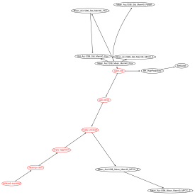
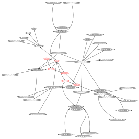
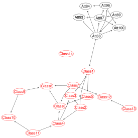
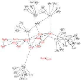
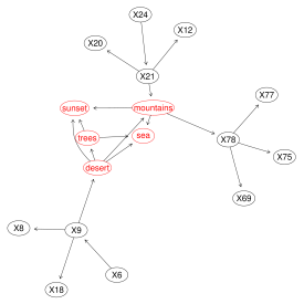
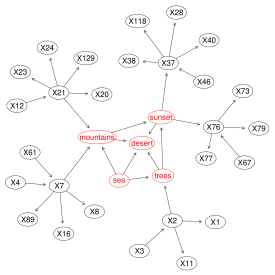
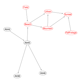
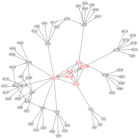
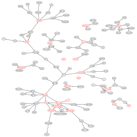
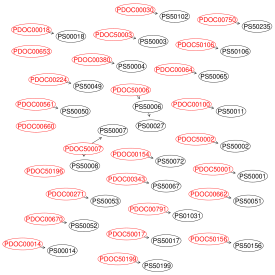
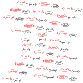
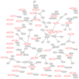
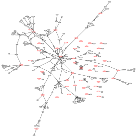
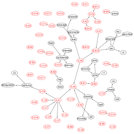
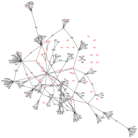
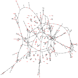
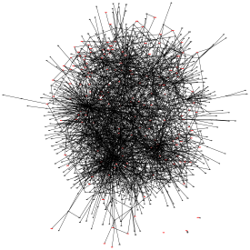
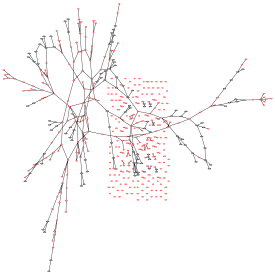
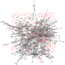
Table 4 reports the outputs of H2PC and MMHC, Table 5 shows the global accuracy of each method on the 10 data sets. Table 6 reports the running time and the average node degree of the labels in the DAGs obtained with both methods. Figures 3 up to 7 display graphically the local DAG structures around the labels, obtained with H2PC and MMHC, for illustration purposes.
Several conclusions may be drawn from these experiments. First, we may observe by inspection of the average degree of the label nodes in Table 6 that several DAGs are densely connected, like scene or bibtex, while others are rather sparse, like genbase, medical, corel5k. The DAGs displayed in Figures 3 up to 7 lend themselves to interpretation. They can be used for encoding as well as portraying the conditional independencies, and the d-sep criterion can be used to read them off the graph. Many label powersets that are reported in Table 4 can be identified by graphical inspection of the DAGs. For instance, the two label powersets in yeast (Figure 3, bottom plot) are clearly noticeable in both DAGs. Clearly, BNs have a number of advantages over alternative methods. They lay bare useful information about the label dependencies which is crucial if one is interested in gaining an understanding of the underlying domain. It is however well beyond the scope of this paper to delve deeper into the DAG interpretation. Overall, it appears that the structures recovered by H2PC are significantly denser, compared to MMHC. On bibtex and enron, the increase of the average label degree is the most spectacular. On bibtex (resp. enron), the average label degree has raised from 2.6 to 6.4 (resp. from 1.2 to 3.3). This result is in nice agreement with the experiments in the previous section, as H2PC was shown to consistently reduce the rate of false negative edges with respect to MMHC (at the cost of a slightly higher false discovery rate).
Second, Table 4 is very instructive as it reveals that on emotions, image, and scene, the MLP approach boils down to the LP scheme. This is easily seen as there is only one minimal label powerset extracted on average. In contrast, on genbase the MLP approach boils down to the simple BR scheme. This is confirmed by inspecting Table 5: the performances of MMHC and H2PC (without feature selection) are equal. An interesting observation upon looking at the distribution of the label powerset size shows that for the remaining data sets, the MLP mostly decomposes the label set in two parts: one on which it performs BR and the other one on which it performs LP. Take for instance enron, it can be seen from Table 4 that there are approximately 23 label singletons and a powerset of 30 labels with H2PC for a total of 53 labels. The gain in performance with MLP over BR, our baseline learner, can be ascribed to the quality of the label powerset decomposition as BR is ignoring label dependencies. As expected, the results using MLP clearly dominate those obtained using BR on all data sets except genbase. The DAGs display the minimum label powersets and their relevant features.
Third, H2PC compares favorably to MMHC. On scene for instance, the accuracy of MLP+MB has raised from 20% (with MMHC) to 56% (with H2PC). On yeast, it has raised from 7% to 23%. Without feature selection, the difference in global accuracy is less pronounced but still in favor of H2PC. A Wilcoxon signed rank paired test reveals statistically significant improvements of H2PC over MMHC in the MLP approach without feature selection (). This trend is more pronounced when the feature selection is used (), using MLP-MB. Note however that the LP decomposition for H2PC and MMHC on yeast and image are strictly identical, hence the same accuracy values in Table 5 in the MLP column.
Fourth, regarding the utility of the feature selection, it is difficult to reach any conclusion. Whether BR or MLP is used, the use of the selected features as inputs to the classification model is not shown greatly beneficial in terms of global accuracy on average. The performance of BR and our MLP with all the features outperforms that with the selected features in 6 data sets but the feature selection leads to actual improvements in 3 data sets. The difference in accuracy with and without the feature selection was not shown to be statistically significant ( with a Wilcoxon signed rank paired test). Surprisingly, the feature selection did exceptionally well on genbase. On this data set, the increase in accuracy is the most impressive: it raised from 7% to 98% which is atypical. The dramatic increase in accuracy on genbase is due solely to the restricted feature set as input to the classification model. This is also observed on medical, to a lesser extent though. Interestingly, on large and densely connected networks (e.g. bibtex, slashdot and corel5K), the feature selection performed very well in terms of global accuracy and significantly reduced the input space which is noticeable. On emotions, yeast, image, scene and genbase, the method reduced the feature set down to nearly 1/100 its original size. The feature selection should be evaluated in view of its effectiveness at balancing the increasing error and the decreasing computational burden by drastically reducing the feature space. We should also keep in mind that the feature relevance cannot be defined independently of the learner and the model-performance metric (e.g., the loss function used). Admittedly, our feature selection based on the Markov boundaries is not necessarily optimal for the base MLC learner used here, namely the Random Forest model.
As far as the overall running time performance is concerned, we see from Table 6 that for both methods, the running time grows somewhat exponentially with the size of the Markov boundary and the number of features, hence the considerable rise in total running time on bibtex. H2PC takes almost 200 times longer on bibtex (1826 variables) and enron (1001 variables) which is quite considerable but still affordable (44 hours of single-CPU time on bibtex and 13 hours on enron). We also observe that the size of the parent set with H2PC is 2.5 (on bibtex) and 3.6 (on enron) times larger than that of MMHC (which may hurt interpretability). In fact, the running time is known to increase exponentially with the parent set size of the true underlying network. This is mainly due the computational overhead of greedy search-and-score procedure with larger parent sets which is the most promising part to optimize in terms of computational gains as we discuss in the Conclusion.
| H2PC | |||||
|---|---|---|---|---|---|
| dataset | # LPs | # labels / LP | # classes / LP | ||
| min/med/max | min/med/max | ||||
| emotions | 6 / 6 / 6 | (6) | 26 / 27 / 27 | (27) | |
| yeast | 2 / 7 / 12 | (14) | 3 / 64 / 135 | (198) | |
| image | 5 / 5 / 5 | (5) | 19 / 20 / 20 | (20) | |
| scene | 6 / 6 / 6 | (6) | 14 / 15 / 15 | (15) | |
| slashdot | 1 / 1 / 14 | (22) | 1 / 2 / 111 | (156) | |
| genbase | 1 / 1 / 2 | (27) | 1 / 2 / 2 | (32) | |
| medical | 1 / 1 / 6 | (45) | 1 / 2 / 10 | (94) | |
| enron | 1 / 1 / 30 | (53) | 1 / 2 / 334 | (753) | |
| bibtex | 1 / 1 / 112 | (159) | 2 / 2 / 1588 | (2856) | |
| corel5k | 1 / 1 / 263 | (374) | 1 / 2 / 2749 | (3175) | |
| MMHC | |||||
| dataset | # LPs | # labels / LP | # classes / LP | ||
| min/med/max | min/med/max | ||||
| emotions | 1 / 6 / 6 | (6) | 2 / 26 / 27 | (27) | |
| yeast | 1 / 7 / 13 | (14) | 2 / 89 / 186 | (198) | |
| image | 5 / 5 / 5 | (5) | 19 / 20 / 20 | (20) | |
| scene | 6 / 6 / 6 | (6) | 14 / 15 / 15 | (15) | |
| slashdot | 1 / 1 / 9 | (22) | 1 / 2 / 46 | (156) | |
| genbase | 1 / 1 / 1 | (27) | 1 / 2 / 2 | (32) | |
| medical | 1 / 1 / 4 | (45) | 1 / 2 / 7 | (94) | |
| enron | 1 / 1 / 12 | (53) | 1 / 2 / 119 | (753) | |
| bibtex | 1 / 1 / 28 | (159) | 2 / 2 / 233 | (2856) | |
| corel5k | 1 / 1 / 177 | (374) | 1 / 2 / 2294 | (3175) | |
| dataset | BR | MLP | BR+MB | MLP+MB | |||
|---|---|---|---|---|---|---|---|
| MMHC | H2PC | MMHC | H2PC | MMHC | H2PC | ||
| emotions | 0.327 | 0.371 | 0.391 | 0.147 | 0.266 | 0.189 | 0.285 |
| yeast | 0.169 | 0.273 | 0.271 | 0.062 | 0.155 | 0.073 | 0.233 |
| image | 0.342 | 0.504 | 0.504 | 0.227 | 0.252 | 0.308 | 0.360 |
| scene | 0.580 | 0.733 | 0.733 | 0.123 | 0.361 | 0.199 | 0.565 |
| slashdot | 0.355 | 0.419 | 0.474 | 0.274 | 0.373 | 0.278 | 0.439 |
| genbase | 0.069 | 0.069 | 0.069 | 0.974 | 0.976 | 0.974 | 0.976 |
| medical | 0.454 | 0.499 | 0.502 | 0.630 | 0.651 | 0.636 | 0.669 |
| enron | 0.134 | 0.165 | 0.180 | 0.024 | 0.079 | 0.079 | 0.157 |
| bibtex | 0.108 | 0.115 | 0.167 | 0.120 | 0.133 | 0.121 | 0.177 |
| corel5k | 0.002 | 0.030 | 0.043 | 0.000 | 0.002 | 0.010 | 0.034 |
| dataset | MMHC | H2PC | ||
|---|---|---|---|---|
| time | label degree | time | label degree | |
| emotions | 1.5 | 16.2 | ||
| yeast | 9.0 | 90.9 | ||
| image | 3.1 | 28.4 | ||
| scene | 9.9 | 662.9 | ||
| slashdot | 44.8 | 822.3 | ||
| genbase | 12.5 | 12.4 | ||
| medical | 43.8 | 334.8 | ||
| enron | 199.8 | 47863.0 | ||
| bibtex | 960.8 | 159469.6 | ||
| corel5k | 169.6 | 2513.0 | ||
6 Discussion & practical applications
Our prime conclusion is that H2PC is a promising approach to constructing BN global or local structures around specific nodes of interest, with potentially thousands of variables. Concentrating on higher recall values while keeping the false positive rate as low as possible pays off in terms of goodness of fit and structure accuracy. Historically, the main practical difficulty in the application of BN structure discovery approaches has been a lack of suitable computing resources and relevant accessible software. The number of variables which can be included in exact BN analysis is still limited. As a guide, this might be less than about 40 variables for exact structural search techniques (Perrier et al., 2008; Kojima et al., 2010). In contrast, constraint-based heuristics like the one presented in this study is capable of processing many thousands of features within hours on a personal computer, while maintaining a very high structural accuracy. H2PC and MMHC could potentially handle up to 10,000 labels in a few days of single-CPU time and far less by parallelizing the skeleton identification algorithm as discussed in (Tsamardinos et al., 2006; Villanueva & Maciel, 2014).
The advantages in terms of structure accuracy and its ability to scale to thousands of variables opens up many avenues of future possible applications of H2PC in various domains as we shall discuss next. For example, BNs have especially proven to be useful abstractions in computational biology (Nagarajan et al., 2013; Scutari & Nagarajan, 2013; Prestat et al., 2013; Aussem et al., 2012, 2010; Peña, 2008; Peña et al., 2005). Identifying the gene network is crucial for understanding the behavior of the cell which, in turn, can lead to better diagnosis and treatment of diseases. This is also of great importance for characterizing the function of genes and the proteins they encode in determining traits, psychology, or development of an organism. Genome sequencing uses high-throughput techniques like DNA microarrays, proteomics, metabolomics and mutation analysis to describe the function and interactions of thousands of genes (Zhang & Zhou., 2006). Learning BN models of gene networks from these huge data is still a difficult task (Badea, 2004; Bernard & Hartemink, 2005; Friedman et al., 1999a; Ott et al., 2004; Pe’er et al., 2001). In these studies, the authors had decide in advance which genes were included in the learning process, in all the cases less than 1000, and which genes were excluded from it (Peña, 2008). H2PC overcome the problem by focusing the search around a targeted gene: the key step is the identification of the vicinity of a node (Peña et al., 2005).
Our second objective in this study was to demonstrate the potential utility of hybrid BN structure discovery to multi-label learning. In multi-label data where many inter-dependencies between the labels may be present, explicitly modeling all relationships between the labels is intuitively far more reasonable (as demonstrated in our experiments). BNs explicitly account for such inter-dependencies and the DAG allows us to identify an optimal set of predictors for every label powerset. The experiments presented here support the conclusion that local structural learning in the form of local neighborhood induction and Markov blanket is a theoretically well-motivated approach that can serve as a powerful learning framework for label dependency analysis geared toward multi-label learning. Multi-label scenarios are found in many application domains, such as multimedia annotation (Snoek et al., 2006; Trohidis et al., 2008), tag recommendation, text categorization (McCallum, 1999; Zhang & Zhou., 2006), protein function classification (Roth & Fischer, 2007), and antiretroviral drug categorization (Borchani et al., 2013).
7 Conclusion & avenues for future research
We first discussed a hybrid algorithm for global or local (around target nodes) BN structure learning called Hybrid HPC (H2PC). Our extensive experiments showed that H2PC outperforms the state-of-the-art MMHC by a significant margin in terms of edge recall without sacrificing the number of extra edges, which is crucial for the soundness of the super-structure used during the second stage of hybrid methods, like the ones proposed in (Perrier et al., 2008; Kojima et al., 2010). The code of H2PC is open-source and publicly available online at https://github.com/madbix/bnlearn-clone-3.4. Second, we discussed an application of H2PC to the multi-label learning problem which is a challenging problem in many real-world application domains. We established theoretical results, under the faithfulness condition, in order to characterize graphically the so-called minimal label powersets that appear as irreducible factors in the joint distribution and their respective Markov boundaries. As far as we know, this is the first investigation of Markov boundary principles to the optimal variable/feature selection problem in multi-label learning. These formal results offer a simple guideline to characterize graphically : i) the minimal label powerset decomposition, (i.e. into minimal subsets such that ), and ii) the minimal subset of features, w.r.t an Information Theory criterion, needed to predict each label powerset, thereby reducing the input space and the computational burden of the multi-label classification. The theoretical analysis laid the foundation for a practical multi-label classification procedure. Another set of experiments were carried out on a broad range of multi-label data sets from different problem domains to demonstrate its effectiveness. H2PC was shown to outperform MMHC by a significant margin in terms of global accuracy.
We suggest several avenues for future research. As far as BN structure learning is concerned, future work will aim at: 1) ascertaining which independence test (e.g. tests targeting specific distributions, employing parametric assumptions etc.) is most suited to the data at hand (Tsamardinos & Borboudakis, 2010; Scutari, 2011); 2) controlling the false discovery rate of the edges in the graph output by H2PC (Peña, 2008) especially when dealing with more nodes than samples, e.g. learning gene networks from gene expression data. In this study, H2PC was run independently on each node without keeping track of the dependencies found previously. This lead to some loss of efficiency due to redundant calculations. The optimization of the H2PC code is currently being undertaken to lower the computational cost while maintaining its performance. These optimizations will include the use of a cache to store the (in)dependencies and the use of a global structure. Other interesting research avenues to explore are extensions and modifications to the greedy search-and-score procedure which is the most promising part to optimize in terms of computational gains. Regarding the multi-label learning problem, experiments with several thousands of labels are currently been conducted and will be reported in due course. We also intend to work on relaxing the faithfulness assumption and derive a practical multi-label classification algorithm based on H2PC that is correct under milder assumptions underlying the joint distribution (e.g. Composition, Intersection). This needs further substantiation through more analysis.
Acknowledgments
The authors thank Marco Scutari for sharing his bnlearn package in R. The research was also supported by grants from the European ENIAC Joint Undertaking (INTEGRATE project) and from the French Rhône-Alpes Complex Systems Institute (IXXI).
Appendix
Lemma 8.
, then .
Proof 1.
To keep the notation uncluttered and for the sake of simplicity, consider a partition of such that , . From the label powerset assumption for and , we have and . From the Decomposition, we have that . Using the Weak union, we obtain that . From these two facts, we can use the Contraction property to show that . Therefore, is a label powerset by definition.
Lemma 9.
Let and denote two distinct labels in and define by and their respective minimal label powerset. Then we have,
Proof 2.
Let us suppose . By the label powerset definition for , we have . As owing to Lemma 8, we have that . , can be decomposed as such that and . Using the Decomposition property, we have that . Using the Weak union property, we have that . As this is true , then , which completes the proof.
Lemma 10.
Consider a minimal label powerset. Then, if satisfies the Composition property, .
Proof 3.
By contradiction, suppose a nonempty exists, such that . From the label powerset assumption of , we have that . From these two facts, we can use the Composition property to show that which contradicts the minimal label powerset assumption of . This concludes the proof.
Theorem 1.
Suppose is faithful to a DAG . Then, and belong to the same minimal label powerset if and only if there exists an undirected path in between nodes and in such that all intermediate nodes are either (i) , or (ii) and has two parents in (i.e. a collider of the form ).
Proof 4.
Suppose such a path exists. By conditioning on all the intermediate colliders in of the form along an undirected path in between nodes and , we ensure that . Due to the faithfulness, this is equivalent to . From Lemma 9, we conclude that and belong to the same minimal label powerset. To show the inverse, note that owing to Lemma 10, we know that there exists no partition of such that . Due to the faithfulness, there exists at least a link between and in the DAG, hence by recursion, there exists a path between and such that all intermediate nodes are either (i) , or (ii) and has two parents in (i.e. a collider of the form ).
Theorem 1.
Suppose is faithful to a DAG . Let be a label powerset. Then, its Markov boundary in is also its Markov boundary in , and is given in by .
Proof 5.
First, we prove that is a Markov boundary of in . Define the Markov boundary of in , and . From Theorem 5, is given in by . We may now prove that is a Markov boundary of in . We show first that the statement holds for and then conclude that it holds for all by induction. Let denote , and define and . From the Markov blanket assumption for we have . Using the Weak Union property, we obtain that . Similarly we can derive . Combining these two statements yields due to the Intersection property. Let the last expression can be formulated as which is the definition of a Markov blanket of in . We shall now prove that is minimal. Let us suppose that it is not the case, i.e., such that . Define and , we may apply the Weak Union property to get which can be rewritten more compactly as . From the Markov blanket assumption, we have . We may now apply the Intersection property on these two statements to obtain . Similarly, we can derive . From the Markov boundary assumption of and , we have necessarily and , which in turn yields . To conclude for any , it suffices to set and to conclude by induction.
Second, we prove that is a Markov blanket of in . Define . From the label powerset definition, we have . Using the Weak Union property, we obtain which can be reformulated as . Now, the Markov blanket assumption for in yields which can be rewritten as . From the Intersection property, we get . From the Markov boundary assumption of in , we know that there exists no proper subset of which satisfies this statement, and therefore . From the Markov blanket assumption of in , we have . Using the Decomposition property, we obtain which, together with the assumption , is the definition of a Markov blanket of in .
Finally, we prove that is a Markov boundary of in . Let us suppose that it is not the case, i.e., such that . From the label powerset assumption of , we have which can be rewritten as . Due to the Contraction property, combining these two statements yields . From the Markov boundary assumption of in , we have necessarily , which suffices to prove that is a Markov boundary of in .

References
- Agresti (2002) Agresti, A. (2002). Categorical Data Analysis. Wiley, 2nd edition.
- Aliferis et al. (2010) Aliferis, C. F., Statnikov, A. R., Tsamardinos, I., Mani, S., & Koutsoukos, X. D. (2010). Local causal and markov blanket induction for causal discovery and feature selection for classification part i: Algorithms and empirical evaluation. Journal of Machine Learning Research, JMLR, 11, 171–234.
- Alvares-Cherman et al. (2011) Alvares-Cherman, E., Metz, J., & Monard, M. (2011). Incorporating label dependency into the binary relevance framework for multi-label classification. Expert Systems With Applications, ESWA, 39, 1647–1655.
- Armen & Tsamardinos (2011) Armen, A. P., & Tsamardinos, I. (2011). A unified approach to estimation and control of the false discovery rate in bayesian network skeleton identification. In European Symposium on Artificial Neural Networks, ESANN.
- Aussem et al. (2012) Aussem, A., Rodrigues de Morais, S., & Corbex, M. (2012). Analysis of nasopharyngeal carcinoma risk factors with bayesian networks. Artificial Intelligence in Medicine, 54.
- Aussem et al. (2010) Aussem, A., Tchernof, A., Rodrigues de Morais, S., & Rome, S. (2010). Analysis of lifestyle and metabolic predictors of visceral obesity with bayesian networks. BMC Bioinformatics, 11, 487.
- Badea (2004) Badea, A. (2004). Determining the direction of causal influence in large probabilistic networks: A constraint-based approach. In Proceedings of the Sixteenth European Conference on Artificial Intelligence (pp. 263–267).
- Bernard & Hartemink (2005) Bernard, A., & Hartemink, A. (2005). Informative structure priors: Joint learning of dynamic regulatory networks from multiple types of data. In Proceedings of the Pacific Symposium on Biocomputing (pp. 459–470).
- Blockeel et al. (1998) Blockeel, H., Raedt, L. D., & Ramon, J. (1998). Top-down induction of clustering trees. In J. W. Shavlik (Ed.), International Conference on Machine Learning, ICML (pp. 55–63). Morgan Kaufmann.
- Borchani et al. (2013) Borchani, H., Bielza, C., Toro, C., & Larrañaga, P. (2013). Predicting human immunodeficiency virus inhibitors using multi-dimensional bayesian network classifiers. Artificial Intelligence in Medicine, 57, 219–229.
- Breiman (2001) Breiman, L. (2001). Random forests. Machine Learning, 45, 5–32.
- Brown & Tsamardinos (2008) Brown, L. E., & Tsamardinos, I. (2008). A strategy for making predictions under manipulation. Journal of Machine Learning Research, JMLR, 3, 35–52.
- Buntine (1991) Buntine, W. (1991). Theory refinement on Bayesian networks. In B. D’Ambrosio, P. Smets, & P. Bonissone (Eds.), Uncertainty in Artificial Intelligence, UAI (pp. 52–60). San Mateo, CA, USA: Morgan Kaufmann Publishers.
- Cawley (2008) Cawley, G. (2008). Causal and non-causal feature selection for ridge regression. JMLR: Workshop and Conference Proceedings, 3, 107–128.
- Cheng et al. (2002) Cheng, J., Greiner, R., Kelly, J., Bell, D. A., & Liu, W. (2002). Learning Bayesian networks from data: An information-theory based approach. Artificial Intelligence, 137, 43–90.
- Chickering et al. (2004) Chickering, D., Heckerman, D., & Meek, C. (2004). Large-sample learning of Bayesian networks is NP-hard. Journal of Machine Learning Research, JMLR, 5, 1287–1330.
- Chickering (2002) Chickering, D. M. (2002). Optimal structure identification with greedy search. Journal of Machine Learning Research, JMLR, 3, 507–554.
- Cussens & Bartlett (2013) Cussens, J., & Bartlett, M. (2013). Advances in Bayesian Network Learning using Integer Programming. In Uncertainty in Artificial Intelligence (pp. 182–191).
- Dembczyński et al. (2012) Dembczyński, K., Waegeman, W., Cheng, W., & Hüllermeier, E. (2012). On label dependence and loss minimization in multi-label classification. Machine Learning, 88, 5–45.
- Ellis & Wong (2008) Ellis, B., & Wong, W. H. (2008). Learning causal bayesian network structures from experimental data. Journal of the American Statistical Association, 103, 778–789.
- Friedman et al. (1999a) Friedman, N., Nachman, I., , & Pe’er, D. (1999a). Learning bayesian network structure from massive datasets: The “sparse candidate” algorithm. In Proceedings of the Fifteenth Conference on Uncertainty in Artificial Intelligence (pp. 206–215).
- Friedman et al. (1999b) Friedman, N., Nachman, I., & Pe’er, D. (1999b). Learning bayesian network structure from massive datasets: the ”sparse candidate” algorithm. In K. B. Laskey, & H. Prade (Eds.), Uncertainty in Artificial Intelligence, UAI (pp. 21–30). Morgan Kaufmann Publishers.
- Gasse et al. (2012) Gasse, M., Aussem, A., & Elghazel, H. (2012). Comparison of hybrid algorithms for bayesian network structure learning. In European Conference on Machine Learning and Principles and Practice of Knowledge Discovery in Databases, ECML-PKDD (pp. 58–73). Springer volume 7523 of Lecture Notes in Computer Science.
- Gu et al. (2011) Gu, Q., Li, Z., & Han, J. (2011). Correlated multi-label feature selection. In C. Macdonald, I. Ounis, & I. Ruthven (Eds.), CIKM (pp. 1087–1096). ACM.
- Guo & Gu (2011) Guo, Y., & Gu, S. (2011). Multi-label classification using conditional dependency networks. In International Joint Conference on Artificial Intelligence, IJCAI (pp. 1300–1305). AAAI Press.
- Heckerman et al. (1995) Heckerman, D., Geiger, D., & Chickering, D. (1995). Learning bayesian networks: The combination of knowledge and statistical data. Machine Learning, 20, 197–243.
- Kocev et al. (2007) Kocev, D., Vens, C., Struyf, J., & Džeroski, S. (2007). Ensembles of multi-objective decision trees. In J. N. Kok (Ed.), European Conference on Machine Learning, ECML (pp. 624–631). Springer volume 4701 of Lecture Notes in Artificial Intelligence.
- Koivisto & Sood (2004) Koivisto, M., & Sood, K. (2004). Exact bayesian structure discovery in bayesian networks. Journal of Machine Learning Research, JMLR, 5, 549–573.
- Kojima et al. (2010) Kojima, K., Perrier, E., Imoto, S., & Miyano, S. (2010). Optimal search on clustered structural constraint for learning bayesian network structure. Journal of Machine Learning Research, JMLR, 11, 285–310.
- Koller & Friedman (2009) Koller, D., & Friedman, N. (2009). Probabilistic Graphical Models: Principles and Techniques. MIT Press.
- Koller & Sahami (1996) Koller, D., & Sahami, M. (1996). Toward optimal feature selection. In International Conference on Machine Learning, ICML (pp. 284–292).
- Liaw & Wiener (2002) Liaw, A., & Wiener, M. (2002). Classification and regression by randomforest. R News, 2, 18–22.
- Luaces et al. (2012) Luaces, O., Díez, J., Barranquero, J., del Coz, J. J., & Bahamonde, A. (2012). Binary relevance efficacy for multilabel classification. Progress in AI, 1, 303–313.
- Madjarov et al. (2012) Madjarov, G., Kocev, D., Gjorgjevikj, D., & Džeroski, S. (2012). An extensive experimental comparison of methods for multi-label learning. Pattern Recognition, 45, 3084–3104.
- Maron & Ratan (1998) Maron, O., & Ratan, A. L. (1998). Multiple-Instance Learning for Natural Scene Classification. In International Conference on Machine Learning, ICML (pp. 341–349). Citeseer volume 7.
- McCallum (1999) McCallum, A. (1999). Multi-label text classification with a mixture model trained by em. In AAAI Workshop on Text Learning.
- Moore & Wong (2003) Moore, A., & Wong, W. (2003). Optimal reinsertion: A new search operator for accelerated and more accurate Bayesian network structure learning. In T. Fawcett, & N. Mishra (Eds.), International Conference on Machine Learning, ICML.
- Nagarajan et al. (2013) Nagarajan, R., Scutari, M., & Lèbre, S. (2013). Bayesian Networks in R: with Applications in Systems Biology (Use R!). Springer.
- Neapolitan (2004) Neapolitan, R. E. (2004). Learning Bayesian Networks. Upper Saddle River, NJ: Pearson Prentice Hall.
- Ott et al. (2004) Ott, S., Imoto, S., & Miyano, S. (2004). Finding optimal models for small gene networks. In Proceedings of the Pacific Symposium on Biocomputing (pp. 557–567).
- Peña et al. (2007) Peña, J., Nilsson, R., Björkegren, J., & Tegnér, J. (2007). Towards scalable and data efficient learning of Markov boundaries. International Journal of Approximate Reasoning, 45, 211–232.
- Peña et al. (2005) Peña, J. M., Björkegren, J., & Tegnér, J. (2005). Growing Bayesian network models of gene networks from seed genes. Bioinformatics, 40, 224–229.
- Pearl (1988) Pearl, J. (1988). Probabilistic Reasoning in Intelligent Systems: Networks of Plausible Inference.. San Francisco, CA, USA: Morgan Kaufmann.
- Peña (2008) Peña, J. M. (2008). Learning gaussian graphical models of gene networks with false discovery rate control. In European Conference on Evolutionary Computation, Machine Learning and Data Mining in Bioinformatics 6 (pp. 165–176).
- Peña (2012) Peña, J. M. (2012). Finding consensus bayesian network structures. Journal of Artificial Intelligence Research, 42, 661–687.
- Perrier et al. (2008) Perrier, E., Imoto, S., & Miyano, S. (2008). Finding optimal bayesian network given a super-structure. Journal of Machine Learning Research, JMLR, 9, 2251–2286.
- Pe’er et al. (2001) Pe’er, D., Regev, A., Elidan, G., & Friedman, N. (2001). Inferring subnetworks from perturbed expression profiles. Bioinformatics, 17, 215–224.
- Prestat et al. (2013) Prestat, E., Rodrigues de Morais, S., Vendrell, J., Thollet, A., Gautier, C., Cohen, P., & Aussem, A. (2013). Learning the local Bayesian network structure around the ZNF217 oncogene in breast tumours. Computers in Biology and Medicine, 4, 334–341.
- R Core Team (2013) R Core Team (2013). R: A Language and Environment for Statistical Computing. R Foundation for Statistical Computing Vienna, Austria. URL: http://www.R-project.org.
- Read et al. (2009) Read, J., Pfahringer, B., Holmes, G., & Frank, E. (2009). Classifier chains for multi-label classification. In European Conference on Machine Learning and Principles and Practice of Knowledge Discovery in Databases, ECML-PKDD (pp. 254–269). Springer volume 5782 of Lecture Notes in Computer Science.
- Rodrigues de Morais & Aussem (2010a) Rodrigues de Morais, S., & Aussem, A. (2010a). An efficient learning algorithm for local bayesian network structure discovery. In European Conference on Machine Learning and Principles and Practice of Knowledge Discovery in Databases, ECML-PKDD (pp. 164–169).
- Rodrigues de Morais & Aussem (2010b) Rodrigues de Morais, S., & Aussem, A. (2010b). A novel Markov boundary based feature subset selection algorithm. Neurocomputing, 73, 578–584.
- Roth & Fischer (2007) Roth, V., & Fischer, B. (2007). Improved functional prediction of proteins by learning kernel combinations in multilabel settings. BMC Bioinformatics, 8, S12+.
- Schwarz (1978) Schwarz, G. E. (1978). Estimating the dimension of a model. Journal of Biomedical Informatics, 6, 461–464.
- Scutari (2010) Scutari, M. (2010). Learning bayesian networks with the bnlearn R package. Journal of Statistical Software, 35, 1–22.
- Scutari (2011) Scutari, M. (2011). Measures of Variability for Graphical Models. Ph.D. thesis School in Statistical Sciences, University of Padova.
- Scutari & Brogini (2012) Scutari, M., & Brogini, A. (2012). Bayesian network structure learning with permutation tests. Communications in Statistics – Theory and Methods, 41, 3233–3243.
- Scutari & Nagarajan (2013) Scutari, M., & Nagarajan, R. (2013). Identifying significant edges in graphical models of molecular networks. Artificial Intelligence in Medicine, 57, 207–217.
- Silander & Myllymäki (2006) Silander, T., & Myllymäki, P. (2006). A Simple Approach for Finding the Globally Optimal Bayesian Network Structure. In Uncertainty in Artificial Intelligence, UAI (pp. 445–452).
- Snoek et al. (2006) Snoek, C., Worring, M., Gemert, J. V., Geusebroek, J., & Smeulders, A. (2006). The challenge problem for automated detection of 101 semantic concepts in multimedia. In ACM International Conference on Multimedia (pp. 421–430). ACM Press.
- Spirtes et al. (2000) Spirtes, P., Glymour, C., & Scheines, R. (2000). Causation, Prediction, and Search. (2nd ed.). The MIT Press.
- Spolaôr et al. (2013) Spolaôr, N., Cherman, E. A., Monard, M. C., & Lee, H. D. (2013). A comparison of multi-label feature selection methods using the problem transformation approach. Electronic Notes in Theoretical Computer Science, 292, 135–151.
- Studený & Haws (2014) Studený, M., & Haws, D. (2014). Learning Bayesian network structure: Towards the essential graph by integer linear programming tools. International Journal of Approximate Reasoning, 55, 1043–1071.
- Trohidis et al. (2008) Trohidis, K., Tsoumakas, G., Kalliris, G., & Vlahavas, I. (2008). Multi-label classification of music into emotions. In ISMIR (pp. 325–330).
- Tsamardinos et al. (2003) Tsamardinos, I., Aliferis, C., & Statnikov, A. (2003). Algorithms for large scale Markov blanket discovery. In Florida Artificial Intelligence Research Society Conference FLAIRS’03 (pp. 376–381).
- Tsamardinos & Borboudakis (2010) Tsamardinos, I., & Borboudakis, G. (2010). Permutation testing improves bayesian network learning. In European Conference on Machine Learning and Knowledge Discovery in Databases, ECML-PKDD (pp. 322–337).
- Tsamardinos et al. (2006) Tsamardinos, I., Brown, L., & Aliferis, C. (2006). The Max-Min Hill-Climbing Bayesian Network Structure Learning Algorithm. Machine Learning, 65, 31–78.
- Tsamardinos & Brown (2008) Tsamardinos, I., & Brown, L. E. (2008). Bounding the false discovery rate in local Bayesian network learning. In AAAI Conference on Artificial Intelligence (pp. 1100–1105).
- Tsoumakas et al. (2010a) Tsoumakas, G., Katakis, I., & Vlahavas, I. (2010a). Mining Multi-label Data. Transformation, 135, 1–20.
- Tsoumakas et al. (2010b) Tsoumakas, G., Katakis, I., & Vlahavas, I. (2010b). Random k-labelsets for Multi-Label Classification. IEEE Transactions on Knowledge and Data Engineering, TKDE, 23, 1–12.
- Tsoumakas & Vlahavas (2007) Tsoumakas, G., & Vlahavas, I. (2007). Random k-labelsets: An ensemble method for multilabel classification. Proceedings of the 18th European Conference on Machine Learning, 4701, 406–417.
- Villanueva & Maciel (2012) Villanueva, E., & Maciel, C. (2012). Optimized algorithm for learning bayesian network superstructures. In International Conference on Pattern Recognition Applications and Methods, ICPRAM.
- Villanueva & Maciel (2014) Villanueva, E., & Maciel, C. D. (2014). Efficient methods for learning bayesian network super-structures. Neurocomputing, (pp. 3–12).
- Zhang & Zhang (2010) Zhang, M. L., & Zhang, K. (2010). Multi-label learning by exploiting label dependency. In European Conference on Machine Learning and Principles and Practice of Knowledge Discovery in Databases, ECML PKDD (p. 999). ACM Press volume 16 of Knowledge Discovery in Databases, KDD.
- Zhang & Zhou. (2006) Zhang, M.-L., & Zhou., Z.-H. (2006). Multilabel neural networks with applications to functional genomics and text categorization. IEEE Transactions on Knowledge and Data Engineering, 18, 1338 – 1351.