A New Perspective on Clustered Planarity
as a
Combinatorial Embedding Problem††thanks: Partly done within GRADR –
EUROGIGA project no. 10-EuroGIGA-OP-003. Supported by a
fellowship within the Postdoc-Program of the German Academic
Exchange Service (DAAD).
{blaesius,rutter}@kit.edu)
Abstract
The clustered planarity problem (c-planarity) asks whether a hierarchically clustered graph admits a planar drawing such that the clusters can be nicely represented by regions. We introduce the cd-tree data structure and give a new characterization of c-planarity. It leads to efficient algorithms for c-planarity testing in the following cases. (i) Every cluster and every co-cluster (complement of a cluster) has at most two connected components. (ii) Every cluster has at most five outgoing edges.
Moreover, the cd-tree reveals interesting connections between c-planarity and planarity with constraints on the order of edges around vertices. On one hand, this gives rise to a bunch of new open problems related to c-planarity, on the other hand it provides a new perspective on previous results.
keywords:
graph drawing, clustered planarity, constrained planar embedding, characterization, algorithms1 Introduction
When visualizing graphs whose nodes are structured in a hierarchy, one usually has two objectives. First, the graph should be drawn nicely. Second, the hierarchical structure should be expressed by the drawing. Regarding the first objective, we require drawings without edge crossings, i.e., planar drawings (the number of crossings in a drawing of a graph is a major aesthetic criterion). A natural way to represent a cluster is a simple region containing exactly the vertices in the cluster. To express the hierarchical structure, the boundaries of two regions must not cross and edges of the graph can cross region boundaries at most once, namely if only one of its endpoints lies inside the cluster. Such a drawing is called c-planar; see Section 2 for a formal definition. Testing a clustered graph for c-planarity (i.e., testing whether it admits a c-planar drawing) is a fundamental open problem in the field of Graph Drawing.
C-planarity was first considered by Lengauer [23] but in a completely different context. He gave an efficient algorithm for the case that every cluster is connected. Feng et al. [15], who coined the name c-planarity, rediscovered the problem and gave a similar algorithm. Cornelsen and Wagner [8] showed that c-planarity is equivalent to planarity when every cluster and every co-cluster is connected.
Relaxing the condition that every cluster must be connected, makes testing c-planarity surprisingly difficult. Efficient algorithms are known only for very restricted cases and many of these algorithms are very involved. One example is the efficient algorithm by Jelínek et al. [20, 19] for the case that every cluster consists of at most two connected components while the planar embedding of the underlying graph is fixed. Another efficient algorithm by Jelínek et al. [21] solves the case that every cluster has at most four outgoing edges.
A popular restriction is to require a flat hierarchy, i.e., every pair of clusters has empty intersection. For example, Di Battista and Frati [14] solve the case where the clustering is flat, the graph has a fixed planar embedding and the size of the faces is bounded by five. Section 4.1.1 and Section 4.2.1 contain additional related work viewed from the new perspective.
1.1 Contribution & Outline
We first present the cd-tree data structure (Section 3), which is similar to a data structure used by Lengauer [23]. We use the cd-tree to characterize c-planarity in terms of a combinatorial embedding problem. We believe that our definition of the cd-tree together with this characterization provides a very useful perspective on the c-planarity problem and significantly simplifies some previous results.
In Section 4 we define different constrained-planarity problems. We use the cd-tree to show in Section 4.1 that these problems are equivalent to different versions of the c-planarity problem on flat-clustered graphs. We also discuss which cases of the constrained embedding problems are solved by previous results on c-planarity of flat-clustered graphs. Based on these insights, we derive a generic algorithm for testing c-planarity with different restrictions in Section 4.2 and discuss previous work in this context.
In Section 5, we show how the cd-tree characterization together with results on the problem Simultaneous PQ-Ordering [4] lead to efficient algorithms for the cases that (i) every cluster and every co-cluster consists of at most two connected components; or (ii) every cluster has at most five outgoing edges. The latter extends the result by Jelínek et al. [21], where every cluster has at most four outgoing edges.
2 Preliminaries
We denote graphs by with vertex set and edge set . We implicitly assume graphs to be simple, i.e., they do not have multiple edges or loops. Sometimes we allow multiple edges (we never allow loops). We indicate this with the prefix multi-, e.g., a multi-cycle is a graph obtained from a cycle by multiplying edges.
A (multi-)graph is planar if it admits a planar drawing (no edge crossings). The edge-ordering of a vertex is the clockwise cyclic order of its incident edges in a planar drawing of . A (planar) embedding of consists of an edge-ordering for every vertex such that admits a planar drawing with these edge-orderings.
A PQ-tree [5] is a tree (in our case unrooted) with leaves such that every inner node is either a P-node or a Q-node. When embedding , one can choose the (cyclic) edge-orderings of P-nodes arbitrarily, whereas the edge-orderings of Q-nodes are fixed up to reversal. Every such embedding of defines a cyclic order on the leaves . The PQ-tree represents the orders one can obtain in this way. A set of orders is PQ-representable if it can be represented by a PQ-tree. It is not hard to see that the valid edge-orderings of non-cutvertices in planar graphs are PQ-representable (e.g., [4]). Conversely, adding wheels around the Q-nodes of a PQ-tree and connecting all leaves with a vertex yields a planar graph where the edge-orderings of in embeddings of are represented by (e.g., [23]).
2.1 C-Planarity on the Plane and on the Sphere
A clustered graph is a graph together with a rooted tree whose leaves are the vertices of . Let be a node of . The tree is the subtree of consisting of all successors of together with the root . The graph induced by the leaves of is a cluster in . We identify this cluster with the node . We call a cluster proper if it is neither the whole graph (root cluster) nor a single vertex (leaf cluster).
A c-planar drawing of is a planar drawing of in the plane together with a simple (= simply-connected) region for every cluster satisfying the following properties. (i) Every region contains exactly the vertices of the cluster . (ii) Two regions have non-empty intersection only if one contains the other. (iii) Edges cross the boundary of a region at most once. A clustered graph is c-planar if and only if it admits a c-planar drawing.
The above definition of c-planarity relies on embeddings in the plane using terms like “outside” and “inside”. Instead, one can consider drawings on the sphere by considering the tree to be unrooted instead of rooted, using cuts instead of clusters, and simple closed curves instead of simple regions. Let be an edge in . Removing splits in two connected components. As the leaves of are the vertices of , this induces a corresponding cut with on . For a c-planar drawing of on the sphere, we require a planar drawing of together with a simple closed curve for every cut with the following properties. (i) The curve separates from . (ii) No two curves intersect. (iii) Edges of cross at most once.
Note that using clusters instead of cuts corresponds to orienting the cuts, using one side as the cluster and the other side as the cluster’s complement (the co-cluster). This notion of c-planarity on the sphere is equivalent to the one on the plane; one simply has to choose an appropriate point on the sphere to lie in the outer face. The unrooted view has the advantage that it is more symmetric (i.e., there is no difference between clusters and co-clusters), which is sometimes desirable. We use the rooted and unrooted view interchangeably.
3 The CD-Tree
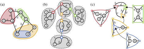
Let be a clustered graph. We introduce the cd-tree (cut- or cluster-decomposition-tree) by enhancing each node of with a multi-graph that represents the decomposition of along its cuts corresponding to edges in ; see Fig. 1a and b for an example. We note that Lengauer [23] uses a similar structure. Our notation is inspired by SPQR-trees [13].
Let be a node of with neighbors and incident edges (for ). Removing separates into subtrees . Let be the vertices of represented by leaves in these subtrees. The skeleton of is the multi-graph obtained from by contracting each subset into a single vertex (the resulting graph has multiple edges but we remove loops). These vertices are called virtual vertices. Note that skeletons of inner nodes of contain only virtual vertices, while skeletons of leaves consist of one virtual and one non-virtual vertex. The node is the neighbor of corresponding to and the virtual vertex in corresponding to is the twin of , denoted by . Note that .
The edges incident to are exactly the edges of crossing the cut corresponding to the tree edge . Thus, the same edges of are incident to and . This gives a bound on the total size of the cd-tree’s skeletons (which we shortly call the size of the cd-tree). The total number of edges in skeletons of is twice the total size of all cuts represented by . As edges might cross a linear number of cuts (but obviously not more), the cd-tree has at most quadratic size in the number of vertices of , i.e., .
Assume the cd-tree is rooted. Recall that in this case every node represents a cluster of . In analogy to the notion for SPQR-trees, we define the pertinent graph of the node to be the cluster represented by . Note that one could also define the pertinent graph recursively, by removing the virtual vertex corresponding to the parent of (the parent vertex) from and replacing each remaining virtual vertex by the pertinent graph of the corresponding child of sy. Clearly, the pertinent graph of a leaf of is a single vertex and the pertinent graph of the root is the whole graph . A similar concept, also defined for unrooted cd-trees, is the expansion graph. The expansion graph of a virtual vertex in is the pertinent graph of its corresponding neighbor of , when rooting at . One can think of the expansion graph as the subgraph of represented by in . As mentioned before, we use the rooted and unrooted points of view interchangeably.
The leaves of a cd-tree represent singleton clusters that exist only due to technical reasons. It is often more convenient to consider cd-trees with all leaves removed as follows. Let be a node with virtual vertex in that corresponds to a leaf. The leaf contains and a non-virtual vertex in its skeleton (with an edge between and for each edge incident to in ). We replace in with the non-virtual vertex and remove the leaf containing . Clearly, this preserves all clusters except for the singleton cluster. Moreover, the graph represented by the cd-tree remains unchanged as we replaced the virtual vertex by its expansion graph . In the following we always assume the leaves of cd-trees to be removed.
3.1 The CD-Tree Characterization
We show that c-planarity testing can be expressed in terms of edge-orderings in embeddings of the skeletons of .
Theorem 1.
A clustered graph is c-planar if and only if the skeletons of all nodes in its cd-tree can be embedded such that every virtual vertex and its twin have the same edge-ordering.
Proof.
Assume admits a c-planar drawing on the sphere. Let be a node of with incident edges connecting to its neighbors , respectively. Let further be the virtual vertex in corresponding to and let be the nodes in the expansion graph . For every cut (with ), contains a simple closed curve representing it. Since the are disjoint, we can choose a point on the sphere to be the outside such that lies inside for . Since is a c-planar drawing, the do not intersect and only the edges of crossing the cut cross exactly once. Thus, one can contract the inside of to a single point while preserving the embedding of . Doing this for each of the curves yields the skeleton together with a planar embedding. Moreover, the edge-ordering of the vertex is the same as the order in which the edges cross the curve , when traversing in clockwise direction. Applying the same construction for the neighbour corresponding to yields a planar embedding of in which the edge-ordering of is the same as the order in which these edges cross the curve , when traversing in counter-clockwise direction. Thus, in the resulting embeddings of the skeletons, the edge-ordering of a virtual vertex and its twin is the same up to reversal. To make them the same one can choose a 2-coloring of and mirror the embeddings of all skeletons of nodes in one color class.
Conversely, assume that all skeletons are embedded such that every virtual vertex and its twin have the same edge-ordering. Let be a node of . Consider a virtual vertex of with edge-ordering . We replace by a cycle and attach the edge to the vertex ; see Fig. 1c. Recall that has in the same incident edges and they also appear in this order around . We also replace by a cycle of length . We say that this cycle is the twin of and denote it by where denotes the new vertex incident to the edge . As the interiors of and are empty, we can glue the skeletons and together by identifying the vertices of with the corresponding vertices in (one of the mbeddings has to be flipped). Applying this replacement for every virtual vertex and gluing it with its twin leads to an embedded planar graph with the following properties. First, contains a subdivision of . Second, for every cut corresponding to an edge in , contains the cycle with exactly one subdivision vertex of an edge of if the cut corresponding to separates the endpoints of . Third, no two of these cycles share a vertex. The planar drawing of gives a planar drawing of . Moreover, the drawings of the cycles can be used as curves representing the cuts, yielding a c-planar drawing of . ∎
3.2 Cutvertices in Skeletons
We show that cutvertices in skeletons correspond to different connected components in a cluster or in a co-cluster. More precisely, a cutvertex directly implies disconnectivity, while the opposite is not true. Consider the example in Fig. 1. The cutvertex in the skeleton containing the vertices and corresponds to the two connected components in the blue cluster (containing and ). However, the two connected components in the orange cluster (containing –) do not yield a new cutvertex in the skeleton containing the vertex . The following lemma in particular shows that requiring every cluster to be connected implies that the parent vertices of skeletons cannot be cutvertices.
Lemma 1.
Let be a virtual vertex that is a cutvertex in its skeleton. The expansion graphs of virtual vertices in different blocks incident to belong to different connected components in .
Proof.
Let be the node whose skeleton contains . Recall that one can obtain the graph by removing from and replacing all other virtual vertices of with their expansion graphs. Clearly, this yields (at least) one different connected component for each of the blocks incident to . ∎
While the converse of Lemma 1 is generally not true, it holds if the condition is satisfied for all parent vertices in all skeletons simultaneously.
Lemma 2.
Every cluster in a clustered graph is connected if and only if in every node of the rooted cd-tree the parent vertex is not a cutvertex in .
Proof.
By Lemma 1, the existence of a cutvertex implies a disconnected cluster. Conversely, let be disconnected and assume without loss of generality that is connected for every child of in the cd-tree. One obtains without the parent vertex by contracting in the child clusters to virtual vertices . As the contracted graphs are connected while the initial graph is not, the resulting graph must be disconnected. Thus, is a cutvertex in . ∎
4 Clustered and Constrained Planarity
We first describe several constraints on planar embeddings, each restricting the edge-orderings of vertices. We then show the relation to c-planarity.
Consider a finite set (e.g., edges incident to a vertex). Denote the set of all cyclic orders of by . An order-constraint on is simply a subset of (only the orders in the subset are allowed). A family of order-constraints for the set is a set of different order constraints, i.e., a subset of the power set of . We say that a family of order-constraints has a compact representation, if one can specify every order-constraint in this family with polynomial space (in ). In the following we describe families of order-constraints with compact representations.
A partition-constraint is given by partitioning into subsets . It requires that no two partitions alternate, i.e., elements and must not appear in the order . A PQ-constraint requires that the order of elements in is represented by a given PQ-tree with leaves . A full-constraint contains only one order, i.e., the order of is completely fixed.
A partitioned full-constraint restricts the orders of elements in according to a partition constraint (partitions must not alternate) and additionally completely fixes the order within each partition. Similarly, partitioned PQ-constraints require the elements in each partition to be ordered according to a PQ-constraint. Clearly, this notion of partitioned order-constraints generalizes to arbitrary order-constraints.
Consider a planar graph . By constraining a vertex of , we mean that there is an order-constraint on the edges incident to . We then only allow planar embeddings of where the edge-ordering of is allowed by the order-constraint. By constraining , we mean that several (or all) vertices of are constrained.
4.1 Flat-Clustered Graph
Consider a flat-clustered graph, i.e., a clustered graph where the cd-tree is a star. We choose the center of the star to be the root. Let be the virtual vertices in corresponding to the children of . Note that contains exactly one virtual vertex, namely . The possible ways to embed restrict the possible edge-orderings of and thus, by the characterization in Theorem 1, the edge-orderings of in . Hence, the graph essentially yields an order constraint for in . We consider c-planarity with differently restricted instances, leading to different families of order-constraints. To show that testing c-planarity is equivalent to testing whether is planar with respect to order-constraints of a specific family, we have to show two directions. First, the embeddings of only yield order-constraints of the given family. Second, we can get every possible order-constraint of the given family by choosing an appropriate graph for .
Theorem 2.
Testing c-planarity of flat-clustered graphs (i) where each proper cluster consists of isolated vertices; (ii) where each cluster is connected; (iii) with fixed planar embedding; (iv) without restriction is linear-time equivalent to testing planarity of a multi-graph with (i) partition-constraints; (ii) PQ-constraints; (iii) partitioned full-constraints; (iv) partitioned PQ-constraints, respectively.
Proof.
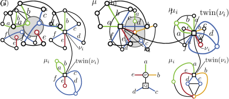
We start with case (i); see Fig. 2a. Consider a flat-clustered graph and let be one of the leaves of the cd-tree. As is a proper cluster, it consists of isolated vertices. Thus, is a set of vertices , each connected (with multiple edges) to the virtual vertex . The vertices partition the edges incident to into subsets. Clearly, in every planar embedding of no two partitions alternate. Moreover, every edge-ordering of in which no two partitions alternate gives a planar embedding of . Thus, the edges incident to in are constrained by a partition-constraint, where the partitions are determined by the incidence of the edges to the vertices . One can easily construct the resulting instance of planarity with partition-constraints problem in linear time in the size of the cd-tree. Note that the cd-tree has linear size in for flat-clustered graphs.
Conversely, given a planar graph with partition-constraints, we set . For every vertex of we have a virtual vertex in with corresponding child . We can simulate every partitioning of the edges incident to by connecting edges incident to (in ) with vertices such that two edges are connected to the same vertex if and only if they belong to the same partition. Clearly, this construction runs in linear time.
Case (ii) is illustrated in Fig. 2b. By Lemma 2 the condition of connected clusters is equivalent to requiring that the virtual vertex in the skeleton of any leaf of the cd-tree is not a cutvertex. The statement of the theorem follows from the fact that the possible edge-orderings of non-cutvertices is PQ-representable and that any PQ-tree can be achieved by choosing an appropriate planar graph in which is not a cutvertex (see Section 2).
In case (iii) the embedding of is fixed. As in case (i), the blocks incident to in partition the edges incident to in such that two partitions must not alternate. Moreover, the fixed embedding of fixes the edge-ordering of non-virtual vertices and thus it fixes the embeddings of the blocks in . Hence, we get partitioned full-constraints for . Conversely, we can construct an arbitrary partitioned full-constraint as in case (i).
For case (iv) the arguments from case (iii) show that we again get partitioned order-constraints, while the arguments from case (ii) show that these order-constraints (for the blocks) are PQ-constraints. ∎
4.1.1 Related Work
Biedl [1] proposes different drawing-models for graphs whose vertices are partitioned into two subsets. The model matching the requirements of c-planar drawings is called HH-drawings. Biedl et al. [2] show that one can test for the existence of HH-drawings in linear time. Hong and Nagamochi [18] rediscovered this result in the context of 2-page book embeddings. These results solve c-planarity for flat-clustered graphs if the skeleton of the root node contains only two virtual vertices. This is equivalent to testing planarity with partitioned PQ-constraints for multi-graphs with only two vertices (Theorem 2). Thus, to solve c-planarity for flat-clustered graphs, one needs to solve an embedding problem on general planar multi-graphs that is so far only solved on a set of parallel edges (with absolutely non-trivial algorithms). This indicates that we are still far away from solving the c-planarity problem even for flat-clustered graphs.
Cortese et al. [10] give a linear-time algorithm for testing c-planarity of a flat-clustered cycle (i.e., is a simple cycle) if the skeleton of the cd-tree’s root is a multi-cycle. The requirement that is a cycle implies that the skeleton of each non-root node in has the property that the blocks incident to the parent vertex are simple cycles. Thus, in terms of constrained planarity, they show how to test planarity of multi-cycles with partition-constraints where each partition has size two. The result can be extended to a special case of c-planarity where the clustering is not flat. However, the cd-tree fails to have easy-to-state properties in this case, which shows that the cd-tree perspective of course has some limitations. Later, Cortese et al. [11] extended this result to the case where is still a cycle, while the skeleton of the root can be an arbitrary planar multi-graph that has a fixed embedding up to the ordering of parallel edges. This is equivalent to testing planarity of such a graph with partition-constraints where each partition has size two.
Jelínková et al. [22] consider the case where each cluster contains at most three vertices (with additional restrictions). Consider a cluster containing only two vertices and . If and are connected, then the region representing the cluster can always be added, and we can omit the cluster. Otherwise, the region representing the cluster in a c-planar drawing implies that one can add the edge to , yielding an equivalent instance. Thus, one can assume that every cluster has size exactly , which yields flat-clustered graphs. In this setting they give efficient algorithms for the cases that is a cycle and that is 3-connected. Moreover, they give an FPT-algorithm for the case that is an Eulerian graph with nodes, i.e., a graph obtained from a 3-connected graph of size by multiplying and then subdividing edges.
In case is 3-connected, its planar embedding is fixed and thus the edge-ordering of non-virtual vertices is fixed. Thus, one obtains partitioned full-constraints with the restriction that there are only three partitions. Clearly, the requirement that is 3-connected also restricts the possible skeletons of the root of the cd-tree. It is an interesting open question whether planarity with partitioned full-constraints with at most three partitions can be tested efficiently for arbitrary planar graphs. In case is a cycle, one obtains partition constraints with only three partitions and each partition has size two. Note that this in particular restricts the skeleton of the root to have maximum degree 6. Although these kind of constraints seem pretty simple to handle, the algorithm by Jelínková et al. is quite involved. It seems like one barrier where constrained embedding becomes difficult is when there are partition constraints with three or more partitions (see also Theorem 4). The result about Eulerian graphs in a sense combines the cases where is 3-connected and a cycle. A vertex has either degree two and thus yields a partition of size two or it is one of the constantly many vertices with higher degree, for which the edge-ordering is partly fixed.
Chimani et al. [6] give a polynomial-time algorithm for embedded flat-clustered graphs with the additional requirement that each face is incident to at most two vertices of the same cluster. This basically solves planarity with partitioned full-constraints with some additional requirements. We do not describe how these additional requirements exactly restrict the possible instances of constrained planarity. However, we give some properties that shed a light on why these requirements make planarity with partitioned full-constraints tractable.
Consider the skeleton of a (non-root) node of the cd-tree. As is a flat-clustered graph, has only a single virtual vertex. Assume we choose planar embeddings with consistent edge orderings for all skeletons (i.e., we have a c-planar embedding of ). Two non-virtual vertices and in that are incident to the same face of are then also incident to the same face of . Note that the converse is not true, as two vertices that share a face in may be separated in due to the contraction of disconnected subgraphs. As the non-virtual vertices of belong to the same cluster, at most two of them can be incident to a common face of . Thus, every face of has at most two non-virtual vertices on its boundary. One implication of this fact is that every connected component of the cluster is a tree for the following reason. If a connected component contains a cycle, it has at least two faces with more than two vertices on the boundary. In only one of the two faces can be split into several faces by the virtual vertex, but the other face remains.
More importantly, the possible ways how the blocks incident to the virtual vertex of can be nested into each other is heavily restricted. In particular, embedding multiple blocks next to each other into the same face of another block is not possible, as this would result in a face of with more than two non-virtual vertices on its boundary. In a sense, this enforces a strong nesting of the blocks. Thus, one actually obtains a variant of planarity with partitioned full-constraints, where the way how the partitions can nest is restricted beyond forbidding two partitions to alternate. These and similar restrictions on how partitions are allowed to be nested lead to a variety of new constrained planarity problems. We believe that studying these restricted problems can help to deepen the understanding of the more general partitioned full-constraints or even partitioned PQ-constraints.
4.2 General Clustered Graphs
Expressing c-planarity for general clustered graphs (not necessarily flat) in terms of constrained planarity problems is harder for the following reason. Consider a leaf in the cd-tree. The skeleton of is a planar graph yielding (as in the flat-clustered case) partitioned PQ-constraints for its parent . This restricts the possible embeddings of and thus the order-constraints one obtains for the parent of are not necessarily again partitioned PQ-constraints.
One can express this issue in the following, more formal way. Let be a planar multi-graph with vertices and designated vertex . The map maps a tuple where is an order-constraint on the edges incident to to an order-constraint on the edges incident to . The order-constraint contains exactly those edge-orderings of that one can get in a planar embedding of that respects . Note that is empty if and only if there is no such embedding. Note further that testing planarity with order-constraints is equivalent to deciding whether evaluates to the empty set. We call such a map a constrained-embedding operation.
The issue mentioned above (with constraints iteratively handed to the parents) boils down to the fact that partitioned PQ-constraints are not closed under constrained-embedding operations. On the positive side, we obtain a general algorithm for solving c-planarity as follows. Assume we have a family of order-constraints with compact representations that is closed under constrained-embedding operations. Assume further that we can evaluate the constrained embedding operations in polynomial time on order-constraints in . Then one can simply solve c-planarity by traversing the cd-tree bottom-up, evaluating for a node with parent vertex the constrained-embedding operation on the constraints one computed in the same way for the children of .
Clearly, when restricting the skeletons of the cd-tree or requiring properties for the parent vertices in these skeletons, these restrictions carry over to the constrained-embedding operations one has to consider. More precisely, let be a set of pairs , where is a vertex in . We say that a clustered graph is -restricted if holds for every node in the cd-tree with parent vertex . Moreover, the -restricted constrained-embedding operations are those operations with . The following theorem directly follows.
Theorem 3.
One can solve c-planarity of -restricted clustered graphs in polynomial time if there is a family of order-constraints such that
-
•
has a compact representation,
-
•
is closed under -restricted constrained-embedding operations,
-
•
every -restricted constrained-embedding operation on order-constraints in can be evaluated in polynomial time.
When dropping the requirement that has a compact representation the algorithm becomes super-polynomial only in the maximum degree of the virtual vertices (the number of possible order-constraints for a set of size depends only on ). Moreover, if the input of consists of only order constraints (whose sizes are bounded by a function of ), then can be evaluated by iterating over all combinations of orders, applying a planarity test in every step. This gives an FPT-algorithm with parameter (running time , where is a computable function depending only on and is a polynomial). In other words, we obtain an FPT-algorithm where the parameter is the sum of the maximum degree of the tree and the maximum number of edges leaving a cluster. Note that this generalizes the FPT-algorithm by Chimani and Klein [7] with respect to the total number of edges connecting different clusters.
Moreover, Theorem 3 has the following simple implication. Consider a clustered graph where each cluster is connected. This restricts the skeletons of the cd-tree such that non of the parent vertices is a cutvertex (Lemma 1). Thus, we have -restricted clustered graphs where implies that is not a cutvertex in . PQ-constraints are closed under -restricted constrained-embedding operations as the valid edge-orderings of non-cutvertices are PQ-representable and planarity with PQ-constraints is basically equivalent to planarity (one can model a PQ-tree with a simple gadget; see Section 2). Thus, Theorem 3 directly implies that c-planarity can be solved in polynomial time if each cluster is connected.
4.2.1 Related Work
The above algorithm resulting from Theorem 3 is more or less the one described by Lengauer [23]. The algorithm was later rediscovered by Feng et al. [15] who coined the term “c-planarity”. The algorithm runs in time (recall that is the size of the cd-tree). Dahlhaus [12] improves the running time to . Cortese et al.[9] give a characterization that also leads to a linear-time algorithm.
Goodrich et al. [16] consider the case where each cluster is either connected or extrovert. Let be a node in the cd-tree with parent . The cluster is extrovert if the parent cluster is connected and every connected component in is connected to a vertex not in the parent . They show that one obtains an equivalent instance by replacing the extrovert cluster by one cluster for each of its connected components while requiring additional PQ-constraints for the parent vertex in the resulting skeleton. In this instance every cluster is connected and the additional PQ-constraints clearly do no harm.
Another extension to the case where every cluster must be connected is given by Gutwenger et al. [17]. They give an algorithm for the case where every cluster is connected with the following exception. Either, the disconnected clusters form a path in the tree or for every disconnected cluster the parent and all siblings are connected. This has basically the effect that at most one order-constraint in the input of a constrained-embedding operation is not a PQ-tree.
Jelínek et al. [19, 20] assume each cluster to have at most two connected components and the underlying (connected) graph to have a fixed planar embedding. Thus, they consider -restricted clustered graphs where implies that is incident to at most two different blocks. The fixed embedding of the graph yields additional restrictions that are not so easy to state within this model.
5 Cutvertices with Two Non-Trivial Blocks
The input of the Simultaneous PQ-Ordering problem consists of several PQ-trees together with child-parent relations between them (the PQ-trees are the nodes of a directed acyclic graph) such that the leaves of every child form a subset of the leaves of its parents. Simultaneous PQ-Ordering asks whether one can choose orders for all PQ-trees simultaneously in the sense that every child-parent relation implies that the order of the leaves of the parent are an extension of the order of the leaves of the child. In this way one can represent orders that cannot be represented by a single PQ-tree. For example, adding one or more children to a PQ-tree restricts the set of orders represented by by requiring the orders of different subsets of leaves to be represented by some other PQ-tree. Moreover, one can synchronize the orders of different trees that share a subset of leaves by introducing a common child containing these leaves.
Simultaneous PQ-Ordering is NP-hard but efficiently solvable for so-called 2-fixed instances [4]. For every biconnected planar graph , there exists an instance of Simultaneous PQ-Ordering, the PQ-embedding representation, that represents all planar embeddings of [4]. It has the following properties.
-
•
For every vertex in there is a PQ-tree , the embedding tree, that has the edges incident to as leaves.
-
•
For every solution of the PQ-embedding representation, setting the edge-ordering of every vertex to the order given by yields a planar embedding. Moreover, one can obtain every embedding of in this way.
-
•
The instance remains 2-fixed when adding up to one child to each embedding tree.
A PQ-embedding representation still exists if every cutvertex in is incident to at most two non-trivial blocks (blocks that are not just bridges)[3].
Theorem 4.
C-planarity can be tested in time if every virtual vertex in the skeletons of the cd-tree is incident to at most two non-trivial blocks.
Proof.
Let be a clustered graph with cd-tree . For the skeleton of each node in , we get a PQ-embedding representation with the above-mentioned properties. Let be a node of and let be a virtual vertex in . By the above properties, the embedding representation of contains the embedding tree representing the valid edge-orderings of . Moreover, for there is an embedding tree in the embedding representation of the skeleton containing . To ensure that and have the same edge-ordering, one can simply add a PQ-tree as a common child of and . We do this for every virtual node in the skeletons of . Due to the last property of the PQ-embedding representations, the resulting instance remains 2-fixed and can thus be solved efficiently.
Every solution of this Simultaneous PQ-Ordering instance yields planar embeddings of the skeletons such that every virtual vertex and its twin have the same edge-ordering. Conversely, every such set of embeddings yields a solution for . It thus follows by the characterization in Theorem 1 that solving -planarity is equivalent to solving . The size of is linear in the size of the cd-tree . Moreover, solving Simultaneous PQ-Ordering for 2-fixed instances can be done in quadratic time [4], yielding the running time . ∎
Theorem 4 includes the following interesting cases. The latter extends the result by Jelínek et al. [21] from four to five outgoing edges per cluster.
Corollary 1.
C-planarity can be tested in time if every cluster and every co-cluster has at most two connected components.
Proof.
Corollary 2.
C-planarity can be tested in time if every cluster has at most five outgoing edges.
Proof.
Let be a node with virtual vertex in its skeleton. The edges incident to in are exactly the edges that separate from the rest of the graph . Thus, if every cluster has at most five outgoing edges, the virtual vertices in skeletons of have maximum degree 5. With five edges incident to a vertex , one cannot get more than two non-trivial blocks incident to . It follows from Theorem 4 that we can test c-planarity in time. As we have a linear number of cuts, each of constant size (at most ), we get . ∎
6 Conclusion
In this paper we have introduced the cd-tree and we have shown that it can be used to reformulate the classic c-planarity problem as a constrained embedding problem. Afterwards, we interpreted several previous results on c-planarity from this new perspective. In in many cases the new perspective simplifies these algorithms or at least gives a better intuition why the imposed restrictions are helpful towards making the problem tractable. In some cases, the new view allowed us to generalize and extend previous results to larger sets of instances.
We believe that the constrained embedding problems we defined provide a promising starting point for further research, e.g., by studying restricted variants to further deepen the understanding of the c-planarity problem.
References
- [1] Therese Biedl. Drawing planar partitions I: LL-drawings and LH-drawings. In Proceedings of the 14th Annual Symposium on Computational Geometry (SoCG’98), pages 287–296. ACM Press, 1998.
- [2] Therese Biedl, Michael Kaufmann, and Petra Mutzel. Drawing planar partitions II: HH-drawings. In Juraj Hromkovič and Ondrej Sýkora, editors, Proceedings of the 24th Workshop on Graph-Theoretic Concepts in Computer Science (WG’98), volume 1517 of Lecture Notes in Computer Science, pages 124–136. Springer Berlin/Heidelberg, 1998.
- [3] Thomas Bläsius and Ignaz Rutter. Simultaneous PQ-ordering with applications to constrained embedding problems. Computing Research Repository, abs/1112.0245:1–46, 2011.
- [4] Thomas Bläsius and Ignaz Rutter. Simultaneous PQ-ordering with applications to constrained embedding problems. In Proceedings of the 24th Annual ACM-SIAM Symposium on Discrete Algorithms (SODA’13). Society for Industrial and Applied Mathematics, 2013.
- [5] Kellogg S. Booth and George S. Lueker. Testing for the consecutive ones property, interval graphs, and graph planarity using PQ-tree algorithms. Journal of Computer and System Sciences, 13(3):335–379, 1976.
- [6] Markus Chimani, Giuseppe Di Battista, Fabrizio Frati, and Karsten Klein. Advances on testing c-planarity of embedded flat clustered graphs. In Christian Duncan and Antonios Symvonis, editors, Proceedings of the 22nd International Symposium on Graph Drawing (GD’14), volume 8871 of Lecture Notes in Computer Science, pages 416–427. Springer Berlin/Heidelberg, 2014.
- [7] Markus Chimani and Karsten Klein. Shrinking the search space for clustered planarity. In Walter Didimo and Maurizio Patrignani, editors, Proceedings of the 20th International Symposium on Graph Drawing (GD’12), volume 7704 of Lecture Notes in Computer Science, pages 90–101. Springer Berlin/Heidelberg, 2013.
- [8] Sabine Cornelsen and Dorothea Wagner. Completely connected clustered graphs. Journal of Discrete Algorithms, 4(2):313–323, 2006.
- [9] Pier Francesco Cortese, Giuseppe Di Battista, Fabrizio Frati, Maurizio Patrignani, and Maurizio Pizzonia. C-planarity of c-connected clustered graphs. Journal of Graph Algorithms and Applications, 12(2):225–262, 2008.
- [10] Pier Francesco Cortese, Giuseppe Di Battista, Maurizio Patrignani, and Maurizio Pizzonia. Clustering cycles into cycles of clusters. Journal of Graph Algorithms and Applications, 9(3):391–413, 2005.
- [11] Pier Francesco Cortese, Giuseppe Di Battista, Maurizio Patrignani, and Maurizio Pizzonia. On embedding a cycle in a plane graph. Discrete Mathematics, 309(7):1856–1869, 2009.
- [12] Elias Dahlhaus. A linear time algorithm to recognize clustered planar graphs and its parallelization. In Cláudio L. Lucchesi and Arnaldo V. Moura, editors, Proceedings of the 3rd Latin American Symposium (LATIN’98), volume 1380 of Lecture Notes in Computer Science, pages 239–248. Springer Berlin/Heidelberg, 1998.
- [13] G. Di Battista and R. Tamassia. On-line maintenance of triconnected components with SPQR-trees. Algorithmica, 15(4):302–318, 1996.
- [14] Giuseppe Di Battista and Fabrizio Frati. Efficient c-planarity testing for embedded flat clustered graphs with small faces. In Seok-Hee Hong, Takao Nishizeki, and Wu Quan, editors, Proceedings of the 15th International Symposium on Graph Drawing (GD’07), volume 4875 of Lecture Notes in Computer Science, pages 291–302. Springer Berlin/Heidelberg, 2008.
- [15] Qing-Wen Feng, Robert F. Cohen, and Peter Eades. Planarity for clustered graphs. In Paul Spirakis, editor, Proceedings of the 3rd Annual European Symposium on Algorithms (ESA’95), volume 979 of Lecture Notes in Computer Science, pages 213–226. Springer Berlin/Heidelberg, 1995.
- [16] Michael T. Goodrich, George S. Lueker, and Jonathan Z. Sun. C-planarity of extrovert clustered graphs. In Patrick Healy and Nikola S. Nikolov, editors, Proceedings of the 13th International Symposium on Graph Drawing (GD’05), volume 3843 of Lecture Notes in Computer Science, pages 211–222. Springer Berlin/Heidelberg, 2006.
- [17] Carsten Gutwenger, Michael Jünger, Sebastian Leipert, Petra Mutzel, Merijam Percan, and René Weiskircher. Advances in c-planarity testing of clustered graphs. In Michael T. Goodrich and Stephen G. Kobourov, editors, Proceedings of the 10th International Symposium on Graph Drawing (GD’02), volume 2528 of Lecture Notes in Computer Science, pages 220–235. Springer Berlin/Heidelberg, 2002.
- [18] Seok-Hee Hong and Hiroshi Nagamochi. Simpler algorithms for testing two-page book embedding of partitioned graphs. In Zhipeng Cai, Alex Zelikovsky, and Anu Bourgeois, editors, Proceedings of the 20th International Symposium on Computing and Combinatorics (COCOON’14), volume 8591 of Lecture Notes in Computer Science, pages 477–488. Springer, 2014.
- [19] Vít Jelínek, Eva Jelínková, Jan Kratochvíl, and Bernard Lidický. Clustered planarity: Embedded clustered graphs with two-component clusters. Manuscript, 2009.
- [20] Vít Jelínek, Eva Jelínková, Jan Kratochvíl, and Bernard Lidický. Clustered planarity: Embedded clustered graphs with two-component clusters (extended abstract). In Ioannis G. Tollis and Maurizio Patrignani, editors, Proceedings of the 16th International Symposium on Graph Drawing (GD’08), volume 5417 of Lecture Notes in Computer Science, pages 121–132. Springer Berlin/Heidelberg, 2009.
- [21] Vít Jelínek, Ondřej Suchý, Marek Tesař, and Tomáš Vyskočil. Clustered planarity: Clusters with few outgoing edges. In Ioannis G. Tollis and Maurizio Patrignani, editors, Proceedings of the 16th International Symposium on Graph Drawing (GD’08), volume 5417 of Lecture Notes in Computer Science, pages 102–113. Springer Berlin/Heidelberg, 2009.
- [22] Eva Jelínková, Jan Kára, Jan Kratochvíl, Martin Pergel, Ondřej Suchý, and Tomáš Vyskočil. Clustered planarity: Small clusters in cycles and eulerian graphs. Journal of Graph Algorithms and Applications, 13(3):379–422, 2009.
- [23] Thomas Lengauer. Hierarchical planarity testing algorithms. Journal of the ACM, 36(3):474–509, 1989.