Domain decomposition algorithms for two dimensional linear Schrödinger equation

Abstract

This paper deals with two domain decomposition methods for two dimensional linear Schrödinger equation, the Schwarz waveform relaxation method and the domain decomposition in space method. After presenting the classical algorithms, we propose a new algorithm for the Schrödinger equation with constant potential and a preconditioned algorithm for the general Schrödinger equation. These algorithms are studied numerically. The experiments show that the two new algorithms improve the convergence rate and reduce the computation time. Besides the traditional Robin transmission condition, we also propose to use a newly constructed absorbing condition as the transmission condition.

Keywords. Schrödinger equation, Schwarz waveform relaxation method, domain decomposition in space method

1 Introduction

The aim of this paper is to apply domain decomposition algorithms to the two dimensional linear Schrödinger equation defined on $(0,T)\times\Omega$ with a real potential $V(t,x,y)$

(1) $$\left\{\begin{array}[]{ll}\mathscr{L}u:=(i\partial_{t}+\Delta+V)u=0,&\ (t,x,y)\in(0,T)\times\Omega,\\ u(0,x,y)=u_{0}(x,y),&\ (x,y)\in\Omega,\end{array}\right.$$

where $\Omega=(x_{l},x_{r})\times(y_{b},y_{u})$ is a bounded spatial domain of $\mathbb{R}^{2}$ with $x_{l},x_{r},y_{b},y_{u}\in\mathbb{R}$ and the initial datum $u_{0}\in L^{2}(\Omega)$. The equation is complemented with homogeneous Neumann boundary condition on bottom and top boundaries and Fourier-Robin boundary conditions in left and right boundaries. They read:

$$\partial_{\mathbf{n}}u=0,\ y=y_{b},y_{u},\quad\partial_{\mathbf{n}}u+S_{b}u=0,\ x=x_{l},x_{r},$$

where $\partial_{\mathbf{n}}$ denotes the normal derivative, $\mathbf{n}$ being the outwardly unit vector on the boundary $\partial\Omega$, and the operator $S_{b}$ is some transmission operator.

We consider in this paper two domain decomposition methods. The first one is the Schwarz waveform relaxation method without overlap (SWR) [12, 10], which is based on the time-space domain decomposition. The time-space domain $(0,T)\times\Omega$ is decomposed into some subdomains $(0,T)\times\Omega_{j}$, $j=1,2,...,N$. The solution is computed on each subdomain and the time-space boundary values are transmitted via transmission conditions. The derivation of efficient transmission conditions is one of the key points of the SWR method. For Schrödinger equation, some transmission conditions are proposed in [11, 3, 5], such as Robin transmission condition, optimal transmission condition etc..

The second method we consider here is the domain decomposition in space method (DDS) [7, 14]. First of all, the time dependent equation is semi-discretized in time with an implicit scheme on the entire spatial domain. This procedure leads to a stationary equation in space. Then standard domain decomposition methods (such as the optimized Schwarz method [8, 6, 13]) are applied to this stationary equation. The DDS method demands a conforming time discretization. The use of nonconforming discretization in time is non standard for the Schrödinger equation and we therefore fulfill this requirement.

We propose in this article to show the effectiveness of new transmissions conditions (expressed in term of absorbing transparent conditions) when we apply the two classical algorithms to the Schrödinger equation. The study of the interface problem allows us to introduce some new algorithms which significantly reduce both the computational time and the number of iterations. We compare them to the classical widely used Robin transmission condition with various intensive numerical tests made on parallel computers with up to 1024 subdomains.

This paper is organized as follows. In Section 2, we present the classical SWR and DDS algorithms. We show how the classical DDS algorithm can be interpreted as a combination of some classical SWR algorithms. In Section 3, we construct an interface problem and analyse its properties. The discretization of the Schrödinger equation is also provided. Based on these properties, we propose new algorithms and preconditioned algorithms in the two following sections. In Section 6, we provide numerical experiments which show the efficiency of our new algorithms. A conclusion is drawn in the last section.

2 Domain decomposition algorithms

2.1 Geometric configuration

The interval $(x_{l},x_{r})$ is divided into $N$ subintervals $(a_{j},b_{j})$ without overlap. The points $a_{j}$ and $b_{j}$ denote the ends of the subintervals $(a_{j},b_{j})$. Thus, the entire domain $\Omega$ is decomposed into $N$ non overlapping subdomains $\Omega_{j}=(a_{j},b_{j})\times(y_{b},y_{u})$, $j=1,2,...,N$ (see Figure 1 for $N=3$). We denote the normal derivative on subdomain $\Omega_{j}$ by $\partial_{\mathbf{n}_{j}}$.

Figure 1: Geometric configuration.

There are obviously other ways to decompose the entire domain. One way is illustrated in Figure 2 (left) for $N=4$. The intervals $(x_{l},x_{r})$ and $(y_{b},y_{u})$ are simultaneously decomposed into subintervals in both spatial directions. In this configuration, an artificial cross point appears. It is well known that the domain decomposition method with cross points is a difficult problem since the problem becomes singular at this point. Another possibility is illustrated in Figure 2 (right) for $N=3$. The entire domain is decomposed into an ellipsis and some rings. This approach has many disadvantages for parallel computing. Indeed, we would like to control the number of cells for the meshes of each subdomains. Their sizes have to be equivalent to insure a good balance between different process. Thus, we restrict ourselves in this paper to the first description (see Figure 1).

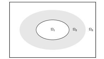
Figure 2: Two other ways of domain decomposition.

2.2 Classical SWR algorithm

The Schwarz methods being iterative, we label the iteration number of the algorithms by $k$ and denotes by $u_{j}^{k}$ the solution on subdomain $(0,T)\times\Omega_{j}$ at iteration $k=1,2,...$.

The classical SWR algorithm is given by

(2) $$\left\{\begin{array}[]{ll}\mathscr{L}u_{j}^{k}=0,&(t,x,y)\in(0,T)\times\Omega_{j},\\ u^{k}_{j}(0,x,y)=u_{0}(x,y),&(x,y)\in\Omega_{j},\\ B_{j}u_{j}^{k}=B_{j}u_{j-1}^{k-1},&x=a_{j},\\ B_{j}u_{j}^{k}=B_{j}u_{j+1}^{k-1},&x=b_{j},\\ \partial_{\mathbf{n}_{j}}u_{j}^{k}=0,&y=y_{l},y_{b},\end{array}\right.$$

with a special treatment for the two extreme subdomains $(0,T)\times\Omega_{1}$ and $(0,T)\times\Omega_{N}$ since the boundary conditions are imposed on $x=a_{1}$ and $x=b_{N}$

$$B_{1}u_{1}^{k}=(\partial_{\mathbf{n}}+S_{b})u_{1}^{k}=0,\ x=a_{1},\quad B_{N}u_{N}^{k}=(\partial_{\mathbf{n}}+S_{b})u_{N}^{k}=0,\ x=b_{N}.$$

The boundary condition at interface nodes $a_{j}$ and $b_{j}$ is given in term of operator $B_{j}$ defined by

(3) $$B_{j}=\partial_{\mathbf{n}_{j}}+S_{j},\ j=1,...,N,$$

where $S_{j}$ is a transmission operator. Various $S_{j}$ operators can be considered. The classical widely used Robin transmission condition is given by

(4) $$S_{j}=-ip,\ p\in\mathbb{R}^{+},\ j=1,2,...,N.$$

Traditionally, the optimal transmission operator is given in term of transparent boundary conditions. For the general linear two dimensional Schrödinger equation, we only have access to approximated version of the TBCs given by the recently constructed absorbing boundary condition $S_{\mathrm{pade}}^{m}$ [1, 2] which we used as the transmission condition

(5) $$S_{j}=-i\sqrt{i\partial_{t}+\Delta_{\Gamma_{j}}+V},\ j=1,2,...,N,$$

where $\Gamma_{1}=\{b_{1}\}\times(y_{b},y_{u})$, $\Gamma_{j}=\{a_{j},b_{j}\}\times(y_{b},y_{u}),j=2,3,...,N-1$ and $\Gamma_{N}=\{a_{N}\}\times(y_{b},y_{u})$. In our case, the Laplace–Beltrami operator $\Delta_{\Gamma_{j}}$ is $\partial_{y}^{2}$. Numerically, this operator is approximated by Padé approximation of order $m$

$$\sqrt{i\partial_{t}+\Delta_{\Gamma_{j}}+V}u\approx\Big{(}\sum_{s=0}^{m}a_{s}^{m}-\sum_{s=1}^{m}a_{s}^{m}d_{s}^{m}(i\partial_{t}+\Delta_{\Gamma_{j}}+V+d_{s}^{m})^{-1}\Big{)}u.$$

If the potential $V=0$ and the spatial domain is $\mathbb{R}^{2}$, the absorbing boundary condition is actually a transparent boundary conditions. Then it could be proven that the transmission condition $S_{\mathrm{pade}}^{m}$ leads to an optimal SWR method.

The classical SWR algorithm is initialized by an initial guess of $B_{j}u_{j}^{0}|_{x=a_{j},b_{j}}$, $j=1,2,...,N$. The boundary conditions for any subdomain $\Omega_{j}$ at iteration $k+1$ involve the knowledge of the values of the functions on adjacent subdomains $\Omega_{j-1}$ and $\Omega_{j+1}$ at prior iteration $k$. Thanks to the initial guess, we can solve the Schrödinger equation on each subdomain, allowing to build the new boundary conditions for the next step, communicating them to other subdomains. This procedure is summarized in (6) for $N=3$ subdomains at iteration $k$.

(6) $$\begin{pmatrix}B_{1}u_{1}^{k}|_{x=b_{1}}\\ B_{2}u_{2}^{k}|_{x=a_{2}}\\ B_{2}u_{2}^{k}|_{x=b_{2}}\\ B_{3}u_{3}^{k}|_{x=a_{3}}\end{pmatrix}\underrightarrow{\hskip 2.84544pt\text{\footnotesize{\emph{Solve}}}\hskip 2.84544pt}\begin{pmatrix}u_{1}^{k}\\ u_{2}^{k}\\ u_{3}^{k}\end{pmatrix}\rightarrow\begin{pmatrix}B_{2}u_{1}^{k}|_{x=b_{1}}\\ B_{1}u_{2}^{k}|_{x=a_{2}}\\ B_{3}u_{2}^{k}|_{x=b_{2}}\\ B_{2}u_{3}^{k}|_{x=a_{3}}\end{pmatrix}\underrightarrow{\hskip 2.84544pt\text{\footnotesize{\emph{Comm.}}}\hskip 2.84544pt}\begin{pmatrix}B_{1}u_{1}^{k+1}|_{x=b_{1}}\\ B_{2}u_{2}^{k+1}|_{x=a_{2}}\\ B_{2}u_{2}^{k+1}|_{x=b_{2}}\\ B_{3}u_{3}^{k+1}|_{x=a_{3}}\end{pmatrix}.$$

Let us define the flux at iteration $k$ by

$$g^{k}=(B_{1}u_{1}^{k}|_{x=b_{1}},\cdots,B_{j}u_{j}^{k}|_{x=a_{j}},B_{j}u_{j}^{k}|_{x=b_{j}},\cdots,B_{N}u_{N}^{k}|_{x=a_{N}})^{\top},$$

"$\cdot^{\top}$" denoting the transpose of the vector. Thanks to this definition, we give a new interpretation to the algorithm which can be written as

(7) $$g^{k+1}=\mathcal{R}_{c}g^{k},$$

where $\mathcal{R}_{c}$ is a linear operator. The solution to this iteration process is given as the solution to the continuous interface problem

(8) $$(I-\mathcal{R}_{c})g=0,\ g=\lim_{k\rightarrow\infty}g^{k}.$$

where $I$ is identity operator.

2.3 Classical DDS algorithm

The other algorithm we consider in this paper is the domain decomposition in space algorithm (DDS). The equation (1) is first semi-discretized in time on the entire domain $(0,T)\times\Omega$. The time interval $(0,T)$ is discretized uniformly with $N_{T}$ intervals of length $\Delta t$. We denotes $u_{n}$ (resp. $V_{n}$) an approximation of the solution $u$ (resp. $V$) at time $t_{n}=n\Delta t$. The Crank-Nicolson scheme on $(0,T)\times\Omega$ reads

$$i\frac{u_{n}-u_{n-1}}{\Delta t}+\Delta\frac{u_{n}+u_{n-1}}{2}+\frac{V_{n}+V_{n-1}}{2}\frac{u_{n}+u_{n-1}}{2}=0,\ 1\leqslant n\leqslant N_{T}.$$

By introducing new variables $v_{n}=(u_{n}+u_{n-1})/2$ with $v_{0}=u_{0}$ and $W_{n}=(V_{n}+V_{n-1})/2$, we get a stationary equation defined on $\Omega$ with unknown $v_{n}$

(9) $$\mathcal{L}_{\mathbf{x}}v_{n}=\frac{2i}{\Delta t}u_{n-1},$$

where $\mathcal{L}_{\mathbf{x}}:=\frac{2i}{\Delta t}+\Delta+W_{n}$. We recover the original unknown by $u_{n}=2v_{n}-u_{n-1}$. Then, the optimized Schwarz algorithm is applied to the stationary equation (9). We denote by $R_{j},j=1,2,...,N$ the restriction operator from $\Omega$ to $\Omega_{j}$. At time $t_{n}$, the classical algorithm reads

(10) $$\left\{\begin{array}[]{ll}\mathscr{L}_{\mathbf{x}}v_{n,j}^{k}=\frac{2i}{\Delta t}R_{j}u_{n-1},&(x,y)\in\Omega_{j},\\ \partial_{\mathbf{n}_{j}}v_{n,j}^{k}+\overline{S}_{j}v_{n,j}^{k}=\partial_{\mathbf{n}_{j}}v_{n,j-1}^{k-1}+\overline{S}_{j}v_{n,j-1}^{k-1},&x=a_{j},\\ \partial_{\mathbf{n}_{j}}v_{n,j}^{k}+\overline{S}_{j}v_{n,j}^{k}=\partial_{\mathbf{n}_{j}}v_{n,j+1}^{k-1}+\overline{S}_{j}v_{n,j+1}^{k-1},&x=b_{j},\\ \partial_{\mathbf{n}_{j}}v_{n,j}^{k}=0,&y=y_{l},y_{b},\end{array}\right.$$

where $v_{n,j}^{k}$ denotes the unknown at time $t_{n}$, on subdomain $\Omega_{j}$ at iteration $k$ and $\overline{S}_{j}$ is the semi-discrete form of $S_{j}$ given by (4) or (5). A special treatment for the two extreme subdomains is needed and the boundary conditions read $\partial_{\mathbf{n}_{1}}v_{n,1}^{k}+\overline{S}_{1}v_{n,1}^{k}=0,x=a_{1}$, $\partial_{\mathbf{n}_{N}}v_{n,N}^{k}+\overline{S}_{N}v_{n,N}^{k}=0,x=b_{N}$.

Since the interval $(t_{n-1},t_{n})$ contains only one time step, the DDS algorithm can be numerically interpreted as a sequence of some SWR algorithms.

The initial datum is $u_{0}$.

for $n=1,2,...,N_{T}$ do

       Apply the SWR algorithm to

$$\left\{\begin{array}[]{ll}\mathscr{L}u=0,\ (t,x,y)\in(t_{n-1},t_{n})\times\Omega,\\ u(0,x,y)=u_{n-1}(x,y),\ (x,y)\in\Omega,\\ \end{array}\right.$$

where $t_{n}=n\Delta t$.

Algorithm 1 DDS algorithm

3 Discrete interface problem

We know by (8) that the classical SWR algorithm reduces to the interface problem

$$(I-\mathcal{R}_{c})g=0,\ g=\lim_{k\rightarrow\infty}g^{k}.$$

The aim of this section is discretize this relation and to show that the discrete interface problem can be written as

(11) $$(I-\mathcal{L}_{h})\mathbf{g}=\mathbf{d},$$

where the vector $\mathbf{g}$ is the discrete form of $g$, $\mathbf{d}$ is a vector

$$\mathbf{d}=(\mathbf{d}_{1,r}^{\top},\mathbf{d}_{2,l}^{\top},\mathbf{d}_{2,r}^{\top},\cdots,\mathbf{d}_{N,l}^{\top})^{\top}\in\mathbb{R}^{N_{y}\times N_{T}},$$

and $\mathcal{L}_{h}$ is a block matrix (the notation “MPI $j$” above the columns of the matrix will be used in section 4)

(12) $$\mathcal{L}_{h}=\begin{pmatrix}\lx@intercol\overbrace{\hskip 20.00003pt}^{\mathrm{MPI}\ 0}\hfil\lx@intercol&\lx@intercol\overbrace{\hskip 50.00008pt}^{\mathrm{MPI}\ 1}\hfil\lx@intercol&\lx@intercol\overbrace{\hskip 50.00008pt}^{\mathrm{MPI}\ 2}\hfil\lx@intercol&&\lx@intercol\overbrace{\hskip 80.00012pt}^{\mathrm{MPI}\ N-2}\hfil\lx@intercol&\lx@intercol\overbrace{\hskip 20.00003pt}^{\mathrm{MPI}\ N-1}\hfil\lx@intercol\\ &X^{2,1}&X^{2,2}&&&\\ X^{1,4}\\ &&&X^{3,1}&X^{3,2}\\ &X^{2,3}&X^{2,4}\\ &&&&&\cdots\\ &&&X^{3,3}&X^{3,4}\\ &&&&&&X^{N-1,1}&X^{N-1,2}\\ &&&&&\cdots\\ &&&&&&&&X^{N,1}\\ &&&&&&X^{N-1,3}&X^{N-1,4}\end{pmatrix}.$$

The concrete definitions of $\mathbf{d}_{j,l}$, $\mathbf{d}_{j,r}$, $j=1,2,...,N$ and the bloks in $\mathcal{L}_{h}$ are given in proposition 3.5 and proposition 3.6. The subsection 3.2 is devoted to the derivation of some important properties of $\mathcal{L}_{h}$, which give the ground to make the new algorithm given in section 4.

3.1 Preliminaries related to discretization

Without loss of generality, we present the discretization of (1) on $(0,T)\times\Omega$ with the following boundary conditions [1, 2]

$$\left\{\begin{array}[]{ll}\partial_{\mathbf{n}}u=0,\ y=y_{b},y_{u},\\ \partial_{\mathbf{n}}u+Su=l(t,y),\ x=x_{l},\\ \partial_{\mathbf{n}}u+Su=r(t,y),\ x=x_{r},\end{array}\right.$$

where $l(t,y)$ and $r(t,y)$ are two functions. The discrete version of (2) follows immediately. Concerning the semi-discretization with respect to time, we follow the procedure given in section 2.3 for the classical DDS algorithm. The scheme therefore reads

(13) $$\frac{2i}{\Delta t}v_{n}+\Delta v_{n}+W_{n}v_{n}=\frac{2i}{\Delta t}u_{n-1}.$$

The semi-discrete transmission condition is given by

$$\partial_{\mathbf{n}}v_{n}+\overline{S}v_{n}=l_{n},\ x=x_{l},\quad\partial_{\mathbf{n}}v_{n}+\overline{S}v_{n}=r_{n},\ x=x_{r},$$

where $l_{n}=l(n\Delta t,y)$, $r_{n}=r(n\Delta t,y)$ and $\overline{S}$ is the semi-discrete form of $S$. If we consider the Robin transmission condition (4), we have

(14) $$\mathrm{Robin:}\quad\overline{S}v_{n}=-ip\cdot v_{n}.$$

The approximation of the transmission condition (5) is given by

(15) $$S_{\mathrm{pade}}^{m}:\quad\overline{S}v_{n}=-i\displaystyle\sum_{s=0}^{m}a_{s}^{m}v_{n}+i\sum_{s=1}^{m}a_{s}^{m}d_{s}^{m}\varphi^{n-1/2}_{s},$$

where $a_{s}^{m}=e^{i\theta/2}/(m\cos^{2}(\frac{(2s-1)\pi}{4m}))$, $d_{s}^{m}=e^{i\theta}\tan^{2}(\frac{(2s-1)\pi}{4m})$, $s=0,2,...,m$, $\theta=\frac{\pi}{4}$. The auxiliary functions $\varphi^{n-1/2}_{s}$, $s=1,2,...,m$ are defined as the solutions of the set of equations

$$\left\{\begin{aligned} &\big{(}\frac{2i}{\Delta t}+\Delta_{\Gamma}+W_{n}+d_{s}^{m}\big{)}\varphi^{n-1/2}_{s}-v_{n}=\frac{2i}{\Delta t}\varphi^{n-1}_{s},\\ &\varphi_{s}^{n}=2\varphi_{s}^{n-1/2}-\varphi_{s}^{n-1},\ \varphi_{s}^{0}=0.\end{aligned}\right.$$

The spatial approximation is realized by the standard $\mathbb{Q}_{1}$ finite element method. The uniform mesh size of a discrete element is $(\Delta x,\Delta y)$. We denote by $N_{x}$ (resp. $N_{y}$) the number of nodes in $x$ (resp. $y$) direction on each subdomain. Let us denote by $\mathbf{v}_{n}$ (resp. $\mathbf{u}_{n}$) the nodal interpolation vector of $v_{n}$ (resp. $u_{n}$), $\mathbf{l}_{n}$ (resp. $\mathbf{r}_{n}$) the nodal interpolation vector of $l_{n}$ (resp. $r_{n}$), $\mathbb{M}$ the mass matrix, $\mathbb{S}$ the stiffness matrix and $\mathbb{M}_{W_{n}}$ the generalized mass matrix with respect to $\int_{\Omega}W_{n}v\phi dx$. Let $\mathbb{M}^{\Gamma}$ the boundary mass matrix, $\mathbb{S}^{\Gamma}$ the boundary stiffness matrix and $\mathbb{M}^{\Gamma}_{W_{n}}$ the generalized boundary mass matrix with respect to $\int_{\Gamma}W_{n}v\phi d\Gamma$. We denote by $Q_{l}$ (resp. $Q_{r}$) the restriction operators (matrix) from $\Omega$ to $\{x_{l}\}\times(y_{b},y_{u})$ (resp. $\{x_{r}\}\times(y_{b},y_{u})$) and $Q^{\top}=(Q_{l}^{\top},Q_{r}^{\top})$. The matrix formulation for the transmission condition Robin is therefore given by

(16) $$\mathrm{Robin}:\quad\Big{(}\mathbb{A}_{n}+ip\cdot\mathbb{M}^{\Gamma}\Big{)}\mathbf{v}_{n}=\frac{2i}{\Delta t}\mathbb{M}\mathbf{u}_{n-1}-\mathbb{M}^{\Gamma}Q^{\top}\begin{pmatrix}\mathbf{l}_{n}\\ \mathbf{r}_{n}\end{pmatrix},$$

where $\mathbb{A}_{n}=\frac{2i}{\Delta t}\mathbb{M}-\mathbb{S}+\mathbb{M}_{W_{n}}$. The size of this linear system is $N_{x}\times N_{y}$. If we consider the transmission condition $S_{\mathrm{pade}}^{m}$, we have

$$\begin{pmatrix}\mathbb{A}_{n}+i(\sum_{s=0}^{m}a_{s}^{m})\cdot\mathbb{M}^{\Gamma}&\mathbb{B}_{1}&\mathbb{B}_{2}&\cdots&\mathbb{B}_{m}\\ \mathbb{C}&\mathbb{D}_{1}^{n}\\ \mathbb{C}&&\mathbb{D}_{2}^{n}\\ \vdots&&&\ddots\\ \mathbb{C}&&&&\mathbb{D}_{m}^{n}\end{pmatrix}\begin{pmatrix}\mathbf{v}_{n}\\ \bm{\varphi}^{n-1/2}_{1}\\ \bm{\varphi}^{n-1/2}_{2}\\ \vdots\\ \bm{\varphi}^{n-1/2}_{m}\end{pmatrix}$$

(17) $$=\begin{pmatrix}\mathbb{M}_{j}\\ &Q\mathbb{M}^{\Gamma}Q^{\top}\\ &&Q\mathbb{M}^{\Gamma}Q^{\top}\\ &&&\ddots\\ &&&&Q\mathbb{M}^{\Gamma}Q^{\top}\end{pmatrix}\begin{pmatrix}\mathbf{u}_{n-1}\\ \bm{\varphi}^{n-1}_{1}\\ \bm{\varphi}^{n-1}_{2}\\ \vdots\\ \bm{\varphi}^{n-1}_{m}\end{pmatrix}-\begin{pmatrix}\mathbb{M}^{\Gamma}Q^{\top}\begin{pmatrix}\mathbf{l}_{n}\\ \mathbf{r}_{n}\end{pmatrix}\\ 0\\ \vdots\\ 0\end{pmatrix},$$

with

$$\mathbb{B}_{s}=-ia_{s}^{m}d_{s}^{m}\mathbb{M}^{\Gamma}Q^{\top},\ 1\leqslant s\leqslant m,$$

$$\mathbb{C}=-Q\mathbb{M}^{\Gamma},$$

$$\mathbb{D}_{s}^{n}=Q(\frac{2i}{\Delta t}\mathbb{M}^{\Gamma}-\mathbb{S}^{\Gamma}+\mathbb{M}^{\Gamma}_{W_{n}}+d_{s}^{m}\mathbb{M}^{\Gamma})Q^{\top},\ 1\leqslant s\leqslant m.$$

It is a linear system with unknown $(\mathbf{v}_{n},\bm{\varphi}^{n-1/2}_{1},...,\bm{\varphi}^{n-1/2}_{m})$ where $\bm{\varphi}^{n-1/2}_{s}$ is the nodal interpolation of $\varphi^{n-1/2}_{s}$ on the boundary.

Remark 3.1.

The $S_{\mathrm{pade}}^{m}$ transmission condition involves a larger linear system to solve than the one of the Robin transmission condition. The cost of the algorithm with the $S_{\mathrm{pade}}^{m}$ transmission condition is therefore more expensive.

The equations (16) and (17) are given for a fixed discrete time $t_{n}$. They however can be written globally in time by some straightforward calculations.

Proposition 3.2.

For the Robin transmission condition, the global form in time of the equation (16) is

(18) $$(\mathbf{A}-\mathbf{B})\mathbf{v}=\mathbf{F}-\mathbf{M}^{\Gamma}\mathbf{Q}^{\top}\mathbf{g},$$

where $\mathbf{B}=-ip\cdot\mathbf{M}^{\Gamma}=-ip\cdot\mathrm{diag}_{N_{T}}\{\mathbb{M}^{\Gamma}\}$, $\mathbf{Q}_{l}^{\top}=\mathrm{diag}_{N_{T}}\{Q_{l}^{\top}\}$, $\mathbf{Q}_{r}^{\top}=\mathrm{diag}_{N_{T}}\{Q_{r}^{\top}\}$ and

$$\mathbf{A}=\begin{pmatrix}\mathbb{A}_{1}&&&&\\ -\frac{4i}{\Delta t}\mathbb{M}&\mathbb{A}_{2}&&&\\ \frac{4i}{\Delta t}\mathbb{M}&-\frac{4i}{\Delta t}\mathbb{M}&\mathbb{A}_{3}&&&\\ \vdots&\vdots&&\ddots&\\ &&&-\frac{4i}{\Delta t}\mathbb{M}&\mathbb{A}_{N_{T}}\end{pmatrix},\ \mathbf{v}=\begin{pmatrix}\mathbf{v}_{1}\\ \mathbf{v}_{2}\\ \vdots\\ \vdots\\ \mathbf{v}_{N_{T}}\end{pmatrix},$$

$$\mathbf{F}=\frac{2i}{\Delta t}\begin{pmatrix}\mathbb{M}\mathbf{u}_{0}\\ -\mathbb{M}\mathbf{u}_{0}\\ \vdots\\ (-1)^{N_{T}-1}\mathbb{M}\mathbf{u}_{0}\end{pmatrix},\ \mathbf{Q}^{\top}=\begin{pmatrix}Q_{l}^{\top}&&&&Q_{r}^{\top}\\ &Q_{l}^{\top}&&&&Q_{r}^{\top}\\ &&\ddots&&&&\ddots\\ &&&Q_{l}^{\top}&&&&Q_{r}^{\top}\end{pmatrix}.$$

Proposition 3.3.

If we consider the transmission condition $S_{\mathrm{pade}}^{m}$, then the equation (17) can be written globally in time as (18)

$$(\mathbf{A}-\mathbf{B})\mathbf{v}=\mathbf{F}-\mathbf{M}^{\Gamma}\mathbf{Q}^{\top}\mathbf{g},$$

with $\mathbf{B}$ given by

(19) $$\mathbf{B}=-\begin{pmatrix}c_{a}\mathbb{M}^{\Gamma}+\mathbb{Y}^{1,1}\\ \mathbb{Y}^{2,1}&c_{a}\mathbb{M}^{\Gamma}+\mathbb{Y}^{2,2}\\ \mathbb{Y}^{3,1}&\mathbb{Y}^{3,1}&c_{a}\mathbb{M}^{\Gamma}+\mathbb{Y}^{3,3}\\ \vdots&\vdots&&\ddots\\ \mathbb{Y}^{N_{T},1}&\mathbb{Y}^{N_{T},2}&\mathbb{Y}^{N_{T},3}&\cdots&c_{a}\mathbb{M}^{\Gamma}+\mathbb{Y}^{N_{T},N_{T}}\end{pmatrix},$$

where $c_{a}=i(\sum_{s=0}^{m}a_{s}^{m})$.

Proof.

According to (17), for $s=1,2,...,m$, $n=1,2,...,N_{T}$, we have

$$-Q\mathbb{M}^{\Gamma}\mathbf{v}_{n}+\mathbb{D}_{s}^{n}\bm{\varphi}_{s}^{n-1/2}=\frac{2i}{\Delta t}Q_{j}\mathbb{M}^{\Gamma}Q^{\top}\bm{\varphi}_{s}^{n-1},\ \ n\geqslant 1,$$

where $\mathbb{D}_{s}^{n}=Q(\frac{2i}{\Delta t}\mathbb{M}^{\Gamma}-\mathbb{S}^{\Gamma}+\mathbb{M}^{\Gamma}_{W_{n}}+d_{s}^{m}\mathbb{M}^{\Gamma})Q^{\top}$. We therefore obtain

$$\bm{\varphi}_{s}^{n-1/2}=(\mathbb{D}_{s}^{n})^{-1}Q_{j}\mathbb{M}^{\Gamma}\mathbf{v}_{n}+(\mathbb{D}_{s}^{n})^{-1}\frac{2i}{\Delta t}Q\mathbb{M}^{\Gamma}Q^{\top}\bm{\varphi}_{s}^{n-1},$$

and

$$\bm{\varphi}_{s}^{n-1}=2\bm{\varphi}_{s}^{n-3/2}-\bm{\varphi}_{s}^{n-2},\ \bm{\varphi}_{s}^{0}=0,\ n\geqslant 2.$$

By induction, $\bm{\varphi}_{s}^{n-1/2}$ is given by

(20) $$\bm{\varphi}_{s}^{n-1/2}=\sum_{p=1}^{n}\mathbb{L}_{s}^{n,p}\mathbf{v}_{p},$$

where $\mathbb{L}_{s}^{n,p}$ are matrix. Replacing $\bm{\varphi}_{s}^{n-1/2}$ by $\mathbf{v}_{p}$ in the first row of the equation (17) gives

(21) $$\Big{(}\mathbb{A}_{n}+i(\sum_{s=0}^{m}a_{s}^{m})\cdot\mathbb{M}^{\Gamma}\Big{)}\mathbf{v}_{n} +\sum_{p=1}^{n}\mathbb{Y}^{n,p}\mathbf{v}_{p}=\frac{2i}{\Delta t}\mathbb{M}\mathbf{u}_{n-1}-\mathbb{M}^{\Gamma}Q^{\top}\begin{pmatrix}\mathbf{l}_{n}\\ \mathbf{r}_{n}\end{pmatrix},$$

where $\mathbb{Y}^{n,p}:=-i\sum_{s=1}^{m}a_{s}^{m}d_{s}^{m}\mathbb{M}^{\Gamma}Q^{\top}\mathbb{L}_{s}^{n,p}$ Then, according to (21), the matrix $\mathbf{B}$ is given by (19).

Remark 3.4.

Following the same procedure, the equation (2) is discretized on each subdomain $(0,T)\times\Omega_{j}$. Accordingly, we define the matrices $\mathbf{A}_{j}$, $\mathbf{B}_{j}$, $\mathbf{M}^{\Gamma_{j}}$, $\mathbb{L}_{j,s}^{n,p}$ associated with the finite element method, the restriction matrix $\mathbf{Q}_{j,l}$, $\mathbf{Q}_{j,r}$ and the solution vector $\mathbf{v}_{j,n}^{k}$. The subscript "$j$" emphasizes the definition of the matrices associated to the subdomains $(0,T)\times\Omega_{j}$.

3.2 Properties of $\mathcal{L}_{h}$

Let us define the fluxes

$$l_{j}^{k}(t,y)=\partial_{\mathbf{n}_{j}}v^{k}_{j}+S_{j}v^{k}_{j},\ r_{j}^{k}(t,y)=\partial_{\mathbf{n}_{j}}v^{k}_{j}+S_{j}v^{k}_{j},\ (t,y)\in(0,T)\times\Omega_{j},$$

for $j=1,2,...,N$ with the two special cases $l_{1}^{k}=r_{N}^{k}=0$ corresponding to the left and right boundaries and

$$l_{n,j}^{k}=l_{j}^{k}(t_{n},y),\ r_{n,j}^{k}=r_{j}^{k}(t_{n},y).$$

We denote by $\mathbf{l}_{j,n}^{k}$ (resp. $\mathbf{r}_{j,n}^{k}$) the nodal interpolation vector of $l_{j,n}^{k}$ (resp. $r_{j,n}^{k}$)

(22) $$\quad\left\{\begin{aligned} &\mathbf{r}_{j-1,n}^{k+1}=-\mathbf{l}_{j,n}^{k}+2Q_{j,l}\cdot\widetilde{S}_{j}\mathbf{v}_{j,n}^{k},\ j=2,3,...,N,\\ &\mathbf{l}_{j+1,n}^{k+1}=-\mathbf{r}_{j,n}^{k}+2Q_{j,r}\cdot\widetilde{S}_{j}\mathbf{v}_{j,n}^{k},\ j=1,2,...,N-1,\end{aligned}\right.$$

where we have for the Robin transmission condition

$$\mathrm{Robin:}\quad\widetilde{S}_{j}\mathbf{v}_{j,n}^{k}=-ip\cdot\mathbf{v}_{j,n}^{k},$$

and for the $S_{\mathrm{pade}}^{m}$ condition

$$S_{\mathrm{pade}}^{m}:\quad\widetilde{S}_{j}\mathbf{v}_{j,n}^{k}=-i(\sum_{s=0}^{m}a_{s}^{m})\mathbf{v}_{j,n}^{k}+i\sum_{s=1}^{m}a_{s}^{m}d_{s}^{m}\bm{\varphi}^{n-1/2}_{j,s}.$$

Then, we define the discrete interface vector $\mathbf{g}$ by

(23) $$\mathbf{g}=\lim_{k\rightarrow\infty}\mathbf{g}^{k},$$

where

$$\mathbf{g}^{k}=(\mathbf{g}_{1}^{k,\top},\mathbf{g}_{2}^{k,\top},...,\mathbf{g}_{N}^{k,\top})^{\top},$$

$$\mathbf{g}_{1}^{k}=(\mathbf{r}_{1,1}^{k,\top},\mathbf{r}_{1,2}^{k,\top},\cdots,\mathbf{r}_{1,N_{T}}^{k,\top})^{\top}\in\mathbb{C}^{N_{y}\times N_{T}},$$

$$\mathbf{g}_{N}^{k}=(\mathbf{l}_{N,1}^{k,\top},\mathbf{l}_{N,2}^{k,\top},\cdots,\mathbf{l}_{N,N_{T}}^{k,\top})^{\top}\in\mathbb{C}^{N_{y}\times N_{T}},$$

$$\mathbf{g}_{j}^{k}=(\mathbf{l}_{j,1}^{k,\top},\cdots,\mathbf{l}_{j,N_{T}}^{k,\top},\mathbf{r}_{j,1}^{k,\top},\cdots,\mathbf{r}_{j,N_{T}}^{k,\top})^{\top}\in\mathbb{C}^{2N_{y}\times N_{T}},\ j=2,3,...N-1.$$

Proposition 3.5.

If we consider the Robin transmission condition, the discrete form of the interface problem (8) is given by (11).

Proof.

According to (22), and the definitions of $\mathbf{g}^{k}$, it is easy to verify that

(24) $$X^{j,1}=-I-2ip\cdot\mathbf{Q}_{j,l}(\mathbf{A}_{j}-\mathbf{B}_{j})^{-1}\mathbf{M}^{\Gamma_{j}}\mathbf{Q}_{j,l}^{\top},$$

$$X^{j,2}=-2ip\cdot\mathbf{Q}_{j,l}(\mathbf{A}_{j}-\mathbf{B}_{j})^{-1}\mathbf{M}^{\Gamma_{j}}\mathbf{Q}_{j,r}^{\top},$$

$$X^{j,3}=-2ip\cdot\mathbf{Q}_{j,r}(\mathbf{A}_{j}-\mathbf{B}_{j})^{-1}\mathbf{M}^{\Gamma_{j}}\mathbf{Q}_{j,l}^{\top},$$

$$X^{j,4}=-I-2ip\cdot\mathbf{Q}_{j,r}(\mathbf{A}_{j}-\mathbf{B}_{j})^{-1}\mathbf{M}^{\Gamma_{j}}\mathbf{Q}_{j,r}^{\top},$$

and

(25) $$\begin{split}\mathbf{d}_{j,l}&=2ip\cdot\mathbf{Q}_{j-1,r}(\mathbf{A}_{j-1}-\mathbf{B}_{j-1})^{-1}\mathbf{F}_{j-1},\ j=2,3,...,N,\\ \mathbf{d}_{j,r}&=2ip\cdot\mathbf{Q}_{j+1,l}(\mathbf{A}_{j+1}-\mathbf{B}_{j+1})^{-1}\mathbf{F}_{j+1},\ j=1,2,...,N-1.\end{split}$$

Proposition 3.6.

If we consider the transmission condition $S_{\mathrm{pade}}^{m}$, then (11) is the discrete form of the interface problem (8).

Proof.

By using (22), we have

$$\widetilde{S}_{j}\mathbf{v}_{j,n}^{k}=-c_{a}\mathbf{v}_{j,n}^{k}+i\sum_{s=1}^{m}a_{s}^{m}d_{s}^{m}\sum_{p=1}^{n}\mathbb{L}_{j,s}^{n,p}\mathbf{v}_{j,p}^{k}=-c_{a}\mathbf{v}_{j,n}^{k}+i\sum_{p=1}^{n}\big{(}\sum_{s=1}^{m}a_{s}^{m}d_{s}^{m}\mathbb{L}_{j,s}^{n,p}\big{)}\mathbf{v}_{j,p}^{k}.$$

We could easily verify that

(26) $$X^{j,1}=-I+2\mathbf{Q}_{j,l}\mathbf{B}_{j}^{S}(\mathbf{A}_{j}-\mathbf{B}_{j})^{-1}\mathbf{M}^{\Gamma_{j}}\mathbf{Q}_{j,l}^{\top},$$

$$X^{j,2}=2\mathbf{Q}_{j,l}\mathbf{B}_{j}^{S}(\mathbf{A}_{j}-\mathbf{B}_{j})^{-1}\mathbf{M}^{\Gamma_{j}}\mathbf{Q}_{j,r}^{\top},$$

$$X^{j,3}=2\mathbf{Q}_{j,r}\mathbf{B}_{j}^{S}(\mathbf{A}_{j}-\mathbf{B}_{j})^{-1}\mathbf{M}^{\Gamma_{j}}\mathbf{Q}_{j,l}^{\top},$$

$$X^{j,4}=-I+2\mathbf{Q}_{j,r}\mathbf{B}_{j}^{S}(\mathbf{A}_{j}-\mathbf{B}_{j})^{-1}\mathbf{M}^{\Gamma_{j}}\mathbf{Q}_{j,r}^{\top},$$

and

(27) $$\begin{split}\mathbf{d}_{j,l}&=\mathbf{Q}_{j-1,r}\mathbf{B}_{j-1}^{S}(\mathbf{A}_{j-1}-\mathbf{B}_{j-1})^{-1}\mathbf{F}_{j-1},\ j=2,3,...,N,\\ \mathbf{d}_{j,r}&=\mathbf{Q}_{j+1,l}\mathbf{B}_{j+1}^{S}(\mathbf{A}_{j+1}-\mathbf{B}_{j+1})^{-1}\mathbf{F}_{j+1},\ j=1,2,...,N-1,\end{split}$$

where the matrix $\mathbf{B}_{j}^{S}$ is defined by

$$\mathbf{B}_{j}^{S}=\begin{pmatrix}-c_{a}I+\displaystyle i\sum_{s=1}^{m}a_{s}^{m}d_{s}^{m}\mathbb{L}_{j,s}^{1,1}\\ \displaystyle i\sum_{s=1}^{m}a_{s}^{m}d_{s}^{m}\mathbb{L}_{j,s}^{2,1}&\displaystyle-c_{a}I+i\sum_{s=1}^{m}a_{s}^{m}d_{s}^{m}\mathbb{L}_{j,s}^{2,2}\\ \vdots&\vdots&\ddots\\ \displaystyle i\sum_{s=1}^{m}a_{s}^{m}d_{s}^{m}\mathbb{L}_{j,s}^{N_{T},1}&\displaystyle i\sum_{s=1}^{m}a_{s}^{m}d_{s}^{m}\mathbb{L}_{j,s}^{N_{T},2}&\cdots&-c_{a}I+\displaystyle i\sum_{s=1}^{m}a_{s}^{m}d_{s}^{m}\mathbb{L}_{j,s}^{N_{T},N_{T}}\end{pmatrix}.$$

Let us now study the structure of the subblock of $\mathcal{L}_{h}$ for time independent potential $V=V(x,y)$. More specifically, we focus on

(28) $$X^{1,4}=\{x^{1,4}_{n,s}\}_{1\leqslant n,s\leqslant N_{T}},$$

$$X^{j,1}=\{x^{j,1}_{n,s}\}_{1\leqslant n,s\leqslant N_{T}},X^{j,2}=\{x^{j,2}_{n,s}\}_{1\leqslant n,s\leqslant N_{T}},$$

$$X^{j,3}=\{x^{j,3}_{n,s}\}_{1\leqslant n,s\leqslant N_{T}},X^{j,4}=\{x^{j,4}_{n,s}\}_{1\leqslant n,s\leqslant N_{T}},j=2,3,...,N-1,$$

$$X^{N,1}=\{x^{N,1}_{n,s}\}_{1\leqslant n,s\leqslant N_{T}}.$$

where $x^{j,1}_{n,s},x^{j,2}_{n,s},x^{j,3}_{n,s},x^{j,4}_{n,s}\in\mathbb{C}^{N_{y}\times N_{y}}$ are submatrices.

Each subblock $X_{j}^{1,2,3,4}$ are made of submatrices which are set on very specific positions. This structure is presented in Figure 3 for 3 time steps and 6 nodes on the interface between two subdomains. We see that each sub-diagonal block is identical. We present this property mathematically in proposition 3.7 with the two transmission condition Robin or $S_{\mathrm{pade}}^{m}$. The demonstration is similar to the one obtained for one dimensional Schrödinger equation [5]. The formal difference between dimension one and dimension two is that the flux are scalar in one dimension and vectors in two dimensions.

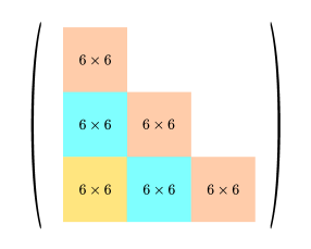
Figure 3: Block structure, $N_{T}=3$, $N_{y}=6$.

Proposition 3.7.

For the transmission Robin (resp. $S_{\mathrm{pade}}^{m}$), assuming that the linear system (16) (resp. (17)) is not singular, if the potential is time independent $V=V(x,y)$, then the matrices $X^{1,4}$, $X^{j,1}$,$X^{j,2}$, $X^{j,3}$, $X^{j,4}$, $j=2,3,...,N-1$ and $X^{N,1}$ are block lower triangular matrices and they satisfy

$$\begin{split}&x^{1,4}_{n,s}=x^{1,4}_{n-1,s-1},\\ &x^{j,1}_{n,s}=x^{j,1}_{n-1,s-1},\ x^{j,2}_{n,s}=x^{j,2}_{n-1,s-1},\\ &x^{j,3}_{n,s}=x^{j,3}_{n-1,s-1},\ x^{j,4}_{n,s}=x^{j,4}_{n-1,s-1},j=2,3,...,N-1,\\ &x^{N,1}_{n,s}=x^{N,1}_{n-1,s-1},\end{split}$$

for $2\leqslant s\leqslant n\leqslant N_{T}$.

If the potential is constant, the sub-blocks of $\mathcal{L}_{h}$ are simpler and follow the following proposition.

Proposition 3.8.

Assuming that the matrix $\mathbf{A}_{j}-\mathbf{B}_{j}$ is not singular with the Robin or the $S_{\mathrm{pade}}^{m}$ transmission condition, and that the mesh is uniform and the size of subdomains $\Omega_{j}$ are equal, if the potential $V$ is constant, then the subblocks of $\mathcal{L}_{h}$ satisfy

(29) $$X^{2,1}=X^{3,1}=\cdots=X^{N,1},\quad\ X^{2,2}=X^{3,2}=\cdots=X^{N-1,2},$$

$$X^{2,3}=X^{3,3}=\cdots=X^{N-1,3},\ X^{1,4}=X^{2,4}=\cdots=X^{N-1,4}.$$

Proof.

Thanks to the hypothesis of the proposition, the geometry of each subdomain is identical. Thus, the various matrices coming from the assembly of the finite element methods are the same. Therefore, we have

$$\mathbb{A}_{1}=\mathbb{A}_{2}=\cdots=\mathbb{A}_{N},\ \mathbb{M}^{\Gamma_{1}}=\mathbb{M}^{\Gamma_{2}}=\cdots=\mathbb{M}^{\Gamma_{N}},$$

and the restrictions matrices satisfy

$$Q_{1,l}=Q_{2,l}=\cdots=Q_{N,l},\ Q_{1,r}=Q_{2,r}=\cdots=Q_{N,r}.$$

Since $V$ is constant, then $\mathbb{M}_{1,W_{n}}=\mathbb{M}_{2,W_{n}}=...=\mathbb{M}_{N,W_{n}}$. Thus by definitions, we have

$$\mathbf{A}_{1}=\mathbf{A}_{2}=\cdots=\mathbf{A}_{N},\ \mathbf{B}_{1}=\mathbf{B}_{2}=\cdots=\mathbf{B}_{N},\ \mathbf{Q}_{1}=\mathbf{Q}_{2}=\cdots=\mathbf{Q}_{N},$$

and $\mathbf{B}_{1}^{S}=\mathbf{B}_{2}^{S}=\cdots=\mathbf{B}_{N}^{S}$ for the transmission condition $S_{\mathrm{pade}}^{m}$. The conclusion therefore follows from (24) and (26).

4 New algorithms for the Schrödinger equation with a constant potential

Thanks to the analysis yielded in previous section, we can build explicitly the interface problem (11). The main idea of our new algorithm is therefore to explicitly construct the matrix $\mathcal{L}_{h}$ and the vector $d$. Following propositions (3.7) and (3.8), it is sufficient to compute four subblocks to explicitly build the matrix $\mathcal{L}_{h}$. Without loss of generality, we construct the blocks $X^{2,1}$, $X^{2,2}$, $X^{2,3}$ and $X^{2,4}$. Furthermore, only the first $N_{y}$ columns of each block are necessarily computed.

4.1 New SWR algorithm

We propose here a new SWR algorithm for the Schrödinger equation with a constant potential $V$. We always suppose that the size of each subdomain is identical and the mesh is uniform.

1:  Build $\mathcal{L}_{h}$ and $d$ in relation $(I-\mathcal{L}_{h})\mathbf{g}=d$ explicitly.

2:  Solve the linear system $(I-\mathcal{L}_{h})\mathbf{g}=d$ by an iterative method (fixed point method or Krylov methods).

3:  Solve the Schrödinger equation on each subdomain on $(0,T)\times\Omega_{j}$ using the flux obtained from step 2.

Algorithm 2 New SWR algorithm, constant potential $V$

Mathematically, this new SWR algorithm is identical to the classical one. The main novelty here is that we construct explicitly the matrix $\mathcal{L}_{h}$ and the vector $d$ (corresponding to the first step), while in the classical algorithm, $\mathcal{L}_{h}$ remains an abstract operator. It is not usual to build explicitly such huge operator, but as we will see, its computation is not costly.

We show below the construction of $\mathcal{L}_{h}$ and $d$ for the Robin transmission condition. This is is based on the formulas (24) and (25). For the transmission condition $S_{\mathrm{pade}}^{m}$, the idea is similar, but involves (26) and (27). According to the proposition 3.5, the column $s$ of $X^{2,1}$ and $X^{2,3}$ are

$$\begin{split}X^{2,1}\mathbf{e}_{s}&=-\mathbf{e}_{s}-2ip\cdot\mathbf{Q}_{2,l}\mathbf{M}^{\Gamma_{2}}\mathbf{Q}_{2,l}^{\top}\mathbf{M}^{\Gamma_{2}}\mathbf{Q}_{2,l}^{\top}\mathbf{e}_{s},\\ X^{2,3}\mathbf{e}_{s}&=-2ip\cdot\mathbf{Q}_{2,r}(\mathbf{A}_{2}-\mathbf{B}_{2})^{-1}\mathbf{M}^{\Gamma_{2}}\mathbf{Q}_{2,l}^{\top}\mathbf{e}_{s},\end{split}$$

where the vector $\mathbf{e}_{s}=(0,0,...,1,...0)\in\mathbb{C}^{N_{T}\times N_{y}}$, all its elements being zero to the exception of the $s$-th, which is one. The element $\mathbf{M}^{\Gamma_{2}}\mathbf{Q}_{2,l}^{\top}\mathbf{e}_{s}$ being a vector, it is necessary to compute one time the application of $(\mathbf{A}_{2}-\mathbf{B}_{2})^{-1}$ to a vector. Similarly, we have

$$\begin{split}X^{2,2}\mathbf{e}_{s}&=-2ip\cdot\mathbf{Q}_{2,l}(\mathbf{A}_{2}-\mathbf{B}_{2})^{-1}\mathbf{M}^{\Gamma_{2}}\mathbf{Q}_{2,r}^{\top}\mathbf{e}_{s},\\ X^{2,4}\mathbf{e}_{s}&=-\mathbf{e}_{s}-2ip\cdot\mathbf{Q}_{2,r}(\mathbf{A}_{2}-\mathbf{B}_{2})^{-1}\mathbf{M}^{\Gamma_{2}}\mathbf{Q}_{2,r}^{\top}\mathbf{e}_{s},\end{split}$$

In conclusion, to know the first $N_{y}$ columns of $X^{2,1}$, $X^{2,2}$, $X^{2,3}$ and $X^{2,4}$, it is sufficient to compute $2N_{y}$ times the application of $(\mathbf{A}_{2}-\mathbf{B}_{2})^{-1}$ to a vector. In other words, this amounts to solve the Schrödinger equation on a single subdomain $2N_{y}$ times to build the matrix $\mathcal{L}_{h}$. Without loss of generality, since the geometry of each sub domain is identical and the matrix $\mathcal{L}_{h}$ is independent of the initial solution, we focus here on the domain $(0,T)\times\Omega_{2}$. The resolutions being all independent, we can solve them on different processors using MPI paradigm. We fix one MPI process per domain. To construct the matrix $\mathcal{L}_{h}$, we use the $N$ MPI processes to solve the equation on a single subdomain ($(0,T)\times\Omega_{2}$) $2N_{y}$ times. Each MPI process therefore solves the Schrödinger equation on a single subdomain maximum

$$N_{\mathrm{mpi}}:=[\frac{2N_{y}}{N}]+1\ \text{times,}$$

where $[x]$ denotes the integer part of $x$. This construction is therefore super-scalable in theory. Indeed, if $N$ is doubled, then the size of the subdomains is divided by two and $N_{\mathrm{mpi}}$ is also approximately halved.

Concerning the computational phase, the transposed matrix of $\mathcal{L}_{h}$ is stored in a distributed manner using the PETSc library [4]. As shown by (12), the first block column of $\mathcal{L}_{h}$ lies in MPI process 0. The second and third blocks columns are in MPI process 1, and so on for other processes. The size of each block is $(N_{T}\times N_{y})\times(N_{T}\times N_{y})$. Each block contains $(N_{T}+1)\times N_{T}/2\times N_{y}^{2}$ nonzero elements.

The construction of the vector $\mathbf{d}$ is similar. According to (25), one needs to apply $(\mathbf{A}_{j}-\mathbf{B}_{j})^{-1}$ to vector $\mathbf{F}_{j}$ for $j=1,2,...,N$. In other words, we solve the Schrödinger equation on each subdomain one time. Again, the vector is stored in a distributed manner using the PETSc library.

$$\mathbf{d}=2\begin{pmatrix}\mathbf{d}_{1,r}\\ \vdots\\ \mathbf{d}_{j,l}\\ \mathbf{d}_{j,r}\\ \vdots\\ \mathbf{d}_{N,l}\end{pmatrix}\begin{array}[]{c}\rdelim\}{1}{4pt}[MPI0,$N_T\times N_y$elements]\\ \\ \rdelim\}{2}{4pt}[MPI$j$,$2N_T\times N_y$elements]\\ \\ \\ \rdelim\}{1}{4pt}[MPI$N$,$N_T\times N_y$elements]\\ \end{array}$$

4.2 New DDS algorithm

Since we have interpreted the DDS method as sequence of some SWR methods in Algorithm 1, we can apply directly the ideas developped in the previous sections to the DDS method. Let us denote the interface problem of

$$\left\{\begin{array}[]{ll}i\partial_{t}u+\Delta u+Vu=0,&(t,x,y)\in(t_{n-1},t_{n})\times\Omega,\\ u(0,x,y)=u_{n-1}(x,y),&(x,y)\in\Omega,\\ \end{array}\right.$$

by

(30) $$(I-\mathcal{L}_{h,n})\mathbf{g}_{n}=d_{n},$$

where $\mathcal{L}_{h,n}$ is interface matrix and $d_{n}$ is vector. In the classical algorithm, $\mathcal{L}_{h,n}$ remains an abstract operator. We propose to build it explicitly in the new DDS algorithm. Actually, thanks to the following proposition, the computation of the complete operator $\mathcal{L}_{h,n}$ only require to compute $\mathcal{L}_{h,1}$.

Proposition 4.1.

For the transmission Robin and $S_{\mathrm{pade}}^{m}$, the interface matrix satisfies

$$\mathcal{L}_{h,1}=\mathcal{L}_{h,2}=...=\mathcal{L}_{h,N_{T}}.$$

Proof.

According to (24) and (26), the interface matrix is independent of the initial datum, thus the conclusion follows directly.

1: Build $\mathcal{L}_{h,1}$ explicitly.

2: The initial datum is $u_{0}$.

for $n=1,2,...,N_{T}$ do

       2.1: Build $d_{n}$ on time $t_{n}$,

       2.2: Solve the linear system $(I-\mathcal{L}_{h,n})\mathbf{g}_{h,n}=d_{n}$ by an iterative method, where the initial vector is chosen as $\mathbf{g}_{h,n-1}$.

       2.3: Solve the Schrödinger equation on each subdomain $(t_{n-1},t_{n})\times\Omega_{j}$ using the flux from step 2.2 to compute $u_{n}$.

Algorithm 3 New DDS algorithm, constant potential $V$

Mathematically, this new DDS algorithm is identical to the classical one. Compared with the new SWR algorithm, the construction of the interface matrix is less costly since the size of $\mathcal{L}_{h,1}$ is smaller than that of $\mathcal{L}_{h}$.

5 Preconditioned algorithms for general linear potential

In the case of a non constant potential, the proposition 3.8 does not hold. Thus we could not construct easily the matrix $\mathcal{L}_{h}$. The aim of this section is to present preconditioned algorithms for the Schrödinger equation (1) with a non constant potential $V=V(t,x,y)$. Adding a preconditioner to the equation (11) leads to a preconditioned SWR algorithm

(31) $$P^{-1}(I-\mathcal{L}_{h})\mathbf{g}=P^{-1}d,$$

We propose here to use

$$P=I-\mathcal{L}_{0},$$

where $\mathcal{L}_{0}$ denotes the interface matrix in (11) defined for the free Schrödinger equation when $V=0$. As mentioned in the previous section, it could be easily constructed numerically and it is stored in a distributed manner. For any vector $y$, the vector $x:=P^{-1}y$ is computed by solving the linear system

$$Px=y.$$

with Krylov methods (for example GMRES or BiCGStab). However, the size of $P$ increases linearly with the number of subdomains $N$. Also the number of involved operations for multiplying $\mathcal{L}_{0}$ and a vector (which is the basic operation of Krylov method) is not negligible compared to the computation of the solutions to the equations on each subdomain if $N$ is large. Thus, the application of the preconditioner increases.

We could derive straightforwardly a preconditioned DDS algorithm from the point of view of Algorithm 1. The preconditioner for all time steps $n=1,2,...,N_{T}$ is always chosen as

$$P=I-\mathcal{L}_{0,1},$$

where $\mathcal{L}_{0,1}$ is the interface matrix of (30) defined for $V=0$ and $n=1$.

Remark 5.1.

The idea of these new algorithm are not limited to the Schrödinger equation. It could also be applied to some other PDEs, like heat equation etc. The only limitation is that the mesh and the decomposition should be uniform.

6 Numerical results

The complete domain $\Omega=(-16,16)\times(-8,8)$ is decomposed into $N$ equal subdomains. The size of a single cell is $\Delta x\times\Delta y$. We consider two different meshes

$$\Delta x=1/128,\ \Delta y=1/8;$$

$$\Delta x=1/2048,\ \Delta y=1/128.$$

With the first mesh, it is possible to solve the Schrödinger equation (1) on the entire domain on a single node of a cluster composed of 92 nodes (16 cores/node, Intel Sandy Bridge E5-2670, 32GB memory/node). Thus we could observe if the parallel algorithms allow to reduce the total computation time of the sequential algorithm. We are interested in the strong scalability up to 1024 subdomains. The initial datum in this section is

(32) $$u_{0}(x,y)=e^{-x^{2}-y^{2}-0.5ix}.\quad\text{(see Figure \ref{Solinit0})}$$

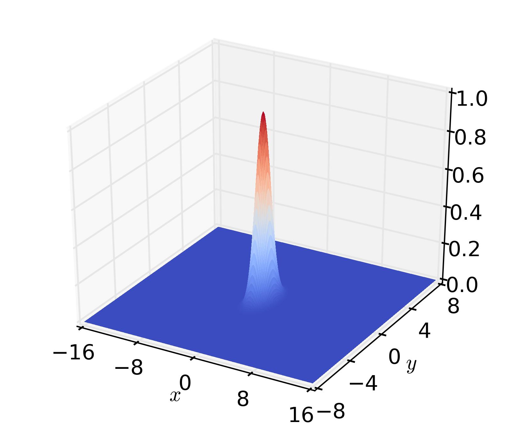
Figure 4: Initial datum $|u_{0}|$, $u_{0}=e^{-x^{2}-y^{2}-0.5ix}$.

This section is composed of two subsections. The first one is devoted to the free Schrödinger equation ($V=0$). In the second, we consider the Schrödinger equation with a linear potential $V=x^{2}+y^{2}$.

Remark 6.1.

For the DDS algorithm, we consider mostly the convergence properties (for example the number of iterations) of the first time step. In other words, we only study the evolution between $t^{0}\rightarrow t^{1}$ to compute $v^{1}$ with the optimized Schwarz method.

Remark 6.2.

The theoretical optimal parameter $p$ in the Robin transmission condition is not at hand for us. We then seek for the best parameter numerically for each case.

6.1 The free Schrödinger equation

In this part, we first compare the SWR method and the DDS algorithm. The DDS algorithm being more efficient, we next compare the classical DDS and the new DDS algorithms. Finally, the influence of parameters is studied in Section 6.1.3.

6.1.1 SWR vs. DDS

We compare the SWR and the DDS methods in the framework of the classical algorithm. The time step is set to $\Delta t=0.01$. The mesh size is $\Delta x=1/128$, $\Delta y=1/8$. Both methods are applied on time-space domain $(0,T)\times\Omega$ with various final time $T$. We denote by $N_{\mathrm{iter}}^{S}$ the number of iterations required to obtain convergence of the SWR method, $N_{\mathrm{iter}}^{D}$ the number of iterations of the first time step of the DDS method and $T^{S}$ (resp. $T^{D}$) the total computation time of the SWR method (resp. DDS method). Table 1 and Table 2 present the numbers of iterations and the computation times of both methods for $N=2$ and $N=32$, where the transmission conditions are $S_{\mathrm{pade}}^{m},m=5$ and Robin respectively. The initial vector is the zero vector and the GMRES method is used on the interface problem. We could see that $N_{\mathrm{iter}}^{S}$ increases with the final time $T$ and $N_{\mathrm{iter}}^{S}>N_{\mathrm{iter}}^{D}$. Thus $T^{S}>T^{D}$.

Table 1: Number of iterations and computation time of the SWR method and the DDS method for $N=2,32$ with the transmission condition $S_{\mathrm{pade}}^{5}$.

$T$	$N=2$				$N=32$
	$N_{\mathrm{iter}}^{S}$	$N_{\mathrm{iter}}^{D}$	$T^{S}$	$T^{D}$	$N_{\mathrm{iter}}^{S}$	$N_{\mathrm{iter}}^{D}$	$T^{S}$	$T^{D}$
0.05	17	9	17.6	12.3	17	10	1.5	1.9
0.1	25	9	44.5	21.5	25	10	3.5	1.8
0.15	30	9	78.4	30.9	31	10	6.4	2.6
0.2	44	9	147.9	40.0	45	10	11.8	3.4
0.25	51	9	215.0	49.3	52	10	16.9	4.1
0.3	55	9	271.0	58.6	55	10	21.2	4.8
0.35	58	9	332.1	67.9	59	10	26.3	5.6
0.4	61	9	402.9	77.2	62	10	32.0	6.3
0.45	64	9	474.5	86.4	65	10	37.6	7.1
0.5	68	9	557.6	96.1	73	10	46.3	7.8

Table 2: Number of iterations and computation time of the SWR method and the DDS method for $N=2,32$ with Robin transmission condition.

$T$	$N=2$				$N=32$
	$N_{\mathrm{iter}}^{S}$	$N_{\mathrm{iter}}^{D}$	$T^{S}$	$T^{D}$	$N_{\mathrm{iter}}^{S}$	$N_{\mathrm{iter}}^{D}$	$T^{S}$	$T^{D}$
0.05	19	11	13.0	15.9	20	11	1.1	0.6
0.1	28	11	32.6	16.8	29	11	2.7	0.6
0.15	44	11	73.3	17.9	47	11	6.1	0.7
0.2	57	11	123.1	18.9	57	11	9.6	0.8
0.25	76	11	204.6	19.9	80	11	16.6	0.9
0.3	85	11	271.4	21.0	89	11	22.1	1.0
0.35	90	11	333.6	21.9	92	11	26.7	1.0
0.4	100	11	425.3	23.0	102	11	33.5	1.2
0.45	109	11	519.4	24.0	208	11	40.0	1.3
0.5	114	11	601.2	25.0	116	11	47.3	1.3

In the next subsections, without special statement, we only consider the DDS method since it does requires less computation time.

6.1.2 Comparison of classical and new algorithms

In this part, we are interested in the performance (number of iterations and computation time) of the classical and the new algorithms with the two transmission conditions. We observe the strong scalability of the two algorithms. Both algorithms and transmission conditions are compared in the framework of the DDS method. The final time is $T=0.5$ and the time step is fixed as $\Delta t=0.01$. The GMRES method is used on the interface problem. The initial vector is the zero vector. Since there is no theoretical result for us on the choice of the optimal parameter $p$ in the Robin transmission condition, we make tests with different $p$ to find the numerically optimal one. However, we will see in the next subsection that the number of iterations and the computing time are not sensitive to $p$ using the GMRES method on the interface problem. Thus, it is difficult to choose the optimal one. We take $p=15$ for the mesh $\Delta x=1/128$, $\Delta y=1/8$ and $p=10$ for the mesh $\Delta x=1/2048$, $\Delta y=1/64$. For the transmission condition $S_{\mathrm{pade}}^{m}$, we take $m=5$, the numerical optimal according to some tests.

We first consider the mesh $\Delta x=1/128$, $\Delta y=1/8$. Figure 5 presents the convergence history of the first time step for $N=2$ and $N=32$. We also show the number of iterations of the first time step and the total computation time in Table 3 for $N=2,4,8,16,32$. The boundary conditions involve the operator $S_{b}$ which can be the usual Robin transmission operator or $S_{\text{pade}}^{m}$. The reference computation times for solving the Schrödinger equation (1) on the entire domain are therefore not the same. We denote respectively “Robin ref” and “$S_{\mathrm{pade}}^{5}$ ref.” the solution of the Schrödinger equation computed on the whole domain on a single processor for the Robin transmission condition and for the transmission condition $S_{\mathrm{pade}}^{5}$.

We see that the new algorithm allows us to reduce the computation time compared with the classical algorithm. Moreover, the number of iterations is almost independent of the number of subdomains and the algorithm is scalable. Finally, the algorithm converges faster with the transmission condition $S_{\mathrm{pade}}^{m}$, but takes more computational time since. Indeed, the application of the transmission condition $S_{\mathrm{pade}}^{m}$ is more expensive than the Robin transmission condition.

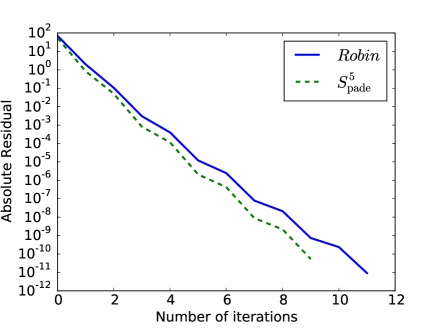
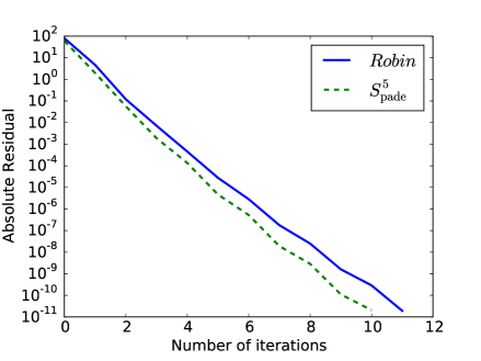
Figure 5: Convergence history of the first time step for $N=2$ (left) ,$N=32$ (right).

Table 3: Number of iterations of the first time step and total computation time in seconds, $T=0.5$, $\Delta t=0.01$, $\Delta x=1/128$, $\Delta y=1/8$.

$N$		2	4	8	16	32
	$\mathrm{Robin}^{*}$	11	11	11	11	11
Number of iterations	$S_{\mathrm{pade}}^{5}$	9	9	9	9	10
	Robin ref.	16.0
	Robin cls.	63.1	32.6	17.5	11.0	5.4
	Robin new	30.0	9.7	4.4	2.5	1.3
	$S_{\mathrm{pade}}^{5}$ ref.	22.1
	$S_{\mathrm{pade}}^{5}$ cls.	96.1	49.8	26.7	15.0	7.8
Computation time	$S_{\mathrm{pade}}^{5}$ new	38.2	14.7	6.6	3.4	1.8

• *: $p=15$.

Remark 6.3.

From the results shown in the following subsection (see Table 5 and Table 6 together), we can see clearly the different convergence rates with the two kinds of transmission conditions.

Next we make tests with the mesh $\Delta x=1/2048$ $\Delta y=1/64$. The entire domain is divided into $N=128,256,512,1024$ subdomains. We present in Figure 6 the convergence history for $N=256,1024$ and in Table 4 the numbers of iterations and the total computation time. We can see that the classical and the new algorithms are not very scalable since the number of iterations increases with the number of subdomains. However, the new algorithm takes less computation time. Besides, the number of iterations required for the transmission condition $S_{\mathrm{pade}}^{m}$ is less than the one for the Robin transmission condition. The computation times are however similar.

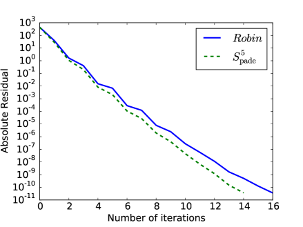
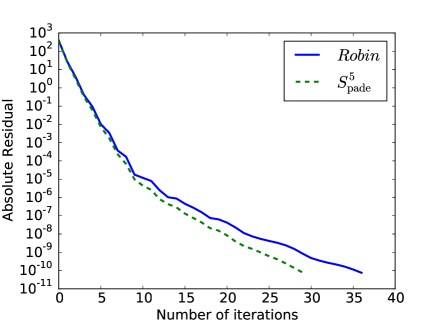
Figure 6: Convergence history of the first time step for $N=256$ (left), $N=1024$ (right).

Table 4: Number of iterations of the first time step and total computation time in seconds, $T=0.5$, $\Delta t=0.01$, $\Delta x=1/2048$, $\Delta y=1/64$.

$N$		128	256	512	1024
	$\mathrm{Robin}^{*}$	14	16	22	36
Number of iterations	$S_{\mathrm{pade}}^{5}$	12	14	19	29
	Robin cls.	250.2	143.8	92.5	101.4
	Robin new	59.1	38.1	36.2	52.3
	$S_{\mathrm{pade}}^{5}$ cls.	-	187.5	162.6	127.5
Computation time	$S_{\mathrm{pade}}^{5}$ new	-	42.7	36.2	45.0

• -: the memory is insufficient;   *: $p=10$.

6.1.3 Influence of parameters

We study in this part the influence of parameters: $m$ in the transmission condition $S_{\mathrm{pade}}^{m}$ and $p$ in the transmission condition Robin. The time step is fixed as $\Delta t=0.01$. The mesh is $\Delta x=1/128$, $\Delta y=1/8$. Three different methods are used to solve the the interface problem: fixed point method, GMRES method and BiCGStab method. Two initial vectors are considered: the zero vector and the random vector. In our tests, the algorithm initialized with the zero vector converges faster than the one with the random vector. However, in this subsection, our goal is to study the influence of parameters. As explained in [9], initialization with a zero vector to compute a smooth solution makes that the error contains only low frequencies and could therefore draw the wrong conclusions. Thus we consider both of the two initial vectors, but we have no wish to compare them.

The parameter $m$ in the transmission condition $S_{\mathrm{pade}}^{m}$. The numbers of iterations of the first time step with various $m$ are presented in Table 5. We could see that the number of iterations is not sensitive to the parameter $m$ if the GMRES method or the BiCGStab method is used on the interface problem. However, if the fixed point method is used, increasing the order of $S_{\mathrm{pade}}^{m}$ does not ensure better convergence property. The transmission condition $S_{\mathrm{pade}}^{m}$ is based on formal Padé approximation of square root operator, this approximation may deteriorate for large $m$.

Table 5: Number of iterations for different $m$, $N=32$.

	Fixed point		GMRES		BiCGStab
$m$	Zero	Random	Zero	Random	Zero	Random
3	34	124	11	30	6	17
4	26	96	10	28	6	16
5	21	79	10	27	5	15
6	18	68	9	26	5	15
7	17	61	9	25	5	14
8	18	56	9	25	5	14
9	19	52	10	25	5	14
10	21	50	10	25	5	14
15	32	46	11	26	6	15
20	43	50	12	28	6	16

The parameter $p$ in the transmission condition Robin. We present in Table 6 the numbers of iterations with various $p$ for $N=32$. From the table, we can see that the algorithm is not sensitive to $p$ if the GMRES method or the BiCGStab method is used on the interface problem, while it exists an optimal $p$ (marked with an underline) if the fixed point method is used. Besides, the Krylov methods could accelerate a lot the convergence.

Table 6: Number of iterations for different $p$, $N=32$.

	Fixed point		GMRES		BiCGStab
$p$	Zero	Random	Zero	Random	Zero	Random
$5$	57	580	11	35	6	21
$10$	34	315	11	32	6	19
$15$	32	239	11	31	6	18
$20$	35	209	11	31	6	19
$25$	40	200	11	32	6	19
$30$	46	199	11	32	6	19
$35$	52	204	12	33	6	19
$40$	59	209	12	33	6	20
$45$	65	222	12	34	6	20
$15$	32
$26$		198

In conclusion, the difference between the two transmission conditions is clear if the fixed point method is applied to the interface problem and the initial vector is the random vector (see Tables 5 and 6 together). The number of iterations for the transmission condition $S_{\mathrm{pade}}^{m}$ is less than that for the transmission condition Robin. But the difference is smaller using the Krylov methods and the zero vector as the initial vector. From the point of view of computation time, the zero vector and the GMRES method are a good choice. According to the tests in the previous subsection, the computation time for the two transmission conditions are similar.

6.2 Case of non-zero potential

The aim of this section is to compare the classical algorithm and the preconditioned algorithm in the framework of the DDS method with the fixed point method used on the interface problem. We first consider the potential $V=x^{2}+y^{2}$. Let us denote by $N_{\mathrm{nopc}}$ (resp. $N_{\mathrm{pc}}$) the number of iterations required to obtain convergence of the classical algorithm (resp. the preconditioned algorithm) and $T_{\mathrm{nopc}}$ (resp. $T_{\mathrm{pc}}$) the computation time of the classical algorithm (resp. the preconditioned algorithm).

First, we present in Figure 7 the spectral properties of $(I-\mathcal{L})$ and $P^{-1}(I-\mathcal{L})$ for $N=2,8$ subdomains. We see that the eigenvalues of $P^{-1}(I-\mathcal{L})$ are closer to $1+0i$ than those of $(I-\mathcal{L})$. The convergence history is therefore better. The Table 7 shows the number of iterations of the first time step and the total computation time to realize a complete simulation. The mesh is $\Delta x=1/128$, $\Delta y=1/8$. As mentioned before, it is possible to solve the Schrödinger equation on the entire domain with this mesh. The computation time is denoted by $T^{\mathrm{ref}}$. We can see that all algorithms are robust and the number of iterations is independent of the number of subdomains. The classical algorithm and the preconditioned algorithm are both scalable and the preconditioner allows to reduce the number of iterations and the total computation time. In addition, the times of computation $T_{\mathrm{nopc}}$, $T_{\mathrm{pc}}$ are less than the reference time $T^{\mathrm{ref}}$ if $N$ is large.

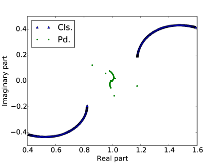
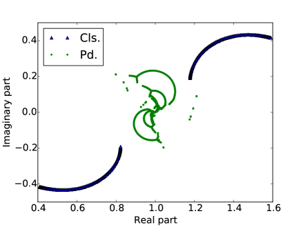
Figure 7: Eigenvalues of the classical (Cls. ) and the preconditioned (Pd.) algorithm, first time step, $\Delta t=0.01$, $\Delta x=1/128$, $\Delta y=1/8$, $N=2$ (left), $N=8$ (right).

Table 7: Number of iterations of the first time step and total computation time in seconds of the classical algorithm and the preconditioned algorithm, $T=0.5$, $\Delta t=0.01$, $\Delta x=1/128$, $\Delta y=1/8$.

$N$	2	4	8	16	32
$N_{\mathrm{nopc}}$, $m=7$	17	17	17	17	17
$N_{\mathrm{pc}}$, $m=5$	5	5	5	5	5
$T^{\mathrm{ref}}$	16.1
$T_{\mathrm{nopc}}$	142.7	75.3	40.1	23.9	12.1
$T_{\mathrm{pc}}$	91.3	43.3	22.8	13.1	7.3

Next, we consider the mesh $\Delta x=1/2048,\Delta y=1/64$. The size of $(I-\mathcal{L})$ is too large to compute all its spectral values. The convergence history and the computation time are presented in Figure 8 and Table 8. The parameters $m$ used are also presented in Table 8. We can see that the preconditioned algorithm is more robust and requires much less number of iterations. However the computation time of the two algorithms are not quite scalable since for the classical algorithm, the number of iterations increases with the number of subdomains. Concerning the preconditioned algorithm, the size of preconditioner is $(2N-2)\times N_{T}\times N_{y}$. This increases with the number of subdomains $N$. Thus, the application of preconditioner takes more computation time with bigger $N$.

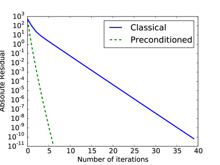
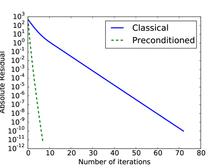
Figure 8: Convergence history of the first time step of the classical algorithm and the preconditioned algorithm, $\Delta t=0.01$, $\Delta x=1/2048$, $\Delta y=1/64$, $N=256$ (left), $N=512$ (right).

Table 8: Computation time in seconds of the classical algorithm and the preconditioned algorithm, $\Delta t=0.01,\Delta x=1/2048,\Delta y=1/64$.

$N$		256	512
Classical algorithm	$m$	8	12
	$T_{\mathrm{nopc}}$	417.9	344.9
Preconditioned algorithm	$m$	5	6
	$T_{\mathrm{pc}}$	259.9	268.7

We finish this subsection by some numerical tests for a time dependent potential $V=5(x^{2}+y^{2})(1+\cos(4\pi t))$. We get similar conclusion by the results shown in table 9.

Table 9: Number of iterations of the first time step and total computation time in seconds of the classical algorithm and the preconditioned algorithm, $T=0.5$, $\Delta t=0.01$, $\Delta x=1/128$, $\Delta y=1/8$.

$N$	2	4	8	16	32
$N_{\mathrm{nopc}}$, $p=-10$	31	31	31	31	31
$N_{\mathrm{pc}}$, $p=-10$	9	9	9	9	9
$T^{\mathrm{ref}}$	263.2
$T_{\mathrm{nopc}}$	272.6	138.5	72.4	40.5	19.5
$T_{\mathrm{pc}}$	205.6	101.4	52.2	29.4	14.8

In conclusion, the preconditioner allows to reduce significantly the number of iterations and the computation time.

7 Conclusion

We applied the SWR method and the DDS method to the two dimensional linear Schrödinger equation with general potential. We proposed a new algorithm if the potential is a constant and a preconditioned algorithm for a general linear potential, which allows to reduce the number of iterations and the computation time compared with the classical one. According to the numerical tests, the preconditioned algorithm is not sensitive to the transmission conditions (Robin, $S_{\mathrm{pade}}^{m}$) and the parameters in these conditions.

References

- [1] X. Antoine, C. Besse, and P. Klein. Absorbing Boundary Conditions for the Two-Dimensional Schrödinger Equation With an Exterior Potential Part I: Construction and a Priori Estimates. Math. Model. Methods Appl. Sci., 22(10), Oct. 2012.
- [2] X. Antoine, C. Besse, and P. Klein. Absorbing boundary conditions for the two-dimensional Schrödinger equation with an exterior potential. Part II: Discretization and numerical results. Numer. Math., 125(2):191–223, 2013.
- [3] X. Antoine, E. Lorin, and A. Bandrauk. Domain decomposition method and high-order absorbing boundary conditions for the numerical simulation of the time dependent schrödinger equation with ionization and recombination by intense electric field. J. Sci. Comput., pages 1–27, 2014.
- [4] S. Balay, M. F. Adams, J. Brown, P. Brune, K. Buschelman, V. Eijkhout, W. D. Gropp, D. Kaushik, M. G. Knepley, L. C. McInnes, K. Rupp, B. F. Smith, and H. Zhang. PETSc Users Manual. Technical Report ANL-95/11 - Revision 3.4, Argonne National Laboratory, 2013.
- [5] C. Besse and F. Xing. Schwarz waveform relaxation method for one dimensional Schrödinger equation with general potential. Preprint, arXiv: 1503.02564, 2015.
- [6] Y. Boubendir, X. Antoine, and C. Geuzaine. A quasi-optimal non-overlapping domain decomposition algorithm for the Helmholtz equation. J. Comput. Phys., 231(2):262–280, 2012.
- [7] X.-C. Cai. Multiplicative Schwarz methods for parabolic problems. SIAM J. Sci. Comput., pages 1–18, 1994.
- [8] M. J. Gander. Optimized Schwarz Methods. SIAM J. Numer. Anal., 44(2):699–731, Jan. 2006.
- [9] M. J. Gander. Schwarz methods over the course of time. Electron. Trans. Numer. Anal., 31:228–255, 2008.
- [10] M. J. Gander, L. Halpern, and F. Nataf. Optimal Schwarz waveform relaxation for the one dimensional wave equation. SIAM J. Numer. Anal., 41(5):1643–1681, 2003.
- [11] L. Halpern and J. Szeftel. Optimized and quasi-optimal Schwarz waveform relaxation for the one dimensional Schrödinger equation. Math. Model. Methods Appl. Sci., 20(12):2167–2199, Dec. 2010.
- [12] V. Martin. An optimized Schwarz waveform relaxation method for the unsteady convection diffusion equation in two dimensions. Appl. Numer. Math., 52(4):401–428, Mar. 2005.
- [13] F. Nataf and F. Rogier. Factorization of the convection-diffusion operator and the Schwarz algorithm. Math. Model. Methods Appl. Sci., 05(01):67–93, Feb. 1995.
- [14] Y. Wu, X.-C. Cai, and D. E. Keyes. Additive Schwarz methods for hyperbolic equations. Contemp. Math., 218:468–476, 1998.