DIV=calc title paragraph subsection subsubsection 0em

A parameterized approximation algorithm for the mixed and windy Capacitated Arc Routing Problem: theory and experiments

We prove that any polynomial-time $\alpha(n)$-approximation algorithm for the $n$-vertex metric asymmetric Traveling Salesperson Problem yields a polynomial-time $O(\alpha(C))$-approximation algorithm for the mixed and windy Capacitated Arc Routing Problem, where $C$ is the number of weakly connected components in the subgraph induced by the positive-demand arcs—a small number in many applications. In conjunction with known results, we obtain constant-factor approximations for $C\in O(\log n)$ and $O\bigl{(}{\log C}/{\log\log C}\bigr{)}$-approximations in general. Experiments show that our algorithm, together with several heuristic enhancements, outperforms many previous polynomial-time heuristics. Finally, since the solution quality achievable in polynomial time appears to mainly depend on $C$ and since $C=1$ in almost all benchmark instances, we propose the Ob benchmark set, simulating cities that are divided into several components by a river.

Keywords:

vehicle routing; transportation; Rural Postman; Chinese Postman; NP-hard problem; fixed-parameter algorithm; combinatorial optimization

1 Introduction

Golden and Wong [25] introduced the Capacitated Arc Routing Problem (CARP) in order to model the search for minimum-cost routes for vehicles of equal capacity that are initially located in a vehicle depot and have to serve all “customer” demands. Applications of CARP include snow plowing, waste collection, meter reading, and newspaper delivery [12]. Herein, the customer demands require that roads of a road network are served. The road network is modeled as a graph whose edges represent roads and whose vertices can be thought of as road intersections. The customer demands are modeled as positive integers assigned to edges. Moreover, each edge has a cost for traveling along it.

Problem 1.1 (Capacitated Arc Routing Problem (CARP)).

Instance: An undirected graph $G=(V,E)$, a depot vertex $v_{0}\in V$, travel costs $c\colon E\to\mathbb{N}\cup\{0\}$, edge demands $d\colon E\to\mathbb{N}\cup\{0\}$, and a vehicle capacity $Q{}$.

Task: Find a set $W{}$ of closed walks in $G$, each corresponding to the route of one vehicle and passing through the depot vertex $v_{0}$, and find a serving function $s\colon W{}\to 2^{E}$ determining for each closed walk $w\in W{}$ the subset $s(w)$ of edges served by $w$ such that

• $\sum_{w\in W{}}c(w)$ is minimized, where $c(w):=\sum_{i=1}^{\ell}c(e_{i})$ for a walk $w=(e_{1},e_{2},\dots,e_{\ell})\in E^{\ell}$,

• $\sum_{e\in s(w)}d(e)\leq Q{}$, and

• each edge $e$ with $d(e)>0$ is served by exactly one walk in $W{}$.

Note that vehicle routes may traverse each vertex or edge of the input graph multiple times. Well-known special cases of CARP are the NP-hard Rural Postman Problem (RPP) [32], where the vehicle capacity is unbounded and, hence, the goal is to find a shortest possible route for one vehicle that visits all positive-demand edges, and the polynomial-time solvable Chinese Postman Problem (CPP) [18, 19], where additionally all edges have positive demand.

1.1 Mixed and windy variants

CARP is polynomial-time constant-factor approximable [6, 31, 41]. However, as noted by van Bevern et al. [7, Challenge 5] in a recent survey on the computational complexity of arc routing problems, the polynomial-time approximability of CARP in directed, mixed, and windy graphs is open. Herein, a mixed graph may contain directed arcs in addition to undirected edges for the purpose of modeling one-way roads or the requirement of servicing a road in a specific direction or in both directions. In a windy graph, the cost for traversing an undirected edge $\{u,v\}$ in the direction from $u$ to $v$ may be different from the cost for traversing it in the opposite direction (this models sloped roads, for example). In this work, we study approximation algorithms for mixed and windy variants of CARP. To formally state these problems, we need some terminology related to mixed graphs.

Definition 1.2 (Walks in mixed and windy graphs).

A mixed graph is a triple $G=(V,E,A)$, where $V$ is a set of vertices, $E\subseteq\{\{u,v\}\mid u,v\in V\}$ is a set of (undirected) edges, $A\subseteq V\times V$ is a set of (directed) arcs (that might contain loops), and no pair of vertices has an arc and an edge between them. The head of an arc $(u,v)\in V\times V$ is $v$, its tail is $u$.

A walk in $G$ is a sequence $w=(a_{1},a_{2},\dots,a_{\ell})$ such that, for each $a_{i}=(u,v)$, $1\leq i\leq\ell$, we have $(u,v)\in A$ or $\{u,v\}\in E$, and such that the tail of $a_{i}$ is the head of $a_{i-1}$ for $1<i\leq\ell$. If $(u,v)$ occurs in $w$, then we say that $w$ traverses the arc $(u,v)\in A$ or the edge $\{u,v\}\in E$. If the tail of $a_{1}$ is the head of $a_{\ell}$, then we call $w$ a closed walk.

Denoting by $c\colon V\times V\to\mathbb{N}\cup\{0,\infty\}$ the travel cost between vertices of $G$, the cost of a walk $w=(a_{1},\dots,a_{\ell})$ is $c(w):=\sum_{i=1}^{\ell}c(a_{i})$. The cost of a set $W{}$ of walks is $c(W{}):=\sum_{w\in W{}}c(w)$.

We study approximation algorithms for the following problem.

Problem 1.3 (Mixed and windy CARP (MWCARP)).

Instance: A mixed graph $G=(V,E,A)$, a depot vertex $v_{0}\in V$, travel costs $c\colon V\times V\to\mathbb{N}\cup\{0,\infty\}$, demands $d\colon E\cup A\to\mathbb{N}\cup\{0\}$, and a vehicle capacity $Q{}$.

Task: Find a minimum-cost set $W{}$ of closed walks in $G$, each passing through the depot vertex $v_{0}$, and a serving function $s\colon W{}\to 2^{E\cup A}$ determining for each walk $w\in W{}$ the subset $s(w)$ of the edges and arcs it serves such that

• $\sum_{e\in s(w)}d(e)\leq Q{}$, and

• each edge or arc $e$ with $d(e)>0$ is served by exactly one walk in $W{}$.

For brevity, we use the term “arc” to refer to both undirected edges and directed arcs. Besides studying the approximability of MWCARP, we also consider the following special cases.

If the vehicle capacity $Q$ in MWCARP is unlimited (that is, larger than the sum of all demands) and the depot $v_{0}$ is incident to a positive-demand arc, then one obtains the mixed and windy Rural Postman Problem (MWRPP):

Problem 1.4 (Mixed and windy RPP (MWRPP)).

Instance: A mixed graph $G=(V,E,A)$ with travel costs $c\colon V\times V\to\mathbb{N}\cup\{0,\infty\}$ and a set $R\subseteq E\cup A$ of required arcs.

Task: Find a minimum-cost closed walk in $G$ traversing all arcs in $R$.

If, furthermore, $E=\emptyset$ in MWRPP, then we obtain the directed Rural Postman Problem (DRPP) and if $R=E\cup A$, then we obtain the mixed Chinese Postman Problem (MCPP).

1.2 An obstacle: approximating metric asymmetric TSP

Aiming for good approximate solutions for MWCARP, we have to be aware of the strong relation of its special case DRPP to the following variant of the Traveling Salesperson Problem (TSP):

Problem 1.5 (Metric asymmetric TSP ($\triangle$-ATSP)).

Instance: A set $V$ of vertices and travel costs $c\colon V\times V\to\mathbb{N}\cup\{0\}$ satisfying the triangle inequality $c(u,v)\leq c(u,w)+c(w,v)$ for all $u,v,w\in V$.

Task: Find a minimum-cost cycle that visits every vertex in $V$ exactly once.

Already Christofides et al. [11] observed that DRPP is a generalization of $\triangle$-ATSP. In fact, DRPP is at least as hard to approximate as $\triangle$-ATSP: Given a $\triangle$-ATSP instance, one obtains an equivalent DRPP instance by simply adding a zero-cost loop to each vertex and by adding these loops to the set $R$ of required arcs. This leads to the following observation.

Observation 1.6.

Any $\alpha(n)$-approximation for $n$-vertex DRPP yields an $\alpha(n)$-approximation for $n$-vertex $\triangle$-ATSP.

Interestingly, the constant-factor approximability of $\triangle$-ATSP is a long-standing open problem and the $O(\log n/\log\log n)$-approximation by Asadpour et al. [2] from 2010 is the first asymptotic improvement over the $O(\log n)$-approximation by Frieze et al. [24] from 1982. Thus, the constant-factor approximations for (undirected) CARP [6, 31, 41] and MCPP [37] cannot be simply carried over to MWRPP or MWCARP.

1.3 Our contributions

As discussed in Section 1.2, any $\alpha(n)$-approximation for $n$-vertex DRPP yields an $\alpha(n)$-approximation for $n$-vertex $\triangle$-ATSP. We first contribute the following theorem for the converse direction.

Theorem 1.7.

If $n$-vertex $\triangle$-ATSP is $\alpha(n)$-approximable in $t(n)$ time, then

1. $n$-vertex DRPP is $(\alpha(C)+1)$-approximable in $t(C)+O(n^{3}\log n)$ time,

2. $n$-vertex MWRPP is $(\alpha(C)+3)$-approximable in $t(C)+O(n^{3}\log n)$ time, and

3. $n$-vertex MWCARP is $(8\alpha(C+1)+27)$-approximable in $t(C+1)+O(n^{3}\log n)$ time,

where $C$ is the number of weakly connected components in the subgraph induced by the positive-demand arcs and edges.

The approximation factors in Theorem 1.7(iii) and Corollary 1.8 below are rather large. Yet in the experiments described in Section 5, the relative error of the algorithm was always below 5/4.

We prove Theorem 1.7(i–ii) in Section 3 and Theorem 1.7(iii) in Section 4. Given Theorem 1.7 and Observation 1.6, the solution quality achievable in polynomial time appears to mainly depend on the number $C$. The number $C$ is small in several applications, for example, when routing street sweepers and snow plows. Indeed, we found $C=1$ in all but one instance of the benchmark sets mval and lpr of Belenguer et al. [4] and egl-large of Brandão and Eglese [10]. This makes the following corollary particularly interesting.

Corollary 1.8.

MWCARP is 35-approximable in $O(2^{C}C^{2}+n^{3}\log n)$ time, that is, constant-factor approximable in polynomial time for $C\in O(\log n)$.

Corollary 1.8 follows from Theorem 1.7 and the exact $O(2^{n}n^{2})$-time algorithm for $n$-vertex $\triangle$-ATSP by Bellman [5] and Held and Karp [30]. It is “tight” in the sense that finding polynomial-time constant-factor approximations for MWCARP in general would, via Observation 1.6, answer a question open since 1982 and that computing optimal solutions of MWCARP is NP-hard even if $C=1$ [7].

In Section 5, we evaluate our algorithm on the mval, lpr, and egl-large benchmark sets and find that it outperforms many previous polynomial-time heuristics. Some instances are solved to optimality. Moreover, since we found that the solution quality achievable in polynomial time appears to crucially depend on the parameter $C$ and almost all of the above benchmark instances have $C=1$, we propose a method for generating benchmark instances that simulate cities separated into few components by a river, resulting in the Ob benchmark set.

1.4 Related work

Several polynomial-time heuristics for variants of CARP are known [25, 34, 4, 10] and, in particular, used for computing initial solutions for more time-consuming local search and genetic algorithms [4, 10]. Most heuristics are improved variants of three basic approaches:

Augment and merge

heuristics start out with small vehicle tours, each serving one positive-demand arc, then successively grow and merge these tours while maintaining capacity constraints [25].

Path scanning

heuristics grow vehicle tours by successively augmenting them with the “most promising” positive-demand arc [26], for example, by the arc that is closest to the previously added arc.

Route first, cluster second

approaches first construct a giant tour that visits all positive-demand arcs, which can then be split optimally into subsegments satisfying capacity constraints [3, 40].

The giant tour for the “route first, cluster second” approach can be computed heuristically [4, 10], yet when computing it using a constant-factor approximation for the undirected RPP, one can split it to obtain a constant-factor approximation for the undirected CARP [31, 41]. Notably, the “route first, cluster second” approach is the only one known to yield solutions of guaranteed quality for CARP in polynomial time. One barrier for generalizing this result to MWCARP is that already approximating MWRPP is challenging (see Section 1.2). Indeed, the only polynomial-time algorithms with guaranteed solution quality for arc routing problems in mixed graphs are for variants to which Observation 1.6 does not apply since all arcs and edges have to be served [37, 15].

Our algorithm follows the “route first, cluster second” approach: We first compute an approximate giant tour using Theorem 1.7(ii) and then, analogously to the approximation algorithms for undirected CARP [31, 41], split it to obtain Theorem 1.7(iii). However, since the analyses of the approximation factor for undirected CARP rely on symmetric distances between vertices [31, 41], our analysis is fundamentally different. Our experiments show that computing the giant tour using Theorem 1.7(ii) is beneficial compared to computing it heuristically like Belenguer et al. [4] and Brandão and Eglese [10].

Notably, the approximation factor of Theorem 1.7 depends on the number $C$ of connected components in the graph induced by positive-demand arcs. This number $C$ is small in many applications and benchmark data sets, a fact that inspired the development of exact exponential-time algorithms for RPP which are efficient when $C$ is small [21, 28, 38, 39]. Orloff [35] noticed already in 1976 that the number $C$ is a determining factor for the computational complexity of RPP. Theorem 1.7 shows that it is also a determining factor for the solution quality achievable in polynomial time.

In terms of parameterized complexity theory [17, 14], one can interpret Corollary 1.8 as a fixed-parameter constant-factor approximation algorithm [33] for MWCARP parameterized by $C$.

2 Preliminaries

Although we consider problems on mixed graphs as defined in Definition 1.2, in some of our proofs we use more general mixed multigraphs $G=(V,E,A)$ with a set $V=:V(G)$ of vertices, a multiset $E=:E(G)$ over $\{\{u,v\}\mid u,v\in V\}$ of (undirected) edges, a multiset $A=:A(G)$ over $V\times V$ of (directed) arcs that may contain self-loops, and travel costs $c\colon V\times V\to\mathbb{N}\cup\{0,\infty\}$. If $E=\emptyset$, then $G$ is a directed multigraph.

From Definition 1.2, recall the definition of walks in mixed graphs. An Euler tour for $G$ is a closed walk that traverses each arc and each edge of $G$ exactly as often as it is present in $G$. A graph is Eulerian if it allows for an Euler tour. Let $w=(a_{1},a_{2},\dots,a_{\ell})$ be a walk. The starting point of $w$ is the tail of $a_{1}$, the end point of $w$ is the head of $a_{\ell}$. A segment of $w$ is a consecutive subsequence of $w$. Two segments $w_{1}=(a_{i},\dots,a_{j})$ and $w_{2}=(a_{i^{\prime}},\dots,a_{j^{\prime}})$ of the walk $w$ are non-overlapping if $j<i^{\prime}$ or $j^{\prime}<i$. Note that two segments of $w$ might be non-overlapping yet share arcs if $w$ contains an arc several times. The distance $\text{dist}_{G}(u,v)$ from vertex $u$ to vertex $v$ of $G$ is the minimum cost of a walk in $G$ starting in $u$ and ending in $v$.

The underlying undirected (multi)graph of $G$ is obtained by replacing all directed arcs by undirected edges. Two vertices $u,v$ of $G$ are (weakly) connected if there is a walk starting in $u$ and ending in $v$ in the underlying undirected graph of $G$. A (weakly) connected component of $G$ is a maximal subgraph of $G$ in which all vertices are mutually (weakly) connected.

For a multiset $R\subseteq V\times V$ of arcs, $G[R]$ is the directed multigraph consisting of the arcs in $R$ and their incident vertices of $G$. We say that $G[R]$ is the graph induced by the arcs in $R$. For a walk $w=(a_{1},\dots,a_{\ell})$ in $G$, $G[w]$ is the directed multigraph consisting of the arcs $a_{1},\dots,a_{\ell}$ and their incident vertices, where $G[w]$ contains each arc with the multiplicity it occurs in $w$. Note that $G[R]$ and $G[w]$ might contain arcs with a higher multiplicity than $G$ and, therefore, are not necessarily sub(multi)graphs of $G$. Finally, the cost of a multiset $R$ is $c(R):=\sum_{a\in R}\mathbb{\nu}(a)c(a)$, where $\mathbb{\nu}(a)$ is the multiplicity of $a$ in $R$.

3 Rural Postman

This section presents our approximation algorithms for DRPP and MWRPP, thus proving Theorem 1.7(i) and (ii). Section 3.1 shows an algorithm for the special case of DRPP where the required arcs induce a subgraph with Eulerian connected components. Sections 3.2 and 3.3 subsequently generalize this algorithm to DRPP and MWRPP by adding to the set of required arcs an arc set of minimum weight so that the required arcs induce a graph with Eulerian connected components.

3.1 Special case: Required arcs induce Eulerian components

To turn $\alpha(n)$-approximations for $n$-vertex $\triangle$-ATSP into $(\alpha(C)+1)$-approximations for this special case of DRPP, we use LABEL:alg:eulerian-rp. The two main steps of the algorithm are illustrated in Figure 3.1: The algorithm first computes an Euler tour for each connected component of the graph $G[R]$ induced by the set $R$ of required arcs and then connects them using an approximate $\triangle$-ATSP tour on a vertex set $V_{R}$ containing (at least) one vertex of each connected component of $G[R]$.

(a) Input: Only required arcs $R$ are shown, vertices in $V_{R}$ are black.

(b) Compute Euler tours $T_{i}$ (dashed) for each connected component of $G[R]$.

(c) Add closed walk $T_{G}$ with the vertices in $V_{R}$ to get a feasible solution $T$ (dashed).

Figure 3.1: Steps of LABEL:alg:eulerian-rp to compute feasible solutions for DRPP when all connected components of $G[R]$ are Eulerian.

The following Lemma 3.1 gives a bound on the cost of the solution returned by LABEL:alg:eulerian-rp. LABEL:alg:eulerian-rp and Lemma 3.1 are more general than necessary for this special case of DRPP. In particular, we will not exploit yet that they allow $R$ to be a multiset and $V_{R}$ to contain more than one vertex of each connected component of $G[R]$. This will become relevant in Section 3.2, when we use LABEL:alg:eulerian-rp as a subprocedure to solve the general DRPP.

Input: A directed graph $G$ with travel costs $c{}$, a multiset $R$ of arcs of $G$ such that $G[R]$ consists of $C$ Eulerian connected components, and a set $V_{R}\subseteq V(G[R])$ containing at least one vertex of each connected component of $G[R]$.

1

Output: A closed walk traversing all arcs in $R$.

2

3for $i=1,\dots,C$ do

4       $v_{i}\leftarrow{}$any vertex of $V_{R}$ in component $i$ of $G[R]$;

5       $T_{i}\leftarrow{}$Euler tour of connected component $i$ of $G[R]$ starting and ending in $v_{i}$;

6

7$(V_{R},c^{\prime})\leftarrow{}$$\triangle$-ATSP instance on the vertices $V_{R}$, where $c^{\prime}(v_{i},v_{j}):=\text{dist}_{G}(v_{i},v_{j})$;

8

9$T_{V_{R}}\leftarrow\alpha(|V_{R}|)$-approximate $\triangle$-ATSP solution for $(V_{R},c^{\prime})$;

10

11$T_{G}\leftarrow{}$closed walk for $G$ obtained by replacing each arc $(v_{i},v_{j})$ on $T_{V_{R}}$ by a shortest path from $v_{i}$ to $v_{j}$ in $G$;

12

13$T\leftarrow{}$closed walk obtained by following $T_{G}$ and taking a detour $T_{i}$ whenever reaching a vertex $v_{i}$;

14

15return $T$;

16

algorithm]alg:eulerian-rp

Algorithm 3.1 Algorithm for the proof of Lemma 3.1

Lemma 3.1.

Let $G$ be a directed graph with travel costs $c{}$, let $R$ be a multiset of arcs of $G$ such that $G[R]$ consists of $C$ Eulerian connected components, let $V_{R}\subseteq V(G[R])$ be a vertex set containing at least one vertex of each connected component of $G[R]$, and let $\tilde{T}$ be any closed walk containing the vertices $V_{R}$.

If $n$-vertex $\triangle$-ATSP is $\alpha(n)$-approximable in $t(n)$ time, then LABEL:alg:eulerian-rp applied to $(G,c,R)$ and $V_{R}$ returns a closed walk of cost at most $c(R)+\alpha(|V_{R}|)\cdot c(\tilde{T})$ in $t(|V_{R}|)+O(n^{3})$ time that traverses all arcs of $R$.

Proof.

We first show that the closed walk $T$ returned by LABEL:alg:eulerian-rp visits all arcs in $R$. Since the $\triangle$-ATSP solution $T_{V_{R}}$ constructed in Algorithm 3.1 visits all vertices $V_{R}$, in particular $v_{1},\dots,v_{C}$, so does the closed walk $T_{G}$ constructed in Algorithm 3.1. Thus, for each vertex $v_{i}$, $1\leq i\leq C$, $T$ takes Euler tour $T_{i}$ through the connected component $i$ of $G[R]$ and, thus, visits all arcs in $R$.

We analyze the cost $c(T)$. The closed walk $T$ is composed of the Euler tours $T_{i}$ computed in Algorithm 3.1 and the closed walk $T_{G}$ computed in Algorithm 3.1. Hence, $c(T)=c(T_{G})+\sum_{i=1}^{C}c(T_{i})$. Since each $T_{i}$ is an Euler tour for some connected component $i$ of $G[R]$, each $T_{i}$ visits each arc of component $i$ as often as it is contained in $R$. Consequently, $\sum_{i=1}^{C}c(T_{i})=c(R)$.

It remains to analyze $c(T_{G})$. Observe first that the distances in the $\triangle$-ATSP instance $(V_{R},c^{\prime})$ correspond to shortest paths in $G$ and thus fulfill the triangle inequality. We have $c(T_{G})=c^{\prime}(T_{V_{R}})$ by construction of the $\triangle$-ATSP instance $(V_{R},c^{\prime})$ in Algorithm 3.1 and by construction of $T_{G}$ from $T_{V_{R}}$ in Algorithm 3.1. Let $\tilde{T}$ be any closed walk containing $V_{R}$ and let $T^{*}_{V_{R}}$ be an optimal solution for the $\triangle$-ATSP instance $(V_{R},c^{\prime})$. If we consider the closed walk $\tilde{T}_{V_{R}}$ that visits the vertices $V_{R}$ of the $\triangle$-ATSP instance $(V_{R},c^{\prime})$ in the same order as $\tilde{T}$, we get $c^{\prime}(T^{*}_{V_{R}})\leq c^{\prime}(\tilde{T}_{V_{R}})\leq c(\tilde{T})$. Since the closed walk $T_{V_{R}}$ computed in Algorithm 3.1 is an $\alpha(|V_{R}|)$-approximate solution to the $\triangle$-ATSP instance $(V_{R},c^{\prime})$, it finally follows that $c(T_{G})=c^{\prime}(T_{V_{R}})\leq\alpha(|V_{R}|)\cdot c^{\prime}(T^{*}_{V_{R}})\leq\alpha(|V_{R}|)\cdot c(\tilde{T})$.

Regarding the running time, observe that the instance $(V_{R},c^{\prime})$ in Algorithm 3.1 can be constructed in $O(n^{3})$ time using the Floyd-Warshall all-pair shortest path algorithm [20], which dominates all other steps of the algorithm except for, possibly, Algorithm 3.1. ∎

Lemma 3.1 proves Theorem 1.7(i) for DRPP instances $I=(G,c,R)$ when $G[R]$ consists of Eulerian connected components: Pick $V_{R}$ to contain exactly one vertex of each of the $C$ connected components of $G[R]$. Since an optimal solution $T^{*}$ for $I$ visits the vertices $V_{R}$ and satisfies $c(R)\leq c(T^{*})$, LABEL:alg:eulerian-rp yields a solution of cost at most $c(T^{*})+\alpha(C)\cdot c(T^{*})$.

3.2 Directed Rural Postman

In the previous section, we proved Theorem 1.7(i) for the special case of DRPP when $G[R]$ consists of Eulerian connected components. We now transfer this result to the general DRPP. To this end, observe that a feasible solution $T$ for a DRPP instance $(G,c,R)$ enters each vertex $v$ of $G$ as often as it leaves. Thus, if we consider the multigraph $G[T]$ that contains each arc of $G$ with same multiplicity as $T$, then $G[T]$ is a supermultigraph of $G[R]$ in which every vertex is balanced [16, 39]:

Definition 3.2 (Balance).

We denote the balance of a vertex $v$ in a graph $G$ as

$$\operatorname{balance}_{G}(v):=\operatorname{indeg}_{G}(v)-\operatorname{outdeg}_{G}(v).$$

We call a vertex $v$ balanced if $\operatorname{balance}_{G}(v)=0$.

Since $G[T]$ is a supergraph of $G[R]$ in which all vertices are balanced and since a directed connected multigraph is Eulerian if and only if all its vertices are balanced, we immediately obtain the below observation. Herein and in the following, for two (multi-)sets $X$ and $Y$, $X\uplus Y$ is the multiset obtained by adding the multiplicities of each element in $X$ and $Y$.

Observation 3.3.

Let $T$ be a feasible solution for a DRPP instance $(G,c,R)$ such that $G[R]$ has $C$ connected components and let $R^{*}$ be a minimum-cost multiset of arcs of $G$ such that every vertex in $G[R\uplus R^{*}]$ is balanced. Then, $c(R\uplus R^{*})\leq c(T)$ and $G[R\uplus R^{*}]$ consists of at most $C$ Eulerian connected components.

Input: A DRPP instance $I=(G,c,R)$ such that $G[R]$ has $C$ connected components and a set $V_{R}$ of vertices, one of each connected component of $G[R]$.

1

Output: A feasible solution for $I$.

2

3$f\leftarrow{}$minimum-cost flow for the UMCF instance $(G,\operatorname{balance}_{G[R]},c)$;

4

5foreach $a\in A(G)$ do add arc $a$ with multiplicity $f(a)$ to (initially empty) multiset $R^{*}$;

6 

7$T\leftarrow{}$closed walk computed by LABEL:alg:eulerian-rp applied to $(G,c,R\uplus R^{*})$ and $V_{R}$;

8 return $T$;

algorithm]alg:drpp

Algorithm 3.2 Algorithm for the proof of Lemma 3.5.

LABEL:alg:drpp computes an $(\alpha(C)+1)$-approximation for a DRPP instance $(G,c,R)$ by first computing a minimum-cost arc multiset $R^{*}$ such that $G[R\uplus R^{*}]$ contains only balanced vertices and then applying LABEL:alg:eulerian-rp to $(G,c,R\uplus R^{*})$. It is well known that the first step can be modeled using the Uncapacitated Minimum-Cost Flow Problem [11, 13, 16, 19, 22]:

Problem 3.4 (Uncapacitated Minimum-Cost Flow (UMCF)).

Instance: A directed graph $G=(V,A)$ with supply $s\colon V\to\mathbb{Z}$ and costs $c\colon A\to\mathbb{N}\cup\{0\}$.

Task: Find a flow $f\colon A\to\mathbb{N}\cup\{0\}$ minimizing $\sum_{a\in A}c(a)f(a)$ such that, for each $v\in V$,

$$\smashoperator[]{\sum_{(v,w)\in A}^{}}f(v,w)-\smashoperator[]{\sum_{(w,v)\in A}^{}}f(w,v) =s(v).$$ (FC)

Equation FC is known as the flow conservation constraint: For every vertex $v$ with $s(v)=0$, there are as many units of flow entering the node as leaving it. Nodes $v$ with $s(v)>0$ “produce” $s(v)$ units of flow, whereas nodes $v$ with $s(v)<0$ “consume” $s(v)$ units of flow. For our purposes, we will use $s(v):=\operatorname{balance}_{G[R]}(v)$. UMCF is solvable in $O(n^{3}\log n)$ time [1, Theorem 10.34].

Lemma 3.5.

Let $I:=(G,c,R)$ be a DRPP instance such that $G[R]$ has $C$ connected components, and let $V_{R}$ be a vertex set containing exactly one vertex of each connected component of $G[R]$. Moreover, consider two closed walks in $G$:

• Let $\tilde{T}$ be any closed walk containing the vertices $V_{R}$, and

• let $\hat{T}$ be any feasible solution for $I$.

If $n$-vertex $\triangle$-ATSP is $\alpha(n)$-approximable in $t(n)$ time, then LABEL:alg:drpp applied to $I$ and $V_{R}$ returns a feasible solution of cost at most $c(\hat{T})+\alpha(C)\cdot c(\tilde{T})$ in $t(C)+O(n^{3}\log n)$ time.

Proof.

For the sake of self-containment, we first prove that LABEL:alg:drpp in Algorithm 3.2 indeed computes a minimum-cost arc set $R^{*}$ such that all vertices in $G[R\uplus R^{*}]$ are balanced. This follows from the one-to-one correspondence between arc multisets $R^{\prime}$ such that $G[R\uplus R^{\prime}]$ has only balanced vertices and flows $f$ for the UMCF instance $I^{\prime}:=(G,\operatorname{balance}_{G[R]},c)$: Each vertex $v$ has $\operatorname{balance}_{G[R]}(v)$ more incident in-arcs than out-arcs in $G[R]$ and, thus, in order for $\operatorname{balance}_{G[R\uplus R^{\prime}]}(v)=0$ to hold, $R^{\prime}$ has to contain $\operatorname{balance}_{G[R]}(v)$ more out-arcs than in-arcs incident to $v$. Likewise, by (FC), in any feasible flow for $I^{\prime}$, there are $\operatorname{balance}_{G[R]}(v)$ more units of flow leaving $v$ than entering $v$.

Thus, from a multiset $R^{\prime}$ of arcs such that $G[R\uplus R^{\prime}]$ is balanced, we get a feasible flow $f$ for $I^{\prime}$ by setting $f(v,w)$ to the multiplicity of the arc $(v,w)$ in $R^{\prime}$. From a feasible flow $f$ for $I^{\prime}$, we get a multiset $R^{\prime}$ of arcs such that $G[R\uplus R^{\prime}]$ is balanced by adding to $R^{\prime}$ each arc $(v,w)$ with multiplicity $f(v,w)$. We conclude that the arc multiset $R^{*}$ computed in Algorithm 3.2 is a minimum-cost set such that $G[R\uplus R^{*}]$ is balanced: A set of lower cost would yield a flow cheaper than the optimum flow $f$ computed in Algorithm 3.2.

We use the optimality of $R^{*}$ to give an upper bound on the cost of the closed walk $T$ computed in Algorithm 3.2. Since $V_{R}$ contains exactly one vertex of each connected component of $G[R]$, it contains at least one vertex of each connected component of $G[R\uplus R^{*}]$. Therefore, LABEL:alg:eulerian-rp is applicable to $(G,c,R\uplus R^{*})$ and, by Lemma 3.1, yields a closed walk in $G$ traversing all arcs in $R\uplus R^{*}$ and having cost at most $c(R\uplus R^{*})+\alpha(|V_{R}|)\cdot c(\tilde{T})$. This is a feasible solution for $(G,c,R)$ and, since by Observation 3.3, we have $c(R\uplus R^{*})\leq c(\hat{T})$, it follows that this feasible solution has cost at most $c(\hat{T})+\alpha(C)\cdot c(\tilde{T}$).

Finally, the running time of LABEL:alg:drpp follows from the fact that the minimum-cost flow in Algorithm 3.2 is computable in $O(n^{3}\log n)$ time [1, Theorem 10.34] and that LABEL:alg:eulerian-rp runs in $t(C)+O(n^{3})$ time (Lemma 3.1). ∎

We may now prove Theorem 1.7(i).

Proof of Theorem 1.7(i).

Let $(G,c,R)$ be an instance of DRPP and let $V_{R}$ be a set of vertices containing exactly one vertex of each connected component of $G[R]$. An optimal solution $T^{*}$ for $I$ contains all arcs in $R$ and all vertices in $V_{R}$ and hence, by Lemma 3.5, LABEL:alg:drpp computes a feasible solution $T$ with $c(T)\leq c(T^{*})+\alpha(C)\cdot c(T^{*})$ for $I$. ∎

Before generalizing LABEL:alg:drpp to MWRPP, we point out two design choices in the algorithm that allowed us to prove an approximation factor. LABEL:alg:drpp has two steps: It first adds a minimum-weight set $R^{*}$ of required arcs so that $G[R\uplus R^{*}]$ has Eulerian connected components. Then, these connected components are connected using a cycle via LABEL:alg:eulerian-rp.

In the first step, it might be tempting to add a minimum-weight set $R^{\prime}$ of required arcs so that each connected component of $G[R]$ becomes an Eulerian connected component of $G[R\uplus R^{\prime}]$. However, this set $R^{\prime}$ might be more expensive than $R^{*}$: Multiple non-Eulerian connected components of $G[R]$ might be contained in one Eulerian connected component of $G[R\uplus R^{*}]$.

In the second step, it is crucial to connect the connected components of $G[R\uplus R^{*}]$ using a cycle. Christofides et al. [11] and Corberán et al. [13], for example, reverse the two phases of the algorithm and first join the connected components of $G[R]$ using a minimum-weight arborescence or spanning tree, respectively. This, however, may increase the imbalance of vertices and, thus, the weight of the arc set $R^{*}$ that has to be added in their second phase in order to balance the vertices of $G[R\uplus R^{*}]$.

Interestingly, the heuristic of Corberán et al. [13] aims to find a minimum-weight connecting arc set so that the resulting graph can be balanced at low extra cost and already Pearn and Wu [36] pointed out that, in context of the (undirected) RPP, reversing the steps in the algorithm of Christofides et al. [11] can be beneficial.

3.3 Mixed and windy Rural Postman

In the previous section, we presented LABEL:alg:drpp for DRPP in order to prove Theorem 1.7(i). We now generalize it to MWRPP in order to prove Theorem 1.7(ii).

To this end, we replace each undirected edge $\{u,v\}$ in an MWRPP instance by two directed arcs $(u,v)$ and $(v,u)$, where we force the undirected required edges of the MWRPP instance to be traversed in the cheaper direction:

Lemma 3.6.

Let $I:=(G,c,R)$ be an MWRPP instance and let $I^{\prime}:=(G^{\prime},c,R^{\prime})$ be the DRPP instance obtained from $I$ as follows:

• $G^{\prime}$ is obtained by replacing each edge $\{u,v\}$ of $G$ by two arcs $(u,v)$ and $(v,u)$,

• $R^{\prime}$ is obtained from $R$ by replacing each edge $\{u,v\}\in R$ by an arc $(u,v)$ if $c(u,v)\leq c(v,u)$ and by $(v,u)$ otherwise.

Then,

1. each feasible solution $T^{\prime}$ for $I^{\prime}$ is a feasible solution of the same cost for $I$ and,

2. for each feasible solution $T$ for $I$, there is a feasible solution $T^{\prime}$ for $I^{\prime}$ with $c(T^{\prime})<3c(T)$.

Proof.

Statement (i) is obvious since each required edge of $I$ is served by $T^{\prime}$ in at least one direction. Moreover, the cost functions in $I$ and $I^{\prime}$ are the same.

Towards (ii), let $T$ be a feasible solution for $I$, that is, $T$ is a closed walk that traverses all required arcs and edges of $I$. We show how to transform $T$ into a feasible solution for $I^{\prime}$. Let $(u,v)$ be an arbitrary required arc of $I^{\prime}$ that is not traversed by $T$. Then, $I$ contains a required edge $\{u,v\}$ and $T$ contains arc $(v,u)$ of $I^{\prime}$. Moreover, $c(u,v)\leq c(v,u)$. Thus, we can replace $(v,u)$ on $T$ by the sequence of arcs $(v,u),(u,v),(v,u)$. This sequence serves the required arc $(u,v)$ of $I^{\prime}$ and costs $c(v,u)+c(u,v)+c(v,u)\leq 3c(u,v)$. ∎

Using Lemma 3.6, it is easy to prove Theorem 1.7(ii).

Proof of Theorem 1.7(ii).

Given an MWRPP instance $I=(G,c,R)$, compute a DRPP instance $I^{\prime}:=(G^{\prime},c,R^{\prime})$ as described in Lemma 3.6. This can be done in linear time.

Let $V_{R}$ be a set of vertices containing exactly one vertex of each connected component of $G^{\prime}[R^{\prime}]$ and let $T^{*}$ be an optimal solution for $I$. Observe that $T^{*}$ is not necessarily a feasible solution for $I^{\prime}$, since it might serve required arcs of $I^{\prime}$ in the wrong direction. Yet $T^{*}$ is a closed walk in $G^{\prime}$ visiting all vertices of $V_{R}$. Moreover, by Lemma 3.6, $I^{\prime}$ has a feasible solution $T^{\prime}$ with $c(T^{\prime})\leq 3c(T^{*})$.

Thus, applying LABEL:alg:drpp to $I^{\prime}$ and $V_{R}$ yields a feasible solution $T$ of cost at most $c(T^{\prime})+\alpha(C)\cdot c(T^{*})\leq 3c(T^{*})+\alpha(C)\cdot c(T^{*})$ due to Lemma 3.5. Finally, $T$ is also a feasible solution for $I$ by Lemma 3.6. ∎

Remark 3.7.

If a required edge $\{u,v\}$ has $c(u,v)=c(v,u)$, then we replace it by two arcs $(u,v)$ and $(v,u)$ in the input graph $G$ and replace $\{u,v\}$ by an arbitrary one of them in the set $R$ of required arcs without influencing the approximation factor. This gives a lot of room for experimenting with heuristics that “optimally” orient undirected required edges when converting MWRPP to DRPP [34, 13]. Indeed, we will do so in Section 5.

4 Capacitated Arc Routing

We now present our approximation algorithm for MWCARP, thus proving Theorem 1.7(iii). Our algorithm follows the “route first, cluster second”-approach [3, 40, 23, 31, 41] and exploits the fact that joining all vehicle tours of a solution gives an MWRPP tour traversing all positive-demand arcs and the depot. Thus, in order to approximate MWCARP, the idea is to first compute an approximate MWRPP tour and then split it into subtours, each of which can be served by a vehicle of capacity $Q{}$. Then we close each subtour by shortest paths via the depot. We now describe our approximation algorithm for MWCARP in detail. For convenience, we use the following notation.

Definition 4.1 (Demand arc).

For a mixed graph $G=(V,A,E)$ with demand function $d\colon E\cup A\to\mathbb{N}\cup\{0\}$, we define

$$R_{d}:=\{a\in E\cup A\mid d(a)>0\}$$

to be the set of demand arcs.

We construct MWCARP solutions from what we call feasible splittings of MWRPP tours $T$.

Definition 4.2 (Feasible splitting).

For an MWCARP instance $I=(G,v_{0},c,d,Q{})$, let $T$ be a closed walk containing all arcs in $R_{d}$ and $W{}=(w_{1},\ldots,w_{\ell})$ be a tuple of segments of $T$. In the following, we abuse notation and refer by $W$ to both the tuple and the set of walks it contains.

Consider a serving function $s\colon W{}\to 2^{R_{d}}$ that assigns to each walk $w$ the set $s(w)$ of arcs in $R_{d}$ that it serves. We call $(W,s)$ a feasible splitting of $T$ if the following conditions hold:

1. the walks in $W$ are mutually non-overlapping segments of $T$,

2. when concatenating the walks in $W$ in order, we obtain a subsequence of $T$,

3. each $w_{i}\in W$ begins and ends with an arc in $s(w_{i})$,

4. $\{s(w_{i})\mid w_{i}\in W\}$ is a partition of $R_{d}$, and

5. for each $w_{i}\in W$, we have $\sum_{e\in s(w_{i})}d(e)\leq Q{}$ and, if $i<\ell$, then $\sum_{e\in s(w_{i})}d(e)+d(a)>Q{}$, where $a$ is the first arc served by $w_{i+1}$.

Constructing feasible splittings.

Given an MWCARP instance $I=(G,v_{0},c,d,Q{})$, a feasible splitting $(W,s)$ of a closed walk $T$ that traverses all arcs in $R_{d}$ can be computed in linear time using the following greedy strategy. We assume that each arc has demand at most $Q{}$ since otherwise $I$ has no feasible solution. Now, traverse $T$, successively defining subwalks $w\in W$ and the corresponding sets $s(w)$ one at a time. The traversal starts with the first arc $a\in R_{d}$ of $T$ and by creating a subwalk $w$ consisting only of $a$ and $s(w)=\{a\}$. On discovery of a still unserved arc $a\in R_{d}\setminus(\bigcup_{w^{\prime}\in W}s(w^{\prime}))$ do the following. If $\sum_{e\in s(w)}d(e)+d(a)\leq Q{}$, then add $a$ to $s(w)$ and append to $w$ the subwalk of $T$ that was traversed since discovery of the previous unserved arc in $R_{d}$. Otherwise, mark $w$ and $s(w)$ as finished, start a new tour $w\in W$ with $a$ as the first arc, set $s(w)=\{a\}$, and continue the traversal of $T$. If no such arc $a$ is found, then stop. It is not hard to verify that $(W,s)$ is indeed a feasible splitting.

Input: An MWCARP instance $I=(G,v_{0},c,d,Q{})$ such that $(v_{0},v_{0})\in R_{d}$ and such that $G[R_{d}]$ has $C$ connected components.

Output: A feasible solution for $I$.

1

/* Compute a base tour containing all demand arcs and the depot */

2

3$I^{\prime}\leftarrow{}$MWRPP instance $(G,c,R_{d})$;

4

5$T\leftarrow\beta(C)$-approximate MWRPP tour for $I^{\prime}$ starting and ending in $v_{0}$;

6

/* Split the base tour into one tour for each vehicle */

7 $(W,s)\leftarrow$ a feasible splitting of $T$;

8

9foreach $w\in W$ do

10      close $w$ by adding shortest paths from $v_{0}$ to $s$ and from $t$ to $v_{0}$ in $G$, where $s,t$ are the start and endpoints of $w$, respectively;

11      

12return $(W,s)$;

algorithm]alg:carp

Algorithm 4.1 Algorithm for the proof of Proposition 4.4.

The algorithm.

LABEL:alg:carp constructs an MWCARP solution from an approximate MWRPP solution $T$ containing all demand arcs and the depot $v_{0}$. In order to ensure that $T$ contains $v_{0}$, LABEL:alg:carp assumes that the input graph has a demand loop $(v_{0},v_{0})$: If this loop is not present, we can add it with zero cost. Note that, while this does not change the cost of an optimal solution, it might increase the number of connected components in the subgraph induced by demand arcs by one. To compute an MWCARP solution from $T$, LABEL:alg:carp first computes a feasible splitting $(W,s)$ of $T$. To each walk $w_{i}\in W$, it then adds a shortest path from the end of $w_{i}$ to the start of $w_{i}$ via the depot. It is not hard to check that LABEL:alg:carp indeed outputs a feasible solution by using the properties of feasible splittings and the fact that $T$ contains all demand arcs.

Remark 4.3.

Instead of computing a feasible splitting of $T$ greedily, LABEL:alg:carp could compute a splitting of $T$ into pairwise non-overlapping segments that provably minimizes the cost of the resulting MWCARP solution [40, 4, 41, 31]. Indeed, we will do so in our experiments in Section 5. For the analysis of the approximation factor, however, the greedy splitting is sufficient and more handy, since the analysis can exploit that two consecutive segments of a feasible splitting serve more than $Q$ units of demand (excluding, possibly, the last segment).

The remainder of this section is devoted to the analysis of the solution cost, thus proving the following proposition, which, together with Theorem 1.7(ii), yields Theorem 1.7(iii).

Proposition 4.4.

Let $I=(G,v_{0},c,d,Q{})$ be an MWCARP instance and let $I^{\prime}$ be the instance obtained from $I$ by adding a zero-cost demand arc $(v_{0},v_{0})$ if it is not present.

If MWRPP is $\beta(C)$-approximable in $t(n)$ time, then LABEL:alg:carp applied to $I^{\prime}$ computes a $(8\beta(C+1)+3)$-approximation for $I$ in $t(C+1)+O(n^{3})$ time. Herein, $C$ is the number of connected components in $G[R_{d}]$.

The following lemma follows from the fact that the concatenation of all vehicle tours in any MWCARP solution yields an MWRPP tour containing all demand arcs and the depot.

Lemma 4.5.

Let $I=(G,v_{0},c,d,Q{})$ be an MWCARP instance with $(v_{0},v_{0})\in R_{d}$ and an optimal solution $(W^{*},s^{*})$. The closed walk $T$ and its feasible splitting $(W,s)$ computed in Algorithms 4.1 and 4.1 of LABEL:alg:carp satisfy $c(W)\leq c(T)\leq\beta(C)c(W^{*})$, where $C$ is the number of connected components in $G[R_{d}]$.

Proof.

Consider an optimal solution $(W^{*},s^{*})$ to $I$. The closed walks in $W^{*}$ visit all arcs in $R_{d}$. Concatenating them to a closed walk $T^{*}$ gives a feasible solution for the MWRPP instance $I^{\prime}=(G,c,R_{d})$ in Algorithm 4.1 of LABEL:alg:carp. Moreover, $c(T^{*})=c(W^{*})$. Thus, we have $c(T)\leq\beta(C)c(T^{*})$ in Algorithm 4.1. Moreover, by Definition 4.2(i), one has $c(W)\leq c(T)$. This finally implies $c(W)\leq c(T)\leq\beta(C)c(T^{*})=\beta(C)c(W^{*})$ in Algorithm 4.1. ∎

For each $w_{i}\in W$, it remains to analyze the length of the shortest paths from $v_{0}$ to $w_{i}$ and from $w_{i}$ to $v_{0}$ added in Algorithm 4.1 of LABEL:alg:carp. We bound their lengths in the lengths of an auxiliary walk $A(w_{i})$ from $v_{0}$ to $w_{i}$ and of an auxiliary walk $Z(w_{i})$ from $w_{i}$ to $v_{0}$. The auxiliary walks $A(w_{i})$ and $Z(w_{i})$ consist of arcs of $W$, whose total cost is bounded by Lemma 4.5, and of arcs of an optimal solution $(W^{*},s^{*})$. We show that, in total, the walks $A(w_{i})$ and $Z(w_{i})$ for all $w_{i}\in W$ use each subwalk of $W$ and $W^{*}$ at most a constant number of times. To this end, we group the walks in $W$ into consecutive pairs, for each of which we will be able to charge the cost of the auxiliary walks to a distinct vehicle tour of the optimal solution.

Definition 4.6 (Consecutive pairing).

For a feasible splitting $(W,s)$ with $W=(w_{1},\dots,w_{\ell})$, we call

$$W^{2}{}:=\{(w_{2i-1},w_{2i})\mid i\in\{1,\ldots,\lfloor{\ell}/{2}\rfloor\}\}$$

a consecutive pairing.

We can now show, by applying Hall’s theorem [29], that each pair traverses an arc from a distinct tour of an optimal solution.

Lemma 4.7.

Let $I=(G,v_{0},c,d,Q{})$ be an MWCARP instance with an optimal solution $(W^{*},s^{*})$ and let $W^{2}{}$ be a consecutive pairing of some feasible splitting $(W,s)$. Then, there is an injective map $\phi\colon W^{2}{}\to W^{*},(w_{i},w_{i+1})\mapsto w^{*}$ such that $(s(w_{i})\cup s(w_{i+1}))\cap s^{*}(w^{*})\neq\emptyset$.

Proof.

Define an undirected bipartite graph $B$ with the partite sets $W^{2}{}$ and $W^{*}$. A pair $(w_{i},w_{i+1})\in W^{2}{}$ and a closed walk $w^{*}\in W^{*}$ are adjacent in $B$ if $(s(w_{i})\cup s(w_{i+1}))\cap s^{*}(w^{*})\neq\emptyset$. We prove that $B$ allows for a matching that matches each vertex of $W^{2}{}$ to some vertex in $W^{*}$. To this end, by Hall’s theorem [29], it suffices to prove that, for each subset $S\subseteq W^{2}{}$, it holds that $|N_{B}(S)|\geq|S|$, where $N_{B}(S):=\bigcup_{v\in S}N_{B}(v)$ and $N_{B}(v)$ is the set of neighbors of a vertex $v$ in $B$. Observe that, by Definition 4.2(v) of feasible splittings, for each pair $(w_{i},w_{i+1})\in W^{2}{}$, we have $d(s(w_{i})\cup s(w_{i+1}))\geq Q{}$. Since the pairs serve pairwise disjoint sets of demand arcs by Definition 4.2(iv), the pairs in $S$ serve a total demand of at least $Q{}\cdot|S|$ in the closed walks $N_{B}(S)\subseteq W^{*}$. Since each closed walk in $N_{B}(S)$ serves demand at most $Q{}$, the set $N_{B}(S)$ is at least as large as $S$, as required. ∎

In the following, we fix an arbitrary arc in $(s(w_{i})\cup s(w_{i+1}))\cap s^{*}(w^{*})$ for each pair $(w_{i},w_{i+1})\in W^{2}{}$ and call it the pivot arc of $(w_{i},w_{i+1})$. Informally, the auxiliary walks $A(w_{i})$, $Z(w_{i})$ mentioned before are constructed as follows for each walk $w_{i}$. To get from the endpoint of $w_{i}$ to $v_{0}$, walk along the closed walk $T$ until traversing the first pivot arc $a$, then from the head of $a$ to $v_{0}$ follow the tour of $W^{*}$ containing $a$. To get from $v_{0}$ to $w_{i}$, take the symmetric approach: walk backwards on $T$ from the start point of $w_{i}$ until traversing a pivot arc $a$ and then follow the tour of $W^{*}$ containing $a$. The formal definition of the auxiliary walks $A(w)$ and $Z(w)$ is given below and illustrated in Figure 4.1.

Figure 4.1: Illustration of Definition 4.8. Dotted lines are ancillary lines. Thin arrows are walks. The braces along the bottom show a consecutive pairing of walks $w_{i-1},\dots,w_{i+2}$. Bold arcs are pivot arcs. Here, $p(i)$ is exactly the pair that contains $w_{i}$ and $q(i)$ is the next pair.

Definition 4.8 (Auxiliary walks).

Let $I=(G,v_{0},c,d,Q{})$ be an MWCARP instance, $(W^{*},s^{*})$ be an optimal solution, and $W^{2}{}$ be a consecutive pairing of some feasible splitting $(W,s)$ of a closed walk $T$ containing all arcs $R_{d}$ and $v_{0}$, where $W{}=(w_{1},\ldots,w_{\ell})$.

Let $\phi\colon W^{2}{}\to W^{*}$ be an injective map as in Lemma 4.7 and, for each pair $(w_{i},w_{i+1})\in W^{2}$, let

• be a subwalk of $\phi(w_{i},w_{i+1})$ from $v_{0}$ to the tail of the pivot arc of $(w_{i},w_{i+1})$,

• be a subwalk of $\phi(w_{i},w_{i+1})$ from the head of the pivot arc of $(w_{i},w_{i+1})$ to $v_{0}$.

For each walk $w_{i}\in W$ with $i\geq 3$ (that is, $w_{i}$ is not in the first pair of $W^{2}{}$), let

• be the index of the pair whose pivot arc is traversed first when walking $T$ backwards starting from the starting point of $w_{i}$,

• be the subwalk of $T$ starting at the end point of $A^{*}(w_{2p(i){}-1},w_{2p(i){}})$ and ending at the start point of $w_{i}$, and

• be the walk from $v_{0}$ to the start point of $w_{i}$ following first $A^{*}(w_{2p(i){}-1},w_{2p(i){}})$ and then $A^{\prime}(w_{i})$.

For each walk $w_{i}\in W$ with $i\leq\ell-3$ (that is, $w_{i}$ is not in the last pair of $W^{2}{}$, where $w_{\ell}$ might not be in any pair if $\ell$ is odd), let

• be the index of the pair whose pivot arc is traversed first when following $T$ starting from the end point of $w_{i}$,

• be the subwalk of $T$ starting at the end point of $w_{i}$ and ending at the start point of $Z^{*}(w_{2q(i){}-1},w_{2q(i){}})$, and

• be the walk from the end point of $w_{i}$ to $v_{0}$ following first $Z^{\prime}(w_{i})$ and then $Z^{*}(w_{2q(i){}-1},w_{2q(i){}})$.

We are now ready to prove Proposition 4.4, which also concludes our proof of Theorem 1.7.

Figure 4.2: Illustration of the situation in which a maximum number of five different walks in $W$ traverse the same pivot arc (the bold arc of $w_{i}$) in their respective auxiliary walks.

Proof of Proposition 4.4.

Let $I=(G,v_{0},c,d,Q{})$ be an MWRPP instance and $(W^{*},s^{*})$ be an optimal solution. If there is no demand arc $(v_{0},v_{0})$ in $I$, then we add it with zero cost in order to make LABEL:alg:carp applicable. This clearly does not change the cost of an optimal solution but may increase the number of connected components of $G[R_{d}]$ to $C+1$.

In Algorithms 4.1 and 4.1, LABEL:alg:carp computes a tour $T$ and its feasible splitting $(W,s)$, which works in $t(C+1)+O(n^{3})$ time by Theorem 1.7(ii). Denote $W=(w_{1},\dots,w_{\ell})$. The solution returned by LABEL:alg:carp consists, for each $1\leq i\leq\ell$, of a tour starting in $v_{0}$, following a shortest path to the starting point of $w_{i}$, then $w_{i}$, and a shortest path back to $v_{0}$.

For $i\geq 3$, the shortest path from $v_{0}$ to the starting point of $w_{i}$ has length at most $c(A(w_{i}))$. For $i\leq\ell-3$, the shortest path from the end point of $w_{i}$ to $v_{0}$ has length at most $c(Z(w_{i}))$. This amounts to $\sum_{i=3}^{\ell}c(A(w_{i}))+\sum_{i=1}^{\ell-3}c(Z(w_{i}))$. To bound the costs of the shortest paths attached to $w_{i}$ for $i\in\{1,2,\ell-2,\ell-1,\ell\}$, observe the following. For each $i\in\{1,2\}$, the shortest paths from $v_{0}$ to the start point of $w_{i}$ and from the end point of $w_{\ell-i}$ to $v_{0}$ together have length at most $c(T)$. The shortest path from the end point of $w_{\ell}$ to $v_{0}$ has length at most $c(T)-c(W{})$. Thus, the solution returned by LABEL:alg:carp has cost at most

$$\sum_{i=1}^{\ell}c(w_{i})+\sum_{i=3}^{\ell}c(A(w_{i}))+\sum_{i=1}^{\ell-3}c(Z(w_{i}))+3c(T)-c(W{})$$

$$={} \sum_{i=3}^{\ell}c(A(w_{i}))+\sum_{i=1}^{\ell-3}c(Z(w_{i}))+3c(T)$$

$$={} 3c(T)+{}$$

$$+\sum_{i=3}^{\ell}c(A^{*}(w_{2p(i){}-1},w_{2p(i){}}))+\sum_{i=1}^{\ell-3}c(Z^{*}(w_{2q(i){}-1},w_{2q(i){}}))+{}$$ (S1)

$$+\sum_{i=3}^{\ell}c(A^{\prime}(w_{i}))+\sum_{i=1}^{\ell-3}c(Z^{\prime}(w_{i})).$$ (S2)

Observe that, for a fixed $i$, one has $p(i)=p(j)$ only for $j\leq i+2$ and $q(i)=q(j)$ only for $j\geq i-2$. Moreover, by Lemma 4.7 and Definition 4.8, if $p(i)\neq p(j)$, then $A^{*}(w_{2p(i)-1},w_{2p(i)})$ and $A^{*}(w_{2p(j)-1},w_{2p(j)})$ are subwalks of distinct walks of $W^{*}$. Similarly, $Z^{*}(w_{2q(i)-1},w_{2q(i)})$ and $Z^{*}(w_{2q(j)-1},w_{2q(j)})$ are subwalks of distinct walks of $W^{*}$ if $q(i)\neq q(j)$. Hence, sum (S1) counts each arc of $W^{*}$ at most three times and is therefore bounded from above by $3c(W^{*})$.

Now, for a walk $w_{i}$, let $\mathcal{A}_{i}$ be the set of walks $w_{j}$ such that any arc $a$ of $w_{i}$ is contained in $A^{\prime}(w_{j})$ and let $\mathcal{Z}_{i}$ be the set of walks such that any arc $a$ of $w_{i}$ is contained in $Z^{\prime}(w_{j})$. Observe that $A^{\prime}(w_{j})$ and $Z^{\prime}(w_{j})$ cannot completely contain two walks of the same pair of the consecutive pairing $W^{2}{}$ of $W$ since, by Lemma 4.7, each pair has a pivot arc and $A^{\prime}(w_{j})$ and $Z^{\prime}(w_{j})$ both stop after traversing a pivot arc. Hence, the walks in $\mathcal{A}_{i}\cup\mathcal{Z}_{i}$ can be from at most three pairs of $W^{2}{}$: the pair containing $w_{i}$ and the two neighboring pairs. Finally, observe that $w_{i}$ itself is not contained in $\mathcal{A}_{i}\cup\mathcal{Z}_{i}$. Thus, $\mathcal{A}_{i}\cup\mathcal{Z}_{i}$ contains at most five walks (Figure 4.2 shows a worst-case example). Therefore, sum (S2) counts every arc of $W{}$ at most five times and is bounded from above by $5c(W{})$.

Thus, LABEL:alg:carp returns a solution of cost $3c(T)+5c(W{})+3c(W^{*})$ which, by Lemma 4.5, is at most $8c(T)+3c(W^{*})\leq 8\beta(C+1)c(W^{*})+3c(W^{*})\leq(8\beta(C+1)+3)c(W^{*})$. ∎

5 Experiments

Our approximation algorithm for MWCARP is one of many “route first, cluster second”-approaches, which was first applied to CARP by Ulusoy [40] and led to constant-factor approximations for the undirected CARP [41, 31]. Notably, Belenguer et al. [4] implemented Ulusoy’s heuristic [40] for the mixed CARP by computing the base tour using path scanning heuristics. Our experimental evaluation will show that Ulusoy’s heuristic can be substantially improved by computing the base tour using our Theorem 1.7(ii).

For the evaluation, we use the mval and lpr benchmark sets of Belenguer et al. [4] for the mixed (but non-windy) CARP and the egl-large benchmark set of Brandão and Eglese [10] for the (undirected) CARP. We chose these benchmark sets because relatively good lower bounds to compare with are known [27, 9]. Moreover, the egl-large set is of particular interest since it contains large instances derived from real road networks and the mval and lpr sets are of particular interest since Belenguer et al. [4] used them to evaluate their variant of Ulusoy’s heuristic [40], which is very similar to our algorithm.

In the following, Section 5.1 describes some heuristic enhancements of our algorithm, Section 5.2 interprets our experimental results, and Section 5.3 describes an approach to transform instances of existing benchmark sets into instances whose positive-demand arcs induce a moderate number of connected components.

5.1 Implementation details

Since our main goal is evaluating the solution quality rather than the running time of our algorithm, we sacrificed speed for simplicity and implemented it in Python. Thus, the running time of our implementation is not competitive to the implementations by Belenguer et al. [4] and Brandão and Eglese [10]. However, it is clear that a careful implementation of our algorithm in C++ will yield competitive running times: The most expensive steps of our algorithm are the Floyd-Warshall all-pair shortest path algorithm [20], which is also used by Belenguer et al. [4] and Brandão and Eglese [10], and the computation of an uncapacitated minimum-cost flow, algorithms for which are contained in highly optimized C++ libraries like LEMON.

In the following, we describe heuristic improvements over the algorithms presented in Sections 3 and 4, which were described there so as to conveniently prove upper bounds rather than focusing on good solutions.

5.1.1 Joining connected components

We observed that, in all but one instance of the egl-large, lpr, and mval benchmark sets, the set of positive-demand arcs induce only one connected component. Therefore, connecting them is usually not necessary and the call to LABEL:alg:eulerian-rp in LABEL:alg:drpp can be skipped completely. If not, then, contrary to the description of LABEL:alg:eulerian-rp, we do not arbitrarily select one vertex from each connected component and join them using an approximate $\triangle$-ATSP tour as in LABEL:alg:eulerian-rp or using an optimal $\triangle$-ATSP tour as for Corollary 1.8.

Instead, using brute force, we try all possibilities of choosing one vertex from each connected component and connecting them using a cycle and choose the cheapest variant. If the positive-demand arcs induce $C$ connected components, then this takes $O(n^{C}\cdot C!+n^{3})$ time in an $n$-vertex graph. That is, for $C\leq 3$, implementing LABEL:alg:eulerian-rp in this way does not increase its asymptotic time complexity.

5.1.2 Choosing service direction

The instances in the egl-large, lpr, and mval benchmark sets are not windy. Thus, as pointed out in Remark 3.7, when computing the MWRPP base tour, we are free to choose whether to replace a required undirected edge $\{u,v\}$ by a required arc $(u,v)$ or a required arc $(v,u)$ (and adding the opposite non-required arc) without increasing the approximation factor in Theorem 1.7(ii).

We thus implemented several heuristics for choosing what we call the service direction of the undirected edge $\{u,v\}$. Some of these heuristics choose the service direction independently for each undirected edge, similarly to Corberán et al. [13], others choose it for whole undirected paths and cycles, similarly to Mourão and Amado [34].

We now describe these heuristics in detail. To this end, let $G$ denote our input graph and $R$ be the set of required arcs.

• assigns one of the two possible service directions to each undirected edge uniformly at random.

• replaces each undirected edge $\{u,v\}\in R$ by an arc $(u,v)\in R$ if $\operatorname{balance}_{G[R]}(v)<\operatorname{balance}_{G[R]}(u)$, by an arc $(v,u)\in R$ if $\operatorname{balance}_{G[R]}(v)>\operatorname{balance}_{G[R]}(u)$, and chooses a random service direction otherwise.

• randomly chooses one endpoint $v$ of each undirected edge $\{u,v\}\in R$ and replaces it by an arc $(u,v)\in R$ if $\operatorname{balance}_{G[R]}(v)<0$ and by $(v,u)\in R$ otherwise.

Herein, “EO” is for “edge orientation”. The “R” in parentheses is for “random”, the “P” for “pair” (since it levels the balances of pairs of vertices), and the “S” is for “single” (since it minimizes $|\operatorname{balance}(v)|$ of a single random endpoint $v$ of the edge).

In addition, we experiment with three heuristics that do not orient independent edges but long undirected paths. Herein, the aim is that a vehicle will be able to serve all arcs resulting from such a path in one run.

First, the heuristics repeatedly search for undirected cycles in $G[R]$ and replace them by directed cycles in $R$. When no undirected cycle is left, then the undirected edges of $G[R]$ form a forest. The heuristics then repeatedly search for a longest undirected path in $G[R]$ and choose its service direction as follows.

• assigns the service direction randomly.

• assigns the service direction by leveling the balance of the endpoints of the path, analogously to EO(P).

• assigns the service direction so as to minimize $|\operatorname{balance}(v)|$ for a random endpoint $v$ of the path, analogously to EO(S).

Generally, we observed that these heuristics first find three or four long paths with lengths from 5 up to 15. Then, the length of the found paths quickly decreases: In most instances, at least half of all found paths have length one, at least 3/4 of all found paths have length at most two.

We now present experimental results for each of these six heuristics.

5.1.3 Tour splitting

As pointed out in Remark 4.3, the MWRPP base tour initially computed in LABEL:alg:carp can be split into pairwise non-overlapping subsequences so as to minimize the total cost of the resulting vehicle tours. To this end, we apply an approach of Beasley [3] and Ulusoy [40], which by now can be considered folklore [4, 41, 31] and works as follows.

Denote the positive-demand arcs on the MWRPP base tour as a sequence $a_{1},\dots,a_{\ell}$. To compute the optimal splitting, we create an auxiliary graph with the vertices $1,\dots,\ell+1$. Between each pair $(i,j)$ of vertices, there is an edge whose weight is the cost for serving all arcs $a_{i},a_{i+1},\dots,a_{j-1}$ in this order using one vehicle. That is, its cost is $\infty$ if the demands of the arcs in this segment exceed the vehicle capacity $Q$ and otherwise it is the cost for going from the depot $v_{0}$ to the tail of $a_{i}$, serving arcs $a_{i}$ to $a_{j-1}$, and returning from the head of $a_{j-1}$ to the depot $v$. Then, a shortest path from vertex $1$ to $\ell+1$ in this auxiliary graph gives an optimal splitting of the MWRPP base tour into mutually non-overlapping subsequences.

Additionally, we implemented a trick of Belenguer et al. [4] that takes into account that a vehicle may serve a segment $a_{i},\dots,a_{k},a_{k+1}\dots,a_{j-1}$ by going to the tail of $a_{k+1}$, serving arcs $a_{k+1}$ to $a_{j-1}$, going from the head of $a_{j-1}$ to the tail of $a_{i}$, serving arcs $a_{i}$ to $a_{k}$, and finally returning from the head of $a_{k}$ to the depot $v_{0}$. Our implementation tries all such $k$ and assigns the cheapest resulting cost to the edge between the pair $(i,j)$ of vertices in the auxiliary graph.

Of course one could compute the optimal order for serving the arcs of a segment $a_{i},\dots,a_{j-1}$ from the depot $v_{0}$, but this would again be the NP-hard DRPP.

5.2 Experimental results

Our experimental results for the lpr, mval, and egl-large instances are presented in Tables 5.1 and 5.2. We grouped the results for the lpr and mval instances into one table and subsection since our conclusions about them are very similar. We explain and interpret the tables in the following.

Table 5.1: Known results [4, 27] and our results for the lpr and mval instances. See Section 5.2.1 for a description of the table. The best polynomial-time computed upper bound is written in boldface, the second best is underlined, names of instances solved optimally by our algorithms are also written in boldface.

	Known results					Our results
Instance	LB	UB	PSRC	IM	IURL	EO(R)	EO(P)	EO(S)	PO(R)	PO(P)	PO(S)
lpr-a-01	13 484	13 484	13 600	13 597	13 537	13 484	13 484	13 484	13 484	13 484	13 484
lpr-a-02	28 052	28 052	29 094	28 377	28 586	28 225	28 381	28 356	28 239	28 381	28 356
lpr-a-03	76 115	76 155	79 083	77 331	78 151	77 019	76 783	76 964	76 951	76 783	76 820
lpr-a-04	126 946	127 352	133 055	128 566	131 884	130 470	130 137	130 255	130 198	130 171	130 186
lpr-a-05	202 736	205 499	215 153	207 597	212 167	210 328	209 980	210 265	210 235	210 139	210 344
lpr-b-01	14 835	14 835	15 047	14 918	14 868	14 869	14 869	14 835	14 835	14 835	14 835
lpr-b-02	28 654	28 654	29 522	29 285	28 947	28 749	28 689	28 689	28 757	28 790	28 727
lpr-b-03	77 859	77 878	80 017	80 591	79 910	78 428	78 745	78 853	78 645	78 810	78 743
lpr-b-04	126 932	127 454	133 954	129 449	132 241	130 024	130 024	130 024	130 076	130 024	130 024
lpr-b-05	209 791	211 771	223 473	215 883	219 702	217 024	216 769	216 459	217 079	216 639	216 659
lpr-c-01	18 639	18 639	18 897	18 744	18 706	18 943	18 695	18 732	18 708	18 752	18 752
lpr-c-02	36 339	36 339	36 929	36 485	36 763	37 177	36 649	36 856	36 723	36 711	36 662
lpr-c-03	111 117	111 632	115 763	112 462	114 539	115 399	114 438	114 888	114 336	114 335	114 290
lpr-c-04	168 441	169 254	174 416	171 823	173 161	174 088	172 089	172 902	172 637	172 172	172 365
lpr-c-05	257 890	259 937	268 368	262 089	266 058	266 637	263 989	264 947	264 911	264 263	264 665
Instance	LB	UB	PSRC	IM	IURL	EO(R)	EO(P)	EO(S)	PO(R)	PO(P)	PO(S)
mval1A	230	230	243	243	231	245	230	238	234	239	234
mval1B	261	261	314	276	292	298	285	285	307	307	307
mval1C	309	315	427	352	357	367	362	362	367	372	370
mval2A	324	324	409	360	374	397	353	324	369	369	368
mval2B	395	395	471	407	434	431	424	424	424	424	424
mval2C	521	526	644	560	601	621	622	592	600	624	594
mval3A	115	115	133	119	128	131	129	125	122	121	121
mval3B	142	142	162	163	150	151	148	151	149	147	147
mval3C	166	166	191	174	192	194	190	189	194	200	200
mval4A	580	580	699	653	684	648	622	645	651	647	647
mval4B	650	650	775	693	737	709	687	709	690	674	682
mval4C	630	630	828	702	740	750	721	736	714	722	722
mval4D	746	770	1015	810	905	875	871	852	872	879	870
mval5A	597	597	733	686	683	672	619	652	614	649	644
mval5B	613	613	718	677	677	687	662	685	653	653	654
mval5C	697	697	809	743	811	788	773	778	783	804	783
mval5D	719	739	883	821	855	859	840	854	845	840	836
mval6A	326	326	392	370	367	348	347	348	344	351	350
mval6B	317	317	406	346	354	345	331	354	351	343	347
mval6C	365	371	526	402	444	455	435	435	461	454	454
mval7A	364	364	439	381	390	428	386	411	404	398	398
mval7B	412	412	507	470	491	474	435	463	460	460	454
mval7C	424	426	578	451	504	507	474	483	489	482	482
mval8A	581	581	666	639	651	648	635	635	639	627	641
mval8B	531	531	619	568	611	616	582	592	596	598	600
mval8C	617	638	842	718	762	799	737	729	776	764	779
mval9A	458	458	529	500	514	503	486	493	496	490	498
mval9B	453	453	552	534	502	518	504	503	503	523	506
mval9C	428	429	529	479	498	509	468	488	485	479	474
mval9D	514	520	695	575	622	627	603	610	612	613	608
mval10A	634	634	735	710	705	669	663	661	667	658	659
mval10B	661	661	753	717	714	708	687	693	703	703	698
mval10C	623	623	751	680	714	709	689	697	698	695	687
mval10D	643	649	847	706	760	778	739	763	775	743	722

Table 5.2: Known results [10, 9] and our results for the egl-large instances. See Section 5.2.2 for a description of the table. The best polynomial-time computed upper bound is written in boldface.

	Known results			Our results
Instance	LB	UB	PS	EO(R)	EO(P)	EO(S)	PO(R)	PO(P)	PO(S)
egl-g1-A	976 907	1 049 708	1 318 092	1 258 206	1 181 928	1 209 108	1 153 029	1 158 233	1 141 457
egl-g1-B	1 093 884	1 140 692	1 483 179	1 367 979	1 306 521	1 328 250	1 293 095	1 308 350	1 297 606
egl-g1-C	1 212 151	1 282 270	1 584 177	1 523 183	1 456 305	1 463 009	1 432 281	1 424 722	1 430 841
egl-g1-D	1 341 918	1 420 126	1 744 159	1 684 343	1 609 822	1 609 537	1 586 294	1 601 588	1 580 634
egl-g1-E	1 482 176	1 583 133	1 841 023	1 829 244	1 769 977	1 780 089	1 716 612	1 748 308	1 755 700
egl-g2-A	1 069 536	1 129 229	1 416 720	1 372 177	1 276 871	1 304 618	1 263 263	1 249 293	1 255 120
egl-g2-B	1 185 221	1 255 907	1 559 464	1 517 245	1 410 385	1 449 553	1 398 162	1 405 916	1 404 533
egl-g2-C	1 311 339	1 418 145	1 704 234	1 661 596	1 594 147	1 597 266	1 538 036	1 532 913	1 544 214
egl-g2-D	1 446 680	1 516 103	1 918 757	1 812 309	1 728 840	1 741 351	1 695 333	1 694 448	1 704 080
egl-g2-E	1 581 459	1 701 681	1 998 355	1 962 802	1 883 953	1 908 339	1 851 436	1 861 134	1 861 469

5.2.1 Results for the lpr and mval instances

Table 5.1 presents known results and our results for the lpr and mval instances. Each column for our results was obtained by running our algorithm with the corresponding service direction heuristic described in Section 5.1.2 on each instance 20 times and reporting the best result. The number 20 has been chosen so that our results are comparable with those of Belenguer et al. [4], who used the same number of runs for their path scanning heuristic (column PSRC) and their “route first, cluster second” heuristic (column IURL), which computes the base tour using a path scanning heuristic and then splits it using all tricks described in Section 5.1.3. Columns LB and UB report the best lower and upper bounds computed by Belenguer et al. [4] and Gouveia et al. [27] (usually not using polynomial-time algorithms). Finally, column IM shows the result that Belenguer et al. [4] obtained using an improved variant of the “augment and merge” heuristic due to Golden and Wong [25].

Table 5.1 shows that our algorithm with the EO(S) service direction heuristic solved three instances optimally, which other polynomial-time heuristics did not. The EO(P) heuristic solved one instance optimally, which also other polynomial-time heuristics did not. Moreover, whenever no variant of our algorithm finds the best result, then some variant yields the second best. It is outperformed only by IM in 26 out of 49 instances and by IURL in only one instance. Apparently, our algorithm outperforms PSRC and IURL. Notably, IURL differs from our algorithm only in computing the base tour heuristically instead of using our Theorem 1.7(ii). Thus, “route first, cluster second” heuristics seem to benefit from computing the base tour using our MWRPP approximation algorithm.

Remarkably, when our algorithm yields the best result using one of the service direction heuristics described in Section 5.1.2, then usually other service direction heuristics also find the best or at least the second best solution. Thus, the choice of the service direction heuristic does not play a strong role. Indeed, we also experimented with repeating our algorithm 20 times on each instance, each time choosing the service direction heuristic randomly. The results come close to choosing the best heuristic for each instance.

5.2.2 Results for the egl-large instances

Table 5.2 reports known results and our results for the egl-large benchmark set. Again, each column for our results was obtained by running our algorithm with the corresponding service direction heuristic described in Section 5.1.2 on each instance 20 times. The column LB reports lower bounds by Bode and Irnich [9], the column UB shows the upper bound that Brandão and Eglese [10] obtained using their tabu-search algorithm (which generally does not run in polynomial time). The column PS shows the cost of the initial solution that Brandão and Eglese [10] computed for their tabu-search algorithm using a path scanning heuristic. Brandão and Eglese [10] implemented several polynomial-time heuristics for computing these initial solution. Among them, “route first, cluster second” approaches and “augment and merge” heuristics. In their work, path scanning yielded the best initial solutions. In Table 5.2, we see that our algorithm clearly outperforms it. Moreover, we see that especially our PO service direction heuristics are successful. This is because the egl-large instances are undirected and, thus, contain many cycles consisting of undirected positive-demand arcs that can be directed by our PO heuristics without increasing the imbalance of vertices.

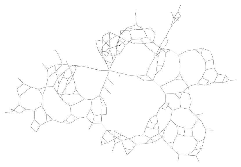
(a) ob-egl-g2-E

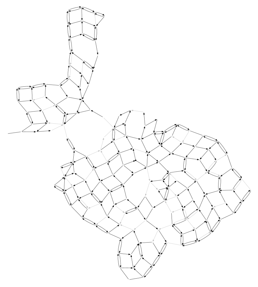
(b) ob-lpr-b-03

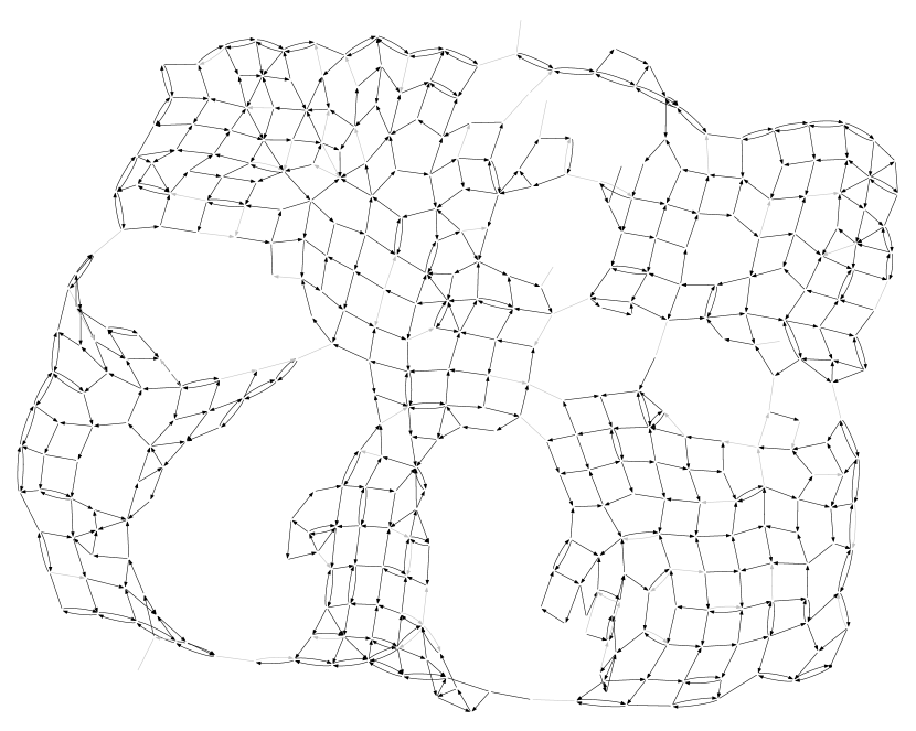
(c) ob2-lpr-b-05

Figure 5.1: Three instances from the Ob benchmark set.

5.3 The Ob benchmark set

Given our theoretical work in Sections 3 and 4, the solution quality achievable in polynomial time appears to mainly depend on the number $C$ on connected components in the graph induced by the positive-demand arcs. However, we noticed that widely used benchmark instances for variants of CARP have $C=1$. In order to motivate a more representative evaluation of the quality of polynomial-time heuristics for variants of CARP, we provide the Ob set of instances derived from the lpr and egl-large instances with $C$ from 2 to 5. The approach can be easily used to create more components.

The Ob instances simulate cities that are divided by a river that can be crossed via a few bridges without demand. The underlying assumption is that, for example, household waste does not have to be collected from bridges. We generated the instances as follows.

As a base, we took sufficiently large instances from the lpr and egl-large sets (it made little sense to split the small mval or lpr instances into several components). In each instance, we chose one or two random edges or arcs as “bridges”. Let $B$ be the set of their end points. We then grouped all vertices of the graph into clusters: For each $v\in B$, there is one cluster containing all vertices that are closer to $v$ than to all other vertices of $B$. Finally, we deleted all but a few edges between the clusters, so that usually two or three edges remain between each pair of clusters. The demand of the edges remaining between clusters is set to zero, they are our “bridges” between the river banks. The intuition is that, if one of our initially chosen edges or arcs $(u,v)$ was a bridge across a relatively straight river, then indeed every point on $u$’s side of the river would be closer to $u$ than to $v$. We discarded and regenerated instances that were not strongly connected or had river sides of highly imbalanced size (three times below the average component size). Figure 5.1 shows three of the resulting instances.

Note that this approach can yield instances where $C$ exceeds the number of clusters since deleting edges between the clusters may create more connected components in the graph induced by the positive-demand arcs. The approach straightforwardly applies to generating instances with even larger $C$: One simply chooses more initial “bridges”.

As a starting point, Table 5.3 shows the number $C$, a lower bound (LB) computed using an ILP relaxation of Gouveia et al. [27], and the best upper bound obtained using our approximation algorithm for each of the Ob instances using any of the service direction heuristics in Section 5.1.2. The “ob-” instances were generated by choosing one initial bridge, the “ob2-” instances were generated by choosing two initial bridges.

Table 5.3: First upper and lower bounds for the Ob instances described in Section 5.3.

Instance	$C$	LB	UB	Instance	$C$	LB	UB
ob-egl-g1-A	2	817 223	1 152 093	ob2-egl-g1-A	4	736 899	1 073 386
ob-egl-g1-B	2	1 180 105	1 627 305	ob2-egl-g1-B	5	840 773	1 221 424
ob-egl-g1-C	2	1 018 890	1 405 024	ob2-egl-g1-C	5	992 974	1 405 836
ob-egl-g1-D	3	1 354 671	1 810 306	ob2-egl-g1-D	4	1 056 593	1 491 387
ob-egl-g1-E	3	1 486 033	1 955 945	ob2-egl-g1-E	4	1 175 241	1 609 377
ob-egl-g2-A	2	922 853	1 286 986	ob2-egl-g2-A	4	854 823	1 202 379
ob-egl-g2-B	2	1 015 013	1 388 809	ob2-egl-g2-B	4	906 415	1 259 017
ob-egl-g2-C	2	1 308 463	1 701 004	ob2-egl-g2-C	4	1 154 372	1 574 762
ob-egl-g2-D	2	1 315 717	1 720 548	ob2-egl-g2-D	4	1 361 397	1 782 335
ob-egl-g2-E	2	1 677 109	2 139 982	ob2-egl-g2-E	4	1 295 704	1 747 883
ob-lpr-a-03	3	71 179	73 055	ob2-lpr-a-03	5	67 219	69 307
ob-lpr-a-04	2	119 759	123 838	ob2-lpr-a-04	4	115 110	119 550
ob-lpr-a-05	2	195 518	203 832	ob2-lpr-a-05	5	189 968	197 748
ob-lpr-b-03	2	73 670	75 052	ob2-lpr-b-03	5	67 924	69 518
ob-lpr-b-04	2	122 079	127 020	ob2-lpr-b-04	4	112 104	116 696
ob-lpr-b-05	2	204 389	213 593	ob2-lpr-b-05	5	191 138	197 878
ob-lpr-c-03	2	105 897	109 913	ob2-lpr-c-03	4	98 244	102 270
ob-lpr-c-04	2	161 856	167 336	ob2-lpr-c-04	4	155 894	161 615
ob-lpr-c-05	2	250 636	258 396	ob2-lpr-c-05	4	238 299	246 368

6 Conclusion

Since our algorithm outperforms many other polynomial-time heuristics, it is useful for computing good solutions in instances that are still too large to be attacked by exact, local search, or genetic algorithms. Moreover, it might be useful to use our solution as initial solution for local search algorithms.

Our theoretical results show that one should not evaluate polynomial-time heuristics only on instances whose positive-demand arcs induce a graph with only one connected component, because the solution quality achievable in polynomial time is largely determined by this number of connected components. Therefore, it would be interesting to see how other polynomial-time heuristics, which do not take into account the number of connected components in the graph induced by the positive-demand arcs, compare to our algorithm in instances where this number is larger than one.

Finally, we conclude with a theoretical question: It is easy to show a 3-approximation for the Mixed Chinese Postman problem using the approach in Section 3.3, yet Raghavachari and Veerasamy [37] showed a $3/2$-approximation. Can our $(\alpha(C)+3)$-approximation for MWRPP in Theorem 1.7(ii) be improved to an $(\alpha(C)+3/2)$-approximation analogously?

Acknowledgments.

This research was initiated during a research retreat of the algorithms and complexity theory group of TU Berlin, held in Rothenburg/Oberlausitz, Germany, in March 2015. We thank Sepp Hartung, Iyad Kanj, and André Nichterlein for fruitful discussions.

References

- Ahuja et al. [1993] R. K. Ahuja, T. L. Magnanti, and J. B. Orlin. Network Flows—Theory, Algorithms and Applications. Prentice Hall, 1993.
- Asadpour et al. [2010] A. Asadpour, M. X. Goemans, A. Mądry, S. O. Gharan, and A. Saberi. An -approximation algorithm for the asymmetric traveling salesman problem. In Proceedings of the 21st Annual ACM-SIAM Symposium on Discrete Algorithms (SODA’10), pages 379–389. Society for Industrial and Applied Mathematics, 2010. 10.1137/1.9781611973075.32.
- Beasley [1983] J. Beasley. Route first-Cluster second methods for vehicle routing. Omega, 11(4):403–408, 1983. 10.1016/0305-0483(83)90033-6.
- Belenguer et al. [2006] J.-M. Belenguer, E. Benavent, P. Lacomme, and C. Prins. Lower and upper bounds for the mixed capacitated arc routing problem. Computers & Operations Research, 33(12):3363–3383, 2006. 10.1016/j.cor.2005.02.009.
- Bellman [1962] R. Bellman. Dynamic programming treatment of the Travelling Salesman Problem. Journal of the ACM, 9(1):61–63, 1962. 10.1145/321105.321111.
- van Bevern et al. [2014a] R. van Bevern, S. Hartung, A. Nichterlein, and M. Sorge. Constant-factor approximations for capacitated arc routing without triangle inequality. Operations Research Letters, 42(4):290–292, 2014a. 10.1016/j.orl.2014.05.002.
- van Bevern et al. [2014b] R. van Bevern, R. Niedermeier, M. Sorge, and M. Weller. Complexity of arc routing problems. In Arc Routing: Problems, Methods, and Applications, MOS-SIAM Series on Optimization. SIAM, 2014b. 10.1137/1.9781611973679.ch2.
- van Bevern et al. [2015] R. van Bevern, C. Komusiewicz, and M. Sorge. Approximation algorithms for mixed, windy, and capacitated arc routing problems. In Proceedings of the 15th Workshop on Algorithmic Approaches for Transportation Modeling, Optimization, and Systems (ATMOS’15), volume 48 of OpenAccess Series in Informatics (OASIcs), pages 130–143. Schloss Dagstuhl–Leibniz-Zentrum für Informatik, 2015. 10.4230/OASIcs.ATMOS.2015.130.
- Bode and Irnich [2015] C. Bode and S. Irnich. In-depth analysis of pricing problem relaxations for the capacitated arc-routing problem. Transportation Science, 49(2):369–383, 2015. 10.1287/trsc.2013.0507.
- Brandão and Eglese [2008] J. Brandão and R. Eglese. A deterministic tabu search algorithm for the capacitated arc routing problem. Computers & Operations Research, 35(4):1112–1126, 2008. 10.1016/j.cor.2006.07.007.
- Christofides et al. [1986] N. Christofides, V. Campos, Á. Corberán, and E. Mota. An algorithm for the Rural Postman problem on a directed graph. In Netflow at Pisa, volume 26 of Mathematical Programming Studies, pages 155–166. Springer, 1986. 10.1007/BFb0121091.
- Corberán and Laporte [2014] Á. Corberán and G. Laporte, editors. Arc Routing: Problems, Methods, and Applications. SIAM, 2014.
- Corberán et al. [2000] A. Corberán, R. Martí, and A. Romero. Heuristics for the mixed rural postman problem. Computers & Operations Research, 27(2):183–203, 2000. 10.1016/S0305-0548(99)00031-3.
- Cygan et al. [2015] M. Cygan, F. V. Fomin, L. Kowalik, D. Lokshtanov, D. Marx, M. Pilipczuk, M. Pilipczuk, and S. Saurabh. Parameterized Algorithms. Springer, 2015. 10.1007/978-3-319-21275-3.
- Ding et al. [2014] H. Ding, J. Li, and K.-W. Lih. Approximation algorithms for solving the constrained arc routing problem in mixed graphs. European Journal of Operational Research, 239(1):80–88, 2014. 10.1016/j.ejor.2014.04.039.
- Dorn et al. [2013] F. Dorn, H. Moser, R. Niedermeier, and M. Weller. Efficient algorithms for Eulerian Extension and Rural Postman. SIAM Journal on Discrete Mathematics, 27(1):75–94, 2013. 10.1137/110834810.
- Downey and Fellows [2013] R. G. Downey and M. R. Fellows. Fundamentals of Parameterized Complexity. Springer, 2013. 10.1007/978-1-4471-5559-1.
- Edmonds [1975] J. Edmonds. The Chinese postman problem. Operations Research, pages B73–B77, 1975. Supplement 1.
- Edmonds and Johnson [1973] J. Edmonds and E. L. Johnson. Matching, Euler tours and the Chinese postman. Mathematical Programming, 5:88–124, 1973. 10.1007/BF01580113.
- Floyd [1962] R. W. Floyd. Algorithm 97: Shortest path. Communications of the ACM, 5(6):345, 1962. 10.1145/367766.368168.
- Frederickson [1977] G. N. Frederickson. Approximation Algorithms for NP-hard Routing Problems. PhD thesis, Faculty of the Graduate School of the University of Maryland, 1977.
- Frederickson [1979] G. N. Frederickson. Approximation algorithms for some postman problems. Journal of the ACM, 26(3):538–554, 1979. 10.1145/322139.322150.
- Frederickson et al. [1978] G. N. Frederickson, M. S. Hecht, and C. E. Kim. Approximation algorithms for some routing problems. SIAM Journal on Computing, 7(2):178–193, 1978. 10.1137/0207017.
- Frieze et al. [1982] A. M. Frieze, G. Galbiati, and F. Maffioli. On the worst-case performance of some algorithms for the asymmetric traveling salesman problem. Networks, 12(1):23–39, 1982. 10.1002/net.3230120103.
- Golden and Wong [1981] B. L. Golden and R. T. Wong. Capacitated arc routing problems. Networks, 11(3):305–315, 1981. 10.1002/net.3230110308.
- Golden et al. [1983] B. L. Golden, J. S. Dearmon, and E. K. Baker. Computational experiments with algorithms for a class of routing problems. Computers & Operations Research, 10(1):47–59, 1983. 10.1016/0305-0548(83)90026-6.
- Gouveia et al. [2010] L. Gouveia, M. C. Mourão, and L. S. Pinto. Lower bounds for the mixed capacitated arc routing problem. Computers & Operations Research, 37(4):692–699, 2010. 10.1016/j.cor.2009.06.018.
- Gutin et al. [2016] G. Gutin, M. Wahlström, and A. Yeo. Rural Postman parameterized by the number of components of required edges. Journal of Computer and System Sciences, 2016. 10.1016/j.jcss.2016.06.001. In press.
- Hall [1935] P. Hall. On representatives of subsets. Journal of the London Mathematical Society, 10:26–30, 1935. 10.1112/jlms/s1-10.37.26.
- Held and Karp [1962] M. Held and R. M. Karp. A dynamic programming approach to sequencing problems. Journal of the Society for Industrial and Applied Mathematics, 10(1):196–210, 1962. 10.1137/0110015.
- Jansen [1993] K. Jansen. Bounds for the general capacitated routing problem. Networks, 23(3):165–173, 1993. 10.1002/net.3230230304.
- Lenstra and Rinnooy Kan [1976] J. K. Lenstra and A. H. G. Rinnooy Kan. On general routing problems. Networks, 6(3):273–280, 1976. 10.1002/net.3230060305.
- Marx [2008] D. Marx. Parameterized complexity and approximation algorithms. The Computer Journal, 51(1):60–78, 2008. 10.1093/comjnl/bxm048.
- Mourão and Amado [2005] M. C. Mourão and L. Amado. Heuristic method for a mixed capacitated arc routing problem: A refuse collection application. European Journal of Operational Research, 160(1):139–153, 2005. 10.1016/j.ejor.2004.01.023.
- Orloff [1976] C. S. Orloff. On general routing problems: Comments. Networks, 6(3):281–284, 1976. 10.1002/net.3230060306.
- Pearn and Wu [1995] W. L. Pearn and T. C. Wu. Algorithms for the rural postman problem. Computers & Operations Research, 22(8):819–828, 1995. 10.1016/0305-0548(94)00070-O.
- Raghavachari and Veerasamy [1999] B. Raghavachari and J. Veerasamy. A 3/2-approximation algorithm for the Mixed Postman Problem. SIAM Journal on Discrete Mathematics, 12(4):425–433, 1999. 10.1137/S0895480197331454.
- Sorge et al. [2011] M. Sorge, R. van Bevern, R. Niedermeier, and M. Weller. From few components to an Eulerian graph by adding arcs. In Proceedings of the 37th International Workshop on Graph-Theoretic Concepts in Computer Science (WG’11), pages 307–318. Springer, 2011. 10.1007/978-3-642-25870-1_28.
- Sorge et al. [2012] M. Sorge, R. van Bevern, R. Niedermeier, and M. Weller. A new view on Rural Postman based on Eulerian Extension and Matching. Journal of Discrete Algorithms, 16:12–33, 2012. 10.1016/j.jda.2012.04.007.
- Ulusoy [1985] G. Ulusoy. The fleet size and mix problem for capacitated arc routing. European Journal of Operational Research, 22(3):329–337, 1985. 10.1016/0377-2217(85)90252-8.
- Wøhlk [2008] S. Wøhlk. An approximation algorithm for the Capacitated Arc Routing Problem. The Open Operational Research Journal, 2:8–12, 2008. 10.2174/1874243200802010008.