Passive advection of a vector field: Anisotropy, finite correlation time, exact solution and logarithmic corrections to ordinary scaling

Abstract

In this work we study the generalization of the problem, considered in [Phys. Rev. E 91, 013002 (2015)], to the case of finite correlation time of the environment (velocity) field. The model describes a vector (e.g., magnetic) field, passively advected by a strongly anisotropic turbulent flow. Inertial-range asymptotic behavior is studied by means of the field theoretic renormalization group and the operator product expansion. The advecting velocity field is Gaussian, with finite correlation time and preassigned pair correlation function. Due to the presence of distinguished direction ${\bf n}$, all the multiloop diagrams in this model are vanish, so that the results obtained are exact. The inertial-range behavior of the model is described by two regimes (the limits of vanishing or infinite correlation time) that correspond to the two nontrivial fixed points of the RG equations. Their stability depends on the relation between the exponents in the energy spectrum ${\cal E}\propto k_{\bot}^{1-\xi}$ and the dispersion law $\omega\propto k_{\bot}^{2-\eta}$. In contrast to the well known isotropic Kraichnan’s model, where various correlation functions exhibit anomalous scaling behavior with infinite sets of anomalous exponents, here the corrections to ordinary scaling are polynomials of logarithms of the integral turbulence scale $L$.

I Introduction

Over decades much attention has been paid to the problem of intermittency and anomalous scaling in fully developed turbulence. Both the natural experiments and numerical simulations suggest that the violation of the classical Kolmogorov–Obukhov theory Legacy is even more strongly pronounced for a advected field than for the velocity field itself; see, e.g., Advection ; FGV and references therein. At the same time, the problem of passive advection appears to be easier tractable theoretically. Although the theoretical description of the fluid turbulence on the basis of the stochastic Navier–Stokes (NS) equations remains essentially an open problem, considerable progress has been achieved in understanding passive advection by random “synthetic” velocity fields. The most remarkable progress has been achieved for the so-called Kraichnan’s rapid-change model Kraich1 , in which the velocity field is modeled by Gaussian ensemble, not correlated in time, with zero mean and pair correlation function of the form

$$\langle v_{i}(x)v_{j}(x^{\prime})\rangle=\delta(t-t^{\prime})\,D_{0}\ \int_{k>m}\frac{d{\bf k}}{(2\pi)^{d}}\,P_{ij}({\bf k})\,\frac{1}{k^{d+\xi}}\ e^{{\rm i}{\bf k}\cdot({\bf x}-{\bf x^{\prime}})}.$$ (1)

Here $P_{ij}({\bf k})=\delta_{ij}-k_{i}k_{j}/k^{2}$ is the transverse projector, $k\equiv|{\bf k}|$, $D_{0}>0$ is an amplitude factor, $d$ is the dimensionality of the ${\bf x}$ space and $0<\xi<2$ is a parameter with the real (“Kolmogorov”) value $\xi=4/3$. For the first time, the anomalous exponents have been calculated on the basis of a microscopic model and within regular expansions in formal small parameters FGV .

A passively advected field may be chosen both scalar and vector, the latter case corresponds to the magnetohydrodynamic (MHD) turbulence. From the experimental point of view it is a special problem, closely related to the processes taken place in solar corona, e.g., with solar wind; for detailed discussion see GM-mod ; E ; SW2 and references therein.

In solar flares, highly energetic and anisotropic large-scale motions coexist with small-scale coherent structures, finally responsible for the dissipation. A simplified description of the situation was proposed in E : the large-scale field $B^{0}_{i}=n_{i}B^{0}$ dominates the dynamics in the distinguished direction ${\bf n}$, while the activity in the perpendicular plane is described as nearly two-dimensional.

The observations and simulations show that the scaling behavior in the solar wind is closer to the anomalous scaling of the three-dimensional fully developed hydrodynamic turbulence, rather than to simple Iroshnikov-Kraichnan scaling suggested by the two-dimensional picture with the inverse energy cascade SW2 . Thus, further analysis of more realistic three-dimensional models is welcome.

One of the possibilities to make original Kraichnan’s model (1) anisotropic is to replace the ordinary transverse projector with the tensor quantity $T_{ij}({\bf k})$, which contains a fixed unit vector ${\bf n}$:

$$T_{ij}({\bf k})=a(\psi)P_{ij}({\bf k})+b(\psi)n_{s}n_{l}P_{is}({\bf k})P_{jl}({\bf k}),$$ (2)

where $a(\psi)$ and $b(\psi)$ are some functions of $\psi$, the angle between the vectors ${\bf n}$ and ${\bf k}$; see, e.g., Uni ; Uni2 ; Uni3 . This formulation of the problem corresponds to the small-scale anisotropy and contains an isotropic model as a special case, if $a(\psi)=1$ and $b(\psi)=0$.

Another possibility is the “strongly anisotropic” model that does not contain an isotropic one as a special case and is obtained by introducing the velocity field ${{\bm{v}}}$ having preferred direction ${\bf n}$:

$$\bm{v}(t,{\bf x})={\bf n}\times v(t,\ {\bf x_{\perp}}).$$ (3)

In this paper, we consider a more realistic model with finite (and not small) correlation time. For this purpose the correlation function (1) has to be modified, and instead of a constant, which is Fourier transform of $\delta(t-t^{\prime})$, in the frequency space it becomes a function of $\omega$. In common cases this modification disrupts the Galilean invariance FinTime-GalileanLack and is interesting only as a model, but in the presence of the anisotropy Galilean invariance survives and the model is invariant under some special Galilean transformations (more precisely see below).

The energy spectrum of the velocity in the inertial range has the form ${\cal E}\propto k_{\bot}^{1-\xi}$, while the correlation time at the momentum $k$ scales as $k^{-2+\eta}$. Such ensemble was employed in some models, studied in FinTime ; FinTimeEta . It was shown that, depending on the values of the exponents $\xi$ and $\eta$, the model reveals various types of inertial-range scaling regimes with nontrivial anomalous exponents, which were explicitly derived to the first FinTime and second FinTimeEta orders of the double expansion in $\xi$ and $\eta$.

It is necessity to stress, that the Kraichnan’s model (1) and its generalizations correspond to passive field approximation: if we neglect the influence of advected field $\bm{\theta}$ to the dynamics of the environment (velocity) field ${{\bm{v}}}$, the latter can be modeled by statistical ensembles with prescribed properties. This approximation is valid when the gradients of the magnetic fields are not too large.

A most powerful method to study the anomalous scaling in various statistical models of turbulent advection provided by the field theoretic renormalization group (RG) and operator product expansion (OPE); see the monographs Zinn ; Vasiliev-Green and references therein. In the RG+OPE scenario RG , anomalous scaling emerges as a consequence of the existence in the model of composite fields (“composite operators” in the quantum-field terminology) with negative scaling dimensions; see JphysA for a review and the references. In a number of papers the RG+OPE approach was applied to the case of passive vector (magnetic) fields in Kraichnan’s ensemble, and to its generalizations (large-scale anisotropy, helicity, compressibility, finite correlation time, non-Gaussianity, more general form of the nonlinearity); see Lanotte2-mod ; AntGul2012-mod ; Marian ; Marian2 ; Kotumay and references therein. Explicit analytical expressions were derived for the anomalous exponents to the first Lanotte2-mod and the second AntGul2012-mod ; Marian orders in $\xi$. For the pair correlation function of the magnetic field, exact results were obtained within the zero-mode approach V96-mod .

In this paper, we apply the field theoretic renormalization group and operator product expansion to the inertial-range behavior of strongly anisotropic MHD turbulence within the framework of a simplified model, which corresponds to the problem of a passive vector field advected by the Gaussian ensemble with prescribed statistics. The velocity field ${{\bm{v}}}$ is chosen to be oriented along a fixed direction ${\bf n}$ (“orientation of a large-scale flare” in the context of the solar corona dynamics) and depends only on the coordinates in the subspace orthogonal to ${\bf n}$. In the momentum space, its correlation function is some function of $k_{\bot}$ and frequency $\omega$, where $k_{\bot}=|{\bf k}_{\bot}|$ and ${\bf k}_{\bot}$ is the component of the momentum (wave number) ${\bf k}$ perpendicular to ${\bf n}$. This model can be viewed as a $d$-dimensional generalization of the strongly anisotropic velocity ensemble introduced in AM in connection with the turbulent diffusion problem and further studied and generalized in a number of papers AM1-mod ; AM5-mod ; Glimm-mod ; Foba ; AntMal2011 .

The advecting equation for the passive field $\bm{\theta}$ involves a general relative coefficient ${\cal A}$, which unifies different physical situations: the kinematic MHD model, the linearized NS equation and the passive admixture with complex internal structure of the particles.

In AntMal2011 the problem of anomalous scaling in the higher-order correlation functions of a scalar field, advected by such a velocity ensemble, was studied by the RG+OPE techniques. It was shown that there exists some set of fixed points, which governs infrared (IR) behavior of the system. Another conclusion of that work is that in sharp contrast to the isotropic Kraichnan’s model and its numerous descendants, due to the mixing of families of relevant composite operators the correlation functions show no anomalous scaling and have finite limits when the integral turbulence scale tends to infinity.

Further modification of that problem, namely advection of the vector field by decorrelated in time velocity field, was studied in VectorN . In contrast to AntMal2011 , the inertial-range behavior of vector fields appears to be even more exotic: instead of power-like anomalies, there are logarithmic corrections to ordinary scaling, determined by naive (canonical) dimensions.

The main result of the present paper is that the inertial-range behavior of vector fields advected by velocity ensemble with finite correlation time combines both the above features: as in the scalar case, there is a set of fixed points, governing the IR behavior; as in the zero-time correlation model, the inertial-range behavior of vector fields has logarithmic corrections to ordinary scaling. The key point is that the matrices of scaling dimensions (“critical dimensions” in the terminology of the theory of critical state) of the relevant families of composite operators appear nilpotent and cannot be diagonalized. They can only be brought to Jordan form; hence the logarithms.

Another interesting property, inherited from the zero-time correlation model, is that all multiloop diagrams are equal to zero and therefore the set of fixed points and the existence of logarithmic corrections are proven exactly. Moreover, in contrast to previous one, this model has two types of such nontrivial diagrams, with different causes to be equal to zero. The physical meaning of this feature is not yet clarified, but it is clear that it is closely connected with the presence of the anisotropy vector ${\bf n}$.

The paper is organized as follows.

In Sec. II we give a detailed description of the model. In Sec. III we present the field theoretic formulation of the model and the corresponding diagrammatic techniques. In Sec. IV we establish renormalizability of the model and derive explicit exact expressions for the renormalization constants and RG functions (anomalous dimensions and $\beta$-functions). Due to the presence of the anisotropy, the linear response function, the only Green function in the model that contains superficial ultraviolet (UV) divergences, is given exactly by the one-loop approximation.

It is shown that the IR behavior of the model is confined with only two limiting cases: the rapid-change type behavior and the “frozen” (time-independent) behavior. In contrast to the isotropic case, where the physical (Kolmogorov) point $\xi=8/3$, $\eta=4/3$ lies exactly on the crossover line between the rapid-change and frozen regimes FinTime ; FinTimeEta ; Chetak , now this point lies deep inside the domain of stability of the nontrivial rapid-change behavior; there is no crossover line going through this point. This result is in agreement with the exact analysis of the $d=(1+1)$-dimensional case Glimm-mod and in disagreement with AM ; AM1-mod .

The corresponding differential equations of IR scaling are derived, with the exactly known critical dimensions.

In Sec. V we discuss the renormalization of composite operators and present explicit expressions for the matrices of anomalous dimensions and critical dimensions. It is shown that these matrices are given exactly by the one-loop approximation. The matrices of anomalous dimensions appear to be nilpotent. As a result, the IR behavior of the pair correlation functions of the composite operators is given by canonical powers, corrected by polynomials of logarithms. To obtain inertial-range behavior we have to combine this result with the corresponding OPE’s. Finally, asymptotic behavior of the pair correlation functions involves two types of large logarithms, where the separation enters with the typical UV and IR scales (dissipation scale and integral scale).

Sec. VI is reserved for conclusions.

II Description of the model

If the field $\bm{v}$ is chosen in the strongly anisotropic form (3), the turbulent advection of a passive vector field $\bm{\theta}(x)\equiv\bm{\theta}(t,{\bf x})$ is described by the stochastic equation VectorN ; Ant-Hnat-Hon-Jut-11

$$\partial_{t}\theta_{i}+\partial_{k}\left(v_{k}\theta_{i}-{\cal A}_{0}\ v_{i}\theta_{k}\right)+\partial{\cal P}=\nu_{0}\ (\partial_{\perp}^{2}+f_{0}\partial_{\parallel}^{2})\theta_{i}+f_{i},$$ (4)

where $\theta_{i}(x)$ is a vector field, $x\equiv\left\{t,{\bf x}\right\}$, $\partial_{t}\equiv\partial/\partial t$, $\partial_{i}\equiv\partial/\partial x_{i}$, ${\bf n}$ is a unit vector that determines the distinguished direction, ${\bf x}_{\bot}$ and $\bm{\partial}_{\perp}$ are the components of the vectors ${\bf x}$ and $\bm{\partial}$ perpendicular to ${\bf n}$, $\partial_{\parallel}\equiv\bm{\partial}\cdot{\bf n}$, $\nu_{0}$ is the molecular diffusivity coefficient, $\partial^{2}$ is the Laplace operator, $\bm{v}(x)\equiv\{v_{i}(x)\}$ is the velocity field, $f_{i}\equiv f_{i}(x)$ is an artificial Gaussian scalar noise with zero mean and correlation function

$$\left\langle f_{i}(t,\ {\bf x})\ f_{k}(t^{\prime},\ {\bf x^{\prime}})\right\rangle=\delta(t-t^{\prime})\ C_{ik}({\bf r}/L).$$ (5)

Here ${\bf r=x-x^{\prime}}$, $r=\left|{\bf r}\right|$, the parameter $L\equiv M^{-1}$ is the integral (external) turbulence scale related to the stirring, and $C_{ik}$ is a dimensionless function finite for $r/L\to 0$ and rapidly decaying for $r/L\to\infty$.

Both $\bm{v}$ and ${\bm{\theta}}$ are divergence-free (“solenoidal”) vector fields:

$$\partial_{i}v_{i}=0,\quad\partial_{i}\theta_{i}=0.$$ (6)

Following amodel , we included into the stochastic advection-diffusion equation (4) additional arbitrary dimensionless parameter ${\cal A}_{0}$, which unifies different physical situations: the case ${\cal A}_{0}=1$ corresponds to the kinematic MHD equation, describing, for example, the evolution of the fluctuating part ${\bm{\theta}}\equiv{\bm{\theta}}(x)$ of the magnetic field in the presence of a mean component ${\bm{\theta}}^{0}$, which is supposed to be varying on a very large scale; the case ${\cal A}_{0}=-1$ corresponds to the linearization of the NS equation around the rapid-change background velocity field; in the case ${\cal A}_{0}=0$ equation (4) loses the stretching term $\partial_{k}(v_{i}\theta_{k})$ and the model acquires additional symmetry under translations ${\bm{\theta}}\to{\bm{\theta}+const}$. This case has to be studied separately, see Matraz .

The pressure term can be expressed as the solution of the Poisson equation

$$\partial^{2}{\cal P}=({\cal A}_{0}-1)\,\partial_{i}v_{k}\partial_{k}\theta_{i}$$ (7)

and is needed to reconcile dynamics of the field $\theta_{i}$ with transversality condition (6).

For renormalizability reasons it is necessary to introduce additional dimensionless constant $f_{0}$, which breaks the $O_{d}$ symmetry of the Laplace operator to $O_{d-1}\otimes Z_{2}$: $\partial^{2}\rightarrow\ \partial_{\perp}^{2}+f_{0}\partial_{\parallel}^{2}$ ($Z_{2}$ is the reflection symmetry $x_{\parallel}\to-x_{\parallel}$). Interpretation of the splitting of the Laplacian term can be twofold; cf. AntMal2011 . On one hand, stochastic models of the type (4) must include all the IR relevant terms allowed by the symmetry, therefore it is natural to include the general value $f_{0}\neq 1$ to the model from the very beginning. On the other hand, the extension of the model to the case $f_{0}\neq 1$ can be viewed as a purely technical trick which is only needed to ensure the multiplicative renormalizability and to derive the RG equations.

Instead of the real problem, where the velocity field $\bm{v}(x)$ has to satisfy the NS equation with some additional terms that describe the feedback of the advected field $\bm{\theta}(x)$ on the velocity field, we will consider the kinematic problem, where the reaction of the field $\bm{\theta}(x)$ on the velocity field $\bm{v}(x)$ is neglected. It is assumed that, if the gradients of $\bm{\theta}(x)$ are not too large, it does not affect essentially dynamics of the conducting fluid. Thus, the field $\bm{v}(x)$ can be simulated by statistical ensemble with prescribed statistics. It is assumed to be Gaussian, strongly anisotropic [see (3)], homogeneous, with zero mean and a correlation function FinTime ; FinTimeEta ; AntMal2011

$$\left\langle v_{i}(t,\ {\bf x})\ v_{k}(t^{\prime},\ {\bf x^{\prime}})\right\rangle=n_{i}n_{k}\ \left\langle v(t,\ {\bf x_{\perp}})\ v(t^{\prime},\ {\bf x^{\prime}_{\perp}})\right\rangle,$$ (8)

where

$$\left\langle v(t,\ {\bf x_{\perp}})\ v(t^{\prime},\ {\bf x^{\prime}_{\perp}})\right\rangle=\int_{k>m}\frac{d{\bf k}}{(2\pi)^{d}}\ e^{i{\bf k\cdot(x-x^{\prime})}}\ D_{v}(\omega,k).$$ (9)

The function $D_{v}$ is chosen in the form

$$D_{v}(\omega,k)=2\pi\delta(k_{\parallel})\ D_{0}\ \frac{k_{\perp}^{5-d-(\xi+\eta)}}{\omega^{2}+\left[\alpha_{0}\nu_{0}k_{\perp}^{2-\eta}\right]^{2}}.$$ (10)

Here $d$ is the dimensionality of the ${\bf x}$ space, $k_{\perp}\equiv|{\bf k_{\perp}}|$, $1/m$ is another integral turbulence scale, related to the stirring, $D_{0}>0$ is an amplitude factor and symbol $k_{\parallel}$ denotes the scalar product ${\bf k\cdot n}$. The function (9) involves two independent exponents $\xi$ and $\eta$, which in the RG approach play the role of two formal expansion parameters; a new parameter $\alpha_{0}$ is needed for the dimensionality reason. Depending of this parameter, the function (10) demonstrates two interesting limiting cases: if $\alpha_{0}\to 0$, $D_{v}(\omega)\propto\delta(\omega)$, so that from the physs point of view this situation corresponds to the independent of time (“frozen”) velocity field. The situation $\alpha_{0}\to\infty$ in fact means that $(\alpha_{0}\nu_{0})^{2}\gg\omega^{2}$, so that this case corresponds to the rapid-change model.

The relations

$$D_{0}/\nu_{0}^{3}f_{0}=\tilde{g}_{0}\equiv\Lambda^{\xi+\eta}$$ (11)

define the coupling constant $\tilde{g}_{0}$, which plays the role of the expansion parameter in the ordinary perturbation theory, and the characteristic UV momentum scale $\Lambda$.

III Field theoretic formulation of the model

III.1 The action functional and the Galilean symmetry

The stochastic problem (4) – (10) is equivalent to the field theoretic model of the extended set of three fields $\Phi\equiv\left\{\bm{\theta},\bm{\theta}^{\prime},\bm{v}\right\}$ with the action functional

$${\cal S}(\Phi)=-\frac{1}{2}v_{i}D_{v}^{-1}v_{k}+\frac{1}{2}\theta^{\prime}_{i}D_{\theta}\theta^{\prime}_{k}+\theta^{\prime}_{k}\left[-\partial_{t}\theta_{k}-(v_{i}\partial_{i})\theta_{k}+{\cal A}_{0}(\theta_{i}\partial_{i})v_{k}+\nu_{0}(\partial_{\perp}^{2}+f_{0}\partial_{\parallel}^{2})\theta_{k}\right].$$ (12)

Here all the terms, with the exception of the first one, represent the De Dominicis–Janssen action for the stochastic problem (4), (5) at fixed $\bm{v}$, while the first term represents the Gaussian averaging over $\bm{v}$. Furthermore, $D_{\theta}$ and $D_{v}$ are the correlators (5) and (8) respectively; the needed integrations over $x=(t,{\bf x})$ and summations over the vector indices are implied.

As a rule, synthetic velocity ensembles with finite correlation time suffer from the lack of Galilean invariance, which can lead to some physical pathologies; see, e.g., the discussion in FinTime-GalileanLack . Surprisingly enough, the presence of the anisotropy can improve the situation.

Indeed, it is directly checked that in our strongly anisotropic case the action functional (12) with the correlator (8) in its first term appears invariant with respect to the Galilean transformation of a special form:

$$\theta(t,{\bf x}) \to \theta(t,{\bf x}+{{\bm{u}}}t),\quad\theta^{\prime}(t,{\bf x})\to\theta^{\prime}(t,{\bf x}+{{\bm{u}}}t),$$

$${{\bm{v}}}(t,{\bf x}) \to {{\bm{v}}}(t,{\bf x}+{{\bm{u}}}t)-{{\bm{u}}}.$$ (13)

Here the transformation parameter has the form ${{\bm{u}}}={\bf n}u$ with the vector ${\bf n}$ from (3), so that the scalar coefficient in (3) changes as $v(t,{\bf x}_{\bot})\to v(t,{\bf x}_{\bot})-u$ and the arguments ${\bf x}_{\bot}$ of all the fields in (13) remain intact.

This fact can be interpreted as follows. Consider the generalized stochastic NS equation

$$\partial_{t}v_{i}+(v_{l}\partial_{l})v_{i}+\partial_{i}\wp=Rv_{i}+\phi_{i},$$ (14)

where $R$ is some differential operation acting only on spatial coordinates and $\wp=-\partial^{-2}(\partial_{i}v_{l})(\partial_{l}v_{i})$ is the pressure. If the random force $\phi_{i}$ is taken to be white in time, the equation (14) is Galilean covariant because it involves the full covariant derivative $\partial_{t}+(v_{l}\partial_{l})$.

However, for the velocity field of the form (3) all the nonlinear terms in (14) vanish due to the independence of the scalar coefficient $v$ on $x_{\parallel}$: $v_{k}\partial_{k}v_{i}=n_{i}v\partial_{\parallel}v=0$, and similarly for the pressure. Thus the equation (14) becomes in fact linear and generates a Gaussian velocity field. Its pair correlation function has the form

$$\left\langle v_{i}v_{j}\right\rangle=\frac{D^{\phi}_{ij}({\bf k})}{\omega^{2}+R^{2}({\bf k})},$$ (15)

where $D^{\phi}_{ij}({\bf k})$ is the pair correlator of the random force $\phi_{i}$. It coincides with (8) if one choses (in the momentum representation) $R({\bf k})=u_{0}\nu_{0}k_{\bot}^{2-\eta}$ and $\phi_{i}=\phi n_{i}$ with $\langle\phi\phi\rangle=g_{0}\nu_{0}^{3}f_{0}\,\delta(t-t^{\prime})\,\delta(k_{\parallel})k_{\bot}^{5-d-(\varepsilon+\eta)}$. It remains to note that the resulting velocity ensemble has a finite correlation time in contrast to the random force $\phi_{i}$ in (14).

III.2 Feynman diagrammatic technique

The model (12) corresponds to a standard Feynman diagrammatic technique with the triple vertex $\theta^{\prime}\left[-(v_{i}\partial_{i})\theta_{k}+{\cal A}_{0}(\theta_{i}\partial_{i})v_{k}\right]$ and the three bare propagators. A fragment of arbitrary diagram is represented in Fig. (1).

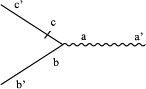
Figure 1: The triple vertex with three attached propagators.

In the frequency-momentum representation the triple vertex corresponds to the expression

$$V_{c\,ab}=i\delta_{bc}\ k_{a}^{\theta^{\prime}}-i{\cal A}_{0}\delta_{ac}\ k_{b}^{\theta^{\prime}},$$ (16)

where $k^{\theta^{\prime}}$ is the momentum of the field $\theta^{\prime}$; in the diagrams it is represented by the point, in which three lines connect with each other. The three propagators are determined by the quadratic (free) part of the action functional and are represented in the diagrams as slashed straight (the slashed end corresponds to the field $\theta^{\prime}$), straight (the end without a slash corresponds to the field $\theta$) and wavy (which corresponds to the field $v$) lines, respectively; cf. VectorN .

The line $\left\langle v_{a}v_{a^{\prime}}\right\rangle_{0}$ in the diagrams corresponds to the correlation function (8), and the other two propagators in the frequency-momentum representation have the forms

$$\left\langle\theta_{c}\theta^{\prime}_{c^{\prime}}\right\rangle_{0} = \frac{P_{cc^{\prime}}({\bf k})}{-i\omega+\nu_{0}\left({\bf k}_{\perp}^{2}+f_{0}k_{\parallel}^{2}\right)},$$ (17)

$$\left\langle\theta_{b}\theta_{b^{\prime}}\right\rangle_{0} = \frac{C_{bb^{\prime}}({\bf k})}{\omega^{2}+\left[\nu_{0}\left({\bf k}_{\perp}^{2}+f_{0}k_{\parallel}^{2}\right)\right]^{2}}.$$ (18)

Here $C_{bb^{\prime}}({\bf k})\propto P_{bb^{\prime}}({\bf k})$ is the Fourier transform of the function from (5); the propagator $\left\langle\theta^{\prime}_{d}\theta^{\prime}_{d^{\prime}}\right\rangle$ is equal to zero.

In fact, the action functional (12) has to be modified for the sake of renormalizability. As a consequence, the functions (17) and (18) will acquire certain additional terms. However, it turns out that those additional terms do not contribute to the divergent parts of all the relevant diagrams, and thus they can be neglected. These issues are discussed in detail in sec. IV.4, and in the following we will use for the propagators the above expressions (17) and (18).

III.3 Canonical dimensions and UV divergences

The analysis of UV divergences is based on the analysis of canonical dimensions of the 1-irreducible Green functions. In general, dynamic models have two scales: canonical dimension of some quantity $F$ (a field or a parameter in the action functional) is completely characterized by two numbers, the frequency dimension $d_{F}^{\omega}$ and the momentum dimension $d_{F}^{k}$. They are defined such that

$$[F]\sim[T]^{-d_{F}^{\omega}}[L]^{-d_{F}^{k}},$$ (19)

where $L$ is some reference length scale and $T$ is a time scale.

In the scalar version of strongly anisotropic model (3) – (10), however, there are two independent length scales, related to the directions perpendicular and parallel to the vector ${\bf n}$ AntMal2011 . But the transversality conditions

$$\partial_{i}\theta_{i}=0,\quad\partial_{i}\theta^{\prime}_{i}=0$$ (20)

forbid this option; see VectorN . In particular, this means that, in contrast to the scalar case, the constant $f_{0}$ from (4) in our case is dimensionless.

The dimensions in (19) are found from the obvious normalization conditions $d_{k}^{k}=-d_{\bf x}^{k}=1$, $d_{k}^{\omega}=-d_{\bf x}^{\omega}=0$, $d_{\omega}^{\omega}=-d_{t}^{\omega}=1$, $d_{\omega}^{k}=d_{t}^{k}=0$, and from the requirement that each term of the action functional (12) be dimensionless (with respect to the two independent dimensions separately). Based on $d_{F}^{k}$ and $d_{F}^{\omega}$, one can introduce the total canonical dimension $d_{F}=d_{F}^{k}+2d_{F}^{\omega}$ (in the free theory, $\partial_{t}\propto\partial^{2}_{\bot}\propto\partial^{2}_{\parallel}$), which plays in the theory of renormalization of dynamic models the same role as the conventional (momentum) dimension does in static problems; see, e.g., Vasiliev-Green .

Table 1: Canonical dimensions of the fields and parameters

$F$	$\theta^{\prime}$	$\theta$	$\bm{v}$	$M,m,\mu,\Lambda$	$\nu,\nu_{0}$	${\cal A},{\cal A}_{0}$	$f,f_{0}$	$u,u_{0}$	$\alpha_{0}$	$\tilde{g}_{0}$, $g_{0}$	$\alpha$, $\tilde{g}$, $g$
$d_{F}^{\omega}$	1/2	$-1/2$	1	0	1	0	0	0	0	0	0
$d_{F}^{k}$	$d$	0	$-1$	1	$-2$	0	0	0	$\eta$	$\xi+\eta$	0
$d_{F}$	$d+1$	$-1$	1	1	0	0	0	0	$\eta$	$\xi+\eta$	0

The canonical dimensions for the model (12) are given in Table 1, including renormalized parameters, which will be introduced a bit later. From Table 1 it follows that our model is logarithmic (the coupling constants $g_{0}\sim[L]^{-\xi-\eta}$ and $\alpha_{0}\sim[L]^{-\eta}$ are dimensionless) at $\xi=\eta=0$, so that the UV divergences in the Green functions manifest themselves as poles in $\xi$, $\eta$ and their linear combinations.

The total canonical dimension of an arbitrary 1-irreducible Green function $\Gamma_{N_{\Phi}}=\langle\Phi\dots\Phi\rangle_{\rm 1-ir}$ is given by the relation

$$d_{\Gamma_{N_{\Phi}}}=d+2-\sum_{\Phi}N_{\Phi}d_{\Phi}=d+2-N_{\theta^{\prime}}d_{\theta^{\prime}}-N_{\theta}d_{\theta}-N_{v}d_{v}.$$ (21)

Here $N_{\Phi}=\{N_{\theta},\,N_{\theta^{\prime}},\,N_{v}\}$ are the numbers of corresponding fields entering the function $\Gamma_{N_{\Phi}}$, and the summation over all types of the fields in (21) and analogous formulae below is always implied.

Superficial UV divergences, whose removal requires counterterms, can be present only in those functions $\Gamma_{N_{\Phi}}$ for which the “formal index of divergence” $d_{\Gamma_{N_{\Phi}}}$ is a non-negative integer. Dimensional analysis should be augmented by the following considerations:

(1) In any dynamical model of type (12), 1-irreducible diagrams with $N_{\theta^{\prime}}=0$ necessarily contain closed circuits of retarded propagators (17) or at least one vanishing propagator $\left\langle\theta_{i}^{\prime}\theta_{k}^{\prime}\right\rangle$ and therefore vanish.

(2) For any 1-irreducible Green function $N_{\theta^{\prime}}-N_{\theta}=2N_{0}$, where $N_{0}\geq 0$ is the total number of the bare propagators $\langle\theta\theta\rangle_{0}$ entering into any of its diagrams.

(3) Using the transversality condition of the fields $\theta_{i}$ and $v_{i}$ we can move one derivative from the vertex $-\theta^{\prime}_{k}(v_{i}\partial_{i})\theta_{k}+{\cal A}_{0}\ \theta^{\prime}_{k}(\theta_{i}\partial_{i})v_{k}$ onto the field $\theta^{\prime}_{i}$. Therefore, in any 1-irreducible diagram it is always possible to move the derivative onto external “tail” $\theta^{\prime}_{k}$, which reduces the real index of divergence: $d_{\Gamma_{N_{\Phi}}}^{\prime}=d_{\Gamma_{N_{\Phi}}}-N_{\theta^{\prime}}$. The field $\theta^{\prime}_{k}$ enters the counterterms only in the form of the derivative $\partial_{i}\theta^{\prime}_{k}$.

From Table 1 and (21) we find that

$$d_{\Gamma_{N_{\Phi}}}=d+2-(d+1)N_{\theta^{\prime}}+N_{\theta}-N_{v}$$ (22)

and

$$d^{\prime}_{\Gamma_{N_{\Phi}}}\!=(d+2)(1-N_{\theta^{\prime}})+N_{\theta}-N_{v}.$$ (23)

From these expressions we conclude that, for any $d$, superficial divergences can be present only in the 1-irreducible functions of two types.

The first example is provided by the infinite family of functions $\langle\theta^{\prime}\theta\dots\theta\rangle_{\rm 1-ir}$ with $N_{\theta^{\prime}}=1$ and arbitrary $N_{\theta}$, for which $d_{\Gamma}=2$, $d_{\Gamma}^{\prime}=0$. However, all the functions with $N_{\theta}\geq N_{\theta^{\prime}}$ vanish (see above) and obviously do not require counterterms. Therefore the only nonvanishing function from this family is $\langle\theta_{\alpha}^{\prime}\theta_{\beta}\rangle_{\rm 1-ir}$.

Another possibility is $\langle\theta^{\prime}\theta\dots\theta v\dots v\rangle_{\text{1-ir}}$ with $N_{\theta^{\prime}}=1$ and arbitrary $N_{\theta}=N_{v}$, for which $d_{\Gamma}=1$, $d_{\Gamma}^{\prime}=0$. From the requirement $N_{\theta}\geq N_{\theta^{\prime}}$ it follows that the only nonvanishing function of this type is $\langle\theta^{\prime}_{\alpha}\theta_{\beta}v_{\gamma}\rangle_{\text{1-ir}}$.

IV Renormalization of the model

IV.1 Perturbation expansion for the 1-irreducible linear response function

The field theoretic formulation means that statistical averages of random quantities in the stochastic problem (4), (8) coincide with functional averages with weight $\exp{\cal S}(\Phi)$ with the action (12).

Let us denote the generating functional of the normalized full Green functions $G=\langle\Phi\dots\Phi\rangle$ as $G(\widetilde{A})$, where $\widetilde{A}(x)=\left\{A(x),A^{\prime}(x),A_{v}(x)\right\}$ is the set of “sources,” arbitrary functional arguments of the same nature as the corresponding fields. Thus, the generating functional of the 1-irreducible Green functions is obtained using the Legendre transform:

$$\Gamma\left(\Phi\right)=\ln G(\widetilde{A})-\Phi\widetilde{A};$$ (24)

see, e.g., Vasiliev-Green .

The Green functions with the auxiliary field $\bm{\theta}^{\prime}$ represent, in the field theoretic formulation, the response functions of the original stochastic problem, in particular, the simplest (linear) response function is given by the relation

$$\left\langle\delta\theta_{\beta}/\delta f_{\alpha}\right\rangle=\left\langle\theta_{\beta}\theta^{\prime}_{\alpha}\right\rangle.$$ (25)

Let us consider the 1-irreducible linear response function

$$\left.\Gamma_{2}^{\alpha\beta}=\langle\theta_{\alpha}^{\prime}\theta_{\beta}\rangle_{\rm 1-ir}=\frac{\delta}{\delta\theta^{\prime}_{\alpha}}\frac{\delta}{\delta\theta_{\beta}}\Gamma(\Phi)\right|_{\Phi=0}.$$ (26)

In accordance with (24) generating function for it consists of two parts,

$$\Gamma(\Phi)={\cal S}(\Phi)+\widetilde{\Gamma}(\Phi),$$ (27)

where for the functional arguments we have used the same symbols $\Phi=\left\{\bm{\theta},\bm{\theta}^{\prime},\bm{v}\right\}$ as for the corresponding random fields; ${\cal S}(\Phi)$ is the action functional (12) and $\widetilde{\Gamma}(\Phi)$ is the sum of all the 1-irreducible diagrams with loops. Thus, one obtains

$$\Gamma_{2}^{\alpha\beta}=i\omega P_{\alpha\beta}({\bf p})-\nu_{0}{\bf p}_{\perp}^{2}P_{\alpha\beta}({\bf p})-\nu_{0}f_{0}({\bf pn})^{2}P_{\alpha\beta}({\bf p})+\Sigma_{\alpha\beta},$$ (28)

where $P_{\alpha\beta}({\bf p})=\delta_{\alpha\beta}-p_{\alpha}p_{\beta}/p^{2}$ is transverse projector and $\Sigma_{\alpha\beta}$ is the “self-energy operator,” diagrammatic representation for which is represented in the Fig. 2.

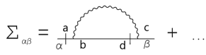
Figure 2: Diagrammatic representation for $\Sigma_{\alpha\beta}$.

Here the ellipsis stands for the 2-, 3- and other N-loop diagrams.

The typical feature of all rapid-change models like (1) with retarded bare propagator of the type (17) is that all the skeleton multiloop diagrams entering into the self-energy operator contain closed circuits of such retarded propagators and therefore vanish RG ; AntGul2012-mod ; VectorN . The dependence of the frequency in function $D_{v}$ [see (10)] destroys this easy construction, and now all the N-loop diagrams are expected to give some nontrivial contribution to the function $\Sigma_{\alpha\beta}$.

Let us start with the one-loop diagram. It is represented by the expression

$$\Sigma_{\alpha\beta}=D_{0}\int\frac{d\omega}{2\pi}\int\frac{d{\bf k}}{(2\pi)^{d}}\frac{2\pi\,\delta(k_{\parallel})k_{\perp}^{5-d-(\xi+\eta)}}{\left(-i\omega+\nu_{0}\left[\left({\bf p+k}\right)_{\perp}^{2}+f_{0}\left(p+k\right)_{\parallel}^{2}\right]\right)\left(\omega^{2}+\left[\alpha_{0}\nu_{0}k_{\perp}^{2-\eta}\right]^{2}\right)}P_{\alpha i}({\bf p})J_{ij}P_{j\beta}({\bf p}),$$ (29)

where the fraction is a product of the propagator function (17) and the correlator (10), transverse projectors $P_{\alpha i}({\bf p})$ and $P_{\beta j}({\bf p})$ are present due to the transversality conditions (20), and $J_{ij}$ is an index structure of this diagram:

$$J_{ij}=V_{i\,ab}({\bf p})V_{d\,cj}({\bf p+k})P_{bd}({\bf p+k})n_{a}n_{c}.$$ (30)

Here and below $V_{ijk}({\bf p})$ is the triple vertex (16); the Greek letters $\alpha$, $\beta$ and the Roman letters $a$–$d$ denote the vector indices of the propagators (8) and (17) with the implied summation over repeated indices. Since the index of divergence for this diagram $d_{\Gamma}=2$, we need to calculate only the terms, proportional to ${\bf p}^{2}$.

The calculation of this diagram is similar to the zero-time correlation case VectorN , so we will discuss it here only briefly.

The integration over the frequency $\omega$ is trivial. In order to integrate over the vector ${\bf k}$ with the function $\delta(k_{\parallel})$ in the integrand we need to average the expression (29) over the angles:

$$\int d{\bf k}\,\delta(k_{\parallel})f({\bf k})=S_{d-1}\int_{m}^{\infty}dk_{\perp}\,k_{\perp}^{d-2}\,\left\langle f({\bf k}_{\perp})\right\rangle,$$ (31)

where $\langle\cdots\rangle$ is the averaging over the unit sphere in the $(d-1)$-dimensional space, $S_{d-1}$ is its surface area, and $k_{\perp}=|{\bf k}_{\perp}|$. To average some function of $k_{\perp}$ over the angles in the orthogonal subspace we use the following expression:

$$\left\langle\frac{k_{i}^{\perp}k_{j}^{\perp}}{k_{\perp}^{2}}\right\rangle=\frac{P_{ij}({\bf n})}{(d-1)}.$$ (32)

This gives:

$$\Sigma_{\alpha\beta}=-\frac{g_{0}\nu_{0}f_{0}}{2\alpha_{0}}C_{d-1}\left[\frac{d-2+{\cal A}_{0}}{d-1}P_{\alpha\beta}({\bf p})+\frac{({\cal A}_{0}-1)^{2}}{d-1}\hat{n}_{\alpha}\hat{n}_{\beta}\right]({\bf pn})^{2}\int_{m}^{\infty}dk_{\perp}\frac{k_{\perp}^{1-\xi}}{k_{\perp}^{2}+\alpha_{0}k_{\perp}^{2-\eta}},$$ (33)

where $C_{d-1}\equiv S_{d-1}/(2\pi)^{d-1}$ and the vector $\hat{n}_{k}$, which is orthogonal to ${\bf p}$, is defined as

$$\hat{n}_{k}=P_{mk}({\bf p})n_{m}=n_{k}-p_{\parallel}p_{k}/p^{2}.$$ (34)

The integral over $k_{\perp}$ in expression (33) can be simplified in the minimal subtraction (MS) renormalization scheme, which we adopt in what follows. In that scheme, all the anomalous dimensions $\gamma$ are independent of the regularizators like $\xi$ and $\eta$, and we may chose them arbitrary with the only restriction – our diagrams have to remain UV finite; see FinTimeEta for detailed discussion. The most convenient way is to put $\eta=0$, so the expression (33) turns into

$$\Sigma_{\alpha\beta}=-\frac{g_{0}\nu_{0}f_{0}}{2\alpha_{0}(1+\alpha_{0})}C_{d-1}\left[\frac{d-2+{\cal A}_{0}}{d-1}P_{\alpha\beta}({\bf p})+\frac{({\cal A}_{0}-1)^{2}}{d-1}\hat{n}_{\alpha}\hat{n}_{\beta}\right]({\bf pn})^{2}\int_{m}^{\infty}dk_{\perp}\frac{1}{k_{\perp}^{1+\xi}}$$ (35)

and we obtain the following result:

$$\Sigma_{\alpha\beta}=-\frac{g_{0}\nu_{0}f_{0}}{2\alpha_{0}(1+\alpha_{0})}C_{d-1}\left[\frac{d-2+{\cal A}_{0}}{d-1}P_{\alpha\beta}({\bf p})+\frac{({\cal A}_{0}-1)^{2}}{d-1}\hat{n}_{\alpha}\hat{n}_{\beta}\right]({\bf p\cdot n})^{2}\frac{m^{-\xi}}{\xi}.$$ (36)

The remaining multiloop diagrams will be discussed a bit later, in section IV.3.

IV.2 Perturbation expansion for the 1-irreducible function $\langle\theta^{\prime}_{\alpha}\theta_{\beta}v_{\gamma}\rangle_{\text{1-ir}}$

The expansion like (28) for the function $\langle\theta^{\prime}_{\alpha}\theta_{\beta}v_{\gamma}\rangle_{\text{1-ir}}$ has the form

$$\langle\theta^{\prime}_{\alpha}\theta_{\beta}v_{\gamma}\rangle_{\text{1-ir}} = V_{\alpha\,\beta\gamma}+\Delta_{\alpha\,\beta\gamma}$$ (37)

$$= i\delta_{\alpha\gamma}p_{\beta}-i{\cal A}_{0}\delta_{\alpha\beta}p_{\gamma}+\Delta_{\alpha\,\beta\gamma},$$

where $V_{\alpha\,\beta\gamma}$ is the vertex (16) and $\Delta_{\alpha\,\beta\gamma}$ is represented in the Fig. 3.

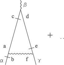
Figure 3: Diagrammatic representation for $\Delta_{\alpha\,\beta\gamma}$.

As in the case of self energy operator in Fig. 2, the ellipsis stands for the 2-, 3- and other N-loop diagrams.

Since our model is Galilean invariant, as discussed in Sec. II, the terms $\theta^{\prime}_{k}\partial_{t}\theta_{k}$ and $\theta^{\prime}_{k}(v_{i}\partial_{i})\theta_{k}$ in the action functional may be renormalized only with the only renormalization constant $Z_{1}$. The index of divergence for this function is $d_{\Gamma}=1$, so that the counterterms with $\partial_{t}$ are forbidden. Consequently, counterterm $\theta^{\prime}_{k}(v_{i}\partial_{i})\theta_{k}$ is also forbidden. If ${\cal A}_{0}=1$, the vertex (16) is transverse, the nonlocal term $\partial{\cal P}$ in the stochastic equation (4) is absent and the action functional is local in-time. This means that the counterterm $\theta^{\prime}_{k}(\theta_{i}\partial_{i})v_{k}$ is forbidden because the appearance of some constant $Z_{2}$, which this term is renormalized by, is equivalent to appearance of some multiplier like ${\cal A}_{0}\neq 1$, i.e., the appearance of nonlocal terms in the action functional. Similar reasoning exclude the appearance of such a counterterm if ${\cal A}_{0}=0$. Thus, we may conclude, that $\Delta_{\alpha\beta\gamma}$ is proportional to ${\cal A}_{0}({\cal A}_{0}-1)$ and vanish for the aforementioned cases.

The procedure of calculating the one-loop approximation of $\Delta_{\alpha\,\beta\gamma}$ is similar to the one-loop contribution to the self-energy operator $\Sigma_{\alpha\beta}$, discussed in previous section. The analytical expression for the former is

$$\Delta_{\alpha\beta\gamma}=D_{0}\int\frac{d\omega}{2\pi}\int\frac{d{\bf k}}{(2\pi)^{d}}\frac{1}{\left(-i\omega+\nu_{0}\left[({\bf k+q})_{\perp}^{2}+f_{0}(k+q)_{\parallel}^{2}\right]\right)\left(-i\omega+\nu_{0}\left[({\bf k-p})_{\perp}^{2}+f_{0}(k-p)_{\parallel}^{2}\right]\right)}\noindent$$

$$\times\frac{2\pi\,\delta(k_{\parallel})k_{\perp}^{5-d-(\xi+\eta)}}{\left(\omega^{2}+\left[\alpha_{0}\nu_{0}k_{\perp}^{2-\eta}\right]^{2}\right)}P_{\alpha i}({\bf q})J_{i\beta j}P_{j\gamma}({\bf p})n_{\beta},$$ (38)

where ${\bf p}$ and ${\bf q}$ are two external momenta, $J_{i\beta j}$ is the index structure of this diagram, transverse projectors $P_{i\alpha}({\bf p})$ and $P_{j\gamma}({\bf p})$ and vector $n_{\beta}$ are present due to the transversality conditions (20) and definition (3). Since the index of divergence for this function is $d_{\Gamma}=1$, we need to calculate only the term, proportional to the linear combination of ${\bf p}$ and ${\bf q}$. Also we may put $\eta=0$ in this diagram and left with the only regularizator $\xi$.

The integral over $\omega$ is convergent; direct calculation shows that

$$J_{i\beta j}\propto{\cal A}_{0}(1-{\cal A}_{0})n_{i}P_{\beta j}({\bf n}).$$ (39)

This means that

$$J_{\alpha\beta\gamma}\equiv P_{\alpha i}({\bf q})J_{i\beta j}P_{j\gamma}({\bf p})n_{\beta}=0,$$ (40)

i.e., the function $\langle\theta^{\prime}_{\alpha}\theta_{\beta}v_{\gamma}\rangle_{\text{1-ir}}$ does not diverge not only for the cases ${\cal A}_{0}=0$ and ${\cal A}_{0}=1$, discussed above, but also in all the other situations.

The multiloop diagrams will be discussed in the next subsection.

IV.3 Multiloop diagrams

In order to renormalize our model we have to deal with two types of multiloop diagrams – one of types corresponds to the function $\langle\theta_{\alpha}^{\prime}\theta_{\beta}\rangle_{\rm 1-ir}$ and is represented in Fig. 2, the other one corresponds to the function $\langle\theta^{\prime}_{\alpha}\theta_{\beta}v_{\gamma}\rangle_{\text{1-ir}}$ and is represented in Fig. 3. Let us start with the latter. Any multiloop diagram of this type contains a part with the structure, represented in Fig. 4.

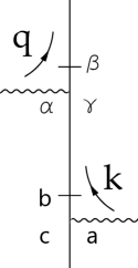
Figure 4: Fragment of arbitrary multiloop diagram, entering into expansion of the function $\langle\theta^{\prime}_{\alpha}\theta_{\beta}v_{\gamma}\rangle_{\text{1-ir}}$.

Since it is sufficient to calculate all the diagrams at external momenta equal to zero (the real index of divergence $d_{\Gamma}^{\prime}=0$), the integral, corresponding to the divergent part of the diagram, necessarily contains as a factor the following expression:

$$I_{0}\propto\delta(k_{\parallel})\delta(q_{\parallel})n_{a}V_{bac}({\bf k})n_{\alpha}V_{\beta\alpha\gamma}({\bf k+q})P_{\gamma b}({\bf k}),$$ (41)

where $V$ is the vertex (16), and the $\delta$-functions appear from velocity correlator (8). Since $I_{0}$ is proportional to the sum of $k_{\parallel}$ and $q_{\parallel}$ with some coefficients, after integration with the $\delta$-functions all these diagrams vanish.

Any multilop diagram, entering into the expansion of the 1-irreducible linear response function $\langle\theta_{\alpha}^{\prime}\theta_{\beta}\rangle_{\rm 1-ir}$, contains a part with structure, represented in Fig. 5 or a part with structure, represented in Fig. 6.

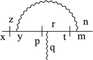
Figure 5: One of two possible fragments of arbitrary multiloop diagram for self-energy operator $\Sigma_{\alpha\beta}$.

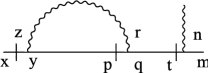
Figure 6: Another possible fragment of arbitrary multiloop diagram for self-energy operator $\Sigma_{\alpha\beta}$.

Since in any 1-irreducible diagram it is always possible to move the derivative onto external “tail” $\theta^{\prime}_{k}$, the real index of divergence for this diagram $d_{\Gamma}^{\prime}=1$. This means, that in course of calculation of the structures, represented in Fig. 5 and Fig. 6, we are interested only in terms, linear in the external momenta ${\bf p}$.

The analytical expression for the first structure, denoted by $I_{1}$, is proportional to

$$I_{1} \propto \delta(k_{\parallel})\delta(q_{\parallel})n_{z}V_{xyz}({\bf p+k})P_{yp}({\bf p+k-q})$$

$$\times n_{q}V_{pqr}({\bf p+k-q})P_{rt}({\bf p-q})n_{n}V_{tnm}({\bf p-q}).$$

Here ${\bf p}$ is the external momentum, ${\bf k}$ and ${\bf q}$ are internal integration momenta, $V$ is the vertex (16), $P$ is the transverse projector, and the unit vector ${\bf n}$ and $\delta$-functions stem from velocity correlator (8).

Direct calculation shows, that $I_{1}$ is proportional to some linear combination of $k_{\parallel}$ and $q_{\parallel}$, and, as well as in the case of $I_{0}$, after the integration with the $\delta$-functions all diagrams with this structure vanish.

Another structure, represented in Fig. 6, possess the same property – analytical expression for it is similar to (IV.3), and, as can be seen from the direct calculation, all the diagrams with this structure also appear to be equal to zero.

It should be stressed that, in contrast to rapid-change models like (1) with $\delta$ functions in time, where all these multiloop diagrams vanish due to the closed circuits of retarded propagators, in our model their vanishing has a rather nontrivial origin and results from the presence of the anisotropy in it.

IV.4 Renormalization and RG equations

Substitution of the explicit expression (36) for the divergent part of the self-energy operator $\Sigma_{\alpha\beta}$ into the expression (28) for the 1-irreducible linear response function $\Gamma_{2}^{\alpha\beta}$ gives

$$\Gamma_{2}^{\alpha\beta}=\{i\omega-\nu_{0}{\bf p}_{\perp}^{2}-\nu_{0}f_{0}({\bf p\cdot n})^{2}\}\ P_{\alpha\beta}({\bf p})-\frac{g_{0}\nu_{0}f_{0}}{2\alpha_{0}(1+\alpha_{0})}\left[\frac{(d-2+{\cal A}_{0})}{d-1}P_{\alpha\beta}({\bf p})+\frac{({\cal A}_{0}-1)^{2}}{d-1}\hat{n}_{\alpha}\hat{n}_{\beta}\right]C_{d-1}({\bf p\cdot n})^{2}\times\frac{m^{-\xi}}{\xi}.$$ (43)

The renormalization constants are found from the requirement that the function (43), when expressed in new renormalized variables, be UV finite, i.e., finite at $\xi\to 0$. From the analysis of this expression it follows, however, that the pole in $\xi$ in the structure with $\hat{n}_{\alpha}\hat{n}_{\beta}$ cannot be removed by renormalization of the model parameters because the bare part of $\Gamma_{2}^{\alpha\beta}$ does not contain analogous term. In order to ensure multiplicative renormalizability one has to add such term, with a new positive amplitude factor $u_{0}$, to the bare part:

$$\Gamma_{2}^{\alpha\beta} = \left\{i\omega-\nu_{0}{\bf p}_{\perp}^{2}-\nu_{0}f_{0}({\bf p\cdot n})^{2}\right\}\ P_{\alpha\beta}({\bf p})-\nu_{0}f_{0}u_{0}\ ({\bf p\cdot n})^{2}\hat{n}_{\alpha}\hat{n}_{\beta}$$ (44)

$$- \frac{g_{0}\nu_{0}f_{0}}{2\alpha_{0}(1+\alpha_{0})}\left[\frac{(d-2+{\cal A}_{0})}{d-1}P_{\alpha\beta}({\bf p})+\frac{({\cal A}_{0}-1)^{2}}{d-1}\hat{n}_{\alpha}\hat{n}_{\beta}\right]C_{d-1}({\bf p\cdot n})^{2}\times\frac{m^{-\xi}}{\xi}.$$

This means that the original model (12) is extended by adding a new term of the form $u_{0}f_{0}\nu_{0}(n_{k}\theta_{k}^{\prime})\partial_{\parallel}^{2}(n_{k}\theta_{k})$; the interpretation of the new parameter $u_{0}$ is literally the same as for $f_{0}$ in Sec. II.

Now the model is multiplicatively renormalizable with two independent renormalization constants $Z_{f}$ and $Z_{u}$:

$$\nu_{0}=\nu Z_{\nu},\ f_{0}=fZ_{f},\ u_{0}=uZ_{u},\$$

$${\cal A}_{0}={\cal A}Z_{\cal A},\ g_{0}=g\mu^{\xi+\eta}Z_{g},\ \alpha_{0}=\alpha\mu^{\eta}Z_{\alpha},$$ (45)

at that

$$Z_{\nu}=Z_{\alpha}=Z_{\cal A}=1,\ Z_{g}=Z_{f}^{-1}.$$ (46)

Here $\mu$ is the “reference mass” (additional free parameter of the renormalized theory) in the MS renormalization scheme, which we always use in what follows; $g$, $u$, $\alpha$, $\nu$, ${\cal A}$ and $f$ are renormalized analogs of the bare parameters $g_{0}$, $u_{0}$, $\alpha_{0}$, $\nu_{0}$, ${\cal A}_{0}$ and $f_{0}$, and $Z_{i}=Z_{i}(g,\xi,d)$ are the renormalization constants. Their relations in (46) result from the absence of renormalization of the contribution with $D_{v}^{-1}$ in (12), so that $D_{0}\equiv g_{0}\nu_{0}^{3}f_{0}=g\mu^{\xi+\eta}\nu^{3}f$, $\alpha_{0}\nu_{0}=\alpha\mu^{\eta}\nu$. No renormalization of the fields and the parameter $m_{0}=m$ is needed: i.e., $Z_{\Phi}=1$ for all $\Phi$ and $Z_{m}=1$.

The renormalized action functional has the form

$${\cal S}_{R}(\Phi) = \frac{1}{2}\theta^{\prime}_{i}D_{\theta}\theta^{\prime}_{k}-\frac{1}{2}v_{i}D_{v}^{-1}v_{k}+\theta^{\prime}_{k}\left[-\partial_{t}\theta_{k}-(v_{i}\partial_{i})\theta_{k}+{\cal A}(\theta_{i}\partial_{i})v_{k}+\nu(\partial_{\perp}^{2}+fZ_{f}\partial_{\parallel}^{2})\theta_{k}\right]+$$ (47)

$$+ \nu\,fZ_{f}\,uZ_{u}\,(n_{k}\theta_{k}^{\prime})\partial_{\parallel}^{2}(n_{k}\theta_{k}),$$

where the function $D_{v}$ from (10) should be expressed in renormalized variables using (IV.4).

At this moment one important problem springs up. Since the original model is extended by introducing a new term (proportional to the $\theta^{\prime}_{i}\theta_{k}$) in the action functional (12), one may guess that the propagator functions (17) and (18) have to be modified. Consequently, we have to recalculate the diagrams for functions $\langle\theta_{\alpha}^{\prime}\theta_{\beta}\rangle_{\rm 1-ir}$ and $\langle\theta^{\prime}_{\alpha}\theta_{\beta}v_{\gamma}\rangle_{\text{1-ir}}$, i.e., the expressions (36) and (40).

If fact, the difference between the original expressions for the bare propagators and the new ones is that the second have additional terms, which are proportional to the $p_{\parallel}$. Consequently, they do not contribute to the integrals and revision of the final expressions is in fact not needed; this means that expressions (36) and (40) remain valid in the modified model. This problem was examined in details in VectorN ; moreover, the derivation of the propagators in the presence of a distinguished direction ${\bf n}$, i.e., in fact, the matrix inversion in the orthogonal subspace, was also discussed there.

Now we are ready to study the fixed points $\left\{g_{i}^{*}\right\}$ that govern the IR asymptotic behavior. The basic RG equation for a multiplicatively renormalizable quantity (correlation function, composite operator, etc.) has the form

$$\bigl{[}{\cal D}_{RG}+\gamma_{F}\bigr{]}F_{R}=0$$ (48)

and is a consequence of operating on the relation $F=Z_{F}F_{R}$ with the differential operation $\mu\partial_{\mu}$ for fixed set of bare parameters $e_{0}$ $=$ $\left\{g_{0},\nu_{0},f_{0},u_{0},{\cal A}_{0}\right\}$. This operation is customarily denoted as $\widetilde{\cal D}_{\mu}$, and $\gamma_{F}$ is the anomalous dimension of $F$. Since $Z_{\nu}=1$, the renormalization group operator ${\cal D}_{RG}$ has the form ${\cal D}_{RG}={\cal D}_{\mu}+\beta_{g}\partial_{g}-\gamma_{f}{\cal D}_{f}-\gamma_{u}{\cal D}_{u}$, where ${\cal D}_{x}\equiv x\partial_{x}$ for any variable $x$.

The RG functions are defined as

$$\beta_{g}\equiv\widetilde{\cal D}_{\mu}g=g\,[-\xi-\eta-\gamma_{g}(g)],$$ (49a)

$$\beta_{u}\equiv\widetilde{\cal D}_{\mu}u=-u\gamma_{u}(g,u),$$ (49b)

$$\beta_{\alpha}\equiv\widetilde{\cal D}_{\mu}\alpha=-\eta\alpha,$$ (49c)

$$\gamma_{F}\equiv\widetilde{\cal D}_{\mu}\ln Z_{F}=\beta_{g}\partial_{g}\ln Z_{F}\quad{\rm for\ any\ }Z_{F}.$$ (49d)

The relations between $\beta$ and $\gamma$ in (49a) – (49c) result from their definitions along with relations (IV.4) and (46).

The constants $Z_{i}$ are found from the requirement of UV finiteness of the expression (44). Thus, for the parameter $f_{0}$ that splits the Laplace operator we obtain

$$Z_{f}=1-\frac{(d-2+{\cal A})}{2(d-1)}\ \frac{g}{\alpha(\alpha+1)}\frac{1}{\xi}+O\left(g^{2}\right),$$ (50)

$$\gamma_{f}=\frac{\left(d-2+{\cal A}\right)}{2(d-1)}\ \frac{g}{\alpha(\alpha+1)},$$ (51)

where we passed to the new coupling constant $g\equiv\tilde{g}\,C_{d-1}$ with $C_{d-1}$ from (36).

Then we have to renormalize the constant $u_{0}$ such that the expression

$$g_{0}f_{0}u_{0}\left[1+\frac{({\cal A}-1)^{2}}{2(d-1)}\frac{1}{u_{0}\,\alpha_{0}(1+\alpha_{0})}\times\frac{m^{-\xi}}{\xi}\right]n_{\alpha}n_{\beta}({\bf p\cdot n})^{2}$$ (52)

be UV finite to the first order in $g$. Therefore,

$$Z_{u}Z_{f}=1-\frac{({\cal A}-1)^{2}}{2(d-1)}\ \frac{g}{u\,\alpha(1+\alpha)}\ \frac{1}{\xi}+O\left(g^{2}\right),$$ (53)

and

$$\gamma_{u}+\gamma_{f}=\frac{({\cal A}-1)^{2}}{2(d-1)}\ \frac{g}{u\,\alpha(1+\alpha)},$$ (54)

where the constant $\gamma_{f}$ is obtained in (51). Furthermore, from the last relation in (46) it follows that for the coupling constant $g$

$$\gamma_{g}=-\gamma_{f}=-\frac{(d-2+{\cal A})}{2(d-1)}\ \frac{g}{\alpha(1+\alpha)}.$$ (55)

We stress that, since the expression (44) is exact, i.e., it has no corrections in coupling constant $g$, all the above expressions for the anomalous dimensions $\gamma_{f,g,u}$ are exact, too.

IV.5 Fixed points

One of the basic RG statements is that the asymptotic behavior of the model is governed by the fixed points $\left\{g^{*},\alpha^{*},u^{*},f^{*}\right\}$, defined by the relations

$$\beta_{g}=0,\quad\beta_{u}=0,\quad\beta_{f}=0\quad\text{and}\quad\beta_{\alpha}=0;$$ (56)

here

$$\beta_{g}=g\left(-\xi-\eta+\gamma_{f}\right)=g\left[-\xi-\eta+\frac{(d-2+{\cal A})}{2(d-1)}\ \frac{g}{\alpha(1+\alpha)}\right],$$ (57a)

$$\beta_{u}=-u\gamma_{u}=\frac{g}{\alpha(\alpha+1)}\left[\frac{(d-2+{\cal A})}{2(d-1)}u-\frac{({\cal A}-1)^{2}}{2(d-1)}\right],$$ (57b)

$$\beta_{f}=-f\gamma_{f}=-f\frac{(d-2+{\cal A})}{2(d-1)}\ \frac{g}{\alpha(1+\alpha)},$$ (57c)

the expression for $\beta_{\alpha}$ is written in (49c).

The type of a fixed point (IR/UV attractive or a saddle point), i.e., the character of the RG flow in vicinity of the point, is determined by the matrix $\Omega_{ik}=\partial\beta_{i}/\partial g_{k}$, where $\beta_{i}$ is the full set of $\beta$-functions and $g_{k}$ is the full set of couplings. For an IR attractive fixed point the matrix $\Omega$ are positive, i.e., the real parts of all its eigenvalues are positive.

The analysis of the $\beta$-functions reveals several fixed points. The first possibility is to put $\alpha^{*}=0$; consequently we get at once the trivial case $g^{*}=0$. There is, however, another possibility – to disclose it we have to pass from the coupling constant $g$ to new constant $g^{\prime}=g/\alpha$, which is assumed to be finite at $\alpha\to 0$. In fact this means, that the correlation function $D_{v}(\omega)$ becomes proportional to $\delta(\omega)$ (see (10)) and we deal with the independent of time (“frozen” or “quenched”) velocity field.

The new $\beta$-function, which remains nonzero at $\alpha\to 0$, is

$$\beta_{g^{\prime}}=\frac{1}{\alpha}\beta_{g}-\frac{g}{\alpha^{2}}\beta_{\alpha}=g^{\prime}\left[-\xi+\frac{(d-2+{\cal A})}{2(d-1)}g^{\prime}\right];$$ (58)

the matrix $\Omega$ in these variables has the form

$$\Omega=\begin{pmatrix}\partial_{g^{\prime}}\beta_{g^{\prime}}&\partial_{g^{\prime}}\beta_{u}&0&\partial_{g^{\prime}}\beta_{f}\\ 0&\partial_{u}\beta_{u}&0&0\\ 0&0&\partial_{\alpha}\beta_{\alpha}&0\\ 0&0&0&\partial_{f}\beta_{f}\\ \end{pmatrix}.$$ (59)

This situation implies two options:

(1a) $g^{\prime*}=0$, with $\Omega_{g^{\prime}g^{\prime}}^{*}=\left.\partial\beta_{g^{\prime}}/\partial g^{\prime}\right|_{g^{\prime}=g^{\prime*}}=-\xi$ and $\Omega_{\alpha\alpha}^{*}=-\eta$.

For the two remaining parameters $u$ and $f$ we have $\beta_{u}=\beta_{f}\equiv 0$, $\Omega_{uu}^{*}=\Omega_{ff}^{*}\equiv 0$, so that both $u$ and $f$ remain free parameters.

Since $\Omega_{g^{\prime}u}^{*}=0$, the matrix $\Omega$ is triangle and its eigenvalues coincide with the diagonal elements. Thus, this fixed point is IR attractive for $\xi<0$, $\eta<0$;

(1b) if $g^{\prime*}=\xi\frac{2(d-1)}{d-2+{\cal A}}$, $\Omega_{g^{\prime}g^{\prime}}^{*}=\xi$ and $\Omega_{\alpha\alpha}^{*}=-\eta$, so that this fixed point is IR attractive for $\xi>0$, $\eta<0$. For the remaining parameters $u$ and $f$ we have the fixed-point values $u^{*}=({\cal A}-1)^{2}/(d-2+{\cal A})$ and $f^{*}=\infty$ with $\Omega_{uu}^{*}=\Omega_{ff}^{*}=\xi$.

Another interesting case to be considered is $\alpha^{*}=\infty$. From (10) it follows that this case corresponds to the rapid-change model with new charge $g^{\prime\prime}=g/\alpha^{2}$, which is supposed to be finite at $\alpha\to\infty$. Besides that it is convenient to pass from the variable $\alpha$ to variable $x=1/\alpha$, i.e., $x\to 0$. So, the new $\beta$-functions are

$$\beta_{x}=x\eta;$$ (60a)

$$\beta_{u}=g^{\prime\prime}\left[\frac{(d-2+{\cal A})}{2(d-1)}u-\frac{({\cal A}-1)^{2}}{2(d-1)}\right];$$ (60b)

$$\beta_{f}=g^{\prime\prime}\left[-f\frac{(d-2+{\cal A})}{2(d-1)}\right];$$ (60c)

$$\beta_{g^{\prime\prime}}=\frac{1}{\alpha^{2}}\beta_{g}-\frac{2g}{\alpha^{3}}\beta_{\alpha}=g^{\prime\prime}\left[-\xi+\eta+\frac{(d-2+{\cal A})}{2(d-1)}g^{\prime\prime}\right].$$ (60d)

Thus, we find two more fixed points:

(2a) $g^{\prime\prime*}=0$, with $\Omega_{g^{\prime\prime}g^{\prime\prime}}^{*}=-\xi+\eta$, $\Omega_{xx}^{*}=\eta$. As in the case (1a) for two remaining parameters $u$ and $f$ we have $\beta_{u}=\beta_{f}\equiv 0$, $\Omega_{uu}^{*}=\Omega_{ff}^{*}\equiv 0$, so both of them remain free parameters.

As before the matrix $\Omega$ in the new variables $\left\{g^{\prime\prime},x,u,f\right\}$ is a matrix of the type (59), i.e., it is triangle and its eigenvalues are simply given by diagonal elements. Thus, this fixed point is IR attractive for $\eta>0$, $\eta-\xi>0$;

(2b) if $g^{\prime\prime*}=(\xi-\eta)\frac{2(d-1)}{d-2+{\cal A}}$, $\Omega_{g^{\prime\prime}g^{\prime\prime}}^{*}=\xi-\eta$ and $\Omega_{xx}^{*}=\eta$, so that this fixed point is IR attractive for $\eta>0$, $\xi-\eta>0$. For the remaining parameters $u$ and $f$ we have the fixed-point values $u^{*}=({\cal A}-1)^{2}/(d-2+{\cal A})$ and $f^{*}=\infty$ with $\Omega_{uu}^{*}=\Omega_{ff}^{*}=\xi-\eta$.

For the special case $\eta=0$ the function $\beta_{\alpha}$ and the eigenvalue $\Omega_{\alpha\alpha}$ vanish identically, so that the nontrivial fixed point $\left[g/\alpha(\alpha+1)\right]^{*}=2\xi(d-1)/(d-2+{\cal A})$ is IR attractive for $\xi>0$. Moreover, this fixed point is degenerate in the sense that we can not determine the parameters $g^{*}$ and $\alpha^{*}$ separately.

Thus, we can conclude, that the domains of IR stability in this vector model (12) coincide with the corresponding domains of IR stability in scalar model, considered in AntMal2011 . The general pattern of the fixed points stability in the $\xi$ — $\eta$ plane is shown in Fig. 7. The straight lines $\eta=0$; $\xi=0$, $\eta<0$; and $\xi=\eta$, $\eta>0$ corresponds to the boundaries of domains, which has neither gaps nor overlaps between them. Since the $\beta$-functions (57) have no higher-order corrections, this pattern is exact.

Note that the Kolmogorov values of the exponents $\xi=8/3$, $\eta=4/3$ lie deep inside the domain of stability of the nontrivial rapid-change point (2b); there is no borderline going through this point.

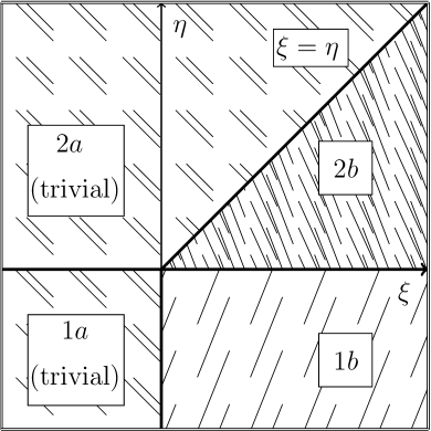
Figure 7: Domains of IR stability of the fixed points in the model (12). The numbers in boxes correspond to the fixed points (1a) – (2b) in the text.

This fact implies that the correlation functions of the model (12) in the IR region ($\mu r\simeq\Lambda r\gg 1$, $Mr\sim 1$) exhibit scaling behavior (as we will see below, up to logarithmic factors).

The corresponding critical dimensions $\Delta[F]\equiv\Delta_{F}$ for all basic fields and parameters can be calculated exactly; see the next subsection.

IV.6 Critical dimensions

In the leading order of the IR asymptotic behavior the Green functions satisfy the RG equation (48) with the substitution $g\to g^{*}$, $\alpha\to\alpha^{*}$, $f\to f^{*}$ and $u\to u^{*}$. The operator ${\cal D}_{RG}$ is invariant with respect to the change of variables $\left\{x,y\right\}\to\left\{x^{\prime},y^{\prime}\right\}$, i.e., $\beta_{x}\partial_{x}+\beta_{y}\partial_{y}=\beta_{x^{\prime}}\partial_{x^{\prime}}+\beta_{y^{\prime}}\partial_{y^{\prime}}$. Taking into account the fact that $\gamma_{u}^{*}=0$, this gives

$$\left[{\cal D}_{\mu}-\gamma_{f}^{*}{\cal D}_{f}+\gamma_{G}^{*}\right]\,G^{R}(e,\mu,\dots)=0.$$ (61)

Canonical scale invariance is expressed by the relations

$$\left[\sum_{\sigma}d_{\sigma}^{k}{\cal D}_{\sigma}-d_{G}^{k}\right]G^{R}=0,\quad\left[\sum_{\sigma}d_{\sigma}^{\omega}{\cal D}_{\sigma}-d_{G}^{\omega}\right]G^{R}=0,$$ (62)

where $\sigma\equiv\{t,{\bf x},\mu,\nu,\alpha,m,M,u,f,{\cal A},g\}$ is the set of all arguments of $G^{R}$ ($t,{\bf x}$ is the set of all times and coordinates), and $d^{k}$ and $d^{\omega}$ are the canonical dimensions of $G^{R}$ and $\sigma$. Substitution of the needed dimensions from Table 1 and combination of the obtained result with (61) gives the desired equation of critical IR scaling for the model:

$$\left[-{\cal D}_{\bf x}+\Delta_{t}{\cal D}_{t}+\Delta_{m}{\cal D}_{m}+\Delta_{M}{\cal D}_{M}+\Delta_{f}{\cal D}_{f}-\Delta_{G}\right]G^{R}=0,$$ (63)

where

$$\Delta_{t}=-\Delta_{\omega}=-2,\quad\Delta_{m}=\Delta_{M}=1,$$

$$\Delta_{f}=\gamma_{f}^{*},\quad\Delta_{u}=0$$ (64)

and

$$\Delta[G]\equiv\Delta_{G}=d_{G}^{k}+2d_{G}^{\omega}+\gamma_{G}^{*}$$ (65)

are the corresponding critical dimensions. Substituting the values of fixed point of the regimes (1a)–(2b) we obtain:

$$\Delta_{f}=0\quad\text{for (1a), (2a)};$$ (66)

$$\Delta_{f}=\xi\quad\text{for (1b)}, \Delta_{f}=\xi-\eta\quad\text{for (2b)}.$$ and

In particular, for any correlation function $G^{R}=\langle\Phi\dots\Phi\rangle$ of the fields $\Phi$ we have $\Delta_{G}=N_{\Phi}\Delta_{\Phi}$, with the summation over all fields $\Phi$ entering into $G^{R}$, namely,

$$\Delta_{G}=\sum_{\Phi}N_{\Phi}d_{\Phi}=N_{\theta^{\prime}}d_{\theta^{\prime}}+N_{\theta}d_{\theta}+N_{v}d_{v}.$$ (67)

Since in the model (12) the fields themselves are not renormalized (i.e., $\gamma_{\Phi}=0$ for all $\Phi$, see sec. IV.4), using (65) we conclude, that the critical dimensions of the fields $\Phi=\left\{\bm{v},{\bm{\theta}},{\bm{\theta}^{\prime}}\right\}$ are the same as their canonical dimensions, presented in the Table 1. Namely,

$$\Delta_{\bm{v}}=1,\quad\Delta_{\theta}=-1,\quad\Delta_{\theta^{\prime}}=d+1.$$ (68)

It is the specific feature of the present model, which makes it similar to the zero-correlation time model VectorN and distinguishes it from both the isotropic Kraichnan’s vector model AntGul2012-mod (in which $\gamma_{\nu}\neq 0$) and anisotropic Kraichnan’s scalar model AntMal2011 (in which the Laplacian splitting parameter $f_{0}$ is not dimensionless).

V Renormalization and critical dimensions of composite operators

The analysis of the renormalization of composite operators is nearly the same as in the rapid-change model VectorN , so we will discuss it here very briefly.

V.1 General scheme

The central role in the following will be played by composite fields (“operators”) built solely of the basic fields $\theta$:

$$F_{Np}=(\theta_{i}\theta_{i})^{p}\ (n_{s}\theta_{s})^{2m},$$ (69)

where $N=2(p+m)$ is the total number of fields $\theta$, entering the operator.

As was pointed out in VectorN , the operator counterterms to a certain $F_{Np}$ involve only operators of the form (69) with the same value of $N$. Besides that, all the corresponding diagrams diverge logarithmically and one can calculate them with all external frequencies and momenta set equal to zero.

Let us denote the closed set of operators, which can mix to each other in renormalization, as $F\equiv\{F_{Np}\}$. The renormalization matrix $\hat{Z}_{F}\equiv\{Z_{Np,Np^{\prime}}\}$ for this set, given by the relation

$$F_{Np}=\sum_{p^{\prime}}Z_{Np,Np^{\prime}}F_{Np^{\prime}}^{R},$$ (70)

is determined by the requirement that the 1-irreducible correlation function

$$\bigl{\langle}F_{Np}^{R}(x)\theta(x_{1})\dots\theta(x_{N})\bigr{\rangle}_{\rm 1-ir}=$$

$$=\sum_{p^{\prime}}Z_{Np,\,Np^{\prime}}^{-1}\bigl{\langle}F_{Np^{\prime}}(x)\theta(x_{1})\dots\theta(x_{N})\bigr{\rangle}_{\rm 1-ir}\equiv\sum_{p^{\prime}}Z_{Np,\,Np^{\prime}}^{-1}\Gamma_{Np^{\prime}}(x;x_{1},\dots,x_{N})$$ (71)

be UV finite in renormalized theory, i.e., it has no poles in $\xi$ when expressed in renormalized variables (IV.4). This is equivalent to the UV finiteness of the sum $\sum_{p^{\prime}}Z_{Np,\,Np^{\prime}}^{-1}\Gamma_{Np^{\prime}}(x;\theta)$, in which

$$\Gamma_{Np^{\prime}}(x;\theta)=\frac{1}{N!}\,\int dx_{1}\dots\int dx_{N}\,\Gamma_{Np^{\prime}}(x;x_{1},\dots,x_{N})$$

$$\times\theta(x_{1})\dots\theta(x_{N})$$ (72)

is a functional of the field $\theta(x)$.

The contribution of a specific diagram into the functional $\Gamma_{Np^{\prime}}$ in (72) for any composite operator $F_{Np^{\prime}}$ is represented in the form

$$\Gamma_{Np^{\prime}}=V_{\alpha\beta\dots}\,I^{ab\dots}_{\alpha\beta\dots}\,\theta_{a}\theta_{b}\dots,$$ (73)

where $V_{\alpha\beta\dots}$ is the vertex factor, $I^{ab\dots}_{\alpha\beta\dots}$ is the “internal block” of the diagram with free vector indices, and the product $\theta_{a}\theta_{b}\dots$ corresponds to external “tails.”

According to the general rules of the universal diagrammatic technique (see, e.g., Vasiliev-Green ), for any composite operator $F(x)$ built of the fields $\theta$, the vertex $V_{\alpha\beta\dots}$ in (73) with $k\geq 0$ attached lines corresponds to the vertex factor

$$V^{k}_{Np}(x;\,x_{1},\dots,x_{k})\equiv\delta^{k}F_{Np}(x)/{\delta\theta(x_{1})\dots\delta\theta(x_{k})}.$$ (74)

The arguments $x_{1}\dots x_{k}$ of the quantity (74) are contracted with the arguments of the upper $\theta$ ends of the lines $\langle\theta\theta^{\prime}\rangle_{0}$ attached to the vertex.

V.2 Exact result for the diagrams

Now let us turn to the calculation of the internal block $I^{ab\dots}_{\alpha\beta\dots}$ of the diagrams. The one-loop diagram is represented in Fig. (8).

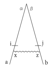
Figure 8: The one-loop contribution to the generating functional (72).

Once all the external frequencies and momenta are set to zero, the index structure of this diagram takes on the form

$$Y^{ab}_{\alpha\beta} = V_{xai}({\bf k})\ V_{zjb}({\bf-k})P_{\alpha i}({\bf k})P_{\beta j}({\bf k})n_{x}n_{z}$$ (75)

$$= -{\cal A}^{2}n_{x}P_{x\alpha}({\bf k})n_{z}P_{z\beta}({\bf k})\ k_{a}k_{b},$$

where the letters $i,j,x$ and $z$ denote internal indices of the diagram itself. Then we have to integrate $Y^{ab}_{\alpha\beta}$ over the frequency and momentum with the factors like (10) and (17), namely

$$I^{ab}_{\alpha\beta} = \int\frac{d{\bf k}}{(2\pi)^{d}}\frac{1}{-i\omega+\nu{\bf k}_{\perp}^{2}+\nu fk_{\parallel}^{2}}\frac{1}{i\omega+\nu{\bf k}_{\perp}^{2}+\nu fk_{\parallel}^{2}}$$ (76)

$$\times 2\pi\delta(k_{\parallel})\ D_{0}\ \frac{k_{\perp}^{5-d-(\xi+\eta)}}{\omega^{2}+\left[\alpha_{0}\nu_{0}k_{\perp}^{2-\eta}\right]^{2}}\ Y^{ab}_{\alpha\beta}.$$

Since the expression (76) contains the factor $\delta(k_{\parallel})$, we can perform all the calculations with the original propagators (17) and (18); see the discussion in Sec. IV.4.

Using the relation (32) for averaging over the angles and setting $\eta=0$ [see the discussion after (33)], we arrive at the following result:

$$I^{ab}_{\alpha\beta} = \frac{{\cal A}^{2}f}{2\alpha(1+\alpha)}g\int\frac{d{\bf k}_{\perp}}{(2\pi)^{d-1}}\ \frac{1}{k_{\perp}^{d-1+\xi}}\frac{k_{a}^{\perp}k_{b}^{\perp}}{k^{2}_{\perp}}\ n_{\alpha}n_{\beta}$$ (77)

$$= \frac{{\cal A}^{2}f}{2\alpha(\alpha+1)}\frac{1}{(d-1)}P_{ab}({\bf n})\ n_{\alpha}n_{\beta}\ g\times\frac{m^{-\xi}}{\xi}.$$

Contributions of all multiloop diagrams are equal to zero, see Sec. IV.3. The multiloop diagrams of the “sand clock” type, represented by products of simpler diagrams, contain only higher-order poles in $\xi$ and, in the MS scheme, do not contribute to the anomalous dimensions. Therefore the one-loop approximation (77) gives the exact answer.

V.3 Renormalization matrix and anomalous dimensions

Combining expressions (73), (74) and the exact answer (77), for the functional $\Gamma_{Np}$ from (72) we obtain

$$\Gamma_{Np} \propto \frac{\delta^{2}}{\delta\theta_{\alpha}\delta\theta_{\beta}}\left[F_{Np}\right]\times n_{\alpha}n_{\beta}\times P_{ab}({\bf n})\times\theta_{a}\theta_{b}=$$ (78)

$$= 2m(2m-1)\times F_{N\,p+1}\ +\ (2p+8pm-2m(2m-1))\times F_{N\,p}\ +$$

$$+ (4p(p-1)-2p-8pm)\times F_{N\,p-1}\ -\ 4p(p-1)\times F_{N\,p-2},$$

up to an overall scalar factor.

Expression (78) shows that the operators $F_{Np}$ indeed mix in renormalization: the UV finite renormalized operator $F^{R}$ has the form $F^{R}=F+$ counterterms, where the contribution of the counterterms is a linear combination of $F$ itself and other unrenormalized operators with the same total number $N$ of the fields, which are said to “admix” to $F$ in renormalization.

Let $F\equiv\{F_{p}\}$ be a closed set of operators (69) with a certain fixed value of $N$ (which we will omit below for brevity) and different values of $p$, which mix only to each other in renormalization. The renormalization matrix $\hat{Z}_{F}\equiv\{Z_{p,p^{\prime}}\}$ and the matrix of anomalous dimensions $\hat{\gamma}_{F}\equiv\{\gamma_{p,p^{\prime}}\}$ for this set are given by

$$F_{p}=\sum_{p^{\prime}}Z_{p,p^{\prime}}F_{p^{\prime}}^{R},\quad\hat{\gamma}_{F}=\hat{Z}_{F}^{-1}{\cal D}_{\mu}\hat{Z}_{F}.$$ (79)

The scale invariance (62) and the RG equation (48) for the operator $F_{p}$ give the corresponding matrix of critical dimensions $\Delta_{F}\equiv\{\Delta_{p,p^{\prime}}\}$ in the form similar to the expression (65), where $d_{F}^{k}$, $d_{F}^{\omega}$ and $d_{F}$ should be understood as the diagonal matrices of canonical dimensions of the operators in question (with the diagonal elements equal to sums of corresponding dimensions of all fields and derivatives constituting $F$) and $\hat{\gamma}^{*}=\hat{\gamma}(g^{*},\alpha^{*},u^{*},f^{*})$ is the matrix (79) at the fixed point.

In this notation and in the MS scheme the renormalization matrix $\hat{Z}$ has the form

$$\hat{Z}=\hat{I}+\hat{A},$$ (80)

where $\hat{I}$ is the unity matrix and the elements of the matrix $\hat{A}$ have the forms

$$A_{pp^{\prime}}=a_{pp^{\prime}}\times\frac{g}{\xi}.$$ (81)

Since the renormalization matrix $\hat{Z}$ has the form (80), the matrix of anomalous dimensions $\hat{\gamma}$ has the form

$$\gamma_{pp^{\prime}}=-a_{pp^{\prime}}\ g$$ (82)

with the coefficients $a_{pp^{\prime}}$ from (81). Combining (78) – (82) and taking into account the scalar factor, not written in (78), but presented in (77), together with the fact, that the symmetrical coefficient for this one-loop diagram is $1/2$, one obtains the following expression for the matrix of anomalous dimensions $\hat{\gamma}$:

$$\gamma_{p,\,p^{\prime}+1} = -\frac{{\cal A}^{2}f}{4\alpha(\alpha+1)}\frac{1}{(d-1)}\ 2m(2m-1)\ g;$$

$$\gamma_{p,\,p^{\prime}} = -\frac{{\cal A}^{2}f}{4\alpha(\alpha+1)}\frac{1}{(d-1)}\ \left[2p+8pm-2m(2m-1)\right]\ g;$$

$$\gamma_{p,\,p^{\prime}-1} = -\frac{{\cal A}^{2}f}{4\alpha(\alpha+1)}\frac{1}{(d-1)}\ \left[4p(p-1)-2p-8pm\right]\ g;$$

$$\gamma_{p,\,p^{\prime}-2} = -\frac{{\cal A}^{2}f}{4\alpha(\alpha+1)}\frac{1}{(d-1)}\ \left[-4p(p-1)\right]\ g.$$ (83)

Now we have to substitute the value of the fixed point into the expressions (V.3). For the critical regimes (1a) and (2a) we immediately arrive at the trivial result $\gamma^{*}_{F}=0$. This means that for such $\xi$ and $\eta$ the critical dimensions of the composite operators coincide with their canonical dimensions, so that there is no corrections to ordinary scaling.

For the regimes (1b) and (2b) we have $g^{\prime*}=\frac{2(d-1)}{d-2+{\cal A}}\xi$ and $g^{\prime\prime*}=\frac{2(d-1)}{d-2+{\cal A}}(\xi-\eta)$, so that

$$\gamma_{p,\,p^{\prime}+1}^{*} = y\times\ 2m(2m-1);$$

$$\gamma_{p,\,p^{\prime}}^{*} = y\times\ \left[2p+8pm-2m(2m-1)\right];$$

$$\gamma_{p,\,p^{\prime}-1}^{*} = y\times\ \left[4p(p-1)-2p-8pm\right];$$

$$\gamma_{p,\,p^{\prime}-2}^{*} = y\times\ \left[-4p(p-1)\right],$$ (84)

where $y$ denotes the common factor, i.e.,

$$y=-\frac{{\cal A}^{2}f}{2(d-2+{\cal A})}\ \xi\quad\text{for the critical regime (1b)};$$ (85a)

$$y=-\frac{{\cal A}^{2}f}{2(d-2+{\cal A})}\ (\xi-\eta)\quad\text{for the critical regime (2b)}.$$ (85b)

Therefore the matrix of critical dimensions for the set $F_{p}$ with fixed $N$ has the form

$$\Delta_{p,\,p^{\prime}}=-2(p+m)\delta_{pp^{\prime}}+\hat{\gamma}^{*}_{p,\,p^{\prime}},$$ (86)

where $-2(p+m)$ is the canonical dimension, $\delta_{pp^{\prime}}$ is Kronecker’s $\delta$ symbol and $\hat{\gamma}^{*}_{p,p^{\prime}}$ is the value of the matrix of anomalous dimensions at the fixed point.

V.4 Asymptotic behavior of the correlation function $G=\left\langle F_{1}F_{2}\right\rangle$

Up to a scalar factor $y$, the values of the matrix elements of the matrix of anomalous dimensions at the fixed point (V.3) are the same as in the zero-time correlation case VectorN . This means that the matrix of critical dimensions (86) is not diagonalizable, but can only be brought to the Jordan form, i.e., $\Delta_{F}=U_{F}\widetilde{\Delta}_{F}U_{F}^{-1}$, where the matrix $\widetilde{\Delta}_{F}$ is

$$\widetilde{\Delta}_{F}=\begin{pmatrix}-2(p+m)&1&0&\dots&0\\ 0&-2(p+m)&1&&\vdots\\ \vdots&0&\ddots&\ddots&0\\ \vdots&&&\ddots&1\\ 0&\dots&&0&-2(p+m)\end{pmatrix}.$$ (87)

For the equal-time pair correlation function of two composite operators $F_{Np}$ of the form (69) with arbitrary values of $N$ and $p$

$$G_{N_{1}p_{1},\,N_{2}p_{2}}(r)=\left\langle F_{N_{1}p_{1}}(t,{\bf x}_{1})\ F_{N_{2}p_{2}}(t,{\bf x}_{2})\right\rangle,$$ (88)

where $r=|{\bf x}_{2}-{\bf x}_{1}|$, $i=\left\{N_{1}p_{1}\right\}$, and $k=\left\{N_{2}p_{2}\right\}$, this leads to the appearance of logarithmic dependence in the IR asymptotic behavior (in the following we denote in $G_{ik}$ for brevity):

$$G_{ik}^{R}\propto(\mu r)^{N_{1}+N_{2}}P_{(N_{1}+N_{2})/2}\left[\ln\mu r\right]\ \Phi\left(1,\,Mr,\,mr,\,\bar{f}\right)\ \ \ \ \forall i,k.$$ (89)

Expression (89) is written up to a dimensional constant factor; $P_{L}\left(\dots\right)$ is a polynomial of degree $L$ with the argument $\ln\mu r$; $\bar{f}$ is the invariant charge and $\bar{f}\to fr^{\xi}$ as $1/\mu r\to 0$ for scaling regime (1b), $\bar{f}\to fr^{\xi-\eta}$ as $1/\mu r\to 0$ for scaling regime (2b).

Representations (89) with yet unknown scaling functions $\breve{\Phi}\left(Mr,\,mr,\,\bar{f}\right)\equiv\Phi\left(1,\,Mr,\,mr,\,\bar{f}\right)$ describe the behavior of the correlation functions for $\mu r\gg 1$ and any fixed value of $Mr$. The inertial range $\ell\ll r\ll L$ corresponds to the additional condition $Mr\ll 1$. Here and below we do not distinguish the two IR scales $M$ and $m$, first introduced in (5) and (9); the form of the functions $\left.\breve{\Phi}\left(Mr,\,\bar{f}\right)\right|_{\bar{f}={\rm const}}$ as $Mr\to 0$ is studied using the operator product expansion.

In general, the operators entering into the OPE are those which appear in the corresponding Taylor expansions, and also all possible operators that admix to them in renormalization Zinn ; Vasiliev-Green . In our case the main contribution to the sum is given by the operator $F^{R}\propto(Mr)^{N_{1}+N_{2}}\times P_{(N_{1}+N_{2})/2}\left[\ln Mr\right]$ which possesses maximal singularity.

Combining this fact with the RG representation (89), restoring canonical dimension $d_{G}=-N_{1}-N_{2}$ and retaining only the leading term, we obtain the following asymptotic expression for the pair correlation function $G$ (88) in the inertial range:

$$G=\left\langle F_{N_{1}\,p_{1}}\ F_{N_{2}\,p_{2}}\right\rangle\propto\nu^{d^{\omega}_{G}}M^{-N_{1}-N_{2}}\left[\ln\mu r\right]^{(N_{1}+N_{2})/2}\left[\ln Mr\right]^{(N_{1}+N_{2})/2}\ \widetilde{\Phi}\left(\bar{f}\right),$$ (90)

where $\widetilde{\Phi}\left(\bar{f}\right)$ is a certain scaling function, restricted in the inertial range $\ell\ll r\ll L$. Owing to the nilpotency of the matrix of critical dimensions, the result obtained is independent of the scalar factor $y$ (85), and the only dependence on the exponents $\xi$ and $\eta$, that distinguishes two nontrivial cases (1b) and (2b), is contained in the invariant charge $\bar{f}$.

For the trivial regimes (1a) and (2a) there is no corrections to ordinary scaling.

VI Conclusion

We applied the field theoretic renormalization group and the operator product expansion to the analysis of the inertial-range asymptotic behavior of a divergence-free vector field, passively advected by strongly anisotropic turbulent flow.

Depending on the two exponents $\xi$ and $\eta$ that describe the energy spectrum ${\cal E}\propto k_{\bot}^{1-\xi}$ and the dispersion law $\omega\sim k_{\bot}^{2-\eta}$ of the velocity field, the possible nontrivial types of the IR behavior appear to reduce to only two limiting cases: the rapid-change type behavior, realized for $\xi>\eta>0$, and the “frozen” (time-independent or “quenched”) behavior, realized for $\xi>0$, $\eta<0$.

To avoid possible confusion we stress that we studied the model with arbitrary finite correlation time of the velocity field. The behavior typical of the vanishing or infinite correlation time is formed effectively in the IR range as the leading-order asymptotic behavior of the correlation functions.

In this respect, the situation is the same as in the model of the anisotropic advection of the scalar field, studied in AntMal2011 . Thus, another important conclusion of that work remains true – in contrast to the finite-correlated isotropic case, where the Kolmogorov values $\xi/2=\eta=4/3$ lie exactly on the crossover line between the rapid-change and frozen regimes FinTime ; FinTimeEta ; Chetak , in the present model they lie inside the domain of the rapid-change regime; there is no crossover line going through this point. This result is in agreement with the analysis of Glimm-mod and in disagreement with the  AM ; AM1-mod for the scalar case.

The inertial-range asymptotic expressions for various correlation functions are summarized in expressions (90). In contrast to the Kraichnan’s rapid-change model, where the correlation functions exhibit anomalous scaling behavior with infinite sets of anomalous exponents, here the dependence on the integral turbulence scale $L$ demonstrates a logarithmic character: the anomalies manifest themselves as polynomials of logarithms of $(L/r)$, where $r$ is the separation.

The key point is that the matrices of scaling dimensions of the relevant families of composite fields (operators) appear nilpotent and cannot be diagonalized – they can only be brought to Jordan form; hence the logarithms. This result is perturbatively exact in the sense that the contributions of all multiloop diagrams appear equal to zero.

The possibility of logarithmic dependence of various correlation functions on the integral scale $L$ and the separation $r$ should be taken into account in analysis of experimental data. Since the difference between the nontrivial regimes (1b) and (2b) stays only in the argument of the scaling function $\widetilde{\Phi}$, it requires very accurate experiments to discern them.

It remains to admit that, although our model has a finite correlation time and possess Galilean symmetry, it is still simplified in the sense that the velocity ensemble is Gaussian. More realistic models should involve the nonlinear NS equation, while the anisotropy should be introduced by the large-scale stirring. So far, the analysis based on the advecting NS velocity field was performed only for the passive scalar NSpass and vector Kotumay fields only in isotropic cases.

Thus, the analysis of the full-scale problem remains for the future; this work is already in progress.

References

- (1) U. Frisch, Turbulence: The Legacy of A. N. Kolmogorov (Cambridge University Press, Cambridge, 1995).
- (2) K.R. Sreenivasan and R.A. Antonia, Annu. Rev. Fluid. Mech. 29, 435 (1997).
- (3) G. Falkovich, K. Gawȩdzki, and M. Vergassola, Rev. Mod. Phys. 73, 913 (2001).
- (4) R.H. Kraichnan, Phys. Fluids 11, 945 (1968); Phys. Rev. Lett. 72, 1016 (1994); ibid. 78, 4922 (1997).
-
(5)
R. Grauer, J. Krug, and C. Marliani,
Phys. Lett. A 195, 335 (1994);
C. Pagel and A. Balogh, Nonlin. Processes in Geophysics 8, 313 (2001);
R. Bruno, V. Carbone, B. Bavassano, L. Sorriso-Valvo, and E. Pietropaolo, Mem. Sos. Astrophys. It. 74, 725 (2003);
R. Bruno, B. Bavassano, R. D’Amicis, V. Carbone, L. Sorriso-Valvo, and A. Noullez, Geophys. Res. Abstr. 9, 08623 (2003);
C. Salem, A. Mangeney, S.D. Bale, and P. Veltri, Astrophys. J. 702, 537 (2009);
P.D. Mininni and A. Pouquet, Phys. Rev. E 80, 025401 (2009). - (6) G. Einaudi, M. Velli, H. Politano, and A. Pouquet, Astrophys. Journ. 457, L113 (1996).
- (7) R. Grauer and C. Marliani, Physica Scripta T 67, 38 (1996).
- (8) L.Ts. Adzhemyan, N.V. Antonov, M. Hnatich, and S.V. Novikov, Phys. Rev. E 63: 016309 (2000).
- (9) M. Hnatich, M. Jurčišin, A. Mazzino and S. Sprinc, Phys. Rev. E 71: 066312 (2005).
-
(10)
E. Jurčišinova and M. Jurčišin,
Phys. Rev. E 77: 016306 (2008);
E. Jurčišinova, M. Jurčišin and R. Remecky, Phys. Rev. E 80: 046302 (2009). - (11) M. Holzer and E.D. Siggia, Phys. Fluids 6, 1820 (1994).
-
(12)
N.V. Antonov, Physica D, 144:3-4, 370 (2000);
N.V. Antonov, Phys. Rev. E, 60, 6691 (1999). - (13) L.Ts. Adzhemyan, N.V. Antonov, J. Honkonen, Phys. Rev. E, 66, 036313 (2002)
- (14) J. Zinn-Justin, Quantum Field Theory and Critical Phenomena (Clarendon, Oxford, 1989).
- (15) A. N. Vasil’ev, The field theoretic renormalization group in critical behavior theory and stochastic dynamics (Chapman & Hall/CRC, Boca Raton, 2004).
- (16) L.Ts. Adzhemyan, N.V. Antonov, and A.N. Vasil’ev, Phys. Rev. E 58, 1823 (1998); Theor. Math. Phys. 120, 1074 (1999); L.Ts. Adzhemyan, N.V. Antonov, V.A. Barinov, Yu.S. Kabrits, and A.N. Vasil’ev, Phys. Rev. E 63, 025303(R) (2001); E 64, 019901(E) (2001); E 64, 056306 (2001).
- (17) N.V. Antonov, J. Phys. A: Math. Gen. 39, 7825 (2006).
-
(18)
N.V. Antonov, A. Lanotte, and A. Mazzino,
Phys. Rev. E 61, 6586 (2000);
N.V. Antonov, J. Honkonen, A. Mazzino, P. Muratore-Ginanneschi, Phys. Rev. E 62, R5891 (2000);
N.V. Antonov, N.M. Gulitskiy, Theor. Math. Phys., 176(1), 851 (2013). -
(19)
N.V. Antonov, N.M. Gulitskiy, Lecture Notes in Comp. Science,
7125/2012, 128 (2012);
N.V. Antonov, N.M. Gulitskiy, Phys. Rev. E 85, 065301(R) (2012);
E 87, 039902(E) (2013). -
(20)
E. Jurčišinova and M. Jurčišin, J. Phys. A: Math. Theor.,
45, 485501 (2012);
E. Jurčišinova and M. Jurčišin, Phys. Rev. E 88, 011004(R) (2013);
E. Jurčišinova and M. Jurčišin, Phys. Rev. E 91, 063009 (2015). -
(21)
E. Jurčišinova, M. Jurčišin, and
Remecký, Phys. Rev. E 88, 011002 (2013);
E. Jurčišinova and M. Jurčišin, Phys. Part. Nucl. 44, 360 (2013);
E. Jurčišinova, M. Jurčišin, and P. Zalom, Phys. Rev. E 89, 043023 (2014). - (22) N. V. Antonov and M. M. Kostenko, ArXiv:1507.08516 (2015), Submitted to Phys. Rev. E.
-
(23)
M. Vergassola, Phys. Rev. E 53, R3021 (1996);
I. Rogachevskii and N. Kleeorin, Phys. Rev E 56, 417 (1997);
A. Lanotte and A. Mazzino, Phys. Rev. E 60, R3483 (1999). - (24) M. Avellaneda and A. Majda, Commun. Math. Phys. 131, 381 (1990).
-
(25)
M. Avellaneda and A. Majda, Commun. Math. Phys.
146, 139 (1992);
A. Majda, SIAM Rev. 33, 349 (1991);
A. Majda, J. Stat. Phys. 73, 515 (1993);
A. Majda, J. Stat. Phys. 75, 1153 (1994). -
(26)
M. Avellaneda and A. Majda, Phil. Trans. Roy. Soc. London A
346, 205 (1994);
M. Avellaneda and A. Majda, Phys. Fluids A 4, 41 (1992);
M. Avellaneda and A. Majda, Phys. Rev. Lett. 68, 3028 (1992);
D. Horntrop and A. Majda, J. Math. Sci. Univ. Tokyo 1, 23 (1994). -
(27)
Q. Zhang and J. Glimm, Commun. Math. Phys.
146, 217 (1992);
T.C. Wallstrom, Proc. Natl. Acad. Sci. USA 92, 11005 (1995). -
(28)
N.V. Antonov and A.A. Ignatieva, J. Phys. A: Math. Gen.,
39, 13593 (2006);
N.V. Antonov, A.A. Ignatieva, and A.V. Malyshev, Physics of Particles and Nuclei, 41, 998 (2010);
N.V. Antonov and A.V. Malyshev, Theor. Math. Phys., 167, 444 (2011). - (29) N.V. Antonov and A.V. Malyshev, J. Stat. Phys., 146/1, 33 (2012).
- (30) N.V. Antonov, N.M. Gulitskiy, Phys. Rev. E, 91, 013002 (2015).
- (31) C. Nayak, J. Stat. Phys., 71, 129 (1993).
- (32) N.V. Antonov, M. Hnatich, J. Honkonen, M. Jurčišin, Phys. Rev. E, 68, 046306 (2003).
- (33) L.Ts. Adzhemyan, N.V. Antonov, A. Mazzino, P. Muratore-Ginanneschi, A.V. Runov, Europhys. Lett., 55, 801 (2001).
-
(34)
L.Ts. Adzhemyan, N.V. Antonov, P.B. Gol’din, and
M.V. Kompaniets, Vestnik SPbU, Ser. 4: Phys. Chem. 1 56 (2009);
J. Phys. A: Math. Theor., 46, 135002 (2013). -
(35)
L. Ts. Adzhemyan, N. V. Antonov, J. Honkonen,
and T. L. Kim, Phys. Rev. E 71, 016303 (2005);
N. V. Antonov and M. M. Kostenko, Phys. Rev. E 90, 063016 (2014).