Dispersion coefficients for the interactions of the alkali and alkaline-earth ions and inert gas atoms with a graphene layer

Abstract

Largely motivated by a number of applications, the van der Waals dispersion coefficients ($C_{3}$s) of the alkali ions (Li⁺, Na⁺, K⁺ and Rb⁺), the alkaline-earth ions (Ca⁺, Sr⁺, Ba⁺ and Ra⁺) and the inert gas atoms (He, Ne, Ar and Kr) with a graphene layer are determined precisely within the framework of Dirac model. For these calculations, we have evaluated the dynamic polarizabilities of the above atomic systems very accurately by evaluating the transition matrix elements employing relativistic many-body methods and using the experimental values of the excitation energies. The dispersion coefficients are, finally, given as functions of the separation distance of an atomic system from the graphene layer and the ambiance temperature during the interactions. For easy extraction of these coefficients, we give a logistic fit to the functional forms of the dispersion coefficients in terms of the separation distances at the room temperature.

I Introduction

Since the carbon nanostructures are highly sensitive to their thermal, mechanical and electrical properties, they are extensively used both for the scientific and industrial applications. And hence, their studies are of great importance in the scientific community  Novoselov et al. (2004); Geim and Novoselov (2007); Friedrich et al. (2002). Some of the prominent applications include their utility in nanotechnology, biochemical sensors, optics, electronics, new composite materials  Iijima (1991); Ebbesen and Ajayan (1992); Guo et al. (1995), ion storage, nano electromechanical systems (NEMS) and ion channeling in carbon nanotubes (CNTs), secured wireless connections, efficient communication devices etc. Mowbray et al. (2006); Novoselov et al. (2012). Among various carbon nanostructures, graphene, a one atom thick layer of carbon with remarkable properties, has been recently given considerable attention. They are of much significance in the areas of development of sensor technologies Zhang et al. (2011); Novoselov et al. (2012), encapsulation of drugs Chan and Hill (2010); Hilder and Hill (2007); Novoselov et al. (2012), nanofiltration membranes, regulating carbon dioxide for tackling climate change etc. Moreover, it has been observed that interaction of graphene with various species like atoms, molecules or ions can change its electronic and magnetic properties  Tang and Cao (2011); Wang et al. (2010) and is being studied extensively in context to the phenomenon of quantum-reflection. Interactions of the alkali metal atoms with a graphene layer have been recently investigated in Ref. Kaur et al. (2014) and with a single walled CNT were analyzed in Ref. Arora et al. (2014). Since these interactions are extremely weak, it is immensely difficult to measure them precisely using any experimental technique. Instead, sophisticated theoretical studies are carried out to find them more reliably. A number of calculations are reported using a wide variety of many-body methods, such as density functional theories  Dino et al. (2004); Bogicevic et al. (2000); Jung et al. (2004); Dobson et al. (2006); Hult et al. (2001), lower order many-body methods  Bondarev and Lambin (2004), Lifshitz approximations Churkin et al. (2010); Caride et al. (2005); Blagov et al. (2005); Babb et al. (2004); Chaichian et al. (2012) etc, to study the nature of interaction of the carbon nanostructures with various materials like ions, atoms, molecules etc. For example, Klimchitskaya and co-workers have explained the interaction of graphene layer with metal plates Bordag (2006); Jiang and M. H. Du (2009); Wintterlin and Bocquet (2009) and atomic systems such as H  Churkin et al. (2010), Na, Rb, Cs  Churkin et al. (2010); Chaichian et al. (2012), H₂ molecule  Churkin et al. (2010), He⁺ ion  Churkin et al. (2010); Chaichian et al. (2012) etc using Lifshitz theory. Due to the significance of studying atomic system and graphene interactions accurately, it would be useful to explore behavior of these interactions for other atomic systems such as the presently considered alkali ions, alkaline-earth ions, and inert gas atoms with a graphene layer. Primary interests of choosing these particular atomic systems are for their applications to the modern technology. For instance, the interaction of the lithium ion (Li⁺) with graphene has applications in enhancing lithium storage capacity in lithium ion cells Dresselhaus and Dresselhaus (2002); Yang (2009) and improving performance of rechargeable lithium ion batteries  Novoselov et al. (2012); kai Konga and wang Chen (2013). Similarly, the interaction of the alkaline earth ions with the carbon nanostructures have potential applications in the heterogeneous catalysis, bio-sensing Novoselov et al. (2012), hydrogen storage  Burress et al. (2010); Tozzini and Pellegrini (2013); Spyrou et al. (2013) for powering green vehicles, molecular seiving, water desalination etc.. In the Lifshitz theory, these interactions can be explained using two models: hydrodynamic model  Bordag et al. (2001); andB. Geyer et al. (2006); Blagov et al. (2007) and Dirac model  Bordag et al. (2009a). Among these two models, Dirac model is more adequate  Churkin et al. (2011) since it considers the quasi-particle fermion excitations in the graphene as massless Dirac fermions moving with the fermi velocity. Accuracies in the determination of the atom-wall interactions also depend on the accuracies of the dynamic polarizabilities of the atomic systems that appear in the formulae of the Lifshitz theory. For instance, the roles of using accurate values of the dynamic polarizabilities of the alkali atoms to describe interactions of these atoms with a graphene layer both in the hydrodynamic and Dirac models at zero temperature have been emphasized in Ref. Arora et al. (2014). In this work, we intend to calculate the dispersion coefficients of the alkali ions (Li⁺, Na⁺, K⁺ and, Rb⁺), alkaline-earth ions (Ca⁺, Sr⁺, Ba⁺ and, Ra⁺), and inert gas atoms (He, Ne, Ar, Kr, and Xe) with a graphene layer at room temperature using accurately estimated polarizability values.

II Theory of Dispersion Coefficient

The general expression of van der Waals and Casimir Polder energy in terms of the dispersion $C_{3}$ coefficient for an atomic system interacting with a graphene layer is expressed as  Churkin et al. (2010)

$$E(a)=-\frac{C_{3}}{a^{3}},$$ (1)

where $a$ is the separation distance between the atom or ion from the graphene layer. The explicit expressions for the $C_{3}$ coefficients at zero temperature and non-zero temperature (in Kelvin), in terms of the reflection coefficients ${r_{TM}}$ and ${r_{TE}}$, are given by Bordag et al. (2009b); Chaichian et al. (2012); Kaur et al. (2014)

$$C_{3}(a) = -\frac{1}{16\pi}\int_{0}^{\infty}d\xi\alpha(\iota\xi)\int_{2a\xi\alpha_{fs}}^{\infty}dye^{-y}y^{2}$$ (2)

$$\left(2r_{{TM}}-\frac{4a^{2}\alpha_{fs}^{2}\xi^{2}}{y^{2}}(r_{{TM}}+r_{{TE}})\right)$$

and

$$C_{3}(a,T) = -{\frac{k_{B}T}{8}}{\sum^{\prime}_{l}}\alpha(\iota\zeta_{l}\omega_{c})\int_{\zeta_{l}}^{\infty}dy\{e^{-y}2y^{2}{\zeta_{l}}^{2}$$ (3)

$$r_{\rm{TM}}(\iota\zeta_{l},y)\left[r_{\rm{TM}}(\iota\zeta_{l},y)+r_{\rm{TE}}(\iota\zeta_{l},y)\right]\},$$

respectively, where $\alpha_{fs}$ is the fine structure constant and $\alpha(\iota\omega)$ is the dynamic polarizability of the respective atomic system along imaginary frequency $\iota\omega$. In the above expressions, it is assumed that graphene is in thermal equilibrium at temperature $T$. It is obvious from the above expressions that accurate estimate of $C_{3}$ coefficients require accurate values of the dynamic polarizabilities $\alpha(\iota{\xi_{l}})$ along the imaginary matsubara frequencies, ${\xi_{l}}=2\pi k_{B}Tl/{\hbar}$ with $l=0,1,2,..,$ of the considered atomic systems. It should also be noted that the prime over the summation sign in the above expression indicates multiplication of $l=0$ term with a factor of $1/2$. The reflection coefficients of the electromagnetic oscillations on graphene in the Dirac model defined at nonzero temperature are given by  Semenoff (1984); DiVincenzo and Mele (1984); Dobson et al. (2006); Drosdoff and Woods (2010); Sernelius (2011); Sarabadani et al. (2011); Drosdoff et al. (2012)

$$r_{\rm{TM}}(\iota\zeta_{l},y) = \frac{y{\tilde{\Pi}}_{00}}{y{\tilde{\Pi}}_{00}+2(y^{2}-\zeta_{l}^{2})}$$ (4)

and

$$r_{\rm{TE}}(\iota\zeta_{l},y) = -\frac{(y^{2}-\zeta_{l}^{2})\tilde{\Pi}_{tr}-y^{2}\tilde{\Pi}_{00}}{(y^{2}-\zeta_{l}^{2})(\tilde{\Pi}_{tr}+2y)-y^{2}\tilde{\Pi}_{00}},~{}$$ (5)

where $\tilde{\Pi}_{00}$ and $\tilde{\Pi}_{\rm tr}$ are the components of dimensionless polarization tensors given in Chaichian et al. (2012); Fialkovsky et al. (2011). The above expressions include a certain physical quantity $\Delta$, known as the gap parameter. This parameter is accustomed to instigate the atom-graphene interaction coefficient. Although the exact value of $\Delta$ is unknown, its maximum value is assumed to be 0.1 eV. However, we take $\Delta=0.01$ eV throughout the paper.

In the present work, we take into account the reflection coefficients at zero and non-zero temperatures from the previous studies  Bordag et al. (2009a); Chaichian et al. (2012); Fialkovsky et al. (2011). We give more emphasis here on the use of precise values of the dynamic polarizabilities in the determination of the $C_{3}$ coefficients in the interactions of the considered atomic systems with a graphene layer. In the following section, we discuss briefly about the approaches adopted to evaluate these polarizabilities.

III Approaches to Evaluate Polarizabilities

The expression for the dynamic dipole polarizability of an atomic state $|\Psi_{0}^{(0)}\rangle$ with an imaginary frequency $\iota\omega$ is given by

$$\alpha(\iota\omega)=-2\frac{\langle\Psi_{0}^{(0)}|D|\Psi_{0}^{(1)}\rangle}{\langle\Psi_{0}^{(0)}|\Psi_{0}^{(0)}\rangle},$$ (6)

where $|\Psi_{0}^{(1)}\rangle$ is the first-order perturbed wave function to $|\Psi_{0}^{(0)}\rangle$ due to the dipole operator $D$ and is the solution of the first order differential equation

$$(H-E_{0}^{(0)}-\iota\omega)|\Psi_{0}^{(1)}\rangle = \frac{(E_{0}-H)D}{H-E_{0}+\iota\omega}|\Psi_{0}^{(0)}\rangle,$$ (7)

for the atomic Hamiltonian $H$, which is taken in the Dirac-Coulomb approximation for the present work, and $E_{0}^{(0)}$ is the energy eigenvalue corresponding to the state $|\Psi_{0}^{(0)}\rangle$. In the above expression, difficulties with the accurate estimate of $\alpha$s lie in the determination of both $|\Psi_{0}^{(0)}\rangle$ and $|\Psi_{0}^{(1)}\rangle$ of an atomic system. One can also write the above expression in the sum-over-states approach as

$$\alpha(\iota\omega)=-\frac{2}{\langle\Psi_{0}^{(0)}|\Psi_{0}^{(0)}\rangle}\sum_{I\neq 0}\frac{(E_{0}^{(0)}-E_{I}^{(0)})|\langle\Psi_{0}^{(0)}|D|\Psi_{I}^{(0)}\rangle|^{2}}{E_{0}^{(0)}-E_{I}^{(0)}+\omega^{2}},$$ (8)

where $I$ represents all possible allowed intermediate states with their corresponding energies $E_{I}^{(0)}$s. This approach can be conveniently employed to the one-valence atomic systems like the alkali atoms and singly charged alkaline-earth metal ions to determine their polarizabilities as the matrix elements $\langle\Psi_{0}^{(0)}|D|\Psi_{I}^{(0)}\rangle$ among a large intermediate states of these systems can be calculated using the Fock-space relativistic coupled-cluster (RCC) method as have been demonstrated elaborately in our previous works Kaur et al. (2015) and the excitation energies can be taken from the measurements. We use the polarizabilties of the alkaline-earth ions that were given in our previous work Kaur et al. (2015), but the polarizabilities for the alkali ions and inert noble gas atoms are obtained using the following procedure.

Table 1: Comparison of the scalar polarizabilities ($\alpha(0)$s) of the alkali ions (Li⁺, Na⁺, K⁺, Rb⁺), alkaline earth ions (Ca⁺, Sr⁺, Ba⁺, Ra⁺) and inert gas atoms (He, Ne, Ar, Kr) from different theoretical and experimental works. References are given inside the square brackets.

System	This work	Others	Experiment
Li+	0.19	0.1894Johnson et al. (1983), 0.192486Bhatia and Drachman (1997)	0.188Cooke et al. (1977)
		0.1913 Singh et al. (2013)
Na+	0.95	0.9457Johnson et al. (1983), 1.00Lim et al. (2002)	0.978Opik (1967)
		0.9984 Singh et al. (2013)
K+	5.45	5.457Johnson et al. (1983), 5.52Lim et al. (2002)	5.47Opik (1967)
		5.522 Singh et al. (2013)
Rb+	9.06	9.076Johnson et al. (1983), 9.11Lim et al. (2002)	9.0Johansson (1961)
		9.213 Singh et al. (2013)
Ca+	76.77	75.88Lim and Schwerdtfeger (2004), 75.49Mitroy and Zhang (2008)	75.3Chang (1983)
		73.0 Sahoo et al. (2009a), 76.1Arora et al. (2007), 75.5Patil and Tang (1997)
Sr+	92.24	88.29 Sahoo et al. (2009b), 91.10Lim and Schwerdtfeger (2004)	93.3Barklem and O’Mara (2000)
		91.3Jiang et al. (2009), 91.47Patil and Tang (1997)
Ba+	124.40	124.26 Sahoo et al. (2009b), 123.07Lim and Schwerdtfeger (2004)	123.88Snow and Lundeen (2007)
		124.7Patil and Tang (1997)
Ra+	105.91	105.37Lim and Schwerdtfeger (2004), 106.5Safronova et al. (2007)
		104.54 Sahoo et al. (2009b), 106.12 Sahoo et al. (2007)
		106.22Pal et al. (2009)
He	1.32	1.32Johnson et al. (1983), 1.383Soldan et al. (2001)	1.3838Langhoff and Karplus (1969)
		1.360 Singh et al. (2013)
Ne	2.37	2.38Johnson et al. (1983), 2.697Nakajima and Hirao (2001)	2.668Langhoff and Karplus (1969)
		2.652 Singh et al. (2013)
Ar	10.77	10.77Johnson et al. (1983), 11.22Nakajima and Hirao (2001)	11.091Langhoff and Karplus (1969)
		11.089 Singh et al. (2013)
Kr	16.47	16.47Johnson et al. (1983), 16.8Nakajima and Hirao (2001)	16.74Langhoff and Karplus (1969)
		16.93 Singh et al. (2013)

It is not advisable to employ the sum-over-states approach to determine the polarizabilities of the atomic systems having inert gas atomic configurations as evaluation of the dipole (E1) matrix elements of the dipole operator among different intermediate states of these systems are extremely difficult and might require to employ an approach similar to the equation-of-motion based many-body theory for their evaluation. This will demand large computational resources and sometime it may not be possible to calculate the E1 matrix elements for a sufficiently large number of intermediate states to estimate the polarizabilities within the required accuracies. One of the other appropriate approaches to determine polarizabilities of these inert gas atomic systems within the RCC method framework are demonstrated in Singh et al. (2013, 2014); Sahoo and Das (2008). Use of these RCC methods is also time consuming and can demand large computational resources. Since the addressed problem requires dynamic polarizabilities for a large set of imaginary frequencies, employing the above mentioned RCC method is impractical within a stimulated time frame to analyze the dispersion coefficients for all the considered inert gas atoms. Moreover, the above methods are appropriate only for calculating scalar polarizabilities and dynamic polarizabilities with real frequency arguments after a slight modification in the methodology (details are irrelevant to describe here). But it cannot be applied adequately to determine dynamic polarizabilities with imaginary frequency arguments. It has been demonstrated in the earlier studies Singh et al. (2013, 2014); Sahoo and Das (2008) that scalar polarizabilities of the inert gas atomic systems evaluated using the relativistic random phase-approximation (RPA) match reasonably well with their experimental values. Thus, consideration of RPA can be good enough to determine dynamic polarizabities of the inert gas atomic systems. Advantage of applying this method is twofolds: firstly, calculation of polarizability for a given frequency can be performed within a reasonable time frame and secondly, a slightly modified RPA can be employed to determine dynamic polarizabilities at the imaginary frequencies as demonstrated below.

In RPA, expression for the dipole polarizability is given by

$$\alpha(\iota\omega) = 2\langle\Phi_{0}|D|\Psi_{RPA}^{(1)}\rangle.$$ (9)

This clearly suggests that wave function $|\Psi_{0}^{(0)}\rangle$ in Eq. (6) is approximated to $|\Phi_{0}\rangle$, which is nothing but a mean-field wave function and is obtained using the Dirac-Fock (DF) method in this work, and the first order perturbed wave function is given by $|\Psi_{RPA}^{(1)}\rangle$. In RPA framework, we obtain $|\Psi_{RPA}^{(1)}\rangle$ as

$$|\Psi_{RPA}^{(1)}\rangle = \sum_{\beta}^{\infty}\sum_{p,a}\Omega_{a\rightarrow p}^{(\beta,1)}|\Phi_{0}\rangle$$ (10)

$$= \sum_{\beta=1}^{\infty}\sum_{pq,ab}{\{}\frac{[\langle pb|\frac{1}{r_{12}}|aq\rangle-\langle pb|\frac{1}{r_{12}}|qa\rangle]\Omega_{b\rightarrow q}^{(\beta-1,1)}}{(\epsilon_{p}-\epsilon_{a})^{2}+\omega^{2}}$$

$$+\frac{\Omega_{b\rightarrow q}^{{(\beta-1,1)}^{\dagger}}[\langle pq|\frac{1}{r_{12}}|ab\rangle-\langle pq|\frac{1}{r_{12}}|ba\rangle]}{(\epsilon_{p}-\epsilon_{a})^{2}+\omega^{2}}{\}}$$

$$\times(\epsilon_{p}-\epsilon_{a})|\Phi_{0}\rangle,$$

where $\Omega_{a\rightarrow p}^{(\beta,1)}$ is a wave operator that excites an occupied orbital $a$ of $|\Phi_{0}\rangle$ to a virtual orbital $p$ which alternatively refers to a singly excited state with respect to $|\Phi_{0}\rangle$ with $\Omega_{a\rightarrow p}^{(0,1)}=\frac{\langle p|(\epsilon_{p}-\epsilon_{a})D|a\rangle}{(\epsilon_{p}-\epsilon_{a})^{2}+\omega^{2}}$ for the single particle orbitals energies $\epsilon$s and the superscripts $\beta$ and 1 representing the number of the Coulomb ($\frac{1}{r_{12}}$ in atomic unit (au)) and $D$ operators, respectively.

Figure 1: (Color online) Dynamic polarizabilities of the alkaline earth ions Ca⁺, Sr⁺, Ba⁺ and Ra⁺ interacting with a graphene layer as functions of frequency.

IV Results and Discussion

We present the scalar polarizability ($\alpha(0)$) values for all the considered atomic systems in Table 1 obtained using our calculations and compare them against the results available from other theoretical studies using varieties of many-body methods and experimental measurements. Among the other theoretical works, Johnson et al. Johnson et al. (1983) have performed the RPA calculations for the singly ionized alkali ions, our results are found to be consistent with their values. In another work, Soldan and co-workers Soldan et al. (2001) have reported these values by employing coupled-cluster method. Lim et al. Lim et al. (2002) have also evaluated these polarizabilities by employing the RCC method and considering scalar relativistic atomic Hamiltonian, but their values are found to be larger than the RPA and experimental results. The reason could be that their approximated method may be overestimating the correlation effects beyond the RPA contributions. Nakajima and Hirao Nakajima and Hirao (2001) have also investigated the polarizability values for inert gas systems using the relativistic effects in the estimate of $\alpha$ using the Douglas-Kroll (DK) Hamiltonian and adopting the finite gradient method. Sahoo and co-workers report these values for many systems using the RCC method Singh et al. (2013); Sahoo et al. (2009a, b). The calculations by Patil Patil and Tang (1997) are carried out by using multipole matrix elements calculated from simple wave functions based on asymptotic behavior and on the binding energies of the valence electron. Safronova and co-workers Safronova et al. (2007) have calculated the polarizabilities using relativistic all-order single double method where all the single and double excitations of the Dirac-Fock wave function are included to all orders of perturbation theory. For Li⁺ ion, Cooke et al. Cooke et al. (1977) have determined the dipole polarizability from the d-f and d-g energy splittings using a laser excitation and optical detection scheme. The dipole polarizabilities of closed-shell Na⁺ and K⁺ ions are obtained from observed spectra, using theoretical values of quadrupole polarizabilities taken from literature and including a number of corrections up to the fourth order in Ref.Opik (1967). Our results for Rb⁺ ion are in close agreement with the experimental values given by Johansson Johansson (1961). Experimental analysis of the dipole polarizability values for the Ca⁺ ion has been done by Chang Chang (1983). However, the ground-state polarizability of the Sr⁺ ion given in Barklem and O’Mara (2000) by Barklem and OMara using oscillator strength sum rules has a considerable discrepancy with our results. Snow and Lundeen Snow and Lundeen (2007) have performed high precision measurements for calculating polarizability of Ba⁺ ion using a novel technique based on resonant Stark ionization spectroscopy microwave technique. We observe that our results are in agreement with the experimental values. A noticeable variance in the polarizabilities of inert atoms Ne and Ar from the experimental results Langhoff and Karplus (1969) by Langhoff and Karplus is seen, in which they have employed a method based on Cauchy dispersion equation and Padé approximates are used for extrapolation which improves the convergence of the Cauchy equation.

Figure 2: (Color online) Dynamic polarizabilities of the (i) alkali ions Li⁺, Na⁺, K⁺ and Rb⁺, and (ii) inert gas atoms He, Ne, Ar and Kr interacting with a graphene layer as functions of frequency.

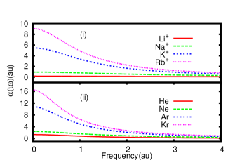
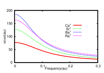
Comparison between these results show that our methods are giving reasonably accurate $\alpha(0)$ values, thus these methods can be employed to determine dynamic polarizabilities in these atomic systems within the similar accuracies as observed in the evaluation of the scalar polarizabilities. We plot these dynamic polarizabilities in Figs. 1 and 2. As seen from the figures, alkaline earth ions have the highest polarizabilities, followed by inert gas atoms and then alkali ions.

Using the dynamic polarizabilities given above, we now determine the dispersion coefficients of the considered alkali ions, alkaline-earth ions, and inert gas atoms interacting with a graphene layer with the reflection coefficients estimated using the Dirac model. This is an extension of our previous work  Kaur et al. (2014), where the interaction of the alkali atoms with a graphene layer is investigated. Here, we adopt the approaches described in Refs.  Arora et al. (2014); Chaichian et al. (2012) to evaluate the reflection coefficients for the determination of $C_{3}$ coefficients as a function of separation distance of an atomic system from the graphene layer and a function of temperature. These results are discussed systematically below for each class of atomic systems.

Figure 3: (Color online) The $C_{3}$ coefficients (in au) as function of the ion-graphene separation distance for the alkali metal ions Li⁺, Na⁺, K⁺ and Rb⁺ interacting at $T=300^{\circ}$ K (solid red curve) and $T=0^{\circ}$ K (dashed green curve).

IV.1 Interactions of alkali ions with a graphene layer

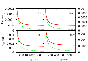
In Fig. 3, the graph between $C_{3}$ coefficients as a function of the separation distance $a$ (in nm) for the interactions of alkali ions Li⁺, Na⁺, K⁺ and Rb⁺ with a graphene layer is shown for a gap parameter $\Delta=0.01$ eV. The solid red curve corresponds to the room temperature $T=300$ K while the dashed green curve represents $T=0$ K temperature $C_{3}$ coefficients. It should be noted that the reflection coefficients being same for a particular interacting surface (in our case, graphene), at a specific separation distance and temperature, the $C_{3}$ coefficients of an element completely depends on its dynamic dipole polarizabilities. It was found in  Arora et al. (2014) that the $C_{3}$ coefficients increases with corresponding increase in atomic sizes of the alkali atoms for a given separation distance. In the same manner, it is seen that there is a likewise increase in the dispersion $C_{3}$ coefficients with the increase in the size of alkali ions at a particular distance of separation. It can also be observed from this figure that the interaction between these ions and a graphene layer are more effective at the short separations while they are negligible at large separation distances.

Figure 4: (Color online) The $C_{3}$ coefficients (in au) calculated for the interactions of the alkaline-earth ions Ca⁺, Sr⁺, Ba⁺ and Ra⁺ with a graphene layer as function of separation distance ‘$a$’ (in nm) at temperatures $T=300^{\circ}$ K (red solid curve) and $T=0^{\circ}$ K (green dashed curve).

Figure 5: (Color online) The $C_{3}$ coefficients (in au) for the interactions of the inert gas atoms He, Ne, Ar and Kr with graphene as function of the separation distance ‘$a$’ (in nm) at temperatures $T=300^{\circ}$ K (shown solid red curve) and $T=0^{\circ}$ K (shown dashed green curve).

IV.2 Interactions of alkaline-earth ions with graphene

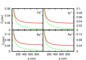
The dispersion interactions of the alkaline-earth ions Ca⁺, Sr⁺, Ba⁺ and Ra⁺ with a graphene layer at temperatures $T=300$ K (solid red curve) and $T=0$ K (dashed green curve) are shown in Fig. 4. It can be clearly seen from this figure that these $C_{3}$ coefficients are large for comparatively large ions except for the Ba⁺ ion. This dominance of Ba⁺ ion $C_{3}$ coefficient over the Ra⁺ ion coefficient is due to the fact that the polarizabilty of Ba⁺ ion is larger than that of Ra⁺  Sahoo and Das (2008); Safronova et al. (2007); Kaur et al. (2015). The reduction in the polarizability of Ra⁺ ion is owing to the domineering contribution of the relativistic effects over the correlation effects  Lim and Schwerdtfeger (2004). Again, it can be seen in the figure that the interaction between these ions with a graphene layer are more effective at the short separations and becomes insignificant at the large separation distances. Among the three types of atomic systems, interaction of graphene with alkaline-earth ions is the strongest one. For a separation distance of 300 nm, the interaction of alkaline earth ions with graphene layer is approximately 14 times stronger than the interaction with alkali ions, whereas approximately 8 times stronger than the interaction with inert gas atoms.

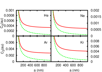
IV.3 Interactions of inert gas atoms with graphene

The graph for the interactions between the inert gas atoms with a graphene layer, as a function of separation distance ‘$a$’, is presented in Fig. 5. We can clearly observe from the figure that $C_{3}$ coefficients of the ion-graphene interactions are large for comparatively large ions, owing to their greater values of scalar polarizabilities. These coefficients are shown for temperatures $T=300$ K (solid red curve) and $T=0$ K (dashed green curve). It can be seen from Fig. 5 that the dispersion coefficients calculated at the room temperature show very less variation from the zero temperature coefficients at small separations whereas, at the larger distances of separations, we find a comparatively stronger dispersion interactions at $T=300$ K as compared to interaction at $T=0$ K.

Table 2: Fitting parameters for the $C_{3}$(a, $T=300$ K) coefficients of the considered alkali ions, alkaline-earth ions and inert gas atoms with a graphene layer. A₁ and A₂ are given in the order of 10^-2 au and $x_{0}$ in nm.

Alkali ions	Li+	Na+	K+	Rb+
A1	0.48798	2.41443	13.3224	21.6418
A2	0.00368	0.01841	0.10702	0.17863
$x_{0}$	1.5239	1.53425	1.58631	1.61405
Alkaline earth ions	Ca+	Sr+	Ba+	Ra+
A1	66.8551	100.604	136.182	137.158
A2	1.71017	2.84881	4.19032	3.66618
$x_{0}$	3.28993	3.49327	3.64421	3.31959
Inert gas atoms	He	Ne	Ar	Kr
A1	3.214	5.8524	24.7463	36.6345
A2	0.02594	0.04662	0.2133	0.32761
$x_{0}$	1.59107	1.57743	1.65885	1.69824

IV.4 Fitting Formula

In contemplation of simplification in generating our results of $C_{3}$ coefficients for future theoretical and experimental verifications or for extracting these values for various applications at room temperature with a given separation distance, we provide a logistic fit of the functional form of these coefficients as

$$C_{3}(a)=A_{2}+\frac{A_{1}-A_{2}}{(1+{a/x_{0}})},$$ (11)

where $A_{1}$ (in au), $A_{2}$ (in au) and $x_{0}$ (in nm) are the fitting parameters that rely on the properties of the interacting atomic systems with a graphene layer. We give our fitting coefficients in Table  2 for extrapolating the dispersion coefficients for the considered elements-graphene layer interactions. We predict that obtained coefficients using above fitting parameters have divergences not more than 6 % with the coefficients calculated using Dirac model at $T=300$ K. Hence, the above equation serves as the best suited fit to express the interactions of considered atomic systems with a graphene layer.

V Conclusion

In summary, we have studied the dispersion interaction coefficients of the alkali-metal ions (Li⁺, Na⁺, K⁺ and Rb⁺), alkaline-earth ions (Ca⁺, Sr⁺, Ba⁺ and Ra⁺) and inert gas atoms (He, Ne, Ar and Kr) with a graphene layer. We have shown explicitly the dependence of these coefficients on the separation distance $a$ and temperature $T$. We have commenced by using accurate values of the dynamic polarizabilities of the considered atomic systems by employing suitable relativistic many-body methods and calculating the reflection coefficients using the Dirac model. We observed that the dispersion interaction coefficients of the alkaline ions with the graphene layer is the strongest among the alkali ions and inert gas atoms interacting with graphene; the least dispersion interaction of graphene is with the alkali ions. It is also seen that due to the larger values of dynamic polarizabilities of the Ba⁺ ion than that of Ra⁺ ion, the dispersion coefficient of Ba⁺ dominates over the Ra⁺ ion. Our results can be of utmost use for the experimentalists in studying these interactions more reliably in view of the fact that performing these experiments at room temperature are comparatively more susceptible. This study also demonstrates about stronger dispersion interactions of the alkaline ions, especially at the larger distances of separations, and its consequences can be more applicably. In addition, we also devise a promptly accessible functional form of logistic type having separation distance dependence at room temperature for easy extraction of the dispersion coefficients for the future applications.

References

- Novoselov et al. (2004) K. S. Novoselov, A. K. Geim, S. V. Morozov, D. Jiang, Y. Zhang, S. V. Dubonos, I. V. Grigorieva, and A. A. Firsov, Science 306, 666 (2004).
- Geim and Novoselov (2007) A. K. Geim and K. S. Novoselov, Nature Materials 6, 183 (2007).
- Friedrich et al. (2002) H. Friedrich, G. Jacoby, and C. G. Meister, Phys. Rev. A 65, 032902 (2002).
- Iijima (1991) S. Iijima, Nature 354, 56 (1991).
- Ebbesen and Ajayan (1992) T. W. Ebbesen and P. M. Ajayan, Nature 358, 220 (1992).
- Guo et al. (1995) T. Guo, P. Nikolaev, A. G. Rinzler, D. Tomanek, D. T. Colbert, and R. E. Smalley, J. Phys. Chem. 99, 1069410697 (1995).
- Mowbray et al. (2006) D. J. Mowbray, Z. L. Miskovic, and F. O. Goodman, Phys. Rev. B 74, 195435 (2006).
- Novoselov et al. (2012) K. S. Novoselov, V. I. Fal’ko, L. Colombo, P. R. Gellert, M. G. Schwab, and K. Kim, Nature 490, 192 (2012).
- Zhang et al. (2011) Q. Zhang, S. Wu, L. Zhang, J. Lu, F. Verproot, Y. Liu, Z. Xing, J. Li, and X. M. Song, Biosens. Bioelectron 26, 2632 (2011).
- Chan and Hill (2010) Y. Chan and J. M. Hill, Micro Nano Lett. 5, 247 (2010).
- Hilder and Hill (2007) T. A. Hilder and J. M. Hill, Curr. Appl. Phys. 8, 258 (2007).
- Tang and Cao (2011) S. Tang and Z. Cao, J. Chem. Phys. 134, 044710 (2011).
- Wang et al. (2010) Y. Wang, Y. Shao, D. W. Matsun, J. Li, and Y. Lin, ACS Nano 4, 1790 (2010).
- Kaur et al. (2014) K. Kaur, J. Kaur, B. Arora, and B. K. Sahoo, Phys. Rev. B 90, 245405 (2014).
- Arora et al. (2014) B. Arora, H. Kaur, and B. K. Sahoo, J. Phys. B: At. Mol. Opt. Phys. 47, 155002 (2014).
- Dino et al. (2004) W. A. Dino, H. Nakanishi, and H. Kasai, e-J. Surf. Sci. Nanotechnol. 2, 77 (2004).
- Bogicevic et al. (2000) A. Bogicevic, S. Ovesson, P. Hyldgaard, B. I. Lundqvist, H. Brune, and D. R. Jennison, Phys. Rev. Lett. 85, 1910 (2000).
- Jung et al. (2004) J. Jung, P. Garcia-Gonzalez, J. F. Dobson, and R. W. Godby, Phys. Rev. B 70, 205107 (2004).
- Dobson et al. (2006) J. F. Dobson, A. White, and A. Rubio, Phys. Rev. Lett. 96, 073201 (2006).
- Hult et al. (2001) E. Hult, P. Hyldgaard, J. Rossmeisl, and B. I. Lundqvist, Phys. Rev. B 64, 195414 (2001).
- Bondarev and Lambin (2004) I. V. Bondarev and P. Lambin, Phys. Rev. B 70, 035407 (2004).
- Churkin et al. (2010) Y. V. Churkin, A. B. Fedortsov, G. L. Klimchitskaya, and V. A. Yurova, Phys. Rev. B 82, 165433 (2010).
- Caride et al. (2005) A. O. Caride, G. L. Klimchitskaya, V. M. Mostepanenko, and S. I. Zanette, Phys. Rev. A 71, 042901 (2005).
- Blagov et al. (2005) E. V. Blagov, G. L. Klimchitskaya, and V. M. Mostepanenko, Phys. Rev. B 71, 235401 (2005).
- Babb et al. (2004) J. F. Babb, G. L. Klimchitskaya, and V. M. Mostepanenko, Phys. Rev. A 70, 042901 (2004).
- Chaichian et al. (2012) M. Chaichian, G. L. Klimchitskaya, V. M. Mostepanenko, and A. Tureanu, Phys. Rev. A 86, 012515 (2012).
- Bordag (2006) M. Bordag, J. Phys. A: Math. Gen. 39, 6173 (2006).
- Jiang and M. H. Du (2009) D. Jiang and S. D. M. H. Du, J. Chem. Phys. 130, 074705 (2009).
- Wintterlin and Bocquet (2009) J. Wintterlin and M. L. Bocquet, Surf. Sci. 603, 1841 (2009).
- Dresselhaus and Dresselhaus (2002) M. S. Dresselhaus and G. Dresselhaus, Adv. Phys. 51, 1 (2002).
- Yang (2009) C. K. Yang, Appl. Phys. Lett. 94, 163115 (2009).
- kai Konga and wang Chen (2013) X. kai Konga and Q. wang Chen, Phys. Chem. Chem. Phys. 15, 12982 (2013).
- Burress et al. (2010) J. W. Burress, S. Gadipelli, J. Ford, J. M. Simmons, W. Zhou, and T. Yildirim, Angew. Chem. Int. 49, 8902 (2010).
- Tozzini and Pellegrini (2013) V. Tozzini and V. Pellegrini, Phys. Chem. Chem. Phys. 15, 80 (2013).
- Spyrou et al. (2013) K. Spyrou, D. Gournis, and P. Rudolf, ECS J. Solid State Sci. Technol. 2, M3160 (2013).
- Bordag et al. (2001) M. Bordag, U. Mohideen, and V. M. Mostepanenko, Phys. Rep. 353, 1 (2001).
- andB. Geyer et al. (2006) M. B. andB. Geyer, G. L. Klimchitskaya, and V. M. Mostepanenko, Phys. Rev. B 74, 205431 (2006).
- Blagov et al. (2007) E. V. Blagov, G. L. Klimchitskaya, and V. M. Mostepanenko, Phys. Rev. B 75, 235413 (2007).
- Bordag et al. (2009a) M. Bordag, I. V. Fialkovsky, D. M. Gitman, and D. V. Vassilevich, Phys. Rev. B 80, 245406 (2009a).
- Churkin et al. (2011) Y. V. Churkin, A. B. Fedortsov, G. L. Klimchitskaya, and V. A. Yurova, International Journal of Modern Physics:Conference Series 3, 555 (2011).
- Bordag et al. (2009b) M. Bordag, G. Klimchitskaya, U. Mohideen, and V. Mostepanenko, Advances in the Casimir Effect (Oxford University Press, Oxford, 2009b).
- Semenoff (1984) G. W. Semenoff, Phys. Rev. Lett. 53, 2449 (1984).
- DiVincenzo and Mele (1984) D. P. DiVincenzo and E. J. Mele, Phys. Rev. B 29, 1685 (1984).
- Drosdoff and Woods (2010) D. Drosdoff and L. M. Woods, Phys. Rev. B 82, 155459 (2010).
- Sernelius (2011) B. E. Sernelius, Europhys. Lett. 95, 57003 (2011).
- Sarabadani et al. (2011) J. Sarabadani, A. Naji, R. Asgari, and R. Podgornik, Phys. Rev. B 84, 155407 (2011).
- Drosdoff et al. (2012) D. Drosdoff, A. D. Phan, L. M. Woods, I. V. Bondarev, and J. F. Dobson, Eur. Phys. J. B 85, 365 (2012).
- Fialkovsky et al. (2011) I. V. Fialkovsky, V. N. Marachevsky, and D. V. Vassilevich, Phys. Rev. B 84, 035446 (2011).
- Kaur et al. (2015) J. Kaur, D. K. Nandy, B. Arora, and B. K. Sahoo, Phys. Rev. A 91, 012705 (2015).
- Johnson et al. (1983) W. R. Johnson, D. Kolb, and K. Huang, At. Data Nucl. Data Tables 28, 333 (1983).
- Bhatia and Drachman (1997) A. K. Bhatia and R. J. Drachman, Can. J. phys. 75, 11 (1997).
- Cooke et al. (1977) W. E. Cooke, T. F. Gallagher, R. M. Hill, and S. A. Edelstein, Phys. Rev. A 16, 1141 (1977).
- Singh et al. (2013) Y. Singh, B. K. Sahoo, and B. P. Das, Phys. Rev. A 88, 062504 (2013).
- Lim et al. (2002) I. S. Lim, J. K. Laerdahl, and P. Schwerdtfeger, J. Chem. Phys. 116, 172 (2002).
- Opik (1967) U. Opik, Phys. Soc. 92, 566 (1967).
- Johansson (1961) I. Johansson, Ark. Fys. 20, 135 (1961).
- Lim and Schwerdtfeger (2004) I. S. Lim and P. Schwerdtfeger, Phys. Rev. A 70, 062501 (2004).
- Mitroy and Zhang (2008) J. Mitroy and J. Y. Zhang, Eur. Phys. J. D. 46, 415 (2008).
- Chang (1983) E. S. Chang, J. Phys. B 16, L539 (1983).
- Sahoo et al. (2009a) B. K. Sahoo, B. P. Das, and D. Mukherjee, Phys. Rev. A 79, 052511 (2009a).
- Arora et al. (2007) B. Arora, M. S. Safronova, and C. Clark, Phys. Rev. A 76, 064501 (2007).
- Patil and Tang (1997) S. H. Patil and K. T. Tang, J. Chem. Phys. 106, 2298 (1997).
- Sahoo et al. (2009b) B. K. Sahoo, R. G. E. Timmermans, B. P. Das, and D. Mukherjee, Phys. Rev. A 80, 062506 (2009b).
- Barklem and O’Mara (2000) P. S. Barklem and B. J. O’Mara, Mon. Not. R. Astron. Soc. 311, 535 (2000).
- Jiang et al. (2009) D. Jiang, B. Arora, M. S. Safronova, and C. W. Clark, J. Phys. B 42, 154020 (2009).
- Snow and Lundeen (2007) E. L. Snow and S. R. Lundeen, Phys. Rev. A 76, 052505 (2007).
- Safronova et al. (2007) U. I. Safronova, W. R. Johnson, and M. S. Safronova, Phys. Rev. A 76, 042504 (2007).
- Sahoo et al. (2007) B. K. Sahoo, B. P. Das, R. K. Chaudhuri, D. Mukherjee, R. G. E. Timmermans, and K. Jungmann, Phys. Rev. A 76, 040504(R) (2007).
- Pal et al. (2009) R. Pal, D. Jiang, M. S. Safronova, and U. I. Safronova, Phys. Rev. A 79, 062505 (2009).
- Soldan et al. (2001) P. Soldan, E. P. F. Lee, and T. G. Wright, Phys. Chem. 3, 4661 (2001).
- Langhoff and Karplus (1969) P. W. Langhoff and M. Karplus, J. Opt. Soc. Am. 59, 863 (1969).
- Nakajima and Hirao (2001) T. Nakajima and K. Hirao, Chem. Lett. 30, 766 (2001).
- Singh et al. (2014) Y. Singh, B. K. Sahoo, and B. P. Das, Phys. Rev. A 89, 030502(R) (2014), erratum, Phys. Rev. A 90, 039903(E) (2014).
- Sahoo and Das (2008) B. K. Sahoo and B. P. Das, Phys. Rev. A 77, 062516 (2008).