Finite-temperature quantum criticality in a complex-parameter plane

Abstract

A conventional quantum phase transition (QPT) occurs not only at zero temperature, but also exhibits finite-temperature quantum criticality. Motivated by the discovery of the pseudo-Hermiticity of non-Hermitian systems, we explore the finite-temperature quantum criticality in a non-Hermitian $\mathcal{PT}$-symmetric Ising model. We present the complete set of exact eigenstates of the non-Hermitian Hamiltonian, based on which the mixed-state fidelity in the context of biorthogonal bases is calculated. Analytical and numerical results show that the fidelity approach to finite-temperature QPT can be extended to the non-Hermitian Ising model. This paves the way for experimental detection of quantum criticality in a complex-parameter plane.

I Introduction

A central task of the theory of quantum phase transitions (QPTs) is to describe the consequences of this zero temperature singularity on physical properties at finite temperature since all experiments can only be done at non-zero temperature S.Sachdev . It turns out that the mixed-state fidelity, which is related to the statistical distance between two density operators, is a powerful way to describe the signatures of QPTs at nonzero temperature Sun .

Recently, there have been intense efforts to establish a $\mathcal{PT}$-symmetric quantum theory as a complex extension of the conventional quantum mechanics Bender 98 ; Bender 99 ; Dorey 01 ; Bender 02 ; A.M43 ; A.M ; A.M36 ; Jones ; AM , since the discovery that a non-Hermitian Hamiltonian having simultaneous parity-time ($\mathcal{PT}$) symmetry has a real spectrum Bender 98 . Motivated by the pseudo-Hermiticity of non-hermitian systems, the QPT in a non-Hermitian $\mathcal{PT}$-symmetric Ising model, which is driven by a complex staggered transverse field, has been explored based on the exact solution Li . It has been shown that the phase diagram can be characterized by the geometric phase. The phase boundary can be identified by a divergence of Berry curvature density, which is defined in the context of biorthogonal bases.

In this paper, we address two questions concerning the quantum criticality for the non-hermitian Ising model at finite temperature. At first, whether the QPT driven by complex parameters has residual criticality at finite temperature. Second, as a metric-based approach, whether the mixed-state fidelity in the context of biorthogonal bases is available to describe this criticality. Analytical and numerical results indicate that the phase boundary at finite temperature can be identified by the mixed-state fidelity.

The paper is organized as follows: In Sec. II we present the exact solution of the non-Hermitian Ising model. In Sec. III, the mixed-state fidelity of thermal states is obtained analytically and a numerical simulation is performed to demonstrate the signatures of QPTs at finite temperature. Section IV contains the conclusion.

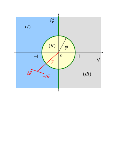
Figure 1: (Color online) Phase diagram for the ground state of the Ising ring in a complex staggered transverse field. The heavy lines (green) represent the boundary which separates three quantum phases. Phases I and III are paramagnet, while II is ferromagnet. Vector $\overrightarrow{r}$ denotes an arbitrary position in the $\xi\eta$ plane, while $\overrightarrow{r}\pm\Delta\overrightarrow{r}$ are two points in the vicinity of point $\overrightarrow{r}$. The mixed-state fidelity for those two points can characterize the thermal criticality at point $\overrightarrow{r}$.

II Model and solution

In the last few years, there have been many studies of the phase diagrams for various quantum models in the aid of the fidelity Zanardi ; Vezzani ; Chen ; Yang ; Huan ; Alet ; Rams or mixed-state fidelity Sun ; Vieira ; Quan ; Sirker . All the investigations are performed for Hermitian Hamiltonians, where the probability is preserving in the context of standard Dirac inner product. It would be interesting to explore the extension of this metric-based approach to a non-Hermitian Hamiltonian with pseudo-Hermiticity, where biorthonormal inner product is introduced. We begin our investigation by introducing a non-Hermitian Ising model, whose ground state phase diagram has been studied in previous work Li . It has been shown that the Berry phase in the context of biorthonormal inner product can identify the phase diagram, which sheds some light on the extension of the metric-based approach to a non-Hermitian system.

The concept is studied exemplarily for criticality in a non-Hermitian one-dimensional spin-$1/2$ Ising model with a complex staggered transverse magnetic field on a $2N$-site lattice. The system is modeled by the following Hamiltonian

$$\mathcal{H}\text{ }=-J\underset{j=1}{\overset{2N}{\sum}}\left(\sigma_{j}^{z}\sigma_{j+1}^{z}+g_{{}_{j}}\sigma_{j}^{x}\right),$$ (1)

where complex field $g_{{}_{j}}=\eta+i\left(-1\right)^{j}\xi$ ($i=\sqrt{-1}$) with $\eta$ and $\xi$ being real numbers. Here $\sigma_{j}^{\lambda}$ ($\lambda=x,$ $z$) are the Pauli operators on site $j$, and satisfy the periodic boundary condition $\sigma_{j}^{\lambda}\equiv\sigma_{j+2N}^{\lambda}$. In ground state this model exhibits quantum critical points at $\eta^{2}+\xi^{2}=1$ and $\eta=0$ for $\eta^{2}+\xi^{2}>1$, separating paramagnetic and ferromagnetic phases Li .

Following the derivation in Appendix, all the eigenstates of $\mathcal{H}$ can be constructed as the form

$$\left|\Psi\right\rangle=\prod_{k\in\left[0,\pi\right]}\overline{\left|n\right\rangle}_{k},$$ (2)

with eigen energy

$$E=\sum_{\left\{\overline{\left|n\right\rangle}_{k}\right\}}\epsilon^{n}\left(k\right).$$ (3)

Here $\overline{\left|n\right\rangle}_{k}$ $\left(n\in\left[1,16\right]\right)$ denotes the $16$-dimensional qudit ($16$-level system) state, which is expressed explicitly as

$$n\in\left[1,5\right]:\overline{\left|n\right\rangle}_{k}$$ (4)

$$= \frac{1}{\Omega^{n}}[2\cos\left(k/2\right)\left(\frac{\alpha_{k}^{\dagger}\alpha_{-k}^{\dagger}}{\epsilon^{n}+i2\xi}+\frac{\beta_{k}^{\dagger}\beta_{-k}^{\dagger}}{\epsilon^{n}-i2\xi}\right)$$

$$-2i\sin\left(k/2\right)\left(\frac{1}{\epsilon^{n}+2\eta}\alpha_{k}^{\dagger}\beta_{k}^{\dagger}\alpha_{-k}^{\dagger}\beta_{-k}^{\dagger}+\frac{1}{\epsilon^{n}-2\eta}\right)$$

$$+e^{ik/2}\alpha_{k}^{\dagger}\beta_{-k}^{\dagger}-e^{-ik/2}\beta_{k}^{\dagger}\alpha_{-k}^{\dagger}]\left|0\right\rangle,$$

and

$$\overline{\left|6\right\rangle}_{k} = \frac{1}{\sqrt{2}}\left(e^{ik/2}\alpha_{k}^{\dagger}\beta_{-k}^{\dagger}+e^{-ik/2}\beta_{k}^{\dagger}\alpha_{-k}^{\dagger}\right)\left|0\right\rangle,$$

$$\overline{\left|\overline{7}\right\rangle}_{k} = \alpha_{k}^{\dagger}\beta_{k}^{\dagger}\left|0\right\rangle\text{, }\left|\overline{8}_{k}\right\rangle=\alpha_{-k}^{\dagger}\beta_{-k}^{\dagger}\left|0\right\rangle,$$ (5)

and

$$n \in \left[9,12\right]:\overline{\left|n\right\rangle}_{k}$$ (6)

$$= \frac{1}{\Omega^{n}}\{\{\left(\epsilon^{n}+\eta-i\xi\right)[\left(\epsilon^{n}\right)^{2}-\left(\eta+i\xi\right)^{2}-1]$$

$$-2(\eta\cos^{2}\frac{k}{2}-i\xi\sin^{2}\frac{k}{2})\}e^{-ik/2}\alpha_{k}^{\dagger}$$

$$+[\left(\epsilon^{n}+\eta\right)^{2}+\xi^{2}-1]\cos\frac{k}{2}\beta_{k}^{\dagger}$$

$$-i[\left(\epsilon^{n}-i\xi\right)^{2}-\eta^{2}-1]\sin\frac{k}{2}\alpha_{-k}^{\dagger}\alpha_{k}^{\dagger}\beta_{k}^{\dagger}$$

$$-i\left(\eta+i\xi\right)\sin ke^{-ik/2}\alpha_{k}^{\dagger}\beta_{-k}^{\dagger}\beta_{k}^{\dagger}\}\left|0\right\rangle,$$

and

$$n \in \left[12,16\right]:\overline{\left|n\right\rangle}_{k}$$ (7)

$$= \frac{1}{\Omega^{n}}\{\{\left(\epsilon^{n}+\eta-i\xi\right)[\left(\epsilon^{n}\right)^{2}-\left(\eta+i\xi\right)^{2}-1]$$

$$-2(\eta\cos^{2}\frac{k}{2}-i\xi\sin^{2}\frac{k}{2})\}e^{-ik/2}\alpha_{-k}^{\dagger}$$

$$+[\left(\epsilon^{n}+\eta\right)^{2}+\xi^{2}-1]\cos\frac{k}{2}\beta_{-k}^{\dagger}$$

$$-i[\left(\epsilon^{n}-i\xi\right)^{2}-\eta^{2}-1]\sin\frac{k}{2}\alpha_{k}^{\dagger}\alpha_{-k}^{\dagger}\beta_{-k}^{\dagger}$$

$$-i\left(\eta+i\xi\right)\sin ke^{-ik/2}\alpha_{-k}^{\dagger}\beta_{k}^{\dagger}\beta_{-k}^{\dagger}\}\left|0\right\rangle,$$

where $\Omega^{n}$ is corresponding normalization factor. And coefficients $\epsilon^{n}\left(k\right)$ are given as

$$\epsilon^{1} = [2r^{2}\cos\left(2\varphi\right)+2+2\sqrt{r^{4}-2r^{2}\cos k+1}]^{1/2},$$

$$\epsilon^{3} = [2r^{2}\cos\left(2\varphi\right)+2-2\sqrt{r^{4}-2r^{2}\cos k+1}]^{1/2},$$

$$\epsilon^{2} = -\epsilon^{1},\epsilon^{4}=-\epsilon^{3},\text{ }\epsilon^{5}=\epsilon^{6}=\epsilon^{7}=\epsilon^{8}=0,$$

$$\epsilon^{9} = [r^{2}\cos\left(2\varphi\right)+1$$

$$+\sqrt{4r^{2}\cos^{2}\varphi+2r^{2}\cos k-2r^{4}}]^{1/2},$$

$$\epsilon^{11} = [r^{2}\cos\left(2\varphi\right)+1$$

$$-\sqrt{4r^{2}\cos^{2}\varphi+2r^{2}\cos k-2r^{4}}]^{1/2},$$

$$\epsilon^{14} = -\epsilon^{13}=\epsilon^{10}=-\epsilon^{9},\text{ }$$

$$\epsilon^{16} = -\epsilon^{15}=\epsilon^{12}=-\epsilon^{11}.$$ (8)

Here $\alpha_{k}^{\dagger}$ and $\beta_{k}^{\dagger}$ are fermionic creation operators and we parameterize the complex field in terms of the polar radius and angle

$$r=\sqrt{\eta^{2}+\xi^{2}}\text{ and }\tan\varphi=\xi/\eta.$$ (9)

Similarly, we can obtain the eigenstates of $\mathcal{H}^{{\dagger}}$ by the qudit state $\left\langle n\right|_{k}$, which has the form

$$\left\langle n\left(\xi\right)\right|_{k}=\left(\overline{\left|n\left(-\xi\right)\right\rangle}_{k}\right)^{{\dagger}}.$$ (10)

It is turned out that the complete biorthonormal set can be constructed due to the fact

$$\left\langle n\right|_{k}\overline{\left|m\right\rangle}_{k^{\prime}}=\delta_{mn}\delta_{kk^{\prime}}\text{, }\sum_{n}\overline{\left|n\right\rangle}_{k}\left\langle n\right|_{k}=1.$$ (11)

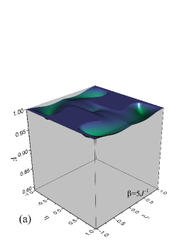
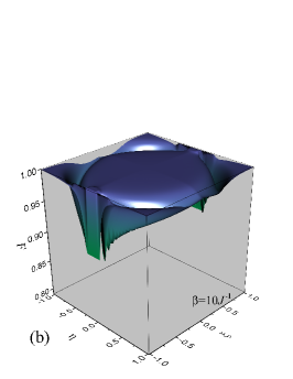
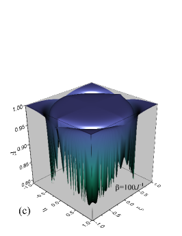
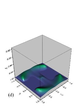
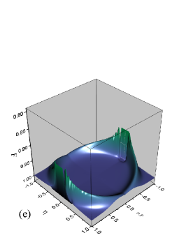
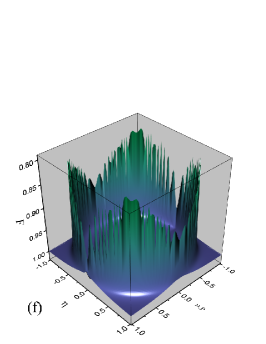
Figure 2: (Color online) $3$-D plots of mixed-state fidelity of finite-temperature thermal state of the non-Hermitian Ising model. We consider the case with $N=300$ and the field variances $\Delta\eta=\Delta\xi=0.01J^{-1}$. Figures (a-c) plots of $F$ as functions of $\eta$ and $\xi$ for different temperatures $\beta$, while (d-f) are corresponding inversions of (a-c). At high temperatures (a), the mixed-state fidelity shows a flat surface. When the temperature decreases (b, c), the decay of fidelity becomes sharp and clearly shows the signature of QPT which occurs at absolute zero temperature. A more accurate dependence is plotted in Fig.3.

At zero-temperature, the phase diagram is obtained in Ref. Li and sketched in Fig.1. The influence of the imaginary field $i\xi$ on the phase transition is obvious: It enhances the action of the real transverse field $\eta$, shrinking the disorder region, leading to a circular phase boundary. In the following, we will show that this circle critical line is still robust at finite temperature.

III Mixed-state fidelity

The key point of this paper is that the mixed-state fidelity

$$F\left(\rho,\widetilde{\rho}\right)=\mathrm{tr}\sqrt{\widetilde{\rho}^{1/2}\rho\widetilde{\rho}^{1/2}}$$ (12)

can be utilized to characterize the thermal criticality although density matrices $\rho$ and $\widetilde{\rho}$ are non-Hermitian. The non-Hermiticity of the matrices arises from the description of two different thermal states

$$\rho = \exp\left(-\beta\mathcal{H}\right)/\mathrm{tr}\exp\left(-\beta\mathcal{H}\right),$$ (13)

$$\widetilde{\rho} = \exp\left(-\beta\widetilde{\mathcal{H}}\right)/\mathrm{tr}\exp\left(-\beta\widetilde{\mathcal{H}}\right),$$ (14)

where

$$\mathcal{H}=\mathcal{H}\left(\eta,\xi\right),\widetilde{\mathcal{H}}=\mathcal{H}\left(\eta+\delta\eta,\xi+\delta\eta\right),$$ (15)

are both non-Hermitian operators.

As the consequence of the translational symmetry, $\left[h_{k},h_{k^{{}^{\prime}}}\right]=0$, leads to

$$F\left(\rho,\widetilde{\rho}\right)=\prod_{k}\mathrm{tr}\sqrt{\rho_{k}^{1/2}\widetilde{\rho}_{k}\rho_{k}^{1/2}},$$ (16)

which can simplify the computation procedure. Studies on Hermitian systems show that a zero-temperature fidelity vanishes at the quantum boundary. It is expected that the similar behavior can occur for the present non-Hermitian model. Actually, in the limit case $\beta\rightarrow\infty$, $F\left(\rho,\widetilde{\rho}\right)$ is reduced to

$$F_{\infty}\left(\rho,\widetilde{\rho}\right)=\prod_{k}O_{k}=\prod_{k}\left|\widetilde{\left\langle 1\right|}_{k}\overline{\left|1\right\rangle}_{k}\right|,$$ (17)

by using the completeness condition in Eq. (11). Here states $\widetilde{\left\langle 1\right|}_{k}$ and $\overline{\left|1\right\rangle}_{k}$ are

$$\widetilde{\left\langle 1\right|}_{k}=\left\langle 1\left(\overrightarrow{r}+\Delta\overrightarrow{r}\right)\right|_{k},\overline{\left|1\right\rangle}_{k}=\overline{\left|1\left(\overrightarrow{r}-\Delta\overrightarrow{r}\right)\right\rangle}_{k},$$ (18)

where $\overrightarrow{r}$ denotes a vector in the $\xi\eta$ plane (see Fig.1). In the following, we consider a simple case with $\overrightarrow{r}=$ $\left(\cos\varphi,\sin\varphi\right)$ and $\Delta\overrightarrow{r}=$ $\left(\Delta r\cos\varphi,\Delta r\sin\varphi\right)$. Correspondingly, states $\widetilde{\left\langle 1\right|}_{k}$ and $\overline{\left|1\right\rangle}_{k}$ can be expressed in a polar coordinate system $(r,\varphi)$

$$\widetilde{\left\langle 1\right|}_{k}=\left\langle 1\left(1+\Delta r,\varphi\right)\right|_{k},\overline{\left|1\right\rangle}_{k}=\overline{\left|1\left(1-\Delta r,\varphi\right)\right\rangle}_{k}.$$ (19)

We note that any vanishing overlaps $\widetilde{\left\langle 1\right|}_{k}\overline{\left|1\right\rangle}_{k}$ can result in the zero point of fidelity $F_{\infty}\left(\rho,\widetilde{\rho}\right)$. In the thermodynamic limit $N\rightarrow\infty$, $k$ becomes a continuous variable. This ensures us to estimate the overlap $\lim_{k\rightarrow 0}\widetilde{\left\langle 1\right|}_{k}\overline{\left|1\right\rangle}_{k}$. Direct derivation shows that

$$\lim_{k\rightarrow 0}\overline{\left|1\left(r,\varphi\right)\right\rangle}_{k}=\frac{1}{\gamma+\gamma^{\ast}}(\alpha_{k}^{\dagger}\beta_{-k}^{\dagger}-\beta_{k}^{\dagger}\alpha_{-k}^{\dagger}$$

$$+\gamma^{\ast}\alpha_{k}^{\dagger}\alpha_{-k}^{\dagger}+\gamma\beta_{k}^{\dagger}\beta_{-k}^{\dagger})\left|0\right\rangle\text{, }\left(r<1\right),$$ (20)

and

$$\lim_{k\rightarrow 0}\widetilde{\left\langle 1\left(r,\varphi\right)\right|}_{k}=\left\langle 0\right|i\text{, }\left(r>1\right),$$ (21)

where $\varphi\in\left[0,\frac{\pi}{2}\right)\cup\left(\frac{3\pi}{2},2\pi\right]$, and $\gamma=\sqrt{1-r^{2}\sin\varphi}+ir\sin\varphi$. Meanwhile we have

$$\lim_{k\rightarrow 0}\overline{\left|1\left(r,\varphi\right)\right\rangle}_{k}=\frac{1}{\gamma+\gamma^{\ast}}(\alpha_{k}^{\dagger}\beta_{-k}^{\dagger}-\beta_{k}^{\dagger}\alpha_{-k}^{\dagger}$$

$$+\gamma^{\ast}\alpha_{k}^{\dagger}\alpha_{-k}^{\dagger}+\gamma\beta_{k}^{\dagger}\beta_{-k}^{\dagger})\left|0\right\rangle\text{, }\left(r<1\right),$$ (22)

and

$$\lim_{k\rightarrow 0}\widetilde{\left\langle 1\left(r,\varphi\right)\right|}_{k}=\left\langle 0\right|i\alpha_{k}\beta_{k}\alpha_{-k}\beta_{-k}\text{, }\left(r>1\right),$$ (23)

where $\varphi\in\left(\frac{\pi}{2},\frac{3\pi}{2}\right)$. These lead to the conclusion that

$$\lim_{k\rightarrow 0}\left\langle 1\left(1+\Delta r,\varphi\right)\right|_{k}\overline{\left|1\left(1-\Delta r,\varphi\right)\right\rangle}_{k}=0,$$ (24)

for $\Delta r>0$ and $\varphi\neq\frac{\pi}{2},\frac{3\pi}{2}$. The essence of the results is the nonanalytical behavior of states $\lim_{k\rightarrow 0}\widetilde{\left\langle 1\right|}_{k}$ and $\lim_{k\rightarrow 0}\overline{\left|1\right\rangle}_{k}$ at the critical points. This indicates that the fidelity approach for QPT can be extended into the complex regime at zero temperature.

However, the overlap in both points $\varphi_{0}=\frac{\pi}{2}$ and $\frac{3\pi}{2}$ can be calculated analytically as

$$\lim_{k\rightarrow 0}\left|\left\langle 1\left(1+\Delta r,\varphi_{0}\right)\right|_{k}\overline{\left|1\left(1-\Delta r,\varphi_{0}\right)\right\rangle}_{k}\right|$$ (25)

$$= \frac{\Delta r}{\left(1+\Delta r\right)\sqrt{2\Delta r-\left(\Delta r\right)^{2}}},$$

for $\Delta r>0$, which is reduced to $\sqrt{\Delta r/2}$ for $\Delta r\ll 1$. In this sense, points $\left(1,\varphi_{0}\right)$ are a little special compared to other points on the circle. This may be due to the fact that points $\left(1,\varphi_{0}\right)$ are three-phase points. In this paper, we focus on the critical points on the circle except these two points.

For finite temperature, numerical simulations are performed for different $\beta$. We plot $F$ as a function of $\left(\xi,\eta\right)$ in Fig.2 and Fig.3. We see that $F$ is almost a constant and equals to unity for a wide range of $\left(\xi,\eta\right)$, apart from the very narrow area around the circle $\eta^{2}+\xi^{2}=1$, where drastically drops to zero as shown in Fig.3. For larger $\beta$, we can see that the dip of $F$ well indicates the critical point of the non-Hermitian Ising model for different values of $\xi$. We also study the temperature dependence of the fidelity for different critical fields, which is labeled by $\varphi$. In Fig. 4 we plot $F$ as functions of temperature for several typical values of $\varphi$ and $N=10^{4}$. We fit the data with the function

$$\ln F=\Gamma\beta+\ln A,$$ (26)

which indicates the fidelity decays exponentially with decay constant $\Gamma$ and the pre-exponential factor $A$. Here $\Gamma$ and $A$ are functions of $\varphi$ as the form

$$\Gamma = \left[-1.1+1.5\cos\left(2\varphi\right)\right]\times 10^{5},$$

$$\ln A = \left[-7.1+9.5\cos 2\varphi-2.4\cos\left(4\varphi\right)\right]\times 10^{11}.$$ (27)

Based on above analytical and numerical results, we conclude that the metric-based approach established for Hermitian systems can be applicable to the non-Hermitian Ising model.

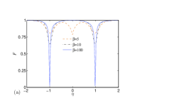
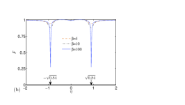
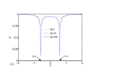
Figure 3: (Color online) $2$-D plots of mixed-state fidelity of finite-temperature thermal state of the non-Hermitian Ising model. We consider the cases with $N=10^{4}$ and field parameters (a) $\xi=0$, $\Delta\eta=\Delta\xi=0.01J^{-1}$, (b) $\xi=0.4$, $\Delta\eta=\Delta\xi=0.01J^{-1}$ and (c) $\xi=0.8$, $\Delta\eta=\Delta\xi=0.01J^{-1}$. Three curves represent the fidelities at various temperatures indicated in figures, respectively. It shows that the decay of fidelity for low temperature well indicates the critical point of the non-Hermitian Ising model. When the temperature increases, the decay of fidelity becomes less sharp, leading to boundary broadening of QPT.

IV Summary and discussion

In summary, we have shown that the QPT in a non-Hermitian Ising model has residual criticality at finite temperature, which can be described by the mixed-state fidelity in the context of biorthogonal bases. The successful extension of mixed-state fidelity to complex regime may be ascribed to the following two facts: At first, we happen to have an exact solvable non-Hermitian model, whose ground state is divided into several regions, or phases in the a complex-parameter plane. So far, this model is unique, while the QPT in most discovered non-Hermitian models is referred as the exceptional point. Secondly, the biorthogonal complete set is employed to formulate the density matrix of a thermal state. In this situation, we cannot give a general conclusion for other non-Hermitian systems, which should be investigated in the future.

Our study shows that quantum criticality in such a non-Hermitian system appears remarkably even at finite temperature. This paves the way for experimental detection of quantum criticality in complex-parameter plane. In experiment, there are several ways to realize the Hermitian Ising model, such as using trapped ions K ; Porras ; Wang ; Gong , an array of cavities Joshi ; Bardyn , atoms within a cavity Parkins , and Rydberg atoms in an optical lattice Tony1 ; K1 ; Bason ; Dudin . Recently, it was pointed that Tony2 , an imaginary transverse field may be implemented by optically pumping a qubit state into the auxiliary state.

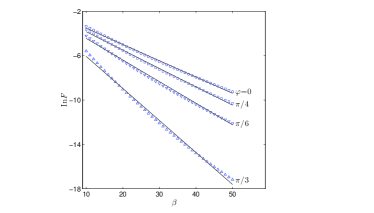
Figure 4: (Color online) Plots of $F$ as functions of temperature for several typical values of $\varphi$ and $N=10^{4}$, where $\beta$ is in the unit of $J^{-1}$. We fit the data with the functions in Eqs. (26) and (27).

*

Appendix A Exact solution of the $\mathcal{H}$

We consider the solution of the non-Hermitian Hamiltonian of Eq. (1). We start by taking the Jordan-Wigner transformation P.Jordan

$$\sigma_{j}^{+} = \prod\limits_{l<j}\left(1-2c_{l}^{{\dagger}}c_{l}\right)c_{j},$$ (28)

$$\sigma_{j}^{x} = 1-2c_{j}^{{\dagger}}c_{j},$$ (29)

$$\sigma_{j}^{z} = -\prod\limits_{l<j}\left(1-2c_{l}^{\dagger}c_{l}\right)\left(c_{j}+c_{j}^{\dagger}\right),$$ (30)

to replace the Pauli operators by the fermionic operators $c_{j}$. Likewise, the parity of the number of fermions

$$\Pi=\prod_{l=1}^{2N}\left(\sigma_{l}^{x}\right)=\left(-1\right)^{N_{p}}$$ (31)

is a conservative quantity, i.e., $\left[\mathcal{H},\Pi\right]=0$, where $N_{p}=\sum_{j=1}^{2N}c_{j}^{{\dagger}}c_{j}$. Then the Hamiltonian (1) can be rewritten as

$$\mathcal{H}=\sum_{\sigma=+,-}P_{\sigma}\mathcal{H}_{\sigma}P_{\sigma},$$ (32)

where

$$P_{\sigma}=\frac{1}{2}\left(1+\sigma\Pi\right)$$ (33)

is the projector on the subspaces with even ($\sigma=+$) and odd ($\sigma=-$) $N_{p}$. The Hamiltonian in each invariant subspace has the form

$$\mathcal{H}_{\sigma} = -J\sum\limits_{j=1}^{2N-1}\left(c_{j}^{{\dagger}}c_{j+1}+c_{j+1}^{{\dagger}}c_{j}+c_{j}^{{\dagger}}c_{j+1}^{{\dagger}}+c_{j+1}c_{j}\right)$$ (34)

$$+J\sigma\left(c_{2N}^{{\dagger}}c_{1}+c_{1}^{{\dagger}}c_{2N}+c_{2N}^{{\dagger}}c_{1}^{{\dagger}}+c_{1}c_{2N}\right)$$

$$-Jg_{j}\sum\limits_{j=1}^{2N-1}\left(1-2c_{j}^{\dagger}c_{j}\right)$$

taking the Fourier transformation

$$c_{j}=\frac{1}{\sqrt{N}}\sum\limits_{k_{\zeta}}e^{ik_{\zeta}j}\left\{\begin{array}[]{cc}\alpha_{k_{\zeta}},&\text{even }j\\ \beta_{k_{\zeta}},&\text{odd }j\end{array}\right.,$$ (35)

for the Hamiltonians $\mathcal{H}_{\sigma}$, we have

$$\mathcal{H}_{\sigma} = -J\sum_{k_{\sigma}}H_{k_{\sigma}}$$ (36)

$$H_{k_{\sigma}} = \left(e^{ik_{\sigma}}+1\right)\alpha_{k_{\sigma}}^{\dagger}\beta_{k_{\sigma}}+\left(e^{ik_{\sigma}}-1\right)\alpha_{k_{\sigma}}^{\dagger}\beta_{-k_{\sigma}}^{\dagger}+\mathrm{H.c.}$$ (37)

$$+2\eta-2\left(\eta+i\xi\right)\alpha_{k_{\sigma}}^{\dagger}\alpha_{k_{\sigma}}$$

$$-2\left(\eta-i\xi\right)\beta_{k_{\sigma}}^{{\dagger}}\beta_{k_{\sigma}}$$

where the momentum $k_{\sigma}$ are defined as $k_{+}=2\left(m+1/2\right)\pi/N$, $k_{-}=2m\pi/N$, $m=0,1,2,...,N-1$, respectively.

In this paper, we focus on the case with large $N$, in which the effect of $k_{+}-k_{-}$ can be neglected. In the following we will neglect the subscript $\sigma$ in $k_{\sigma}$. In order to obtain the eigen states in both subspaces with even and odd $N_{p}$, what we need is to diagonalize the Hamiltonian

$$h_{k}=H_{k}+H_{-k}$$ (38)

with

$$H_{k} = 2e^{ik/2}\cos\left(k/2\right)\alpha_{k}^{\dagger}\beta_{k}+i2e^{ik/2}\sin\left(k/2\right)\alpha_{k}^{\dagger}\beta_{-k}^{\dagger}+\mathrm{H.c.}$$ (39)

$$+2\eta-2\left(\eta+i\xi\right)\alpha_{k}^{\dagger}\alpha_{k}-2\left(\eta-i\xi\right)\beta_{k}^{{\dagger}}\beta_{k},$$

due to the fact $\left[h_{k},h_{k^{\prime}}\right]\propto 0$. This procedure is similar to introduce the Bogoliubov transformation for solving a simple transverse field Ising model. There are two $8$-dimensional invariant spaces for $h_{k}$, spanned by two sets of bases $\{\alpha_{\pm k}^{\dagger}\left|0\right\rangle$, $\beta_{\pm k}^{\dagger}\left|0\right\rangle$, $\alpha_{\pm k}^{\dagger}\alpha_{\mp k}^{\dagger}\beta_{\pm k}^{\dagger}\left|0\right\rangle$, $\beta_{\pm k}^{\dagger}\beta_{\mp k}^{\dagger}\alpha_{\pm k}^{\dagger}\left|0\right\rangle\}$ and $\{\left|0\right\rangle$, $\alpha_{\pm k}^{\dagger}\beta_{\mp k}^{\dagger}\left|0\right\rangle$, $\alpha_{\pm k}^{\dagger}\beta_{\pm k}^{\dagger}\left|0\right\rangle$, $\alpha_{k}^{\dagger}\alpha_{-k}^{\dagger}\left|0\right\rangle$, $\beta_{k}^{\dagger}\beta_{-k}^{\dagger}\left|0\right\rangle$, $\alpha_{k}^{\dagger}\beta_{k}^{\dagger}\alpha_{-k}^{\dagger}\beta_{-k}^{\dagger}\left|0\right\rangle\}$, involving odd and even numbers of fermions, respectively. Here $\left|0\right\rangle$ is the vacuum of fermion operator $c_{j}$, i.e., $c_{j}\left|0\right\rangle=0$. Fortunately, such two $8\times 8$ matrices can be diagonalized analytically in the form

$$h_{k}\overline{\left|n\right\rangle}_{k}=2\epsilon^{n}\left(k\right)\overline{\left|n\right\rangle}_{k},n\in\left[1,16\right],$$ (40)

where $\overline{\left|n\right\rangle}_{k}$ and $\epsilon^{n}\left(k\right)$ are listed in Eqs. (4)-(10), which can be used to construct the eigenstates and spectrum of the original Hamiltonian. By the same procedure, we can obtain the eigenstates of $\mathcal{H}^{{\dagger}}$.

- (1) S. Sachdev, Quantum Phase Transition (Cambridge University Press, Cambridge, 1999).
- (2) P. Zanardi, H. T. Quan, X. G. Wang, and C. P. Sun, Phys. Rev. A 75, 032109 (2007).
- (3) C. M. Bender, and S. Boettcher, Phys. Rev. Lett. 80, 5243 (1998).
- (4) C. M. Bender, S. Boettcher, and P. N. Meisinger, J. Math. Phys. 40, 2201 (1999).
- (5) P. Dorey, C. Dunning, and R. Tateo, J. Phys. A: Math. Gen. 34, L391 (2001); P. Dorey, C. Dunning, and R. Tateo, J. Phys. A: Math. Gen. 34, 5679 (2001).
- (6) C. M. Bender, D. C. Brody, and H. F. Jones, Phys. Rev. Lett. 89, 270401 (2002).
- (7) A. Mostafazadeh, J. Math. Phys. 43, 3944 (2002).
- (8) A. Mostafazadeh and A. Batal, J. Phys. A: Math. Gen. 37, 11645 (2004).
- (9) A. Mostafazadeh, J. Phys. A: Math. Gen. 36, 7081 (2003).
- (10) H. F. Jones, J. Phys. A: Math. Gen. 38, 1741 (2005).
- (11) A. Mostafazadeh, J. Math. Phys. 43, 2814 (2002).
- (12) C. Li, G. Zhang, X. Z. Zhang, and Z. Song, Phys. Rev. A 90, 012103 (2014).
- (13) P. Zanardi and N. Paunković, Phys. Rev. E 74, 031123 (2006); P. Zanardi, M. Cozzini, and P. Giorda, J. Stat. Mech. (2007) L02002; M. Cozzini, P. Giorda, and P. Zanardi, Phys. Rev. B 75, 014439 (2007); M. Cozzini, R. Ionicioiu, and P. Zanardi, Phys. Rev. B 76, 104420 (2007); P. Zanardi, P. Giorda, and M. Cozzini, Phys. Rev. lett. 99, 100603 (2007)
- (14) P. Buonsante and A. Vezzani, Phys. Rev. Lett. 98, 110601 (2007).
- (15) S. Chen, L. Wang, S. J. Gu, and Y. P. Wang, Phys. Rev. E 76, 061108 (2007).
- (16) M. F. Yang, Phys. Rev. B 76, 180403(R) (2007).
- (17) H. Q. Zhou and J. P. Barjaktarevič, J. Phys. A: Math. Theor. 41 (2008) 412001.
- (18) D. Schwandt, F. Alet, and S. Capponi, Phys. Rev. Lett. 103, 170501 (2009).
- (19) M. M. Rams and B. Damski, Phys. Rev. Lett. 106, 055701 (2011).
- (20) N. Paunković, P. D. Sacramento, P. Nogueira, V. R. Vieira, and V. K. Dugaev, Phys. Rev. A 77, 052302 (2008).
- (21) H. T. Quan and F. M. Cucchietti, Phys. Rev. E 79, 031101 (2009).
- (22) J. Sirker, Phys. Rev. Lett. 105, 117203 (2010).
- (23) K. Mølmer and A. Sørensen, Phys. Rev. Lett. 82, 1835 (1999).
- (24) D. Porras and J. I. Cirac, Phys. Rev. Lett. 92, 207901 (2004).
- (25) J.W. Britton, B. C. Sawyer, A. C. Keith, C.-C. J. Wang, J. K. Freericks, H. Uys, M. J. Biercuk, and J. J. Bollinger, Nature (London) 484, 489 (2012).
- (26) P. Richerme, Z. X. Gong, A. Lee, C. Senko, J. Smith, M. Foss-Feig, S. Michalakis, A. V. Gorshkov, and C. Monroe, Nature (London) 511, 198 (2014).
- (27) C. Joshi, F. Nissen, and J. Keeling, Phys. Rev. A 88, 063835 (2013).
- (28) C. E. Bardyn and A. İmamoğlu, Phys. Rev. Lett. 109, 253606 (2012).
- (29) S. Morrison and A. S. Parkins, Phys. Rev. Lett. 100, 040403 (2008).
- (30) T. E. Lee, S. Gopalakrishnan, and M. D. Lukin, Phys. Rev. Lett. 110, 257204 (2013).
- (31) I. Bouchoule and K. Mølmer, Phys. Rev. A 65, 041803 (2002).
- (32) M. Viteau, M. G. Bason, J. Radogostowicz, N. Malossi, D. Ciampini, O. Morsch, and E. Arimondo, Phys. Rev. Lett. 107, 060402 (2011).
- (33) L. Li, Y. O. Dudin, and A. Kuzmich, Nature (London) 498, 466 (2013).
- (34) T. E. Lee and C. K. Chan, Phys. Rev. X. 4, 041001 (2014).
- (35) P. Jordan and E. Wigner, Z. Physik 47, 631 (1928).