Determinantal structures in the O’Connell-Yor directed random polymer model

Abstract

We study the semi-discrete directed random polymer model introduced by O’Connell and Yor. We obtain a representation for the moment generating function of the polymer partition function in terms of a determinantal measure. This measure is an extension of the probability measure of the eigenvalues for the Gaussian Unitary Ensemble (GUE) in random matrix theory. To establish the relation, we introduce another determinantal measure on larger degrees of freedom and consider its few properties, from which the representation above follows immediately.

1 Introduction

In this paper we consider a directed random polymer model in random media in two (one discrete and one continuous) dimension introduced by O’Connell and Yor [59]. For $N$ independent one-dimensional standard Brownian motions $B_{j}(t),~{}j=1,\cdots,N$ and the parameter $\beta(>0)$ representing the inverse temperature, the polymer partition function is defined by

$$Z_{N}(t)=\int_{0<s_{1}<\cdots<s_{N-1}<t}e^{\beta\left(B_{1}(s_{1})+B_{2}(s_{1},s_{2})+\cdots+B_{N}(s_{N-1},t)\right)}ds_{1}\cdots ds_{N-1}.$$ (1.1)

Here $B_{j}(s,t)=B_{j}(t)-B_{j}(s),~{}j=2,\cdots,N$ for $s<t$ and $-B_{1}(s_{1})-B_{2}(s_{1},s_{2})-\cdots-B_{N}(s_{N-1},t)$ represents the energy of the polymer. In the last fifteen years much progress has been made on this O’Connell-Yor polymer model, by which we can access some explicit information about $Z_{N}(t)$ and the polymer free energy $F_{N}(t)=-\log(Z_{N}(t))/\beta$ [7, 10, 11, 36, 41, 45, 46, 47, 54, 57, 72]. The first breakthrough was made in the zero temperature $(\beta\rightarrow\infty)$ case. In this limit, $-F_{N}(t)$ becomes

$$f_{N}(t):=-\lim_{\beta\rightarrow\infty}F_{N}(t)=\max_{0<s_{1}<\cdots<s_{N-1}<t}\left(B_{1}(s_{1})+B_{2}(s_{1},s_{2})+\cdots+B_{N}(s_{N-1},t)\right)$$ (1.2)

where $-f_{N}(t)$ is the ground state energy. For $f_{N}(t)$, the following relation was established [7, 36]:

$$\text{Prob}\left(f_{N}(t)\leq s\right)=\int_{(-\infty,s]^{N}}\prod_{j=1}^{N}dx_{j}\cdot P_{\text{GUE}}(x_{1},\cdots,x_{N};t),$$ (1.3)

$$P_{\text{GUE}}(x_{1},\cdots,x_{N};t)=\prod_{j=1}^{N}\frac{e^{-x_{j}^{2}/2t}}{j!t^{j-1}\sqrt{2\pi t}}\cdot\prod_{1\leq j<k\leq N}(x_{k}-x_{j})^{2},$$ (1.4)

where $P_{\text{GUE}}(x_{1},\cdots,x_{N};t)$ is the probability density function of the eigenvalues in the Gaussian Unitary Ensemble (GUE) in random matrix theory [3, 35, 52]. This type of connection of the ground state energy of a directed polymer in random media with random matrix theory was first obtained for a directed random polymer model on a discrete space $\mathbb{Z}_{+}^{2}$ [42] by using the Robinson-Schensted-Knuth(RSK) correspondence. Eq. (1.3) can be regarded as its continuous analogue. Note that (1.4) is written in the form of a product of the Vandermonde determinant $\prod_{1\leq j<k\leq N}(x_{k}-x_{j})$. This feature implies that the $m$-point correlation function is described by an $m\times m$ determinant, i.e. the eigenvalues of the GUE are a typical example of the determinantal point processes [73]. In addition based on this fact and explicit expression of the correlation kernel, we can study the asymptotic behavior of $f_{N}(t)$ in the limit $N\rightarrow\infty$. In [7, 36], it has been shown that under a proper scaling, the limiting distribution of $f_{N}(t)$ becomes the GUE Tracy-Widom distribution [75].

In this paper, we provide a representation for a moment generating function of the polymer partition function (1.1) which holds for arbitrary $\beta(>0)$:

$$\mathbb{E}\left[\exp\left(-\frac{e^{-\beta u}Z_{N}(t)}{\beta^{2(N-1)}}\right)\right]=\int_{\mathbb{R}^{N}}\prod_{j=1}^{N}dx_{j}\,f_{F}(x_{j}-u)\cdot W(x_{1},\cdots,x_{N};t),$$ (1.5)

$$W(x_{1},\cdots,x_{N};t)=\prod_{j=1}^{N}\frac{1}{j!}\cdot\prod_{1\leq j<k\leq N}(x_{k}-x_{j})\cdot\det\left(\psi_{k-1}(x_{j};t)\right)_{j,k=1}^{N},$$ (1.6)

where $f_{F}(x)=1/(e^{\beta x}+1)$ is the Fermi distribution function and

$$\psi_{k}(x;t)=\frac{1}{2\pi}\int_{-\infty}^{\infty}dw\,e^{-iwx-w^{2}t/2}\frac{(iw)^{k}}{\Gamma\left(1+iw/\beta\right)^{N}}.$$ (1.7)

For more details see Definition 1 and Theorem 2 below. This is a simple generalization of (1.3) to the case of finite temperature. We easily find that it recovers (1.3) in the zero-temperature limit ($\beta\rightarrow\infty$). Note that the function $W(x_{1},\cdots,x_{N};t)$ is also written as a product of two determinants and thus retains the determinantal structure in (1.4).

In most cases, to find a finite temperature generalization of results for zero-temperature case is highly nontrivial and in fact often impossible. But for the O’Connell-Yor polymer model and a few related models, rich mathematical structures have been discovered for finite temperature and the studies on this topic entered a new stage [2, 10, 25, 37, 57, 61, 66, 67, 69, 68]. In [57], O’Connell found a connection to the quantum Toda lattice, and based on the developments in its studies and the geometric RSK correspondence, it was revealed that the law of the free energy $F_{N}(t)$ is expressed as

$$\text{Prob}\left(-F_{N}(t)+\frac{N-1}{\beta}\log\beta^{2}\leq s\right)=\int_{(-\infty,s]}dx_{1}\int_{\mathbb{R}^{N-1}}\prod_{j=2}^{N}dx_{j}\cdot m(x_{1},\cdots,x_{N};t).$$ (1.8)

Here the probability measure $m(x_{1},\cdots,x_{N};t)\prod_{j=1}^{N}dx_{j}$, which is called the Whittaker measure, is defined by the density function $m(x_{1},\cdots,x_{N};t)$ in terms of the Whittaker function $\Psi_{\lambda}(x_{1},\cdots,x_{N})$ (for the definition, see [57]) and the Sklyanin measure $s_{N}(\lambda)d\lambda$ (see (2.10) below) as follows,

$$m(x_{1},\cdots,x_{N};t)=\Psi_{0}(\beta x_{1},\cdots,\beta x_{N})\int_{(i\mathbb{R})^{N}}d\lambda\,\Psi_{-\lambda/\beta}(\beta x_{1},\cdots,\beta x_{N})e^{\sum_{j=1}^{N}\lambda_{j}^{2}t/2}s_{N}(\lambda/\beta),$$ (1.9)

where $\lambda$ represents $(\lambda_{1},\cdots,\lambda_{N})$. In contrast to (1.4), the density function (1.9) is not known to be expressed as a product of determinants and the process associated with (1.9) does not seem to be determinantal. Nevertheless some determinantal formulas for the O’Connell-Yor polymer have been found: First in [57], O’Connell showed a determinantal representation for the moment generating function (LHS of (1.5)) in terms of the Sklyanin measure. (See (2.9) below.) Next in [10], Borodin and Corwin obtained a Fredholm determinant representation for the same moment generating function (see (4.23) below). A direct proof of the equivalence between the two determinantal expressions was given in [13]. In [10], by considering its continuous limit, the authors also obtained an explicit representation of the free energy distribution for the directed random polymer in two continuous dimension described by stochastic heat equation (SHE) [10, 11]. The distribution in this limit, which describes the universal crossover between the Kardar-Parisi-Zhang (KPZ) and the Edwards-Wilkinson universality class, was first obtained in [2, 66, 67, 69, 68] and can be interpreted also as the height distribution for the KPZ equation [44]. Furthermore in [10], they consider not only the O’Connell-Yor model but a class of stochastic processes having the similar Fredholm determinant expressions, the Macdonald processes, the probability measures on a sequence of partitions which are written in terms of the Macdonald symmetric functions and include the Whittaker measure defined by (1.8) as a limiting case.

The purpose of this paper is to investigate further the mechanism of appearance of such determinantal structures and (1.5) is the central formula in our study. Although $W(x_{1},\cdots,x_{N};t)\prod_{j=1}^{N}dx_{j}$ defined by (1.6) is not a probability measure but a signed measure except when $\beta\rightarrow\infty$, a remarkable feature of this measure is that it is determinantal for arbitrary $\beta$ contrary to the Whittaker measure (1.9). This determinantal structure allows us to use the conventional techniques developed in the random matrix theory and thus from the relation we readily get a Fredholm determinant representation with a kernel using biorthogonal functions which is regarded as a generalization of the kernel with the Hermite polynomials for the GUE. In (1.6), the parameter $\beta$, which originally represents the inverse temperature in the polymer model appears in the Fermi distribution function $f_{F}(x-u)$ with the chemical potential $u$ as well as $\psi_{k}(x;t)$ (1.7) in RHS. This fact with the determinantal structure suggests that the RHS might have something to do with the free Fermions at a finite temperature. Related to this, a curious relation of the height of the KPZ equation with Fermions has been discussed in [28].

For establishing the relation, we introduce a measure on a larger space $\mathbb{R}^{N(N+1)/2}$. By integrating the measure in two different ways, we get its two marginal weights. In one formula appears a determinant which solves the $N$ dimensional diffusion equation with some condition (see (2.11), (3.6), and (3.7)) and the other one with a symmetrization is exactly the RHS of (1.5). The relation (1.5) follows immediately from the equivalence of these two expressions. Our approach is similar to the one by Warren [78] for getting the relation (1.3). Actually in the zero-temperature limit $\beta\rightarrow\infty$, we see that the integration of the measure is written in terms of the probability measure introduced in [78], which describes the positions of the reflected Brownian particles on the Gelfand-Tsetlin cone. Note that the Macdonald processes (especially the Whittaker process in our case) [10] are also another generalizations of [78]. Although the Whittaker process has rich integrable properties, they do not inherit the determinantal structure of [78]. On the other hand, our measure is described without using the Whittaker functions and keeps the determinantal structure. Furthermore combining (1.5) with the fact that the quantity can be rewritten as the Fredholm determinant found in [10] (Corollary 13 and Proposition 15 below), our approach can be considered as another proof of the equivalence between (4.23) and (2.9) in [13]. One feature of our proof is to bring to light the larger determinantal structure behind the two relations.

This paper is organized as follows. In the next section, after stating the definition of a determinantal measure, we give our main result, Theorem 2 and its proof. The proof consists of two major steps: we first introduce in Lemma 3 a determinantal representation for the moment generating function which is a deformed version of the representation (2.9) in [57]. Next we introduce another determinantal measure on larger space $\mathbb{R}^{N(N+1)/2}$ and then we find two relations about its integrations which play a key role in deriving our main result. In Sec. 3 we show that this approach can be considered as an extension of the one in [78]. In Sec.4., we consider the Fredholm determinant formula with biorthogonal kernel obtained by applying conventional random matrix techniques to our main result. The scaling limit to the KPZ equation is discussed in Sec.5. We check that our kernel goes to the one obtained in the studies of the KPZ equation. A concluding remark is given in the last section.

2 Main result

In this section, we introduce a measure $W(x_{1},\cdots,x_{N};t)\prod_{j=1}^{N}dx_{j}$ (1.6), state our main result and give its proof.

2.1 Definition and result

Definition 1.

Let $\psi_{k}(x;t),~{}k=1,2,\cdots$ be

$$\psi_{k}(x;t)=\frac{1}{2\pi}\int_{-\infty}^{\infty}dw\,e^{-iwx-w^{2}t/2}\frac{(iw)^{k}}{\Gamma\left(1+iw/\beta\right)^{N}}.$$ (2.1)

For $(x_{1},\cdots,x_{N})\in\mathbb{R}^{N}$, a function $W(x_{1},\cdots,x_{N};t)$ is defined by

$$W(x_{1},\cdots,x_{N};t)=\prod_{j=1}^{N}\frac{1}{j!}\cdot\prod_{1\leq l<m\leq N}(x_{m}-x_{l})\cdot\det\left(\psi_{j-1}(x_{k};t)\right)_{j,k=1}^{N}.$$ (2.2)

Remark. We find that $W(x_{1},\cdots,x_{N};t)$ is a real function on $\mathbb{R}^{N},$ since by definition $\psi_{k}(x;t)$ is real for any $k=0,1,2,\cdots,N-1,\beta>0$ and $t>0$. But in general, the positivity of this measure is not guaranteed. For example $\psi_{0}(x;t)$ shows a damped oscillation and can take a negative value for some $x$. Thus at least for the case $N=1$, $W(x,t)=\psi_{0}(x;t)$ can be negative.

We discuss the zero-temperature limit $\beta\rightarrow\infty$ of $W(x_{1},\cdots,x_{N};t)$. Noting $\Gamma(1)=1$, we see

$$\lim_{\beta\rightarrow\infty}\psi_{k}(x;t)=\frac{1}{2\pi}\int_{-\infty}^{\infty}dw\,e^{-iwx-w^{2}t/2}(iw)^{k}=\frac{e^{-x^{2}/2t}}{\sqrt{2\pi t}}\left(\frac{1}{2t}\right)^{\frac{k}{2}}H_{k}\left(\frac{x}{\sqrt{2t}}\right),$$ (2.3)

where we used the integral representations of the $n$th order Hermite polynomial $H_{n}(x)$ (see e.g. Section 6.1 in [5]),

$$H_{n}(x)=\frac{(-2i)^{n}}{\sqrt{\pi}}\int_{-\infty}^{\infty}du\,u^{n}e^{-(u-ix)^{2}}$$ (2.4)

Note that $(t/2)^{k/2}H_{k}(x/\sqrt{2t})$ is a monic polynomial (i.e. the coefficient of the highest degree is 1) and

$$\lim_{\beta\rightarrow\infty}\det\left(\psi_{k-1}(x_{j};t)\right)_{j,k=1}^{N}=\prod_{j=1}^{N}\frac{e^{-x_{j}^{2}/2t}}{t^{j-1}\sqrt{2\pi t}}\cdot\prod_{1\leq j<k\leq N}(x_{k}-x_{j}).$$ (2.5)

Thus we find

$$\lim_{\beta\rightarrow\infty}W(x_{1},\cdots,x_{N};t)=P_{\text{GUE}}(x_{1},\cdots,x_{N};t),$$ (2.6)

where $P_{\text{GUE}}(x_{1},\cdots,x_{N};t)$ is defined by (1.4). The function $W(x_{1},\cdots,x_{N};t)$ can be regarded as a deformation of  (1.4) which keeps its determinantal structure.

In this paper, we provide a determinantal representation for the moment generating function of the polymer partition function (1.1) in terms of the function (2.2).

Theorem 2.

$$\mathbb{E}\left(e^{-\frac{e^{-\beta u}Z_{N}(t)}{\beta^{2(N-1)}}}\right)=\int_{\mathbb{R}^{N}}\prod_{j=1}^{N}dx_{j}\,f_{F}(x_{j}-u)\cdot W(x_{1},\cdots,x_{N};t)$$ (2.7)

where $f_{F}(x)=1/(e^{\beta x}+1)$ is the Fermi distribution function.

By (1.2), (2.6) and the simple facts

$$\lim_{\beta\rightarrow\infty}e^{-e^{\beta x}}=\lim_{\beta\rightarrow x}f_{F}(x)=\Theta(-x),$$ (2.8)

we find that the zero temperature limit of (2.7) becomes (1.3).

Because of the determinantal structure of $W(x_{1},\cdots,x_{N};t)$, we can get the Fredholm determinant representation for the moment generating function by using the techniques in random matrix theory. Recently another Fredholm determinant representation has been given based on properties of Macdonald difference operators [10]. The equivalence between them will be shown in Sec. 4.

2.2 Proof

Here we provide a proof of Theorem 2. Our starting point is the representation for the moment generating function given in [57]:

$$\mathbb{E}\left(e^{-\frac{e^{-\beta u}Z_{N}(t)}{\beta^{2(N-1)}}}\right)=\int_{(i\mathbb{R}-\epsilon)^{N}}\prod_{j=1}^{N}\frac{d\lambda_{j}}{\beta}e^{-u\lambda_{j}+\lambda_{j}^{2}t/2}\Gamma\left(-\frac{\lambda_{j}}{\beta}\right)^{N}\cdot s_{N}\left(\frac{\lambda}{\beta}\right),$$ (2.9)

where $0<\epsilon<\beta$ and $s_{N}(\lambda)d\lambda$ is the Sklyanin measure defined by

$$s_{N}(\lambda)=\frac{1}{(2\pi i)^{N}N!}\prod_{i<j}\frac{\sin\pi(\lambda_{i}-\lambda_{j})}{\pi}\prod_{i>j}\left(\lambda_{i}-\lambda_{j}\right).$$ (2.10)

This relation was obtained by using the properties of the Whittaker functions [22, 74] and the Whittaker measure (4.21).

Lemma 3.

$$\mathbb{E}\left(e^{-\frac{e^{-\beta u}Z_{N}(t)}{\beta^{2(N-1)}}}\right)=\int_{\mathbb{R}^{N}}\prod_{\ell=1}^{N}dx_{\ell}f_{F}(x_{\ell}-u)\cdot G(x_{1},\cdots,x_{N};t)$$ (2.11)

where $f_{F}(x)$ is defined below (4.17) and

$$G(x_{1},\cdots,x_{N};t)=\det\left(F_{jk}(x_{N-j+1};t)\right)_{j,k=1}^{N},$$ (2.12)

$$F_{jk}(x;t)=\int_{i\mathbb{R}-\epsilon}\frac{d\lambda}{2\pi i}\frac{e^{-\lambda x+\lambda^{2}t/2}}{\Gamma\left(\frac{\lambda}{\beta}+1\right)^{N}}\left(\frac{\pi}{\beta}\cot\frac{\pi\lambda}{\beta}\right)^{j-1}\lambda^{k-1}$$ (2.13)

with $0<\epsilon<\beta$.

We will discuss an interpretation of (2.12) in the next section. In this definition, we have arranged $x_{i}$’s in the reversed order so as to relate (3.17), the zero-temperature limit of (2.12), to the stochastic processes defined later in (3.20).

Proof. Noting the relation

$$~{}\prod_{1\leq i<j\leq N}{\sin(x_{i}-x_{j})}=\prod_{1\leq i<j\leq N}\sin x_{i}\sin x_{j}\left(\cot x_{j}-\cot x_{i}\right)$$

$$=\prod_{j=1}^{N}\sin^{N-1}x_{j}\cdot\prod_{1\leq k<\ell\leq N}\left(\cot x_{\ell}-\cot x_{k}\right)=\prod_{j=1}^{N}\sin^{N-1}x_{j}\cdot\det\left(\cot^{\ell-1}x_{k}\right)_{k,\ell=1}^{N},$$ (2.14)

we rewrite RHS of (2.9) as

$$~{}~{}\int_{(i\mathbb{R}-\epsilon)^{N}}\prod_{j=1}^{N}\frac{d\lambda_{j}}{\beta}e^{-u\lambda_{j}+\lambda_{j}^{2}t/2}\Gamma\left(-\frac{\lambda_{j}}{\beta}\right)^{N}\cdot s_{N}\left(\frac{\lambda}{\beta}\right)$$

$$=\frac{1}{N!}\int_{(i\mathbb{R}-\epsilon)^{N}}\prod_{j=1}^{N}\frac{d\lambda_{j}}{2\pi i\beta}e^{-u\lambda_{j}+\lambda_{j}^{2}t/2}\Gamma\left(-\frac{\lambda_{j}}{\beta}\right)^{N}\left(\frac{\sin\frac{\pi}{\beta}\lambda_{j}}{\pi}\right)^{N-1}$$

$$\hskip 51.21504pt\times\det\left(\left(\frac{\pi}{\beta}\cot\frac{\pi}{\beta}\lambda_{j}\right)^{k-1}\right)_{j,k=1}^{N}\det\left({\lambda_{j}}^{k-1}\right)_{j,k=1}^{N}$$

$$=\det\left(\int_{i\mathbb{R}-\epsilon}\frac{d\lambda}{2\pi i\beta}e^{-u\lambda+\lambda^{2}t/2}\Gamma\left(-\frac{\lambda}{\beta}\right)^{N}\left(\frac{\sin\frac{\pi}{\beta}\lambda}{\pi}\right)^{N-1}\left(\frac{\pi}{\beta}\cot\frac{\pi}{\beta}\lambda\right)^{j-1}\lambda^{k-1}\right)_{j,k=1}^{N}$$ (2.15)

where in the last equality, we used the Andréief identity (also known as the Cauchy-Binet identity) [4]: For the functions $g_{j}(x),~{}h_{j}(x)$, $j=1,2,\dots,N,$ such that all integrations below are well-defined, we have

$$\frac{1}{N!}\int_{\mathbb{R}^{N}}\prod_{j=1}^{N}dx_{j}\cdot\det\left(g_{k}(x_{j})\right)_{j,k=1}^{N}\det\left(h_{k}(x_{j})\right)_{j,k=1}^{N}=\det\left(\int_{\mathbb{R}}dxg_{j}(x)h_{k}(x)\right)_{j,k=1}^{N}.$$ (2.16)

We notice that the factor $e^{-u\lambda}\Gamma(-\lambda/\beta)^{N}({\sin(\pi\lambda/\beta)}/{\pi})^{N-1}$in (2.15) can be written as

$$e^{-u\lambda}\Gamma\left(-\frac{\lambda}{\beta}\right)^{N}\left(\frac{\sin\frac{\pi}{\beta}\lambda}{\pi}\right)^{N-1} =\frac{(-1)^{N-1}}{\Gamma\left(1+\frac{\lambda}{\beta}\right)^{N}}\frac{\pi e^{-u\lambda}}{-\sin\frac{\pi}{\beta}\lambda}$$

$$=\frac{(-1)^{N-1}}{\Gamma\left(1+\frac{\lambda}{\beta}\right)^{N}}\int_{-\infty}^{\infty}\beta\frac{e^{-x\lambda}}{e^{\beta(x-u)}+1}dx$$ (2.17)

where we used the reflection formula for the Gamma function and the relation (4.31). From (2.15) and (2.17), we arrive at the desired expression (2.11). ∎

From (2.11), we see that for the derivation of our main result (2.7), it is sufficient to prove the relation

$$\int_{\mathbb{R}^{N}}\prod_{\ell=1}^{N}dx_{\ell}f_{F}(x_{\ell}-u)\cdot G(x_{1},\cdots,x_{N};t)=\int_{\mathbb{R}^{N}}\prod_{j=1}^{N}dx_{j}\,f_{F}(x_{j}-u)\cdot W(x_{1},\cdots,x_{N};t).$$ (2.18)

where $f_{F}(x)$ is defined below (2.7) and $W(x_{1},\cdots,x_{N};t)$ is given in Definition 1. Note that this is a relation for the integrated values on $\mathbb{R}^{N}$. To establish this we introduce a measure on the larger space $\mathbb{R}^{N(N+1)/2}$.

Definition 4.

Let $\underline{x}_{k}$ be an array $(x^{(1)},\cdots,x^{(k)})$ where $x^{(j)}=(x^{(j)}_{1},\cdots,x^{(j)}_{j})\in\mathbb{R}^{j}$ and $d\underline{x}_{k}=\prod_{j=1}^{k}\prod_{i=1}^{j}dx^{(j)}_{i}$. We define a measure $R_{u}(\underline{x}_{N};t)d\underline{x}_{N}$ by

$$R_{u}(\underline{x}_{N};t)=\prod_{1\leq i\leq j\leq N}f_{i}(x^{(j)}_{i}-x^{(j-1)}_{i-1})\cdot\det\left(F_{1i}(x^{(N)}_{j};t)\right)_{i,j=1}^{N}.$$ (2.19)

Here $x^{(j-1)}_{0}=u$, $F_{1j}(x;t)$ is given by $F_{ij}(x;t)$ (2.13) with $i=1$ and $f_{i}(x),i=1,2,\cdots$ is defined by using the Fermi and Bose distribution functions, $f_{F}(x):=1/(e^{\beta x}+1)$ and $f_{B}(x):=1/(e^{\beta x}-1)$ respectively as follows.

$$f_{i}(x)=\begin{cases}f_{F}(x),&i=1,\\ f_{B}(x),&i\geq 2.\end{cases}$$ (2.20)

Remark. The reason why both the Bose and Fermi distributions appear in our approach is not clear. The interrelations between them (see (2.28)-(2.30) below) will play an important role in the following discussions.

As in Fig 1. we usually represent the array $\underline{x}_{N}$ graphically in the triangular shape. Although no ordering is imposed on $\underline{x}_{N}$, in the zero-temperature limit, $R_{u}(\underline{x}_{N};t)$ has the support on the ordered arrays as in Fig. 1 (a) (see (3.34)). Fig. 1 (b) represents the other ordered array called the Gelfand-Tsetlin pattern (see (3.23)).

Figure 1: Triangular arrays ($k=3$) (a) an element of $V_{k}$ (3.34) (b) The Gelfand-Tsetrlin pattern (an element of (3.23))

As discussed later we will find that the moment generating function of the O’Connell-Yor polymer model is expressed as the integration of this measure $R_{u}(\underline{x}_{N};t)$ over $\mathbb{R}^{N(N+1)/2}$. We have other choices for the definition of $R_{u}(\underline{x}_{N};t)$ which give the same integration value. One example is

$$\bar{R}_{u}(\underline{x}_{N};t)=\prod_{\ell=1}^{N}\frac{1}{\ell!}\det\left(f_{i}(x^{(\ell)}_{j}-x^{(\ell-1)}_{i-1})\right)_{i,j=1}^{\ell}\cdot\det\left(F_{1i}(x^{(N)}_{j};t)\right)_{i,j=1}^{N}.$$ (2.21)

This comes form the following consideration. Let $f_{\text{sym}}(\underline{x}_{N})$ be a function which is symmetric under permutations of $x^{(j)}_{1},\cdots,x^{(j)}_{j}$ for each $j\in\{1,2,\cdots,N\}$. Then we see that $R_{u}(\underline{x}_{N};t)$ (2.19) and $\bar{R}_{u}(\underline{x}_{N};t)$ have the same integration value:

$$\int_{\mathbb{R}^{N(N+1)/2}}d\underline{x}_{N}f_{\rm{sym}}(\underline{x}_{N})R_{u}(\underline{x}_{N};t)=\int_{\mathbb{R}^{N(N+1)/2}}d\underline{x}_{N}f_{\rm{sym}}(\underline{x}_{N})\bar{R}_{u}(\underline{x}_{N};t).$$ (2.22)

It can be shown as follows. From the symmetry of $f_{\text{sym}}(\underline{x}_{N})$, LHS of the equation above becomes

$$\int_{\mathbb{R}^{N(N+1)/2}}d\underline{x}_{N}f_{\rm{sym}}(\underline{x}_{N})R_{u}(\underline{x}_{N};t)=\int_{\mathbb{R}^{N(N+1)/2}}d\underline{x}_{N}f_{\rm{sym}}(\underline{x}_{N})\tilde{R}_{u}(\underline{x}_{N};t).$$ (2.23)

Here $\tilde{R}_{u}(\underline{x}_{N};t)$ is defined by

$$\tilde{R}_{u}(\underline{x}_{N};t)=\prod_{\ell=1}^{N}\frac{1}{\ell!}\sum_{\sigma^{(j)}\in S_{j},~{}j=1,\cdots,N}R_{u}\left(\underline{x}_{N}^{\sigma};t\right),$$ (2.24)

where $S_{j}$ is the permutation of $1,2,\cdots,j$ and $\underline{x}_{N}^{\sigma}$ denotes $(x^{\sigma^{(1)}},\cdots,x^{\sigma^{(N)}})$ with $x^{\sigma^{(j)}}=(x^{(j)}_{\sigma^{(j)}(1)},\cdots,x^{(j)}_{\sigma^{(j)}(j)})$. We easily find the equivalence $\tilde{R}_{u}(\underline{x}_{N};t)=\bar{R}_{u}(\underline{x}_{N};t)$. Note that

$$~{}R_{u}(\underline{x}_{N}^{\sigma};t)=\prod_{1\leq i\leq j\leq N}f_{i}\left(x^{(j)}_{\sigma^{(j)}(i)}-x^{(j-1)}_{\sigma^{(j-1)}(i-1)}\right)\cdot\det\left(F_{1i}(x^{(N)}_{\sigma^{(N)}(j)};t)\right)_{i,j=1}^{N}$$

$$={\rm{sgn}}\sigma^{(N)}\prod_{j=1}^{N}\prod_{i=1}^{j}f_{i}\left(x^{(j)}_{\sigma^{(j)}(i)}-x^{(j-1)}_{\sigma^{(j-1)}(i-1)}\right)\cdot\det\left(F_{1i}(x^{(N)}_{j};t)\right)_{i,j=1}^{N}$$

$$=\prod_{j=1}^{N}{\rm{sgn}}\tau^{(j)}\prod_{i=1}^{j}f_{i}\left(x^{(j)}_{\tau^{(j)}(i)}-x^{(j-1)}_{i-1}\right)\cdot\det\left(F_{1i}(x^{(N)}_{j};t)\right)_{i,j=1}^{N}.$$ (2.25)

Here in the last equality, $\tau^{(j)}\in S_{j},~{}j=1,2,\cdots,N$ is defined by using $\sigma^{(j-1)}$ and $\sigma^{(j)}$ as $\sigma^{(j-1)}\tau^{(j)}(k)=\sigma^{(j)}(k),~{}k=1,\cdots,j$, where we regard $\sigma^{(j-1)}$ as an element of $S_{j}$ with $\sigma^{(j-1)}(j)=j$. Further in the last equality we used $\sigma^{(N)}=\prod_{j=1}^{N}\tau^{(j)}$. Substituting (2.25) into (2.24) and using the definition of the determinant, we have $\tilde{R}_{u}(\underline{x}_{N};t)=\bar{R}_{u}(\underline{x}_{N};t)$.

The function $\bar{R}_{u}(\underline{x}_{N};t)$ (2.21) has a similar determinantal structure to the Schur process [60]. The Schur process is a probability measure on the sequence of partitions $\{\lambda^{(j)}\}_{j=1,\cdots,N},$ where $\lambda^{(j)}:=\{(\lambda^{(j)}_{1},\cdots,\lambda^{(j)}_{j})|\lambda^{(j)}_{i}\in\mathbb{Z},~{}\lambda^{(j)}_{1}\geq\cdots\geq\lambda^{(j)}_{j}\geq 0\}$, described as products of the skew Schur functions $s_{\lambda/\mu}(x_{1},\cdots,x_{n})$. For the ascending case (see Definition 2.7 in [10]), the probability measure is expressed as

$$\prod_{i,j=1}^{N}\frac{1}{1-a_{i}b_{j}}\cdot\prod_{k=1}^{N}s_{\lambda^{(k)}/\lambda^{(k-1)}}(a_{k})\cdot s_{\lambda^{(N)}}(b_{1},\cdots,b_{N}),$$ (2.26)

where $a_{j},~{}b_{j},~{}j=1,\cdots,N$ are positive variables. We note that $s_{\lambda^{(k)}/\lambda^{(k-1)}}(a_{k})$ is expressed as a $k$th order determinant and $s_{\lambda^{(N)}}(b_{1},\cdots,b_{N})$ as a $N$th order determinant by the Jacobi-Trudi identity [50],

$$s_{\lambda/\mu}(x_{1},\cdots,x_{n})=\det\left(h_{\lambda_{i}-\mu_{j}+j-i}(x_{1},\cdots,x_{n})\right)_{i,j=1}^{\ell(\lambda)},$$ (2.27)

where $h_{k}(x_{1},\cdots,x_{n})$ is a complete symmetric polynomial with degree $k$ and $\ell(\lambda)$ is the length of the partition $\lambda$. Thus (2.21) and (2.26) have a common structure of $N$ products of determinants with increasing size times an $N$th order determinant.

In the following we provide the relations about two marginals of $R_{u}(\underline{x}_{N};t)$ (2.19), from which (2.18) immediately follows. For this purpose, we give two formulas for $f_{F}(x)$ and $f_{B}(x)$ (2.20). First we define a multiple convolution $g^{*(m)}f(x)~{}m=0,1,2,\cdots$ for a functions $f(x)$ on $\mathbb{R}$ and an integral operator $g$ with the kernel $g(x-y)$ as

$$g^{*(0)}f(x)=f(x),~{}g^{*(k)}f(x)=\int_{-\infty}^{\infty}dy\,g(x-y)g^{*(k-1)}f(y),~{}k=1,2,\cdots.$$ (2.28)

Using this definition, the formulas are written as follows:

Lemma 5.

We regard all integrations below as the Cauchy principal values. For $\beta>0$, $a\in\mathbb{C}$ with $-\beta<\text{Re~{}}a<0$ and $m=0,1,2,\cdots$, we have

$$f^{*(m)}_{B}e^{ax}=\left(\frac{\pi}{\beta}\cot\left(\frac{\pi a}{\beta}\right)\right)^{m}e^{ax},$$ (2.29)

$$f^{*(m)}_{B}f_{F}(x)=q_{m}(x)f_{F}(x),$$ (2.30)

where $q_{m}(x)$ is an $m$th order polynomial with the coefficient of the highest degree being $1/m!$.

A proof of this lemma will be given in Appendix A. The polynomial $q_{m}(x)$ in (2.30) is defined inductively by (A.11)-(A.13). But in our later discussion we will not use its explicit form.

From (2.13) and (2.29), we readily obtain for $m=0,1,2\cdots$,

$$\tilde{f}_{B}^{*(m)}F_{jk}\left(x;t\right)=F_{j+m,k}(x;t),$$ (2.31)

where we define $\tilde{f}_{B}(x):=f_{B}(-x)$.

Using (2.30) and (2.31), we obtain the following relations.

Theorem 6.

Let the measures $dA_{1}$ and $dA_{2}$ be

$$dA_{1}=\prod_{2\leq i\leq j\leq N}dx^{(j)}_{i},~{}dA_{2}=\prod_{1\leq i\leq j\leq N-1}dx^{(j)}_{i}.$$ (2.32)

Then we have

$$\int_{\mathbb{R}^{N(N-1)/2}}dA_{1}R_{u}(\underline{x}_{N};t)=G(x^{(1)}_{1},\cdots,x^{(N)}_{1};t)\prod_{j=1}^{N}f_{F}(x^{(j)}_{1}-u),$$ (2.33)

$$\int_{\mathbb{R}^{N(N-1)/2}}dA_{2}R_{u}(\underline{x}_{N};t)=\bar{W}(x^{(N)}_{1},\cdots,x^{(N)}_{N};t)\prod_{j=1}^{N}f_{F}(x^{(N)}_{j}-u).$$ (2.34)

Here $G(x^{(1)}_{1},\cdots,x^{(N)}_{1};t)$ is defined by (2.12) and

$$\bar{W}(x^{(N)}_{1},\cdots,x^{(N)}_{N};t)=\prod_{j=1}^{N-1}q_{j}\left(x^{(N)}_{j+1}-u\right)\cdot\det\left(F_{1j}\left(x^{(N)}_{k};t\right)\right)_{j,k=1}^{N},$$ (2.35)

where $q_{j}(x)$ is defined below (2.30).

We easily see that (2.18) can be obtained from these relations (2.33) and (2.34): Integrating the both hand sides of them over the remaining degrees of freedom ($(x^{(1)}_{1},\cdots,x^{(N)}_{1})$ for (2.33) and $(x^{(N)}_{1},\cdots,x^{(N)}_{N})$ for (2.34)), we get two different expression about the integrated value of $R_{u}(\underline{x}_{N};t)$

$$\int_{\mathbb{R}^{N(N+1)/2}}d\underline{x}_{N}R_{u}(\underline{x}_{N};t)=\int_{\mathbb{R}^{N}}\prod_{j=1}^{N}dx^{(j)}_{1}f_{F}(x^{(j)}_{1}-u)\cdot G(x^{(1)}_{1},\cdots,x^{(N)}_{1};t)$$ (2.36)

$$\int_{\mathbb{R}^{N(N+1)/2}}d\underline{x}_{N}R_{u}(\underline{x}_{N};t)=\int_{\mathbb{R}^{N}}\prod_{j=1}^{N}dx^{(N)}_{j}f_{F}(x^{(N)}_{j}-u)\cdot\bar{W}(x^{(N)}_{1},\cdots,x^{(N)}_{N};t).$$ (2.37)

where $d\underline{x}_{N}=\prod_{1\leq i\leq j\leq N}x^{(j)}_{i}$. RHS of the second relation is further rewritten as

$$\int_{\mathbb{R}^{N}}\prod_{j=1}^{N}dx^{(j)}_{1}f_{F}(x^{(j)}_{1}-u)\cdot\frac{1}{N!}\sum_{\sigma^{(N)}\in S_{N}}\bar{W}(x_{\sigma^{(N)}(1)},\cdots,x_{\sigma^{(N)}(N)};t),$$ (2.38)

and the symmetrized $\bar{W}(x_{1},\cdots,x_{N};t)$ in this equation is nothing but $W(x^{(N)}_{1},\cdots,x^{(N)}_{1};t)$ (2.2) since

$$\frac{1}{N!}\sum_{\sigma^{(N)\in S_{N}}}\bar{W}(x_{\sigma^{(N)}(1)},\cdots,x_{\sigma^{(N)}(N)};t) =\frac{1}{N!}\cdot\det\left(q_{j-1}(x^{(N)}_{k})\right)_{j,k=1}^{N}\det\left(F_{1j}(x^{(N)}_{k};t)\right)_{j,k=1}^{N}$$

$$=W(x^{(N)}_{1},\cdots,x^{(N)}_{N};t).$$ (2.39)

Here in the second equality we used the fact that $q_{j}(x)$ is a $j$th order polynomial with the coefficient of the highest degree being $1/j!$ and $F_{1j}(x;t)=\psi_{j}(x;t)$.

Proof of Theorem 6. First we derive (2.33). By the definition of (2.19), LHS of (2.33) becomes

$$\prod_{j=1}^{N}f_{F}(x^{(j)}_{1}-u)\cdot\det\left(\tilde{f}_{B}^{*(k-1)}F_{1j}\left(x^{(N-k+1)}_{1};t\right)\right)_{j,k=1}^{N}.$$ (2.40)

Here $\tilde{f}_{B}(x)$ is defined below (2.31). Applying (2.31) to this equation we obtain (2.33).

Next we derive (2.34). We see that the factor $dA_{2}\prod_{1\leq i\leq j\leq N}f_{i}(x^{(j)}_{i}-x^{(j-1)}_{i-1})$ in $R_{u}(\underline{x_{N}};t)$ (2.19) can be decomposed to

$$dA_{2}\prod_{1\leq i\leq j\leq N}f_{i}\left(x^{(j)}_{i}-x^{(j-1)}_{i-1}\right)=\prod_{k=1}^{N-1}\left(\prod_{i=1}^{N-k}dx^{(i+k-1)}_{i}\cdot\prod_{j=1}^{N-k+1}f_{j}\left(x^{(j+k-1)}_{j}-x^{(j+k-2)}_{j-1}\right)\right),$$ (2.41)

and from (2.30) the integration of the factor for each $k$ is represented as

$$\int_{\mathbb{R}^{N-k}}\prod_{1\leq i\leq N-k}dx^{(i+k-1)}_{i}\prod_{j=1}^{N-k+1}f_{j}(x^{(j+k-1)}_{i}-x^{(j+k-2)}_{j-1})=f^{*(N-k)}_{B}f_{F}(x^{(N)}_{N-k+1}-u)$$

$$=q_{N-k}(x^{(N)}_{N-k+1}-u)f_{F}(x^{(N)}_{N-k+1}-u)$$ (2.42)

where $q_{m}(x)$ is given in (2.30). Eq. (2.34) follows immediately from this relation. ∎

3 Dynamics of the two marginals

The purpose of this section is to have a better understanding of the two quantities, $W(x_{1},\cdots,x_{N};t)$ (2.2) and $G(x_{1},\cdots,x_{N};t)$ (2.12), which arose as partially integrated quantities of $R_{u}(\underline{x}_{N};t)$ (2.19) in Theorem 6 (for $W$ a symmetrization is also necessary, see (2.39)). We will first consider the evolution equations of these two quantities. Next we will see that the zero-temperature limit of the equation for $W(x_{1},\cdots,x_{N};t)$ is nothing but the evolution equation for the Brownian particles with reflection interaction while $W(x_{1},\cdots,x_{N};t)$ satisfies the one for the GUE Dyson’s Brownian motion [31] regardless of the value of $\beta$. Furthermore we will find that our idea using $R_{u}(\underline{x}_{N};t)$ in an enlarged space $\mathbb{R}^{N(N+1)/2}$ (Theorem 6) is similar to the argument in [78] although we need a modification of  [78] about the ordering in an enlarged space.

3.1 Evolution equations of $G(x_{1},\cdots,x_{N};t)$ and $W(x_{1},\cdots,x_{N};t)$

Let us first summarize the properties of $F_{jk}(x;t)$ $j,k\in\{1,2,\cdots\}$ (2.13) all of which are easily confirmed by simple observations:

$$F_{1k}(x;t)=\psi_{k}(x;t),$$ (3.1)

$$\frac{\partial}{\partial t}F_{jk}(x;t)=\frac{1}{2}\frac{\partial^{2}}{\partial x^{2}}F_{jk}(x;t),$$ (3.2)

$$\int_{-\infty}^{\infty}dx\tilde{f}_{B}(x-y)F_{jk}(x;t)=F_{j+1k}(y;t),$$ (3.3)

$$-\frac{\beta^{2}}{\pi^{2}}\int_{-\infty}^{\infty}dx_{j+1}\frac{e^{\frac{\beta}{2}(x_{j+1}-x_{j})}}{e^{{\beta}(x_{j+1}-x_{j})}-1}F_{j+1k}(x_{j+1};t)=F_{jk}(x_{j},k),$$ (3.4)

where $\psi_{k}(x;t)$ in (3.1) and $\tilde{f}_{B}(x)$ in (3.3) are defined by (2.1) and below (2.31). Eq. (3.3) is equivalent to (2.31) while (3.4) is obtained from the relation

$$\frac{\beta^{2}}{\pi^{2}}\int_{-\infty}^{\infty}dy\,\frac{e^{\frac{\beta}{2}(y-x)}}{e^{\beta(y-x)}-1}e^{-by}=-\frac{\beta}{\pi}\tan\left(\frac{\pi}{\beta}b\right)e^{-bx},$$ (3.5)

for $|\text{Re}~{}b|<\beta/2$. This relation is easily given by (2.29) with $a=b-\beta/2$.

We see that due to (3.2) and the multilinearity of a determinant, $G(x_{1},\cdots,x_{N};t)$ (2.12) satisfies the diffusion equation.

$$\frac{\partial}{\partial t}G(x_{1},\cdots,x_{N};t)=\frac{1}{2}\sum_{j=1}^{N}\frac{\partial^{2}}{\partial x_{j}^{2}}G(x_{1},\cdots,x_{N};t).$$ (3.6)

In addition, by (3.4), it satisfies the condition

$$-\frac{\beta^{2}}{\pi^{2}}\int_{-\infty}^{\infty}dx_{j+1}\frac{e^{-\frac{\beta}{2}(x_{j+1}-x_{j})}}{e^{{\beta}(x_{j+1}-x_{j})}-1}G(x_{1},\cdots,x_{N};t)=0.$$ (3.7)

for $j=1,2,\cdots,N-1$. Though this condition is unusual, we will see that it is regarded as a finite temperature generalization of the Neumann boundary conditions at $x_{j}=x_{j+1},~{}j=1,\cdots,N-1$ in the zero temperature limit (see (3.19)).

On the other hand, from (3.2) with the harmonicity of the Vandermonde determinant in (2.2), we see that $W(x_{1},\cdots,x_{N};t)$ satisfies the Kolmogorov forward equation of the GUE Dyson’s Brownian motion [31], which is a dynamical generalization of the GUE,

$$\frac{\partial}{\partial t}W(x_{1},\cdots,x_{N};t)=\frac{1}{2}\sum_{j=1}^{N}\frac{\partial^{2}}{\partial x_{j}^{2}}W(x_{1},\cdots,x_{N};t)\\ -\sum_{j=1}^{N}\frac{\partial}{\partial x_{j}}\left(\sum_{\begin{subarray}{c}m=1\\ m\neq j\end{subarray}}^{N}\frac{1}{x_{j}-x_{m}}\right)W(x_{1},\cdots,x_{N};t).$$ (3.8)

The time evolution equation for the GUE Dyson’s Brownian motion can be transformed to the imaginary-time Schrödinger equation with free-Fermionic Hamiltonian (e.g. see Chapter 11 in [35]). On the other hand note that the density function of the Whittaker measure (1.9) does not solve such a simple free-Fermionic time evolution equation (3.8).

3.2 The zero-temperature limit and a Brownian particle system with reflection interactions

Let us consider the zero temperature limit of the equations (3.6) with (3.7) and (3.8). Note that for $x\neq 0$,

$$-\lim_{\beta\rightarrow\infty}\tilde{f}_{B}(x)=1_{>0}(x),~{}-\lim_{\beta\rightarrow\infty}f_{B}(x)=\lim_{\beta\rightarrow\infty}f_{F}(x)=1_{<0}(x),$$ (3.9)

where $\tilde{f}_{B}(x)$ is defined below (2.31) and $1_{>0}(x)$ and $1_{<0}(x)$ are the step functions defined by

$$1_{>0}(x)=\begin{cases}1,&x>0,\\ 0,&x\leq 0,\end{cases}~{}~{}1_{<0}(x)=\begin{cases}0,&x>0,\\ 1,&x\leq 0.\end{cases}$$ (3.10)

In addition we have

$$\lim_{\beta\rightarrow\infty}F_{jk}(x;t)=\mathcal{F}_{j-k}(x;t),$$ (3.11)

where $\mathcal{F}_{n}(x;t)$ is defined for $n\in\mathbb{Z}$ and $\epsilon>0$ as

$$\mathcal{F}_{n}(x;t)=\int_{i\mathbb{R}-\epsilon}\frac{d\lambda}{2\pi i}\frac{e^{-\lambda x+\lambda^{2}t/2}}{\lambda^{n}}.$$ (3.12)

Here we summarize a few properties of the function which are the zero temperature limit of (3.13)–(3.16) for $F_{jk}(x;t)$.

$$\mathcal{F}_{-k}(x;t)=\lim_{\beta\rightarrow\infty}\psi_{k}(x;t)=\frac{e^{-x^{2}/2t}}{\sqrt{2\pi t}}\left(\frac{1}{2t}\right)^{\frac{k}{2}}H_{k}(x/\sqrt{2t}),~{}k=0,1,2,\cdots,$$ (3.13)

$$\frac{\partial}{\partial t}\mathcal{F}_{n}(x;t)=\frac{1}{2}\frac{\partial^{2}}{\partial x^{2}}\mathcal{F}_{n}(x;t),$$ (3.14)

$$\int_{-\infty}^{y}dx\mathcal{F}_{n}(x;t)=-\mathcal{F}_{n+1}(y;t),$$ (3.15)

$$\frac{\partial}{\partial x}\mathcal{F}_{n}(x;t)=-\mathcal{F}_{n-1}(y;t),$$ (3.16)

where in (3.13), $\psi_{k}(x;t)$ is defined by (2.1) and $H_{k}(x)$ is the $k$th order Hermite polynomial [5]. The second equality in (3.13) has appeared as (2.3). Note that (3.16) corresponds to the zero-temperature limit of (3.4), since RHS of (3.5) goes to $-be^{-bx}$ in the zero-temperature limit and thus the integral operator with the kernel $\pi^{2}e^{\beta(y-x)/2}/\beta^{2}(e^{\beta(y-x)}-1)$ is equivalent to differentiation in the zero temperature limit when its action is restricted to $e^{-bx}$.

Let $\mathcal{G}(x_{1},\cdots,x_{N};t)$ be the zero-temperature limit of $G(x_{1},\cdots,x_{N};t)$ (2.12) defined on $\mathbb{R}^{N}$. From (3.11), we find

$$\mathcal{G}(x_{1},\cdots,x_{N};t)=\det\left(\mathcal{F}_{j-k}(x_{N-j+1};t)\right)_{j,k=1}^{N}.$$ (3.17)

The function $\mathcal{G}(x_{1},\cdots,x_{N};t)$ appeared as a solution to the Schrödinger equation for the derivative nonlinear Schrödinger type model [70]. As discussed in [70], using (3.14) and (3.16) with basic properties of a determinant, we find that for $x_{1}\neq\cdots\neq x_{N}$, $\mathcal{G}(x_{1},\cdots,x_{N};t)$ satisfies the diffusion equation,

$$\frac{\partial}{\partial t}\mathcal{G}(x_{1},\cdots,x_{N};t)=\frac{1}{2}\sum_{j=1}^{N}\frac{\partial^{2}}{\partial x_{j}^{2}}\mathcal{G}(x_{1},\cdots,x_{N};t),$$ (3.18)

with the boundary condition

$$\frac{d}{dx_{j}}\mathcal{G}(x_{1},\cdots,x_{N};t)|_{x_{j}\rightarrow x_{j+1}}=0,{\text{~{}for~{}}}j=1,\cdots,N-1.$$ (3.19)

The probabilistic interpretation of $\mathcal{G}(x_{1},\cdots,x_{N};t)$ has been given in [78]. Let $X_{i}(t),~{}i=1,\cdots,N$ be the stochastic processes with $N$-components described by

$$X_{i}(t)=y_{i}+B_{i}(t)+L^{-}_{i}(t),$$ (3.20)

where $y_{i}\in\mathbb{R}$ satisfying $y_{1}<y_{2}<\cdots<y_{N}$ represent initial positions, $B_{i}(t)$ denotes the standard Brownian motion and $L^{-}_{i}(t)$ is twice the semimartingale local time at zero of $X_{i}-X_{i-1}$ for $i=2,\cdots,N$ while $L^{-}_{1}(t)=0$. The system (3.20) describes the $N$-Brownian particles system with one-sided reflection interaction, i.e. the $i$th particle is reflected from the $i-1$th particle for $i=2,3,\cdots,N$. In [78], Warren found that the transition density of this system from $y_{i}$ to $x_{i}$, $i=1,\cdots,N$ is written as $\mathcal{G}(x_{1}-y_{1},\cdots,x_{N}-y_{N};t)$. Such kind of determinantal transition density was first obtained for the totally asymmetric simple exclusion process (TASEP) in [71]. Furthermore, based on the determinantal structures, various techniques for discussing the space-time joint distributions for the particle positions or current have been developed for TASEP [56, 64, 65, 18, 17, 15, 19, 20, 21] and the reflected Brownian particle system (3.20) [33, 32].

On the other hand, we have seen in (2.6) that the zero temperature limit of $W(x_{1},\cdots,x_{N};t)$ (2.2) is the GUE density $P_{\text{GUE}}(x_{1},\cdots,x_{N};t)$ (1.4). Note that $P_{\text{GUE}}(x_{1},\cdots,x_{N};t)$ also satisfies  (3.8) since it holds for arbitrary $\beta$ i.e:

$$\frac{\partial}{\partial t}P_{\text{GUE}}(x_{1},\cdots,x_{N};t)=\frac{1}{2}\sum_{j=1}^{N}\frac{\partial^{2}}{\partial x_{j}^{2}}P_{\text{GUE}}(x_{1},\cdots,x_{N};t)\\ -\sum_{j=1}^{N}\frac{\partial}{\partial x_{j}}\left(\sum_{\begin{subarray}{c}m=1\\ m\neq j\end{subarray}}^{N}\frac{1}{x_{j}-x_{m}}\right)P_{\text{GUE}}(x_{1},\cdots,x_{N};t).$$ (3.21)

From (2.6), (3.9), and (3.11), we find that the zero-temperature limit of (2.18) is

$$\int_{(-\infty,u]^{N}}\prod_{\ell=1}^{N}dx_{\ell}\cdot\mathcal{G}(x_{1},\cdots,x_{N};t)=\int_{(-\infty,u]^{N}}\prod_{j=1}^{N}dx_{j}\cdot P_{\text{GUE}}(x_{1},\cdots,x_{N};t).$$ (3.22)

In [78] Warren showed that this relation, which connects the two different processes, is obtained in the following way. First one introduces a process on the $N(N+1)/2$-dimensional Gelfand-Tsetlin cone whose two marginals describe the above two processes. The Gelfand-Tsetlin cone $\text{GT}_{k},~{}k=1,2,\cdots$ is defined as

$$\text{GT}_{k}:=\{(x^{(1)},\cdots,x^{(k)})|~{} x^{(i)}=(x^{(i)}_{1},\cdots,x^{(i)}_{i})\in\mathbb{R}^{i}\text{~{}with~{}}i=1,\cdots,k,$$

$$x^{(m+1)}_{\ell+1}\leq x^{(m)}_{\ell}\leq x^{(m+1)}_{\ell}\text{~{}with~{}}1\leq\ell\leq m\leq k-1\}.$$ (3.23)

For the graphical representation of an element of $\text{GT}_{k}$, see Fig. 1 (b). Next we introduce a following stochastic process on $\text{GT}_{N}$. Let $(X^{(1)}(t),\cdots,X^{(N)}(t))$ with $X^{(j)}(t)=(X^{(j)}_{1}(t),\cdots,X^{(j)}_{j}(t))$ be a process defined by

$$X^{(j)}_{i}(t)=B^{(j)}_{i}(t)+y^{(j)}_{i}+L^{(j)-}_{i}(t)-L^{(j)+}_{i}(t),~{}1\leq i\leq j\leq N,$$ (3.24)

where $B^{(j)}_{i}(t)$ are the $N(N+1)/2$ independent Brownian motions starting at the origin, $y^{(j)}_{i}$ represent the initial positions and the process $L^{(j)-}_{i}(t)$ and $L^{(j)+}_{i}(t)$ are twice the semimartingale local time at zero of $X^{(j)}_{i}-X^{(j-1)}_{i}$ and $X^{(j)}_{i}-X^{(j-1)}_{i-1}$ respectively. Eq. (3.24) describes the interacting particle systems where each $X^{(j)}_{i}(t)$ is a Brownian motion reflected from $X^{(j-1)}_{i-1}(t)$ to a negative direction and from $X^{(j-1)}_{i}(t)$ to a positive direction. In [16], Borodin and Ferrari also introduced similar processes on the discrete Gelfand-Tsetlin cone where the probability measure at a particular time is described by the Schur process [60].

The pdf of the system (3.24) at time $t$ can be given explicitly : For the case of $y^{(j)}_{i}=0$, it is expressed as

$$\mathcal{Q}_{\rm GT}(\underline{x}_{N};t)=\prod_{1\leq i<j\leq N}\left(x^{(N)}_{i}-x^{(N)}_{j}\right)\cdot\prod_{k=1}^{N}\frac{\exp{\left(-\left(x^{(N)}_{k}\right)^{2}/2t\right)}}{t^{k-1}\sqrt{2\pi t}}\cdot 1_{\text{GT}}(\underline{x}_{N}).$$ (3.25)

where $\underline{x}_{N}$ is defined above (2.19) and $1_{\text{GT}}(\underline{x}_{k})$ represents the indicator function on GT_k. The pdfs of the two marginals, $(x^{(1)}_{1},\cdots,x^{(N)}_{1})$ and $(x^{(N)}_{1},\cdots,x^{(N)}_{N})$ for $\mathcal{Q}_{\text{GT}}(\underline{x}_{N};t)$ was obtained as follows:

Proposition 7.

(Proposition 6 and 8 in [78])

$$\int_{\mathbb{R}^{N(N-1)/2}}dA_{1}\mathcal{Q}_{\rm GT}(\underline{x}_{N};t)=\mathcal{G}(x^{(1)}_{1},\cdots,x^{(N)}_{1};t)\prod_{j=1}^{N-1}1_{>0}(x^{(j+1)}_{1}-x^{(j)}_{1}),$$ (3.26)

$$\int_{\mathbb{R}^{N(N-1)/2}}dA_{2}\mathcal{Q}_{\rm GT}(\underline{x}_{N};t)=N!P_{\rm{GUE}}(x^{(N)}_{1},\cdots,x^{(N)}_{N};t)\prod_{j=1}^{N-1}1_{>0}(x^{(N)}_{j}-x^{(N)}_{j+1}),$$ (3.27)

where $\mathcal{G}(x_{1},\cdots,x_{N};t)$, $P_{\rm{GUE}}(x^{(N)}_{1},\cdots,x^{(N)}_{N};t)$, $1_{>0}(x)$ and $dA_{1},~{}dA_{2}$ are defined by (3.17), (1.4), (3.10) and (2.32) respectively.

Remark. Note that $\mathcal{G}(x^{(1)}_{1},\cdots,x^{(N)}_{1};t)$ in (3.26) can be replaced by an arbitrary function on $\mathbb{R}^{N}$such that it corresponds to $\mathcal{G}(x^{(1)}_{1},\cdots,x^{(N)}_{1};t)$ in the region $x^{(1)}_{1}<x^{(2)}_{1}<\cdots<x^{(N)}_{1}$. For later discussion on a generalization of finite temperature, we chose it as $\mathcal{G}(x^{(1)}_{1},\cdots,x^{(N)}_{1};t)$ on the whole $\mathbb{R}^{N}$.

We see that the relation (3.22) is obtained from this theorem. By decomposing the integral on $\underline{x}_{N}$ in two different ways, we clearly have

$$\int_{(-\infty,u]^{N(N-1)/2}}d\underline{x}_{N}\mathcal{Q}_{\text{GT}}(\underline{x}_{N};t) =\int_{(-\infty,u]^{N}}\prod_{j=1}^{N}dx^{(j)}_{1}\int_{\mathbb{R}^{N(N-1)/2}}dA_{1}\mathcal{Q}_{\rm GT}(\underline{x}_{N};t)$$

$$=\int_{(-\infty,u]^{N}}\prod_{j=1}^{N}dx^{(N)}_{j}\int_{\mathbb{R}^{N(N-1)/2}}dA_{2}\mathcal{Q}_{\rm GT}(\underline{x}_{N};t).$$ (3.28)

Applying (3.26) and (3.27) to this equation, we get

$$\int_{(-\infty,u]^{N}}\prod_{j=1}^{N}dx^{(j)}_{1}\mathcal{G}(x^{(1)}_{1},\cdots,x^{(N)}_{1};t)\prod_{j=1}^{N-1}1_{>0}(x^{(j+1)}_{1}-x^{(j)}_{1})\\ =\int_{(-\infty,u]^{N}}\prod_{j=1}^{N}dx^{(N)}_{j}N!P_{\rm{GUE}}(x^{(N)}_{1},\cdots,x^{(N)}_{N};t)\prod_{j=1}^{N-1}1_{>0}(x^{(N)}_{j}-x^{(N)}_{j+1}).$$ (3.29)

Due to the symmetry of $P_{\text{GUE}}(x_{1},\cdots,x_{N};t)$ under the permutations of $x_{1},\cdots,x_{N}$, we readily see that RHS of this equation is equal to RHS of (3.22). Also we find that LHS of (3.29) becomes

$$~{}\int_{(-\infty,u]^{N}}\prod_{j=1}^{N}dx^{(j)}_{1}\cdot\mathcal{G}(x^{(1)}_{1},\cdots,x^{(N)}_{1};t)\prod_{j=1}^{N-1}1_{>0}(x^{(j+1)}_{1}-x^{(j)}_{1})$$

$$=\int_{(-\infty,u]^{N}}\prod_{j=1}^{N}dx^{(j)}_{1}\cdot\mathcal{G}(x^{(1)}_{1},\cdots,x^{(N)}_{1};t)\prod_{j=1}^{N-1}\left(1_{>0}(x^{(j+1)}_{1}-x^{(j)}_{1})+1_{>0}(x^{(j)}_{1}-x^{(j+1)}_{1})\right)$$

$$=\int_{(-\infty,u]^{N}}\prod_{j=1}^{N}dx^{(j)}_{1}\cdot\mathcal{G}(x^{(1)}_{1},\cdots,x^{(N)}_{1};t),$$ (3.30)

where in the first equality we used for $k=2,\cdots,N$ and $(x^{(1)}_{1},\cdots,x^{(N)}_{1})\in(-\infty,u]^{N}$

$$\int_{(-\infty,u]}dx^{(k)}_{1}\mathcal{G}(x^{(1)}_{1},\cdots,x^{(N)}_{1};t)\prod_{j=1}^{k-2}1_{>0}(x^{(j+1)}_{1}-x_{1}^{(j)})\cdot 1_{>0}(x^{(k-1)}_{1}-x^{(k)}_{1})=0.$$ (3.31)

Note that $\mathcal{G}(x^{(1)}_{1},\cdots,x^{(N)}_{1};t)$ is defined on $\mathbb{R}^{N}$ and is finite even outside the region $x^{(1)}_{1}<x^{(2)}_{1}<\cdots<x^{(N)}_{1}$. (See Remark. of Proposition 7.) Eq. (3.31) is obtained from the following observation: putting the last factor $1_{>0}(x^{(k-1)}_{1}-x^{(k)}_{1})$ in the $N-k-1$th row of the determinant $\mathcal{G}(x^{(1)}_{1},\cdots,x^{(N)}_{1};t)$ in (3.31) then applying (3.15), we get the determinant which has the same two rows.

Thus (3.22) is obtained from Proposition 7. This is similar to the situation of (2.18) and Theorem 6. This naive observation gives us the impression that the pdf $\mathcal{Q}_{\text{GT}}(\underline{x}_{N};t)$ (3.25) is the zero-temperature limit of the weight $R_{u}(\underline{x}_{N};t)$ (2.19). However in fact this is not the case. Let $\mathcal{R}_{u}(\underline{x}_{N};t):=\lim_{\beta\rightarrow\infty}R_{u}(\underline{x}_{N};t)$. From (3.9) and (3.11) one has

$$\mathcal{R}_{u}(\underline{x}_{N};t)=(-1)^{N(N-1)/2}\det\left(\mathcal{F}_{1-i}(x^{(N)}_{j};t)\right)_{i,j=1}^{N}\prod_{1\leq j\leq k\leq N}1_{>0}(x^{(k-1)}_{j-1}-x^{(k)}_{j}).$$ (3.32)

From (2.5) and (3.13), it is further rewritten as

$$\mathcal{R}_{u}(\underline{x}_{N};t)=\prod_{1\leq i<j\leq N}\left(x^{(N)}_{i}-x^{(N)}_{j}\right)\cdot\prod_{k=1}^{N}\frac{\exp{\left(-\left({x^{(N)}_{k}}\right)^{2}/{2t}\right)}}{t^{k-1}\sqrt{2\pi t}}1_{>0}\left(u-x^{(k)}_{1}\right)\cdot 1_{V_{N}}(\underline{x}_{N}),$$ (3.33)

where $1_{V_{k}}(\underline{x}_{k})$ is the indicator function on an ordered set $V_{k}$ defined by

$$V_{k}:=\{(x^{(1)},\cdots,x^{(k)})|~{}x^{(j)}=(x^{(j)}_{1},\cdots,x^{(j)}_{j})\in\mathbb{R}^{j},x^{(m+1)}_{\ell+1}\leq x^{(m)}_{\ell},~{}1\leq\ell\leq m\leq k-1\}.$$ (3.34)

For the graphical representation of an element of (3.34), see Fig. 1 (a). Comparing (3.25) with (3.33), we see that they have the same form but their supports ($\text{GT}_{N}$ and $V_{N}$) are different. We further notice that $V_{N}$ with an additional order $x^{(m)}_{\ell}\leq x^{(m+1)}_{\ell},~{}1\leq\ell\leq m\leq N-1$ corresponds to GT_N.

Hence our approach using $\mathcal{R}_{u}(\underline{x}_{N};t)$ can be regarded as a modification of Warren’s arguments on $\text{GT}_{N}$ to the ones on the partially ordered spece $V_{N}$. Let us focus on two marginals $(x^{(1)}_{1},x^{(2)}_{1},\cdots,x^{(N)}_{1})$ and $(x^{(N)}_{1},x^{(N)}_{2},\cdots,x^{(N)}_{N})$ for $\mathcal{R}_{u}(\underline{x}_{N};t)$ (3.33). By taking the zero-temperature limit of Theorem 6, we have the following analogue of Proposition 7:

Proposition 8.

$$\int_{\mathbb{R}^{N(N-1)/2}}dA_{1}\,\mathcal{R}_{u}(\underline{x}_{N};t)=\mathcal{G}(x^{(1)}_{1},\cdots,x^{(N)}_{1};t)\prod_{j=1}^{N}1_{>0}(u-x^{(j)}_{1}),$$ (3.35)

$$~{}\int_{\mathbb{R}^{N(N-1)/2}}d\,A_{2}~{}\mathcal{R}_{u}(\underline{x}_{N};t)=P_{u}\left(x^{(N)}_{1},\cdots,x^{(N)}_{N};t\right)\prod_{j=1}^{N}1_{>0}\left(u-x^{(N)}_{j}\right),$$ (3.36)

where for the definition of $dA_{1}$ and $dA_{2}$, see (2.32), $\mathcal{G}(x^{(1)}_{1},\cdots,x^{(N)}_{1};t)$ is given by (3.17) and

$$P_{u}\left(x^{(N)}_{1},\cdots,x^{(N)}_{N};t\right)=\prod_{j=1}^{N}\frac{(u-x^{(N)}_{j})^{j-1}}{(j-1)!t^{j-1}}\cdot\prod_{1\leq j<k\leq N}\left(x^{(N)}_{j}-x^{(N)}_{k}\right)\cdot\prod_{j=1}^{N}\frac{e^{-\left(x^{(N)}_{j}\right)^{2}/2t}}{\sqrt{2\pi t}}.$$ (3.37)

Proof. It is obtained by taking the zero-temperature limit $(\beta\rightarrow\infty)$ in Theorem 6. ∎

As discussed in (2.39), $P_{\text{GUE}}(x_{1},\cdots,x_{N};t)$ (1.4) can be interpreted as the symmetric version of $P_{u}(x_{1},\cdots,x_{N};t)$:

$$\frac{1}{N!}\sum_{\sigma^{(N)}\in S_{N}}P_{u}(x_{\sigma^{(N)}(1)},\cdots,x_{\sigma^{(N)}(N)};t)=P_{\text{GUE}}(x^{(N)}_{1},\cdots,x^{(N)}_{N};t).$$ (3.38)

Therefore by the similar discussion in (3.28), we see that the relation (3.22) is obtained also from Proposition 8.

The fact that both Proposition 7 and 8 lead to (3.22) implies the relation

$$\int_{\mathbb{R}^{N(N+1)/2}}d\underline{x}_{N}\mathcal{R}_{u}(\underline{x}_{N};t)=\int_{(-\infty,u]^{N(N+1)/2}}d\underline{x}_{N}\mathcal{Q}_{\rm GT}(\underline{x}_{N};t).$$ (3.39)

This equivalence of their integration values is generalized in the following way.

Proposition 9.

Let $f_{\rm sym}(\underline{x}_{N})$ be the function defined above (2.22). Then we have

$$\int_{\mathbb{R}^{N(N+1)/2}}d\underline{x}_{N}f_{\rm{sym}}(\underline{x}_{N})\mathcal{R}_{u}(\underline{x}_{N};t)=\int_{(-\infty,u]^{N(N+1)/2}}d\underline{x}_{N}f_{\rm{sym}}(\underline{x}_{N})\mathcal{Q}_{\rm GT}(\underline{x}_{N};t)$$ (3.40)

An essential step of the proof of this proposition is represented as the following

Lemma 10.

$$\sum_{\sigma^{(j)}\in S_{j},j=1,\cdots,N}{\rm{sgn}}\sigma^{(N)}1_{V_{N}}(\underline{x}_{N}^{\sigma})=\sum_{\sigma^{(j)}\in S_{j},j=1,\cdots,N}{\rm{sgn}}\sigma^{(N)}1_{\rm{GT}}(\underline{x}_{N}^{\sigma})$$ (3.41)

The proof of this lemma will be given in Appendix B. Using this lemma we readily derive Proposition 9.

Proof of Proposition 9. Substituting the definition of $\mathcal{R}_{u}(\underline{x}_{N};t)$ (3.33) into (3.40), we see that the LHS of (3.40) is rewritten as

$$~{}~{}\int_{\mathbb{R}^{N(N+1)/2}}d\underline{x}_{N}f_{\text{sym}}(\underline{x}_{N})\prod_{k=1}^{N}1_{>0}(u-x^{(k)}_{1})e^{-\left(x^{(N)}_{k}\right)^{2}/2t}\cdot\prod_{1\leq i<j\leq N}\left(x^{(N)}_{i}-x^{(N)}_{j}\right)$$

$$\hskip 284.52756pt\times\sum_{\sigma^{(j)}\in S_{j},j=1,\cdots,N}{\rm{sgn}}\sigma^{(N)}1_{V}(\underline{x}_{N}^{\sigma})$$

$$=\int_{\mathbb{R}^{N(N+1)/2}}d\underline{x}_{N}f_{\text{sym}}(\underline{x}_{N})\prod_{k=1}^{N}1_{>0}(u-x^{(k)}_{1})e^{-\left(x^{(N)}_{k}\right)^{2}/2t}\cdot\prod_{1\leq i<j\leq N}\left(x^{(N)}_{i}-x^{(N)}_{j}\right)$$

$$\hskip 284.52756pt\times\sum_{\sigma^{(j)}\in S_{j},j=1,\cdots,N}{\rm{sgn}}\sigma^{(N)}1_{\text{GT}}(\underline{x}_{N}^{\sigma})$$

$$=\int_{\mathbb{R}^{N(N+1)/2}}d\underline{x}_{N}f_{\text{sym}}(\underline{x}_{N})\prod_{k=1}^{N}1_{>0}(u-x^{(k)}_{1})\sum_{\sigma^{(j)}\in S_{j},j=1,\cdots,N}\mathcal{Q}_{\text{GT}}(\underline{x}_{N}^{\sigma};t)$$ (3.42)

where in the second equality we use Lemma 10. ∎

4 Fredholm determinant formulas

4.1 A Fredholm determinant with a biorthogonal kernel

The function $W(x_{1},\cdots,x_{N};t)$ (1.6) has a notable determinantal structure that it is described by a product of two determinants. This allows us to apply the results of random matrix theory and determinantal point processes developed in [76, 43] and to get the Fredholm determinant representation.

To see this we provide a lemma. Let $\phi_{j}(x;t),~{}j=0,1,2,\cdots$ be

$$\phi_{j}(x;t)=\frac{1}{2\pi i}\oint dv\,e^{vx-v^{2}t/2}\frac{\Gamma(1+v/\beta)^{N}}{v^{j+1}},$$ (4.1)

where the contour encloses the origin anticlockwise with radius smaller than $\beta$. We find $\phi_{j}(x;t)$ and $\psi_{k}(x;t)$ (2.1) satisfy the biorthonormal relation:

Lemma 11.

For $j,k\in\{0,1,2,\cdots\}$, we have

$$\int_{-\infty}^{\infty}dx\,\phi_{j}(x;t)\psi_{k}(x;t)=\delta_{j,k}.$$ (4.2)

Proof. Substituting the definitions (2.1) and (4.1) into LHS of (4.2), one has

$$~{}~{}\int_{-\infty}^{\infty}dx\,\phi_{j}(x;t)\psi_{k}(x;t)$$

$$=\frac{1}{(2\pi)^{2}i}\oint dv\int_{-\infty}^{\infty}dw\,e^{-(w^{2}+v^{2})t/2}\left(\frac{\Gamma(1+v/\beta)}{\Gamma(1+iw/\beta)}\right)^{N}\frac{(iw)^{k}}{v^{j+1}}\int_{-\infty}^{\infty}dx\,e^{(v-iw)x}.$$ (4.3)

As the integrand in this equation is analytic on $\mathbb{C}$ with respect to $w$, we can shift the integration path as $w=w^{\prime}-iv,~{}w^{\prime}\in\mathbb{R}$. Then using

$$\frac{1}{2\pi}\int_{-\infty}^{\infty}dx\,e^{(v-iw)x}=\frac{1}{2\pi}\int_{-\infty}^{\infty}dx\,e^{-iw^{\prime}x}=\delta(w^{\prime}),$$ (4.4)

we find

$$\int_{-\infty}^{\infty}dx\,\phi_{j}(x;t)\psi_{k}(x;t)=\frac{1}{2\pi i}\oint dv\,v^{k-j-1}=\delta_{j,k}.$$ (4.5)

∎

The residue calculus shows that the function $\phi_{j}(x;t)$ is a $j$th order polynomial in $x$ and the coefficient of the highest order is $1/j!$. As the Vandermonde determinant in (2.2) is expressed as

$$\prod_{1\leq j<k\leq N}(x_{k}-x_{j})=\det\left(x^{j-1}_{k}\right)_{j,k=1}^{N}=\det\left((j-1)!\phi_{j-1}(x_{k},t)\right)_{j,k=1}^{N},$$ (4.6)

$W(x_{1},\cdots,x_{N};t)$ is rewritten as a product of two determinants

$$W(x_{1},\cdots,x_{N};t)=\frac{1}{N!}\det\left(\phi_{j-1}(x_{k};t)\right)_{j,k=1}^{N}\det\left(\psi_{j-1}(x_{k};t)\right)_{j,k=1}^{N}.$$ (4.7)

From Lemma 11 and (4.7), we obtain a Fredholm determinant representation for the moment generating function. Throughout this paper, we follow [10] for the notation on Fredholm determinants.

Proposition 12.

$$\int_{-\infty}^{\infty}\prod_{j=1}^{N}dx_{j}\,g(x_{j})\cdot W(x_{1},\cdots,x_{N};t)=\det\left(1-\bar{g}K\right)_{L^{2}(\mathbb{R})}$$ (4.8)

where $g(x)$ is an arbitrary function such that the left hand side is well-defined and in the right hand side $\det\left(1-\bar{g}K\right)_{L^{2}(\mathbb{R})}$ represents a Fredholm determinant defined by

$$\det\left(1-\bar{g}K\right)_{L^{2}(\mathbb{R})}=\sum_{k=0}^{\infty}\frac{(-1)^{k}}{k!}\int_{\mathbb{R}^{k}}\prod_{j=1}^{k}dx_{j}\,\bar{g}(x_{j})\cdot\det\left(K(x_{l},x_{m};t)\right)_{l,m=1}^{k}.$$ (4.9)

Here $\bar{g}(x)=1-g(x)$ and $K(x,y;t)$ is written in terms of the biorthogonal functions $\psi_{j}(x,t)$ (2.1) and $\phi_{k}(x,t)$ (4.1) as

$$K(x,y;t)=\sum_{k=0}^{N-1}\phi_{k}(x;t)\psi_{k}(y;t).$$ (4.10)

Proof. We readily obtain this representation by applying the techniques in [76] with Lemma 11 to LHS of (4.8). For reference, here is an outline of the proof. First, using the Andréief (Cauchy-Binet) identity (2.16), we have

$$~{}\int_{\mathbb{R}^{N}}\prod_{j=1}^{N}dx_{j}\,g(x_{j})\cdot W(x_{1},\cdots,x_{N};t)=\det\left(\int_{\mathbb{R}}dx\,g(x)\phi_{j-1}(x;t)\psi_{k-1}(x;t)\right)_{j,k=1}^{N}$$

$$=\det\left(\int_{\mathbb{R}}dx\,\phi_{j-1}(x;t)\psi_{k-1}(x;t)-\int_{\mathbb{R}}dx\,\bar{g}(x)\phi_{j-1}(x;t)\psi_{k-1}(x;t)\right)_{j,k=1}^{N}$$

$$=\det\left(\delta_{j,k}-A_{j,k}\right)_{j,k=1}^{N},$$ (4.11)

where $A_{j,k},~{}j,k=1,\cdots,N$ is defined as

$$A_{jk}=\int_{\mathbb{R}}dx\,\bar{g}(x)\phi_{j-1}(x;t)\psi_{k-1}(x;t).$$ (4.12)

In the first equality of (4.11), we used (4.7) with (2.16) and in the last one we used Lemma 11. We further rewrite $A_{jk}$ as

$$A_{jk}=\int_{\mathbb{R}}dx\,B(j,x)C(x,k)$$ (4.13)

by using

$$B(j,x)=\phi_{j-1}(x;t),~{}C(x,k)=\bar{g}(x)\psi_{k-1}(x;t).$$ (4.14)

Applying the identity for Fredholm determinants,

$$\det\left(\delta_{j,k}-A_{j,k}\right)_{j,k=1}^{N}=\det(1-BC)_{L^{2}(\{1,2,\cdots,N\})}=\det(1-CB)_{L^{2}(\mathbb{R})},$$ (4.15)

and noting

$$(CB)(x,y)=\bar{g}(x)\sum_{k=0}^{N-1}\phi_{k}(x;t)\psi_{k}(y;t),$$ (4.16)

we arrive at our desired expression. ∎

Combining this proposition with Theorem 2, we readily obtain

Corollary 13.

$$\mathbb{E}\left(e^{-\frac{e^{-\beta u}Z_{N}(t)}{\beta^{2(N-1)}}}\right)=\det\left(1-\bar{f}_{u}K\right)_{L^{2}(\mathbb{R})}$$ (4.17)

where the right hand side is the Fredholm determinant (4.9) with the kernel $\bar{f}_{u}(x_{i})K(x_{i},x_{j};t)$, $\bar{f}_{u}(x_{j})=1-f_{F}(x_{j}-u)$, and $K(x_{i},x_{j};t)$ is defined in (4.10).

As in (2.3), we see

$$\lim_{\beta\rightarrow\infty}\phi_{k}(x;t)=\frac{1}{2\pi i}\oint dv\,\frac{e^{vx-v^{2}t/2}}{{v^{k+1}}}=\frac{1}{k!}\left(\frac{t}{2}\right)^{\frac{k}{2}}H_{k}\left(\frac{x}{\sqrt{2t}}\right),$$ (4.18)

which is due to another representation of the $n$th order Hermite polynomial $H_{n}(x)$ (see e.g. Section 6.1 in [5]),

$$H_{n}(x)=\frac{n!}{2\pi i}\oint dz\,\frac{e^{2xz-z^{2}}}{z^{n+1}},$$ (4.19)

where the contour encloses the origin anticlockwise. From (2.3) and (4.18), we find

$$\lim_{\beta\rightarrow\infty}K(x_{1},x_{2};t)=\frac{e^{-x_{2}^{2}/2t}}{\sqrt{2\pi t}}\sum_{k=0}^{N-1}\frac{H_{k}(x_{1}/\sqrt{2t})H_{k}(x_{2}/\sqrt{2t})}{2^{k}k!}.$$ (4.20)

Here RHS appears as a correlation kernel of the eigenvalues in the GUE random matrices [52].

Thus $K(x_{i},x_{j};t)$ is a simple biorthogonal deformation of the kernel with Hermite polynomials which appears in the eigenvalue correlations of $N\times N$ GUE random matrices. Using this Fredholm determinant expression (4.17), we can understand a few asymptotic properties of the partition function by applying saddle point analyses to the kernel as will be discussed in Sec. 5.

4.2 A representation from the Macdonald processes

In [57], O’Connell first introduced the probability measure on $\mathbb{R}^{N}$ which is called the Whittaker measure $m(x_{1},\cdots,x_{N};t)\prod_{j=1}^{N}dx_{j}$ whose density function $m(x_{1},\cdots,x_{N};t)$ is defined in terms of the Whittaker function $\Psi_{\lambda}(x_{1},\cdots,x_{N})$ (see [57]),

$$m_{t}(x_{1},\cdots,x_{N};t)=\Psi_{0}(\beta x_{1},\cdots,\beta x_{N})\int_{(i\mathbb{R})^{N}}d\lambda\,\Psi_{-\lambda/\beta}(\beta x_{1},\cdots,\beta x_{N})e^{\sum_{j=1}^{N}\lambda_{j}^{2}t/2}s_{N}(\lambda/\beta),$$ (4.21)

where throughout this paper we denote $\lambda=(\lambda_{1},\cdots,\lambda_{N})$ and $s_{N}(\lambda)$ is defined by (2.10). Then he showed the following relation about the distribution of the free energy $F_{N}(t)=-\log(Z_{N}(t))/\beta$ (see Theorem 3.1 and Corollary 4.1 in [57]),

$$\text{Prob}\left(-F_{N}(t)+\frac{N-1}{\beta}\log\beta^{2}\leq s\right)=\int_{(-\infty,s]}dx_{1}\int_{\mathbb{R}^{N-1}}\prod_{j=2}^{N}dx_{j}\cdot m(x_{1},\cdots,x_{N};t).$$ (4.22)

The density function $m(x_{1},\cdots,x_{N};t)$ (4.21) is also a finite temperature extension of $P_{\text{GUE}}(x_{1},\allowbreak\cdots,x_{N};t)$ (1.4). Actually it has been known that $m(x_{1},\cdots,x_{N};t)$ converges to $P_{\text{GUE}}(x_{1},\cdots\allowbreak,x_{N};t)$ in the zero-temperature limit. (See Sec.6 in [57]). In contrast to $W(x_{1},\cdots,x_{N};t)$ (2.2), however, this extension does not inherit the determinantal structure which $P_{\text{GUE}}(x_{1},\cdots,x_{N};t)$ has and thus we cannot apply the techniques in random matrix theory which is useful especially for asymptotic analyses of the GUE. This fact necessitated the developments of new methods [10, 11, 14, 13, 67, 66, 69, 68, 2, 24, 29, 30]. By using the techniques of the Macdonald difference operators [10] and the duality [14], one can get a Fredholm determinant expression for the moment generating function of the partition function, which allows us to access the asymptotic properties.

Proposition 14.

([10])

$$\mathbb{E}\left(e^{-\frac{e^{-\beta u}Z_{N}(t)}{\beta^{2(N-1)}}}\right)=\det\left(1+L\right)_{L^{2}(C_{0})}$$ (4.23)

where $C_{0}$ denotes the contour enclosing only the origin positively with radius $r<\beta/2$ and the kernel $L(v,v^{\prime};t)$ is written as

$$L(v,v^{\prime};t)=\frac{1}{2\pi i}\int_{i\mathbb{R}+\delta}dw\,\frac{\pi/\beta}{\sin(v^{\prime}-w)/\beta}\frac{w^{N}e^{w^{2}t/2-wu}}{v^{\prime N}e^{v^{\prime 2}t/2-v^{\prime}u}}\frac{1}{w-v}\frac{\Gamma(1+v^{\prime}/\beta)^{N}}{\Gamma(1+w/\beta)^{N}}.$$ (4.24)

Here $\delta$ satisfies the condition $r<\delta<\beta-r$.

We can show the equivalence between the two expressions (4.17) and (4.23).

Proposition 15.

$$\det(1-\bar{f}_{u}K)_{L^{2}(\mathbb{R})}=\det(1+L)_{L^{2}(C_{0})}$$ (4.25)

where $\bar{f}_{u}(x)=1-f_{F}(x-u)$ and $K(x,x^{\prime};t)$ and $L(v,v^{\prime};t)$ are defined (4.10) and (4.24) respectively.

Proof.

Substituting the definitions (2.1) and (4.1) into (4.10), we have

$$K(x,x^{\prime};t) =\oint_{C_{0}}dv\int_{i\mathbb{R}+\delta}dw\,e^{vx-wx^{\prime}-(v^{2}-w^{2})t/2}\frac{\Gamma(1+v/\beta)^{N}}{\Gamma(1+w/\beta)^{N}}\frac{1}{v}\sum_{k=0}^{N-1}\left(\frac{w}{v}\right)^{k}$$

$$=\oint_{C_{0}}dv\int_{i\mathbb{R}+\delta}dw\,e^{vx-wx^{\prime}-(v^{2}-w^{2})t/2}\frac{\Gamma(1+v/\beta)^{N}}{\Gamma(1+w/\beta)^{N}}\frac{1-(w/v)^{N}}{v-w}.$$ (4.26)

For the definition of $C_{0}$, see below (4.23). Here we changed $w\rightarrow-iw$ in (2.1) and shift the path of $w$ by $\delta$ which is larger than the radius of $v$. We notice that although the last expression in (4.26) consists of two terms proportional to $1/(v-w)$ and $(w/v)^{N}/(v-w)$, the integration of the term proportional to $1/(v-w)$ with respect to $v$ vanishes. Thus we see

$$\bar{f}_{u}(x)K(x,x^{\prime}) =-\bar{f}_{u}(x)\oint_{C_{0}}dv\int_{i\mathbb{R}+\delta}dw\,\frac{e^{vx-wx^{\prime}-(v^{2}-w^{2})t/2}}{w-v}\left(\frac{\Gamma(1+v/\beta)}{\Gamma(1+w/\beta)}\frac{w}{v}\right)^{N}$$

$$=-\oint_{C_{0}}dv\,A(x,v)B(v,x^{\prime})$$ (4.27)

where we set

$$A(x,v)=\bar{f}_{u}(x)e^{vx-v^{2}t/2}\left(\frac{\Gamma(1+v/\beta)}{v}\right)^{N},$$ (4.28)

$$B(v,x^{\prime})=\int_{i\mathbb{R}+\delta}dw\,\frac{e^{-wx^{\prime}+w^{2}t/2}}{w-v}\left(\frac{w}{\Gamma(1+w/\beta)}\right)^{N}.$$ (4.29)

Here we use the relation for Fredholm determinants, $\det(1-AB)_{L^{2}(\mathbb{R})}=\det(1-BA)_{L^{2}(C_{0})}$, where the kernel $-(BA)(v,v^{\prime})$ on RHS reads

$$~{}~{}-\int_{-\infty}^{\infty}dx\,B(v,x)A(x,v^{\prime})$$

$$=-\int_{i\mathbb{R}+\delta}dw\,\frac{e^{(w^{2}-v^{\prime 2})t/2}}{w-v}\left(\frac{w\Gamma(1+v^{\prime}/\beta)}{v^{\prime}\Gamma(1+w/\beta)}\right)^{N}\int_{-\infty}^{\infty}dx\,\bar{f}_{u}(x)e^{(v^{\prime}-w)x}.$$ (4.30)

Using the relation

$$\int_{-\infty}^{\infty}dx\,\frac{e^{ax}}{1+e^{x}}=\frac{\pi}{\sin\pi a},~{}~{}\text{for~{}}0<\text{Re}~{}a<1,$$ (4.31)

we perform the integration over $x$ in (4.30) as

$$-~{}\int_{-\infty}^{\infty}dx\,\bar{f}_{u}(x)e^{(v^{\prime}-w)x}=\int_{-\infty}^{\infty}dx\,\frac{-e^{\beta(x-u)+(v^{\prime}-w)x}}{1+e^{\beta(x-u)}}=\frac{e^{(v^{\prime}-w)u}\pi/\beta}{\sin\left[(v^{\prime}-w)\pi/\beta\right]}.$$ (4.32)

Note that because of the conditions $0<r<\beta/2$ and $r<\delta<\beta-r$ (see below (4.23) and (4.24) respectively), (4.31) is applicable to the above equation. Thus from (4.30) and (4.32), we have

$$-\int_{-\infty}^{\infty}dx\,B(v,x)A(x,v^{\prime}) =\frac{1}{2\pi i}\int_{i\mathbb{R}+\delta}dw\,\frac{\pi/\beta}{\sin\left[(v^{\prime}-w)\pi/\beta\right]}\frac{w^{N}e^{w^{2}t/2-wu}}{v^{\prime N}e^{v^{\prime 2}t/2-v^{\prime}u}}\frac{1}{w-v}\frac{\Gamma(1+v^{\prime}/\beta)^{N}}{\Gamma(1+w/\beta)^{N}}$$

$$=L(v,v^{\prime};t)$$ (4.33)

∎

5 The scaling limit to the KPZ equation

In this section, we discuss a scaling limit of the O’Connell-Yor polymer model. When both $N$ and $t$ are large with its ratio $N/t$ fixed, it has been known that the polymer free energy $F_{N}(t)$ defined below (1.1) is proportional to $N$ on average and the fluctuation around the average is of order $N^{1/3}$ [54, 72]. Furthermore recently it has been shown in [10] that the limiting distribution of the free energy fluctuation under the $N^{1/3}$ scaling is the GUE Tracy-Widom distribution [75]. This type of the limit theorem has been obtained also for other models related to the O’Connell-Yor model [6, 13, 26, 34, 58, 77]. These results reflect the strong universality known as the KPZ universality class.

Although we expect that the same result on the Tracy-Widom asymptotics can be obtained from our representation (4.17), we consider another scaling limit where the partition function goes to the solution to the stochastic heat equation (SHE) (or equivalently, the free energy goes to the solution to the Kardar-Parisi-Zhang (KPZ) equation). This scaling limit to the KPZ equation has also been known to be universal although in a weaker sense compared with the KPZ universality stated above [1, 9, 27]. The height distribution of the KPZ equation has been obtained for a droplet initial data in [2, 67, 66, 69, 68]. Since then, explicit forms of the height distribution have been given for the KPZ equation and related models for a few initial data [10, 11, 12, 23, 38, 39, 49, 63, 62]. In particular for the O’Connell-Yor model (1.1), the limiting distribution of the polymer free energy has been obtained by applying the saddle point method to the kernel (4.24) [10, 11].

In this section, we confirm that a similar saddle point analysis can be applicable to our biorthogonal kernel (4.10). Since our kernel has a simple form, we find that the nontrivial part of this problem reduces only to the asymptotic analyses of the functions $\psi_{k}(x;t)$ (2.1) and $\phi_{k}(x;t)$ (4.1).

5.1 The O’Connell-Yor polymer model and the KPZ equation

Before discussing the saddle point analysis, let us briefly review the scaling limit to the KPZ equation. Hereafter we will write out explicitly the dependence on $\beta$ of the polymer partition function (1.1) as $Z_{N,\beta}(t)$.

Let $\tilde{Z}_{j,\beta}(t):=e^{-t-\beta^{2}t/2}{Z}_{j,\beta}(t),~{}j=1,\cdots,N$. By Itô’s formula, we easily find that it satisfies the stochastic differential equations

$$d\tilde{Z}_{j,\beta}(t)=\left(\tilde{Z}_{j-1,\beta}(t)-\tilde{Z}_{j,\beta}(t)\right)dt+\beta\tilde{Z}_{j,\beta}(t)dB_{j}(t),$$ (5.1)

where we set $\tilde{Z}_{0,\beta}(t)=0$ and interpret the second term of this equation as Itô type. Now let us take the diffusion scaling for (5.1): we set

$$t=TM,~{}~{}N=TM-X\sqrt{M}$$ (5.2)

and at the same time we scale $\beta$ as

$$\beta=M^{-1/4},$$ (5.3)

then take the large $M$ limit. the scaling exponent $-1/4$ in (5.3) is known to be universal: it characterize the disorder regime referred to as the intermediate disorder regime [1], which lies between weak and strong disorder regimes in directed polymer models in random media in $1+1$ dimension.

This $M^{-1/4}$ scaling can be explained in the following heuristic way. Let $B_{j}(t),~{}j=1,\cdots,N$ be $N$ independent one dimensional standard Brownian motions. For $N_{1},N_{2}\in\{1,2,\cdots,N\}$, we have

$$\langle B_{N_{1}}(t)B_{N_{2}}(t)\rangle=t\delta_{N_{1},N_{2}},$$ (5.4)

where $\langle\cdot\rangle$ represents the expectation value with respect to the Brownian motions. Now we consider its large $M$ limit under the same scaling as (5.2) i.e. $t=MT$ and

$$N_{k}=TM-X_{k}\sqrt{M},~{}k=1,2.$$ (5.5)

Noting that $\lim_{M\rightarrow\infty}\sqrt{M}\delta_{N_{1},N_{2}}=\delta(X_{1}-X_{2})$ under (5.5), we see

$$\lim_{M\rightarrow\infty}M^{-1/2}\langle B_{N_{1}}(t)B_{N_{2}}(t)\rangle=T\delta(X_{1}-X_{2}).$$ (5.6)

This suggests in a heuristic sense,

$$\lim_{M\rightarrow\infty}M^{-1/4}B_{N_{k}}(t)=\int_{0}^{T}ds\,\eta(s,X_{k}),~{}k=1,2.$$ (5.7)

Here $\eta(T,X)$ with $T>0$ and $X\in\mathbb{R}$ is the space-time white noise with mean $0$ and $\delta$-function covariance,

$$\langle\eta(T,X)\rangle=0,~{}~{}\langle\eta(T,X)\eta(T^{\prime},X^{\prime})\rangle=\delta(T-T^{\prime})\delta(X-X^{\prime}).$$ (5.8)

Thus considering (5.7), we choose the scaling of $\beta$ (5.3).

Under the scaling (5.2) and (5.3), the following limiting property is established.

$$\lim_{M\rightarrow\infty}\sqrt{M}\tilde{Z}_{N,\beta}(t)=\mathcal{Z}(T,X).$$ (5.9)

Here $\mathcal{Z}(T,X)$ is the solution to the SHE with the $\delta$-function initial condition,

$$\frac{\partial}{\partial T}\mathcal{Z}(T,X)=\frac{1}{2}\frac{\partial^{2}}{\partial X^{2}}\mathcal{Z}(T,X)+\eta(T,X)\mathcal{Z}(T,X)$$ (5.10)

$$\mathcal{Z}(0,X)=\delta(X),$$ (5.11)

where $\eta(T,X)$ is the space-time white noise with mean $0$ and $\delta$-function covariance (5.8). The SHE (5.10) is known to be well-defined if we interpret the multiplicative noise term as Itô-type [8, 55]. Using this equation, the solution to the KPZ equation can be defined via

$$h(T,X)=\log(\mathcal{Z}(T,X)),$$ (5.12)

which is called the Cole-Hopf solution to the KPZ equation. Recently a new regularization for the KPZ equation was developed in [37] (see also [48]).

According to [10], a rigorous estimate about the convergence to the SHE (5.9) has been obtained for the O’Connell-Yor model [53] based on the results in [1]. This type of convergence has been discussed also in interacting particle processes [9, 27]. For reference we offer a sketch of the derivation of (5.9). For this purpose, we provide the following lemma,

Lemma 16.

For $\tilde{Z}_{N,\beta}(t)$ defined above (5.1), one has

$$\tilde{Z}_{N,\beta}(t)=\sum_{k=0}^{\infty}\beta^{k}\sum_{1\leq N_{1}\leq\cdots\leq N_{k}\leq N}\int_{\Delta_{k}(0,t)}\prod_{j=1}^{k}dB_{N_{j}}(t_{j})\cdot\prod_{j=1}^{k+1}Po(t_{j}-t_{j-1},N_{j}-N_{j-1})$$ (5.13)

where $Po(t,n):=e^{-t}t^{n}/n!$ denotes the Poissonian density and $N_{0}=1,N_{k+1}=N,s_{0}=t_{0}=0,s_{N}=t_{k+1}=t$. $\Delta_{n}(s,t)$ denotes the region of the integration $s<t_{1}<\dots<t_{n}<t$ and the Itô integrals on RHS, referred to as the multiple Itô integrals [40, 51], are performed in time order (i.e. the order of $t_{1},\cdots,t_{N}$).

Proof. By the definition of $Z_{N}(t)$ (1.1), we have

$$\tilde{Z}_{N,\beta}(t)=e^{-t}\int_{0<s_{1}<\cdots<s_{N-1}<t}\prod_{j=1}^{N-1}ds_{j}\cdot\prod_{j=1}^{N}e^{\beta\left(B_{j}(s_{j})-B_{j}(s_{j-1})-\frac{\beta(s_{j}-s_{j-1})}{2}\right)},$$ (5.14)

with $s_{0}$=0 and the integrand of RHS is expressed as

$$\prod_{j=1}^{N}e^{\beta\left(B_{j}(s_{j})-B_{j}(s_{j-1})-\frac{\beta(s_{j}-s_{j-1})}{2}\right)}=\prod_{j=1}^{N}\left(1+e^{\beta\left(B_{j}(s_{j})-B_{j}(s_{j-1})-\frac{\beta(s_{j}-s_{j-1})}{2}\right)}-1\right)$$

$$=\sum_{m=0}^{\infty}\sum_{1\leq M_{1}<\cdots<M_{m}\leq N}\prod_{j=1}^{m}\left(e^{\beta\left(B_{M_{j}}(s_{M_{j}})-B_{M_{j}}(s_{M_{j}-1})-\frac{\beta(s_{M_{j}}-s_{M_{j}-1})}{2}\right)}-1\right).$$ (5.15)

Here we use the relation on a one-dimensional standard Brownian motion $B(t)$: one has for $t>s>0$ and $\beta>0$,

$$e^{\beta\left(B(t)-B(s)-\frac{\beta(t-s)}{2}\right)}=\sum_{n=0}^{\infty}\beta^{n}\int_{\Delta_{n}(s,t)}\prod_{j=1}^{n}dB(t_{j})\cdot,$$ (5.16)

where the Itô integrals on RHS, referred to us the multiple Itô integrals, are performed in time order (i.e. the order of $t_{1},\cdots,t_{N}$) [40, 51]. Using this, we get

$$~{}\prod_{j=1}^{N}e^{\beta\left(B_{j}(s_{j})-B_{j}(s_{j-1})-\frac{\beta(s_{j}-s_{j-1})}{2}\right)}=\sum_{m=0}^{\infty}\sum_{1\leq M_{1}<\cdots<M_{m}\leq N}\prod_{j=1}^{m}\sum_{n_{j}=1}^{\infty}\beta^{n_{j}}\int_{\Delta_{n_{j}}(s_{M_{j}-1},s_{M_{j}})}\prod_{\ell=1}^{n_{j}}dB_{M_{j}}(t_{M_{j},\ell})$$

$$=\sum_{k=0}^{\infty}\beta^{k}\sum_{m=0}^{\infty}\sum_{1\leq M_{1}<\cdots<M_{m}\leq N}\sum_{\begin{subarray}{c}n_{1},\cdots,n_{m}=1\\ n_{1}+\cdots+n_{m}=k\end{subarray}}^{\infty}\prod_{j=1}^{m}\int_{\Delta_{n_{j}}(s_{M_{j}-1},s_{M_{j}})}\prod_{\ell=1}^{n_{j}}dB_{M_{j}}(t_{M_{j},\ell})$$ (5.17)

Substituting this into (5.14), and performing the integration on $s_{1},\cdots,s_{N-1}$, we have

$$\tilde{Z}_{N,\beta}(t)=\sum_{k=0}^{\infty}\beta^{k}\sum_{m=0}^{\infty}\sum_{1\leq M_{1}<\cdots<M_{m}\leq N}\sum_{\begin{subarray}{c}n_{1},\cdots,n_{m}=1\\ n_{1}+\cdots+n_{m}=k\end{subarray}}^{\infty}\int_{\Delta_{k}(0,t)}\prod_{j=1}^{m}\prod_{\ell=1}^{n_{j}}dB_{M_{j}}(t_{M_{j},\ell})\\ \times e^{-t}\prod_{j=1}^{m+1}\frac{(t_{M_{j},1}-t_{M_{j}-1,n_{j}})^{M_{j}-M_{j-1}}}{(M_{j}-M_{j-1})!}$$ (5.18)

where we set $M_{0}=1,~{}M_{m+1}=N$. Now we introduce the new variables $N_{j},~{}t_{j},~{}j=1,\cdots,k$ by the relation

$$N_{n_{1}+\cdots+n_{j-1}+\ell}=M_{j},~{}t_{n_{1}+\cdots+n_{j-1}+\ell}=t_{M_{j},\ell}~{}\text{~{}for~{}}\ell=1,\cdots,n_{j},~{}j=1,\cdots,m.$$ (5.19)

Then one has $dB_{M_{j}}(t_{M_{j},\ell})=dB_{N_{n_{1}+\cdots+n_{j-1}+\ell}}(t_{n_{1}+\cdots+n_{j-1}+\ell})$ leading to

$$\prod_{j=1}^{m}\prod_{\ell=1}^{n_{j}}dB_{M_{j}}(t_{M_{j},\ell})=\prod_{j=1}^{k}dB_{N_{j}}(t_{j}).$$ (5.20)

Further from (5.19), we have

$$e^{-t}\prod_{j=1}^{m+1}\frac{(t_{M_{j},1}-t_{M_{j}-1,n_{j}})^{M_{j}-M_{j-1}}}{(M_{j}-M_{j-1})!}=\prod_{j=1}^{k+1}e^{-(t_{j}-t_{j-1)}}\frac{(t_{j}-t_{j-1})^{N_{j}-N_{j-1}}}{(N_{j}-N_{j-1})!}$$ (5.21)

where we set $N_{0}=1,~{}N_{k+1}=N$. Substituting these (5.20) and (5.21) into (5.18) and noting the summations $\sum_{m=0}^{\infty}\sum_{1\leq M_{1}<\cdots<M_{m}\leq N}\sum_{\begin{subarray}{c}n_{1},\cdots,n_{m}=1\\ n_{1}+\cdots+n_{m}=k\end{subarray}}^{\infty}$ can be summarized as the simple form $\sum_{1\leq N_{1}\leq\cdots\leq N_{k}\leq N}$, we obtain (5.13).

∎

Note that under the scaling (5.2), the Poissonian density $Po(t,N)$ goes to the Gaussian density $g(T,X)=\exp({-{X^{2}}/{2T}})/{\sqrt{2\pi T}}$, i.e.

$$\lim_{M\rightarrow\infty}\sqrt{M}Po(t,N-1)=g(T,X).$$ (5.22)

Furthermore by Theorems 4.3 and 4.5 in [1], for a function $f(t_{1},\cdots,t_{k},N_{1},\cdots,N_{k})$ that converges to ${\mathfrak{f}}(u_{1},\cdots,u_{k};y_{1},\cdots,y_{k})$ under the scaling $t_{i}=u_{i}M$ and $N_{i}=u_{i}M-y_{i}\sqrt{M},~{}i=1,\cdots,k$, we have

$$\lim_{M\rightarrow\infty}\frac{1}{M^{3k/4}}\sum_{1\leq N_{1}\leq\cdots\leq N_{k}\leq N}\int_{\Delta_{k}(0,t)}\prod_{j=1}^{k}dB_{N_{j}}(t_{j})\cdot f(t_{1},\cdots,t_{k};N_{1},\cdots,N_{k})$$

$$=\int_{\Delta_{k}(0;T)}\prod_{j=1}^{k}du_{j}\cdot\int_{\mathbb{R}^{k}}\prod_{\ell=1}^{k}dy_{j}\cdot\prod_{m=1}^{k}\eta(t_{m},y_{m})\cdot\mathfrak{f}(u_{1},\cdots,u_{k};y_{1},\cdots,y_{k})$$ (5.23)

where $\eta(t,y)$ is the space-time white noise with the $\delta$-covariances (5.8). Thus from (5.13), (5.22) and (5.23), we have under the scaling (5.2),

$$~{}\lim_{M\rightarrow\infty}\sqrt{M}\tilde{Z}_{N,\beta}(t)$$

$$=\lim_{M\rightarrow\infty}\sum_{k=0}^{\infty}(\beta M^{1/4})^{k}\frac{1}{M^{3k/4}}\sum_{1\leq N_{1}\leq\cdots\leq N_{k}\leq N}\int_{\Delta_{k}(0,t)}\prod_{j=1}^{k}dB_{N_{j}}(t_{j})$$

$$\hskip 241.84842pt\times\prod_{j=1}^{k+1}M^{1/2}Po(t_{j}-t_{j-1},N_{j}-N_{j-1})$$

$$=\sum_{k=0}^{\infty}\int_{\Delta_{k}(T)}\prod_{j=1}^{k}dt_{j}\cdot\int_{\mathbb{R}^{k}}\prod_{j=1}^{k}dy_{j}\cdot\prod_{m=1}^{k}\eta(t_{m},y_{m})\cdot\prod_{\ell=1}^{k+1}g(t_{\ell}-t_{\ell-1},y_{\ell}-y_{\ell-1}),$$ (5.24)

where $t_{0}=0,t_{k+1}=T,y_{0}=0,y_{k+1}=X$. Since we easily find that RHS of this equation is the solution of the SHE with $\delta$-function initial data (5.10), we obtain (5.9).

5.2 The asymptotics of the kernel

In [10], Borodin and Corwin discussed the asymptotics of the Fredholm determinant (4.23) under the scaling limit to the KPZ equation, especially the limiting property of the kernel (4.24) based on the saddle point method. Here we check that a similar saddle point method is applicable to our biorthogonal kernel (4.10). The scaling limit we consider is  (5.9) discussed above, but here we adopt its rephrased version stated in [10],

$$\lim_{N\rightarrow\infty}\frac{Z_{N,\beta=1}(t=\sqrt{TN}+X)}{C(N,T,X)}=\mathcal{Z}(T,X),$$ (5.25)

where $C(N,T,X)$ is

$$C(N,T,X):=\exp\left(N+\frac{\sqrt{TN}+X}{2}+X\sqrt{\frac{N}{T}}\right)\left(\frac{T}{N}\right)^{\frac{N}{2}},$$ (5.26)

which is more suitable for our purpose. To see the equivalence between (5.9) and (5.25), we rewrite the relation (5.9) as

$$\lim_{N\rightarrow\infty}\beta^{-2}\tilde{Z}_{N,\beta}(t)=\mathcal{Z}(T,X),$$ (5.27)

where we scale $t,~{}\beta$ as

$$t=N+X\sqrt{\frac{N}{T}},~{}\beta=\left(\frac{N}{T}\right)^{-1/4}.$$ (5.28)

Furthermore focusing on the scaling property of the partition function $Z_{N,\beta}(t)=Z_{N,1}(\beta^{2}t)/\beta^{2(N-1)}$, we find

$$\beta^{-2}\tilde{Z}_{N,\beta}(t)=\frac{1}{\beta^{2N}e^{t+\beta^{2}t/2}}Z_{N,1}(\beta^{2}t)$$ (5.29)

in distribution. Noticing under the scaling (5.28)

$$\beta^{2}t=\sqrt{TN}+X,~{}\beta^{2N}e^{t+\beta^{2}t/2}=C(N,T,X),$$ (5.30)

where $C(N,T,X)$ is defined in (5.26), we find that (5.27) is equivalent to (5.25).

For the moment generating function,  (5.25) implies

$$\lim_{N\rightarrow\infty}\mathbb{E}\left(e^{-e^{-u}Z_{N,1}\left(\sqrt{TN}+X\right)}\right)=\mathbb{E}\left(e^{-e^{-u^{\prime}}\mathcal{Z}(T,X)}\right)=\mathbb{E}\left(e^{-e^{-u^{\prime}+h(T,X)}}\right),$$ (5.31)

where on LHS, $u$ is set to be

$$u=u^{\prime}+\log C(N,T,X),~{}$$ (5.32)

with $C(T,N,X)$ (5.26), and in the last equality in (5.31) we used (5.12). The notions of the KPZ universality class tell us that the fluctuation of the height $h(T,X)$ and the position $X$ are scaled as $T^{1/3}$ and $T^{2/3}$ respectively for large $T$. Considering them, we set

$$h\left(T,2\gamma_{T}^{2}Y\right)=-\frac{\gamma_{T}^{3}}{12}+\gamma_{T}(\tilde{h}(T,Y)-Y^{2}),$$ (5.33)

where $\gamma_{T}=(T/2)^{1/3}$. The first term $-\gamma_{T}^{3}/12=-T/24$ represents the macroscopic growth with a constant velocity. The height fluctuation is expressed as $\tilde{h}(T,Y)$ and the term $Y^{2}$ reflects the fact that the SHE with delta-function initial data in (5.11) corresponds to the parabolic growth in the KPZ equation [66, 69, 2]. Thus substituting $u^{\prime}=\gamma_{t}s-\gamma_{T}^{3}/12-\gamma_{T}Y^{2}$, $X=2\gamma_{T}^{2}Y$ into (5.32), we arrive at the modified scaling

$$u=\gamma_{T}s-\frac{\gamma_{T}^{3}}{12}-\gamma_{T}Y^{2}+N+\frac{\sqrt{TN}+2\gamma_{T}^{2}Y}{2}+2\gamma_{T}^{2}Y\sqrt{\frac{N}{T}}+\frac{N}{2}\log\frac{T}{N}.$$ (5.34)

Hence (5.31) is rewritten as

$$\lim_{N\rightarrow\infty}\mathbb{E}\left(e^{-e^{-u}Z_{N,1}\left(\sqrt{TN}+2\gamma_{t}^{2}Y\right)}\right)=\mathbb{E}\left(e^{-e^{\gamma_{t}(\tilde{h}(T,Y)-s))}}\right).$$ (5.35)

with the scaling  (5.34). This is the scaling limit of the moment generating function from the O’Connell-Yor polymer to the KPZ equation.

It has been known that RHS of this equation can be represented as the Fredholm determinant [24, 29, 30],

$$\mathbb{E}\left(e^{-e^{\gamma_{T}(\tilde{h}(T,Y)-s)}}\right)=\det\big{(}1-\mathcal{K}_{\text{KPZ}}\big{)}_{L^{2}(\mathbb{R})},$$ (5.36)

where the kernel $\mathcal{K}_{\text{KPZ}}(\xi_{1},\xi_{2})$ is expressed as

$$\mathcal{K}_{\text{KPZ}}(\xi_{1},\xi_{2})=\frac{e^{\gamma_{T}(\xi_{1}-s)}}{e^{\gamma_{T}(\xi_{1}-s)}+1}\int_{0}^{\infty}d\lambda\,{\rm Ai}(\xi_{1}+\lambda){\rm Ai}(\xi_{2}+\lambda).$$ (5.37)

Note that $Y$ does not appear in RHS of this equation. This kernel first appeared in the studies of the KPZ equation for the narrow wedge initial condition [2, 66, 67, 69, 68]. From the relation (5.36) we readily get the distribution of the scaled height $\tilde{h}(T,Y)$ given in (5.33).

By combining the formula (4.17) for the O’Connell-Yor polymer and the limiting relation (5.35) from the O’Connell-Yor polymer to the KPZ equation, we can obtain (5.36) by showing

$$\lim_{N\rightarrow\infty}\det\left(1-\bar{f}_{u}K\right)_{L^{2}(\mathbb{R})}=\det\left(1-\mathcal{K}_{\text{KPZ}}\right)_{L^{2}(\mathbb{R})}$$ (5.38)

under (5.34). This was indeed already discussed in [10] by using the kernel (4.24) . Here we show that the kernel (5.37) appears rather easily from the scaling limit of our biorthogonal kernel (4.17). Using the saddle point method, we get the following:

Proposition 17.

$$\lim_{N\rightarrow\infty}\bar{f}_{u}(x_{1})K(x_{1},x_{2};\sqrt{TN}+2\gamma_{T}^{2}Y)=e^{\frac{\gamma_{T}}{2}(\xi_{1}-\xi_{2})}\mathcal{K}_{\rm{KPZ}}(\xi_{1},\xi_{2}).$$ (5.39)

Here the kernel is expressed in terms of $\phi_{k}(x_{1};t)$ and $\psi_{k}(x_{2};t)$ defined by (4.1) and (2.1) respectively as

$$\bar{f}_{u}(x_{1})K(x_{1},x_{2};t)=\frac{e^{x_{1}-u}}{e^{x_{1}-u}+1}\sum_{k=0}^{N-1}\phi_{k}(x_{1};t)\psi_{k}(x_{2};t),$$ (5.40)

and we set $u$ to be (5.34) and

$$x_{i}=\gamma_{T}\xi_{i}-\frac{\gamma_{T}^{3}}{12}-\gamma_{T}Y^{2}+N+\frac{(TN)^{1/2}+2\gamma_{T}^{2}Y}{2}+2\gamma_{T}^{2}Y\sqrt{\frac{N}{T}}+\frac{N}{2}\log\frac{T}{N}.$$ (5.41)

Since the factor $e^{\frac{\gamma_{T}}{2}(\xi_{1}-\xi_{2})}$ in (5.39) does not contribute to the Fredholm determinant, we get  (5.38) (though for a complete proof one has to prove the convergence of the Fredholm determinant itself, not only the kernel). Note that (5.40) has a similar structure to the kernel (4.20) in the GUE random matrices. When we discuss certain large $N$ limits in the GUE such as the bulk and the edge scaling limit, the nontrivial step reduces to the scaling limit of the Hermite polynomial in (4.20). The same thing happens in our case: the only nontrivial step for getting (5.39) is the asymptotics of the functions $\psi_{k}(x;t)$ (2.1) and $\phi_{k}(x;t)$ (4.1). Based on the saddle point method, we obtain the following results of which the proof is given in Appendix C.

Lemma 18.

$$\lim_{N\rightarrow\infty}\frac{\gamma_{T}}{C(N)}\psi_{k}(x_{i};t)=\lim_{N\rightarrow\infty}\frac{N^{1/2}C(N)}{(2\gamma_{T})^{1/2}}\phi_{k}(x_{i};t)={{\rm Ai}(\xi_{i}-\lambda)},~{}~{}i=1,2,$$ (5.42)

where we set $x_{i}$ as (5.41) and $k$ and $t$ as

$$k=N+\frac{N^{1/2}}{(2\gamma_{T})^{1/2}}\lambda,~{}t=\sqrt{TN}+2\gamma_{T}^{2}Y.$$ (5.43)

The constant $C(N)$ is represented as $C(N)=e^{\sum_{j=1}^{5}C_{j}}$ in terms of $C_{1},\cdots,C_{5}$ defined by (C.10), (C.14) and (C.16) in Appendix C.

On the other hand, when we take the same limit for the other representation (4.23), we can apply the saddle point analysis also to the kernel (4.24) and can get the limiting kernel. But since it does not correspond to the kernel (5.37) directly, we need an additional step to show the equivalence between the Fredholm determinant with the limiting kernel and that with (5.37) (see Sec. 5.4.3 in [10]).

Proof of Proposition 17. Combining the estimate (5.42) with the simple fact

$$\frac{e^{x_{i}-u}}{e^{x_{i}-u}+1}=\frac{e^{\gamma_{T}(\xi_{i}-s)}}{e^{\gamma_{T}(\xi_{i}-s)}+1},~{}i=1,2,$$ (5.44)

under (5.34) and (5.41), we immediately obtain the result (5.39). ∎

6 Conclusion

For the O’Connell-Yor directed random polymer model, we have established the representation (2.7) of the moment generating function for the partition function in terms of a determinantal function which is regarded as a one-parameter deformation of the eigenvalue density function of the GUE random matrices.

There are some special mathematical structures behind the O’Connell-Yor model which play a crucial role in deriving the relation. The first one has been the determinantal representation (2.11) which is essentially the one with the Sklyanin measure in [57]. Next we have introduced another determinantal measure in enlarged degrees of freedom (2.19). Our main theorem has been readily obtained from a simple fact about two marginals of this measure (Theorem 6).

We can regard our approach as a generalization of the one in [78] which retains its determinantal structures. To see this we needed to reinterpret the dynamics in the Gelfand-Tsetlin cone introduced in [78] using the weight (3.33) supported on the partially ordered space $V_{N}$ (3.34). Our approach is a natural generalization of [78] from this viewpoint. It would be an interesting future problem to find a clear relation with the Macdonald process [10], which is another generalization of [78].

Applying familiar techniques in random matrix theory to the main result, we have readily obtained the Fredholm determinant representation of the moment generating function whose kernel is expressed as the biorthogonal functions both of which are simple deformations of the Hermite polynomials. The asymptotics of the kernel under the scaling limit to the KPZ equation can be estimated easily by the saddle point analysis.

Appendix A Proof of Lemma 5.

First we give a proof of (2.29). For this purpose, it is sufficient to show the case of $m=1,~{}x=0$,

$$\int_{-\infty}^{\infty}dx\,e^{-ax}f_{B}(x)=\frac{\pi}{\beta}\cot\left(\frac{\pi a}{\beta}\right).$$ (A.1)

Furthermore setting $e^{\beta x}=y$, $a/\beta=b$, one sees that (A.1) is rewritten as

$$\int_{0}^{\infty}dy\,h_{b}(y)=\pi\cot\pi b,$$ (A.2)

where $h_{b}(y)=y^{-b-1}/(y-1)$ and we take the branch cut of $h_{b}(y)$ to be the positive real axis. Hence here we prove (A.2). We set the contour $C$ as depicted in Fig. 2 with $\alpha=1$. From the Cauchy integral theorem, we find

$$\int_{C}dy\,h_{b}(y)=0.$$ (A.3)

Dividing the contour $C$ into $C_{i},~{}i=1,\cdots,6$ as in Fig. 2, we find that by simple calculations,

$$\lim_{\scriptstyle\delta\rightarrow 0,\epsilon\rightarrow 0\atop R\rightarrow\infty}\int_{C_{1}}dy\,h_{b}(y)=-\lim_{\scriptstyle\delta\rightarrow 0,\epsilon\rightarrow 0\atop R\rightarrow\infty}e^{2\pi ib}\int_{C_{4}}dy\,h_{b}(y)=\int_{0}^{\infty}dy\,h_{b}(y),$$

$$\lim_{\epsilon\rightarrow 0}\int_{C_{2}dy\,}dy\,h_{b}(y)=\lim_{\epsilon\rightarrow 0}e^{2\pi ib}\int_{C_{5}}dy\,h_{b}(y)=-\pi i,$$

$$\lim_{R\rightarrow\infty}\int_{C_{3}}dy\,h_{b}(y)=\lim_{\delta\rightarrow 0}\int_{C_{6}}dy\,h_{b}(y)=0,$$ (A.4)

where note that the factors $e^{2\pi ib}$s come from the cut locus of $y^{-b}$.

From (A.3),(A.4), we get

$$0=\lim_{\scriptstyle\delta\rightarrow 0,\epsilon\rightarrow 0\atop R\rightarrow\infty}\sum_{j=1}^{6}\int_{C_{j}}dy\,h_{b}(y)=(1-e^{-2\pi ib})\int_{0}^{\infty}dy\,h_{b}(y)\,-(1+e^{-2\pi ib})\pi i,$$ (A.5)

which leads to (A.2).

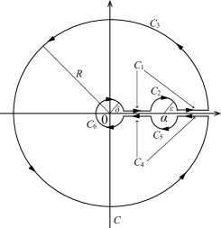
Figure 2: The contour $C$ on $\mathbb{C}$, where $\alpha\in(0,\infty)$. It consists of the paths $C_{1},\cdots,C_{6}$.

Next we give a proof of (2.30). For this purpose we first show the following relation. Let $I_{j}(x),~{}j=1,2,\cdots$, $x\in(0,\infty)$, be

$$I_{j}(x)=\int_{0}^{\infty}dw\,\frac{1}{x-w}\frac{(\log w)^{j-1}}{w+1}.$$ (A.6)

Then we have

$$I_{j}(x)=\frac{1}{x+1}\,r_{j}(\log x),$$ (A.7)

where $r_{k}(x)~{}(k=0,1,2,\cdots)$ is a $k$th order polynomial of $x$ where the coefficient of the highest degree is $1/k$. This relation (A.7) can be derived by considering the integration of $m_{j}(w;x):=(\log w)^{j}/((x-w)(w+1)),~{}x>0$ with respect to $w$ along the contour $C$ in Fig. 2 with $\alpha=x$ and $R>1$.

Note that

$$\int_{C}dw\,m_{j}(w;x)=2\pi i\,\frac{(\pi i)^{j}}{x+1},$$ (A.8)

where RHS corresponds to the residue of $m_{j}(w;x)$ at $w=-1$. As in the previous case (A.4), one easily gets

$$\lim_{\scriptstyle\delta\rightarrow 0,\epsilon\rightarrow 0\atop R\rightarrow\infty}\int_{C_{1}}dw\,m_{j}(w;x)=I_{j+1}(x),$$

$$\lim_{\scriptstyle\delta\rightarrow 0,\epsilon\rightarrow 0\atop R\rightarrow\infty}\int_{C_{4}}dw\,m_{j}(w;x)=-\int_{0}^{\infty}dw\,m_{j}(we^{2\pi i};x)=-\int_{0}^{\infty}dw\,\frac{(\log w+2\pi i)^{j}}{(x-w)(w+1)}$$

$$\hskip 122.34692pt=-\sum_{k=0}^{j}\binom{j}{k}(2\pi i)^{j-k}I_{k+1}(x),$$

$$\lim_{\epsilon\rightarrow 0}\int_{C_{2}}dw\,m_{j}(w;x)=\pi i\,\frac{(\log x)^{j}}{x+1},~{}~{}\lim_{\epsilon\rightarrow 0}\int_{C_{5}}m_{j}(w;x)dw=\pi i\,\frac{(\log x+2\pi i)^{j}}{x+1},$$

$$\lim_{R\rightarrow\infty}\int_{C_{3}}dw\,m_{j}(w;x)=\lim_{\delta\rightarrow 0}\int_{C_{6}}dw\,m_{j}(w;x)=0.$$ (A.9)

Substituting (A.9) into (A.8), we find

$$2\pi i\frac{(\pi i)^{j}}{x+1} =\lim_{\scriptstyle\delta\rightarrow 0,\epsilon\rightarrow 0\atop R\rightarrow\infty}\sum_{k=1}^{6}\int_{C_{k}}dw\,m_{j}(w;x)$$

$$=I_{j+1}(x)-\sum_{k=0}^{j}\binom{j}{k}(2\pi i)^{j-k}I_{k+1}(x)+\frac{\pi i}{x+1}\left((\log x)^{j}+\left(\log x+2\pi i\right)^{j}\right).$$ (A.10)

Thus we obtain

$$I_{j}(x)=\frac{(\log x)^{j}+(\log x+2\pi i)^{j}-2(\pi i)^{j}}{2j(x+1)}-\frac{1}{j}\sum_{k=0}^{j-2}\binom{j}{k}(2\pi i)^{j-1-k}I_{k+1}(x)$$ (A.11)

which leads to (A.7).

Here we show (2.30). We find that (2.30) is rewritten as

$$J_{B}^{*(m)}J_{F}(x)=q_{m}\left(\frac{\log x}{\beta}\right)J_{F}(x),$$ (A.12)

where $q_{m}(x)$ is defined below (2.30) and the functions $J_{F}(x)$ and $J_{B}(x)$ on $\mathbb{R}_{+}$ are defined by $J_{F}(x)=1/(x+1)$ and $J_{B}(x)=1/\beta x$.

We prove (A.12) by using (A.7) and by mathematical induction: suppose that (A.12) holds for $m=N-1$. Then we get

$$J^{*(N)}_{B}J_{F}(x) =\frac{1}{\beta}\int_{0}^{\infty}dy\,\frac{1}{x-y}J^{*(N-1)}_{B}J_{F}(y)=\frac{1}{\beta^{N}(N-1)!}I_{N}(y)+\sum_{k=0}^{N-2}\frac{c_{k}}{\beta^{k+1}}I_{k+1}(y)$$ (A.13)

where $c_{k}(k=0,1,\cdots,N-2)$ is the coefficient of $x^{k}$ in $q_{N-1}(x)$ and in the last equality we used the assumption for the mathematical induction and (A.6). Considering (A.7), we arrive at (A.12). ∎

Appendix B Proof of Lemma 10.

To show Lemma 10, we will use the following identity. For $(x_{1},\cdots,x_{N-1})\in\mathbb{R}^{N-1}$ satisfying $x_{1}>\cdots>x_{N-1}$ and $(y_{1},\cdots,y_{N})\in\mathbb{R}^{N}$, we have

$$\sum_{\sigma\in S_{N}}{\rm{sgn}}\sigma\prod_{j=2}^{N}1_{>0}\left(x_{j-1}-y_{\sigma(j)}\right)=\sum_{\sigma\in S_{N}}{\rm{sgn}}\sigma\prod_{j=2}^{N}1_{>0}\left(x_{j-1}-y_{\sigma(j)}\right)1_{>0}\left(y_{\sigma(j-1)}-x_{j-1}\right).$$ (B.1)

where $S_{N}$ is the permutation of $(1,2,\cdots,N)$. For the proof of (B.1), it is sufficient to show for $m=1,2,\cdots,N$,

$$\sum_{\sigma\in S_{N}}{\rm{sgn}}\sigma\prod_{j=2}^{N}1_{>0}(x_{j-1}-y_{\sigma(j)})\cdot\prod_{k=2}^{m}1_{>0}(y_{\sigma(k-1)}-x_{k-1})\cdot 1_{>0}(x_{m}-y_{\sigma(m)})=0,$$ (B.2)

where, as in (B.1), we assume the condition $x_{1}>x_{2}>\cdots>x_{N-1}$. This can easily be obtained by noting that

$$\sum_{\sigma\in S_{N}}{\rm{sgn}}\sigma\prod_{j=2}^{N}1_{>0}(x_{j-1}-y_{\sigma(j)})\cdot\prod_{k=2}^{m}1_{>0}(y_{\sigma(k-1)}-x_{k-1})\cdot 1_{>0}(x_{m}-y_{\sigma(m)})$$

$$=\sum_{\sigma\in S_{N}}{\rm{sgn}}\sigma\prod_{\begin{subarray}{c}j=2\\ j\neq m\end{subarray}}^{N}1_{>0}(x_{j-1}-y_{\sigma(j)})\cdot\prod_{k=2}^{m}1_{>0}(y_{\sigma(k-1)}-x_{k-1})\cdot 1_{>0}(x_{m}-y_{\sigma(m)})$$

$$=\sum_{\sigma\in S_{N}}{\rm{sgn}}\sigma\prod_{\begin{subarray}{c}j=2\\ j\neq m,~{}m+1\end{subarray}}^{N}1_{>0}(x_{j-1}-y_{\sigma(j)})\cdot\prod_{k=2}^{m}1_{>0}(y_{\sigma(k-1)}-x_{k-1})\cdot 1_{>0}(x_{m}-y_{\sigma(m)})1_{>0}(x_{m}-y_{\sigma(m+1)})$$

$$=0$$ (B.3)

where in the first equality we used the fact that the factor $1_{>0}(x_{m-1}-y_{\sigma(m)})$ can be omitted in this equation thanks to the factor $1_{>0}(x_{m}-y_{\sigma(m)})$ with the condition $x_{m-1}>x_{m}$ and the last equality follows from the fact that the term with $\sigma$ cancels the term with $\sigma^{\prime}$ where $\sigma^{\prime}$ is defined in terms of $\sigma$ as $\sigma^{\prime}(m)=\sigma(m+1)$ and $\sigma^{\prime}(m+1)=\sigma(m)$ with $\sigma^{\prime}(k)=\sigma(k)$ for $k\neq m,~{}m+1$.

Using (B.2), we have for $x_{1}>x_{2}>\cdots>x_{N-1}$

$$\sum_{\sigma\in S_{N}}{\rm{sgn}}\sigma\prod_{j=2}^{N}1_{>0}\left(x_{j-1}-y_{\sigma(j)}\right)=\sum_{\sigma\in S_{N}}{\rm{sgn}}\sigma\prod_{j=2}^{N}1_{>0}\left(x_{j-1}-y_{\sigma(j)}\right)\cdot(1-1_{>0}(x_{1}-y_{\sigma(1)}))$$

$$=\sum_{\sigma\in S_{N}}{\rm{sgn}}\sigma\prod_{j=2}^{N}1_{>0}\left(x_{j-1}-y_{\sigma(j)}\right)\cdot 1_{>0}(y_{\sigma(1)}-x_{1})$$

$$=\sum_{\sigma\in S_{N}}{\rm{sgn}}\sigma\prod_{j=2}^{N}1_{>0}\left(x_{j-1}-y_{\sigma(j)}\right)\cdot 1_{>0}(y_{\sigma(1)}-x_{1})(1-1_{>0}(x_{2}-y_{\sigma(2)}))$$

$$=\sum_{\sigma\in S_{N}}{\rm{sgn}}\sigma\prod_{j=2}^{N}1_{>0}\left(x_{j-1}-y_{\sigma(j)}\right)\cdot\prod_{k=1}^{2}1_{>0}(y_{\sigma(k)}-x_{k}).$$ (B.4)

where for the first and the third equality, we used (B.2) with $m=1$ and $m=2$ respectively. Performing the procedure in (B.4) repeatedly, we arrive at (B.1).

Now we give a proof of the lemma by the mathematical induction. The case $N=1$ in is trivial. Suppose that it holds for $N-1$. Then noticing

$$1_{V_{N}}(\underline{x}_{N})=\prod_{k=2}^{N}\prod_{j=2}^{k}1_{>0}\left(x^{(k-1)}_{j-1}-x^{(k)}_{j}\right)=1_{V_{N-1}}(\underline{x}_{N-1})\prod_{j=2}^{N}1_{>0}\left(x^{(N-1)}_{j-1}-x^{(N)}_{j}\right),$$ (B.5)

we see that LHS of (3.41) is written as

$$~{}\sum_{\sigma^{(j)}\in S_{j},j=1,\cdots,N}{\rm{sgn}}\sigma^{(N)}\,1_{V_{N-1}}(\underline{x}_{N-1}^{\sigma})\prod_{j=2}^{N}1_{>0}\left(x^{(N-1)}_{\sigma^{(N-1)}(j-1)}-x^{(N)}_{\sigma^{(N)}(j)}\right)$$

$$=\sum_{\sigma^{(j)}\in S_{j},j=1,\cdots,N}{\rm{sgn}}\sigma^{(N-1)}\,1_{V_{N-1}}(\underline{x}_{N-1}^{\sigma})\cdot{\rm{sgn}}\sigma^{(N)}\prod_{j=2}^{N}1_{>0}\left(x^{(N-1)}_{j-1}-x^{(N)}_{\sigma^{(N)}(j)}\right)$$

$$=\sum_{\sigma^{(j)}\in S_{j},j=1,\cdots,N}{\rm{sgn}}\sigma^{(N-1)}\,1_{\text{GT}}(\underline{x}_{N-1}^{\sigma})\cdot{\rm{sgn}}\sigma^{(N)}\prod_{j=2}^{N}1_{>0}\left(x^{(N-1)}_{j-1}-x^{(N)}_{\sigma^{(N)}(j)}\right)$$

$$=\sum_{\sigma^{(j)}\in S_{j},j=1,\cdots,N}{\rm{sgn}}\sigma^{(N)}\,1_{\text{GT}}(\underline{x}_{N-1}^{\sigma})\prod_{j=2}^{N}1_{>0}\left(x^{(N-1)}_{\sigma^{(N-1)}(j-1)}-x^{(N)}_{\sigma^{(N)}(j)}\right),$$ (B.6)

where in the second equality we used the assumption for $N-1$. Note that in the rightmost side of (B.6), the condition $x^{(N-1)}_{\sigma^{(N-1)}(1)}>x^{(N-1)}_{\sigma^{(N-1)}(2)}>\cdots>x^{(N-1)}_{\sigma^{(N-1)}(N-1)}$ holds for the support of $1_{\text{GT}}(\underline{x}_{N-1}^{\sigma})$. Thus we can apply (B.1) to the rightmost side. We see that it becomes

$$~{}\sum_{\sigma^{(j)}\in S_{j},j=1,\cdots,N}{\rm{sgn}}\sigma^{(N)}\,1_{\text{GT}}(\underline{x}_{N-1}^{\sigma})\prod_{j=2}^{N}1_{>0}\left(x^{(N-1)}_{\sigma^{(N-1)}(j-1)}-x^{(N)}_{\sigma^{(N)}(j)}\right)1_{>0}\left(x^{(N)}_{\sigma^{(N)}(j-1)}-x^{(N-1)}_{\sigma^{(N-1)}(j-1)}\right)$$

$$=\sum_{\sigma^{(j)}\in S_{j},j=1,\cdots,N}{\rm{sgn}}\sigma^{(N)}\,1_{\rm{GT}}(\underline{x}_{N}^{\sigma}),$$ (B.7)

which completes the proof of Lemma 10.

∎

Appendix C The saddle point analysis of $\psi_{k}(x;t)$

In this Appendix, we give a proof of (5.42) based on the saddle point method in a similar way to Sec. 5.4.3 in [10]. Here we deal with the case of general $Y$ while the case of $Y=0$ was considered in [10]. We focus mainly on the limit about $\psi_{k}(x;t)$ (2.1) in (5.42) since the case $\phi_{k}(x;t)$ (4.1) can also be estimated in a parallel way. Changing the variable as $w=-i\sqrt{N}z$, (2.1) becomes

$$\psi_{k}(x,t)=\frac{\sqrt{N}}{2\pi i}\int_{-i\infty}^{i\infty}dz\,e^{f_{N}(z;t,x)},$$ (C.1)

where

$$f_{N}(z;t,x)=-\sqrt{N}zx+N\frac{z^{2}t}{2}+(k-N)\log(\sqrt{N}z)-N\log\Gamma(\sqrt{N}z).$$ (C.2)

Substituting (5.41) and (5.43) into (C.2), we arrange the first three terms in ascending order of powers of $N$ as

$$~{}-\sqrt{N}zx_{i}+N\frac{z^{2}t}{2}+(k-N)\log(\sqrt{N}z)$$

$$=N^{3/2}\log N\cdot\frac{z}{2}+N^{3/2}\left(-z+\frac{T^{1/2}z^{2}}{2}-\frac{z}{2}\log T\right)+N\left(\gamma_{T}^{2}Yz^{2}-2\gamma_{T}^{2}YT^{-1/2}z-\frac{T^{1/2}z}{2}\right)$$

$$~{}~{}+N^{1/2}\log N\cdot\frac{\lambda}{2(2\gamma_{T})^{1/2}}+N^{1/2}\left(\frac{\gamma_{T}^{3}}{12}z-\gamma_{T}\xi_{i}z+\gamma_{T}Y^{2}z-\gamma_{T}^{2}Yz+\frac{\lambda}{(2\gamma_{T})^{1/2}}\log z\right).$$ (C.3)

Using the Stirling formula

$$\log\Gamma(n)=n\log n-n-\frac{\log 2\pi n}{2}+\frac{1}{12n}+O(n^{-3})$$ (C.4)

for the last term in (C.2), we have

$$-N\log\Gamma(\sqrt{N}z) =-N^{3/2}\log N\cdot\frac{z}{2}+N^{3/2}\left(z-z\log z\right)+\frac{N}{4}\log N+N\frac{\log 2\pi z}{2}$$

$$~{}~{}~{}~{}-N^{1/2}\frac{1}{12z}+O(N^{-1/2}).$$ (C.5)

Thus from (C.3) and (C.5), $f_{N}(z)$ (C.2) can be expressed as

$$f_{N}(z;t,x)=N^{3/2}f(z)+Ng(z)+N^{1/2}h(z)+C_{1}+O(N^{-1/2}),$$ (C.6)

$$f(z)=\frac{T^{1/2}z^{2}}{2}-z\log z-\frac{z}{2}\log T,$$ (C.7)

$$g(z)=-\frac{T^{1/2}z}{2}+\frac{\log z}{2}+\gamma_{T}^{2}Yz^{2}-\frac{2\gamma_{T}^{2}Y}{T^{1/2}}z,$$ (C.8)

$$h(z)=-\frac{1}{12z}+\left(\frac{\gamma_{T}^{3}}{12}-\gamma_{T}^{2}Y-\gamma_{T}(\xi_{i}-Y^{2})\right)z+\frac{\lambda}{(2\gamma_{T})^{1/2}}\log z.$$ (C.9)

Here $C_{1}$, which does not depend on $z$ is written as

$$C_{1}=N^{1/2}\log N\cdot\frac{\lambda}{2(2\gamma_{T})^{1/2}}+\frac{N}{2}\log 2\pi\sqrt{N}.$$ (C.10)

We note that $f(z)$ above has a double saddle point $z_{c}=T^{-1/2}$ such that $f^{\prime}(z_{c})=f^{\prime\prime}(z_{c})=0$. We expand $f(z),~{}g(z),~{}h(z)$ around $z_{c}$. Noting $f^{\prime\prime\prime}(z_{c})=2\gamma_{T}^{3}$, $g^{\prime}(z_{c})=0,~{}g^{\prime\prime}(z_{c})=2\gamma_{T}^{2}Y-\gamma_{T}^{3}$, $h^{\prime}(z_{c})=\gamma_{T}^{3}/4-\gamma_{T}^{2}Y+\gamma_{T}(\lambda-\xi_{i}+Y^{2})$, we get

$$N^{3/2}f(z) =N^{3/2}f(z_{c})+\frac{N^{3/2}}{3!}f^{\prime\prime\prime}(z_{c})(z-z_{3})^{3}+O(N^{3/2}(z-z_{c})^{4})$$

$$=C_{2}+N^{3/2}\frac{\gamma_{T}^{3}}{3}(z-z_{c})^{3}+O(N^{3/2}(z-z_{c})^{4}),$$ (C.11)

$$Ng(z) =Ng(z_{c})+Ng^{\prime}(z_{c})(z-z_{c})+N\frac{g^{\prime\prime}(z_{c})}{2}(z-z_{c})^{2}+O(N(z-z_{c})^{3})$$

$$=C_{3}-N\left(\frac{\gamma_{T}^{3}}{2}-\gamma_{T}^{2}Y\right)(z-z_{c})^{2}+O(N(z-z_{c})^{3}),$$ (C.12)

$$N^{1/2}h(z) =N^{1/2}h(z_{c})+N^{1/2}h^{\prime}(z_{c})(z-z_{c})+C_{4}+O(N^{1/2}(z-z_{c})^{2})$$

$$=C_{4}+N^{1/2}\left(\frac{\gamma_{T}^{3}}{4}-\gamma_{T}^{2}Y+\gamma_{T}(\lambda-\xi+Y^{2})\right)(z-z_{c})+O(N^{1/2}(z-z_{c})^{2}),$$ (C.13)

where $C_{2},~{}C_{3}$ and $C_{4}$ are

$$C_{2}:=N^{3/2}f(z_{c})=N^{3/2}T^{-1/2}/2,~{}~{}C_{3}:=Ng(z_{c})=-N\left(\frac{1+\log T}{2}+\frac{Y}{2\gamma_{T}}\right),$$

$$C_{4}:=N^{1/2}h(z_{c})=-N^{1/2}\left(\frac{T^{1/2}}{24}+(\gamma_{T}^{2}Y+\gamma_{T}(\xi-Y^{2}))T^{-1/2}-\frac{\lambda\log T^{-1/2}}{(2\gamma_{T})^{1/2}}\right).$$ (C.14)

Thus from (C.6)–(C.13) and under the scaling $\frac{z^{\prime}}{\sqrt{N}}=(z-z_{c})$, we have

$$f_{N}(z;t,x_{i})=\frac{\gamma_{T}^{3}}{3}\left(z^{\prime}+\frac{Y}{\gamma_{T}}-\frac{1}{2}\right)^{3}-\gamma_{T}(\xi-\lambda)\left(z^{\prime}+\frac{Y}{\gamma_{T}}-\frac{1}{2}\right)+\sum_{j=1}^{5}C_{j}+O\left(N^{-1/2}\right),$$ (C.15)

where $C_{1},\cdots,C_{4}$ are defined in (C.10) and (C.14) and $C_{5}$ is

$$C_{5}=-\frac{1}{3}\left(Y-\frac{\gamma_{T}}{2}\right)^{3}+\left(\xi-\lambda\right)\left(Y-\frac{\gamma_{T}}{2}\right).$$ (C.16)

Further changing the variable $z^{\prime}+Y/\gamma_{T}-1/2=-iv/\gamma_{T}$, we obtain

$$f_{N}(z;t,x_{i})=\frac{i}{3}v^{3}+i(\xi_{i}-\lambda)v+\sum_{j=1}^{5}C_{j}+O\left(N^{-1/2}\right),$$ (C.17)

Hence from (C.1) and (C.17), we get the limiting form of $\psi_{k}(x_{i};t)$

$$e^{-\sum_{j=1}^{5}C_{j}}\gamma_{T}\psi_{k}(x_{i};t)\sim\frac{1}{2\pi}\int_{-\infty}^{\infty}dv\,e^{\frac{i}{3}v^{3}+i(\xi_{i}-\lambda)v}={\rm Ai}(\xi_{i}-\lambda),$$ (C.18)

which is nothing but (5.42).

As with (C.1), we rewrite $\phi_{k}(x;t)$ (4.1) by the change of variable $v=\sqrt{N}z$,

$$\phi_{k}(x;t)=\frac{1}{2\pi i}\oint dz\,\frac{e^{-f_{N}(z;t,x)}}{z},$$ (C.19)

where $f_{N}(z;t,x)$ is given in (C.2). Applying the same techniques as above to this equation, we get the result for $\phi_{k}(x;t)$.

References

- [1] T. Alberts, K. Khanin, and J. Quastel, The intermediate disorder regime for directed polymers in dimension 1+1, Ann. Probab. 42 (2014), 1212–1256.
- [2] G. Amir, I. Corwin, and J. Quastel, Probability distribution of the free energy of the continuum directed random polymer in 1 + 1 dimensions, Comm. Pure. Appl. Math. 64 (2011), 466–537.
- [3] G. W. Anderson, A. Guionnet, and O. Zeitouni, An Introduction to Random Matrices, Cambridge, 2010.
- [4] C. Andréief, Note sur une relation les integrales de nies des produits des fonctions, Mém. de la Soc. Sci. Bordeaux 2 (1883), 1–14.
- [5] G. E. Andrews, R. Askey, and R. Roy, Special Functions, Cambridge, 2014.
- [6] G. Barraquand and I. Corwin, Random-walk in Beta-distributed random environment, (2015), arXiv:1503.04117.
- [7] Yu. Baryshnikov, GUEs and queues, Probab. Theory Related Fields 119 (2001), 256–274.
- [8] L. Bertini and N. Cancrini, The stochastic heat equation: Feynman-Kac formula and intermittence, J. Stat. Phys. 78 (1995), 1377–1401.
- [9] L. Bertini and G. Giacomin, Stochastic Burgers and KPZ equations from particle systems, Commun. Math. Phys. 183 (1997), 571–607.
- [10] A. Borodin and I. Corwin, Macdonald processes, Probab. Theory Related Fields 158 (2014), 225–400.
- [11] A. Borodin, I. Corwin, and P. L. Ferrari, Free Energy Fluctuations for Directed Polymers in Random Media in 11Dimension, Comm. Pure Appl. Math. 67 (2014), 1129–1214.
- [12] A. Borodin, I. Corwin, P. L. Ferrari, and B. Vető, Height Fluctuations for the Stationary KPZ Equation , Math. Phys. Anal. Geom. 18 (2015), 20 (95pages).
- [13] A. Borodin, I. Corwin, and D. Remenik, Log-Gamma Polymer Free Energy Fluctuations via a Fredholm Determinant Identity, Commun. Math. Phys. 324 (2013), 215–232.
- [14] A. Borodin, I. Corwin, and T. Sasamoto, From duality to determinants for q-TASEP and ASEP, Ann. Probab. 42 (2014), 2314–2382.
- [15] A. Borodin and P. L. Ferrari, Large time asymptotics of growth models on space-like paths I: PushASEP, Electron. J. Probab. 13 (2008), 1380–1418.
- [16] , Anisotropic Growth of Random Surfaces in Dimensions, Commun. Math. Phys. 325 (2014), 603–684.
- [17] A. Borodin, P. L. Ferrari, and M. Prähofer, Fluctuations in the discrete TASEP with periodic initial configurations and the Airy1 process, Int. Math. Res. Papers 2007 (2007), rpm002.
- [18] A. Borodin, P. L. Ferrari, M. Prähofer, and T. Sasamoto, Fluctuation properties of the TASEP with periodic initial configuration, J. Stat. Phys. 129 (2007), 1055–1080.
- [19] A. Borodin, P. L. Ferrari, and T. Sasamoto, Large time asymptotics of growth models on space-like paths II: PNG and parallel TASEP, Commun. Math. Phys. 283 (2008), 417–449.
- [20] , Transition between Airy1 and Airy2 processes and TASEP fluctuations, Commun. Pure Appl. Math. 61 (2008), 1603–1629.
- [21] , Two Speed TASEP, J. Stat. Phys. 137 (2009), 936–977.
- [22] D. Bump, The Rankin Selberg method: A survay, Number Theory, Trace Formulas and Discrete Groups (1989), 49–109, Academic Press, New York.
- [23] P. Calabrese and P. Le Doussal, Exact solution for the KPZ equation with flat initial conditions , Phys. Rev. Lett. 106 (2011), 250603.
- [24] P. Calabrese, P. Le Doussal, and A. Rosso, Free-energy distribution of the directed polymer at high temperature, EPL 90 (2010), 20002.
- [25] I. Corwin, N. O’Connell, T. Seppäläinen, and N. Zygouras, Tropical Combinatorics and Whittaker Functions, Duke Math. J. 163 (2014), 513–563.
- [26] I. Corwin, T. Seppäläinen, and H. Shen, The Strict-Weak Lattice Polymer, J. Stat. Phys. 160 (2015), 1027–1053.
- [27] I. Corwin and L-C. Tsai, KPZ equation limit of higher-spin exclusion processes, (2015), arXiv:1505.04158.
- [28] D. S. Dean, P. Le Doussal, S. N. Majumdar, and G. Schehr, Finite temperature free fermions and the Kardar-Parisi-Zhang equation at finite time, Phys. Rev. Lett. 114 (2015), 110402.
- [29] V. Dotsenko, Bethe ansatz derivation of the Tracy-Widom distribution for one-dimensional directed polymers, EPL 90 (2010), 20003.
- [30] , Replica Bethe ansatz derivation of the Tracy-Widom distribution of the free energy fluctuations in one-dimensional directed polymers, J. Stat. Mech. (2010), P07010.
- [31] F. J. Dyson, A Brownian-Motion Model for the Eigenvalues of a Random Matrix, J. Math. Phys. 3 (1962), 1191–1198.
- [32] P. L. Ferrari, H. Spohn, and T. Weiss, Brownian Motions with One-Sided Collisions: The Stationary Case, (2015), arXiv:1502.01468.
- [33] , Scaling limit for Brownian motions with one-sided collisions, Ann. Appl. Probab. 25 (2015), 1349–1382.
- [34] P. L. Ferrari and B. Vető, Tracy-Widom asymptotics for q-TASEP, Ann. Inst. H. Poincaré Probab. Statist. 51 (2015), 1465–1485.
- [35] P. J. Forrester, Log-Gases and Random Matrices, Princeton, 2010.
- [36] J. Gravner, C. A. Tracy, and H. Widom, Limit theorems for height fluctuations in a class of discrete space and time growth models, J. Stat. Phys. 102 (2001), 1085–1132.
- [37] M. Hairer, Solving the KPZ equation, Ann. Math. 178 (2013), 559–664.
- [38] T. Imamura and T. Sasamoto, Exact Solution for the Stationary Kardar-Parisi-Zhang Equation, Phys. Rev. Lett. 108 (2012), 190603.
- [39] , Stationary Correlations for the 1D KPZ Equation, J. Stat. Phys. 150 (2013), 908–939.
- [40] K. Itô, Multiple Wiener Integral, J. Math. Soc. Jpn. 3 (1951), 157–169.
- [41] C. Janjigian, Large deviations of the free energy in the O’Connell-Yor polymer, J. Stat. Phys. 160 (2015), 1054–1080.
- [42] K. Johansson, Shape fluctuations and random matrices, Commun. Math. Phys. 209 (2000), 437–476.
- [43] , Discrete polynuclear growth and determinantal processes, Commun. Math. Phys. 242 (2004), 277–329.
- [44] M. Kardar, G. Parisi, and Y. C. Zhang, Dynamic scaling of growing interfaces, Phys. Rev. Lett. 56 (1986), 889–892.
- [45] M. Katori, O’Connell’s process as a vicious Brownian motion, Phys. Rev. E 84 (2011), 061144.
- [46] , Survival probability of mutually killing Brownian motions and the O’Connell process, J. Stat. Phys. 147 (2012), 206–223.
- [47] , System of complex Brownian motions associated with the O’Connell process, J. Stat. Phys. 149 (2012), 411–431.
- [48] A. Kupiainen, Renormalization Group and Stochastic PDEs, Ann. Henri Poincaré 17 (2016), 497–535.
- [49] P. Le Doussal and P. Calabrese, The KPZ equation with flat initial condition and the directed polymer with one free end, J. Stat. Mech. (2012), P06001.
- [50] I. G. Macdonald, Symmetric Functions and Hall Polynomials, Oxford, 1995.
- [51] P. Major, Multiple Wiener-Itô integrals with applications to limit theorems, Lecture Notes in Math. 849 (2013), 2nd edition.
- [52] M. L. Mehta, Random Matrices, Elsevier, 2004.
- [53] G. Moreno Flores and J. Quastel, unpublished.
- [54] J. Moriarty and N. O’Connell, On the free energy of a directed polymer in a Brownian environment, Markov Processes and Related Fields 13 (2007), 251–266.
- [55] C. Mueller, On the support of solutions to the heat equation with noise, Stochastics and Stochastics Reports 37 (1991), 225–245.
- [56] T. Nagao and T. Sasamoto, Asymmetric simple exclusion process and modified random matrix ensembles, Nucl. Phys. B 699 (2004), 487–502.
- [57] N. O’Connell, Directed polymers and the quantum Toda lattice, Ann. Probab. 40 (2012), 437–458.
- [58] N. O’Connell and J. Ortmann, Tracy-Widom asymptotics for a random polymer model with gamma-distributed weights, Electron. J. Probab. 20 (2015), 1–18.
- [59] N. O’Connell and M. Yor, Brownian analogues of Burke’s theorem, Stochastic Process. Appl. 96 (2001), 285–304.
- [60] A. Okounkov and N. Reshetikhin, Correlation function of Schur process with application to local geometry of a random 3-dimensional Young diagram, J. Amer. Math. Soc. 16 (2003), 581–603.
- [61] N. O’Connell, T. Seppäläinen, and N. Zygouras, Geometric RSK correspondence, Whittaker functions and symmetrized random polymers, Invent. Math. 197 (2014), 361–416.
- [62] J. Ortmann, J. Quastel, and D. Remenik, A Pfaffian representation for flat ASEP, (2015), arXiv:1501.05626.
- [63] , Exact formulas for random growth with half-flat initial data, Ann. Appl. Probab. 26 (2016), 507–548.
- [64] A. Rakos and G. M. Schütz, Current distribution and random matrix ensembles for an integrable asymmetric fragmentation process, J. Stat. Phys. 118 (2005), 511–530.
- [65] T. Sasamoto, Spatial correlations of the 1D KPZ surface on a flat substrate, J. Phys. A 38 (2005), L549–L556.
- [66] T. Sasamoto and H. Spohn, Exact height distributions for the KPZ equation with narrow wedge initial condition, Nuc. Phys. B 834 (2010), 523–542.
- [67] , One-Dimensional Kardar-Parisi-Zhang Equation: An Exact Solution and its Universality, Phys. Rev. Lett. 104 (2010), 230602.
- [68] , The -dimensional Kardar-Parisi-Zhang equation and its universality class, J. Stat. Mech. (2010), P11013.
- [69] , The Crossover regime for the weakly asymmetric simple exclusion process, J. Stat. Phys. 140 (2010), 209–231.
- [70] T. Sasamoto and M. Wadati, Determinant form solution for the derivative nonlinear Schrödinger type model, J. Phys. Soc. Jpn. 67 (1998), 784–790.
- [71] G. M. Schütz, Exact solution of the master equation for the asymmetric exclusion process, J. Stat. Phys. 88 (1997), 427–445.
- [72] T. Seppäläinen and B. Valkó, Bounds for scaling exponents for a 1+1 dimensional directed polymer in a Brownian environment, ALEA 7 (2010), 451–476.
- [73] A. Soshnikov, Determinantal random point fields, Russian Math. Surveys 55 (2000), 923–975.
- [74] E. Stade, Archimedean -factors on GLGL(n) and generalized Barnes integrals, Israel J. Math. 127 (2002), 201–219.
- [75] C. A. Tracy and H. Widom, Level-spacing distributions and the Airy kernel, Commun. Math. Phys. 159 (1994), 151–174.
- [76] , Correlation functions, cluster functions, and spacing distributions for random matrices, J. Stat. Phys. 92 (1998), 809–835.
- [77] B. Vető, Tracy-Widom limit of q-Hahn TASEP, Electron. J. Probab. 20 (2015), 1–22.
- [78] J. Warren, Dyson’s Brownian motions, intertwining and interlacing, Electron. J. Probab. 12 (2007), 573–590.