Analyzing TCP Throughput Stability and Predictability with Implications for Adaptive Video Streaming

Abstract

Recent work suggests that TCP throughput stability and predictability within a video viewing session can inform the design of better video bitrate adaptation algorithms. Despite a rich tradition of Internet measurement, however, our understanding of throughput stability and predictability is quite limited. To bridge this gap, we present a measurement study of throughput stability using a large-scale dataset from a video service provider. Drawing on this analysis, we propose a simple-but-effective prediction mechanism based on a hidden Markov model and demonstrate that it outperforms other approaches. We also show the practical implications in improving the user experience of adaptive video streaming.

1 Introduction

In recent years, we have seen a dramatic rise in the volume of HTTP-based adaptive video streaming traffic in the Internet [1]. In contrast to traditional metrics such as transfer completion time for web requests, delivering good application-level experience for video introduces new metrics such as low buffering or smooth bitrate delivery [10].

To meet these new application-level quality of experience goals, video players use dynamic bitrate adaptation within a viewing session [13, 16]. Here, the video is chunked into discrete segments, and each chunk is encoded at different bitrate levels, to enable the player to dynamically change the bitrate chosen for future video chunks in response to the operating conditions [13, 16]. Note that in this setting, delivering good application performance depends on the “consistency” of TCP throughput behavior within the session between the client and the video server, rather than the burst or average properties of the Internet path.

In this respect, understanding intra-session TCP throughput characteristics can improve our understanding of existing video adaptation strategies (e.g., [23]) and inform the development of new algorithms (e.g., [23, 25]). Specifically, there are two key questions that we wish to address:

• Stability: If the TCP throughput is stable, then adaptive video streaming algorithms can avoid frequent switches and pick the highest possible bitrate that does not induce buffering [23, 16, 14].

• Predictability: Many adaptation algorithms use the estimated TCP throughput from previous chunks to choose the bitrates for the next few chunks. Recent work has shown that an accurate throughput predictor, if available, can significantly improve the quality of experience for adaptive video streaming [23, 25].

Despite the rich measurement literature in characterizing various Internet path properties (e.g., [15, 21, 9, 12]), our understanding of TCP throughput stability and predictability is quite limited. There has been surprisingly little work in this space and the closest related works we are aware of are dated and limited in scope [24, 7].

Our goal in this paper is to bridge this gap. To this end, this paper makes three key contributions:

• Measurement (

  2 LABEL:

  sec:analysis): We analyze the TCP throughput stability on a dataset consisting of minute-level throughput measurements from over 200K sessions from a large video provider. Our key findings are: a) A large number of sessions have significant intra-session throughput variations; b) High throughput sessions tend to be more stable; and c) The throughput is more similar in neighboring/recent time slots and less similar to measurements made further apart.

• Prediction algorithm (

  3 LABEL:

  sec:premodel): Building on observed temporal structure, we develop a simple-yet-effective algorithm based on the insight that the throughput can be modeled as a function of a hidden state variable – the number of concurrent flows at a bottleneck link. We develop a hidden Markov model (HMM) predictor and show that it outperforms a range of timeseries modeling techniques.

• Application implications (

  4 LABEL:

  sec:eval): Using trace-driven simulations, we show that our HMM predictor significantly improves the video QoE over prior work that does not use throughput predictions [13] and is very close to the optimal achievable QoE which is based on the perfect knowledge of future throughput.

5 Related work

In this section, we place our work in the context of past work in Internet measurement and adaptive video streaming.

Measuring path properties:  Prior work has measured stability of path properties such as the persistence and prevalence of routes over time [19]. Other work focuses on inter-domain routing stability and reports that popular destinations have stable routes [20]. In contrast our focus is on throughput stability and predictability.

Bandwidth measurement tools:  There are many tools for measuring the available bandwidth and the capacity of Internet paths (e.g., [4, 12]). At a high-level, they extend packet pair techniques and provide mechanisms to deal with background traffic interference. We refer readers to the survey by Jain and Dovrolis for more in-depth comparisons [15]. However, these are active probes that result in a single data point. In contrast, we use passive measurements to develop a systematic understanding of the temporal stability and predictability of the TCP throughput.

Throughput stability:  Balakrishnan et al., use throughput measurements from a large web service and report that the throughput for the same client-server pair does not change significantly (less than factor of 2) for tens of minutes [7]. Zhang et al., analyze the stability in terms of statistical, operational, and predictive metrics [24]. They report that using recent history on the scale of minutes is useful but in the order of hours misleads estimators. Unfortunately, these are dated and limited in terms of scale and scope.

Throughput prediction:  Prior work developed approximate analytical models of TCP throughput as a function of packet loss and delay [18, 11, 17]. However, these do not directly translate into actual prediction algorithms that can feed into video adaptation algorithms.

Broadband measurements:  Given the recent debate on network neutrality and video, measurements of broadband characteristics have regained prominence [21, 2]. However, these do not focus on throughput stability and predictability.

Adaptive video streaming over HTTP:  Our work is motivated by Dynamic Adaptive Streaming over HTTP (DASH). Prior work implicitly assumes throughput is unstable and unpredictable and eschews this in favor of using the player buffer occupancy for controlling bitrates [13]. Recent work  [23, 25] argues that adaptive video streaming can significantly benefit from accurate throughput prediction. However, these do not provide a concrete prediction algorithm. Our contribution is in developing an effective throughput predictor and demonstrating its utility for DASH.

6 Dataset

In this section, we describe the dataset we use for analyzing TCP throughput stability and predictability.

Note that in contrast to other throughput and path measurements, we need continuous measurements over sufficiently long durations (e.g., several minutes). We are not aware of public datasets that enable such in-depth analysis of throughput stability and predictability at scale. We explored datasets such as Glasnost [9], FCC [2], and from a EU cellular provider [3]. Unfortunately, all of these had too few hosts and the sessions lasted only a handful of seconds making it unusable for the stability and predictability analysis of interest for adaptive video streaming.

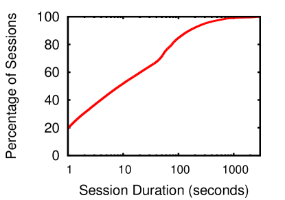
(a) Duration

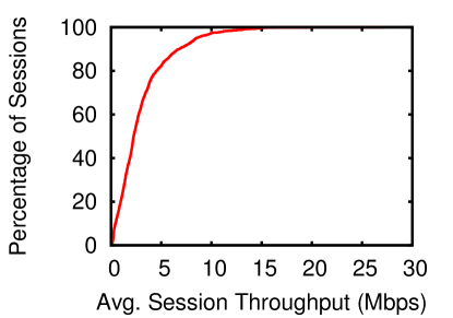
(b) Throughput

Figure 1: CDF of session duration and throughput.

Our dataset is collected from the operational CDN platform of PPTV [5]. PPTV is a leading online video content provider in China with more than 227 million users. We use measurements from real video sessions from this provider. These sessions cover $428,000$ unique client IPs and over 1000 unique server IPs. The clients span 508 cities and 28 ISPs in China. In total, we collect data from over 2.7 million sessions over a 4 day period.

Each session consists of several video “chunks”. The session is divided into 1-minute epochs, and the client reports the average TCP throughput observed within this epoch during the active download times. If there are multiple chunks transmitted in the same epoch, the throughput reported for this epoch should be the byte-weighted mean of the average throughput of each chunk. Conversely, if a chunk spans multiple epochs it contributes partially to each epoch it spans.

As observed in other studies, the duration of each session is variable [6]. Figure 1a shows the CDF of the session duration in our dataset. Since we are interested in temporal stability and predictability, we focus on sessions that last more than 6 minutes. About 10% of the sessions last more than 6 minutes still yielding a substantial number of sessions ($\geq$ 200K) for our analysis. Figure 1b shows the CDF of the per-epoch average throughput and suggests that the average throughput distribution is similar to residential broadband characteristics [21]. While this is indeed a single dataset from the Chinese Internet, based on these observations and our experience with other datasets of a similar nature (e.g., [10]) we believe that this is representative of video workloads measured in residential broadband settings.

We do acknowledge one limitation—the finest time resolution we have is 1 minute. However, we believe that understanding stability/predictability at a minute timescale is still valuable for adaptive video streaming applications and as we will show in

7 LABEL:

sec:eval it can still yield significant improvements for quality of experience.

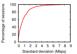
(a) Absolute stddev

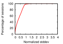
(b) Coefficient of variability

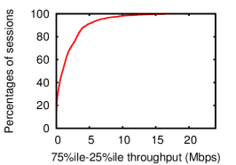
(c) Diff. between 75-th and 25-th percentile

Figure 2: Analyzing throughput stability through different metrics.

8 Intra-session throughput analysis

In this section, we analyze three key characteristics of the throughput within a client-server session:

• How variable is the throughput within a session?
  For instance, if the variability is small, then the adaptation logic does not have to switch bitrates often.

• Is the variability correlated/anti-correlated vs.  average throughput?
  If the variability is a function of the average throughput, then we may need to customize the adaptation logic for different deployments; e.g., wireless clients vs.  fiber-to-home links.

• Are there temporal patterns within the session; e.g., how similar are recent observations made $k$ minutes apart?
  This temporal structure has key implications for predictability as many adaptation algorithms use estimates of throughput over the next few chunks as part of their decision logic [23].

Intra-session variability:  First, we compute the standard deviation (“stddev”) of TCP throughput across different measurements within the session. Figure 2a shows the CDF (across sessions) of the per-session throughput stddev. We see that about 20% of sessions have a stddev $\geq$2Mbps. Second, we compute the coefficient of variation, which is the ratio of stddev to the mean. Figure 2b shows the CDF of this normalized metric; we see that the roughly 40% of sessions have normalized stddev $\geq$50%. Now, the stddev could still be biased by a few outliers even if the throughput is mostly stable. Thus, we also compute the difference between the 75-th and 25-th percentile throughput values within a session and plot the CDF in Figure 2c. Again, we see that a non-trivial fraction of sessions ($\geq$ 30%) has a difference of $>$2Mbps/s. In short, this result confirms the general perception that we need good bitrate adaptation strategies and that simple static bitrate selection will not suffice.

Variability vs. average throughput:  Next, we analyze if there is some relationship between throughput stability and the average session throughput. Based on the distribution in Figure 1b, we categorize the PPTV sessions into different 800Kbps bins. Figure 3 shows the average normalized stddev of the sessions within each bin. As a general trend, the normalized variability decreases as with increased average throughput. We posit that such high throughput sessions traverse less congested paths and thus the variability of throughput is also small. This result suggests that the throughput is more stable for higher throughput sessions and thus bitrate adaptation algorithms can afford to be less conservative compared to low throughput sessions.

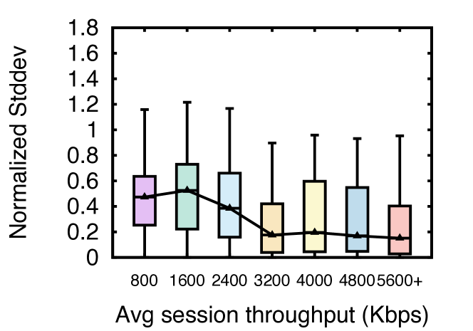
Figure 3: Normalized stddev vs. average throughput.

Temporal structure:  The above results provide an aggregate view of the variability within the session but do not shed light on the temporal structure. Such temporal structure can have key implications for predictability. For instance, consider two hypothetical sessions with the following measurements (in Mbps): (1) Session 1 = 1,1,1,0.5,0.5,0.5 and (2) Session 2 = 1,0.5,1,0.5,1,0.5. Now, both sessions have the same mean, stddev, percentile difference, but intuitively Session 1 is more predictable based on recent history than the pattern in Session 2.

To quantitatively analyze the temporal structure (i.e., how the throughput changes during the course of a session), we compute the autocorrelation of the throughput time-series for different time-shifts. Figure 4 summarizes the distribution (across sessions) of the these autocorrelations as a box-and-whiskers plot depicting the median, 25-th, 75-th percentiles and the min/max values for different time lags. While the autocorrelations are positive, we see a marked decrease as the lag increases. In other words, the throughput is more similar in recent time slots and less similar to measurements made far earlier or later.

To give some visual intuition, we show the throughput timeseries of a representative client-server session in Figure 5. Here, we see that the throughput evolves during the course of a session and thus the correlation between distant timeslots tends to be lower.

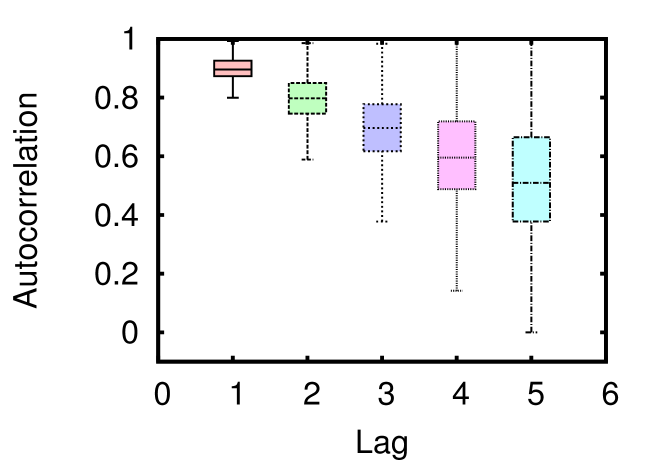
Figure 4: Autocorrelation of the throughput over different time windows (25, 50, 75%ile).

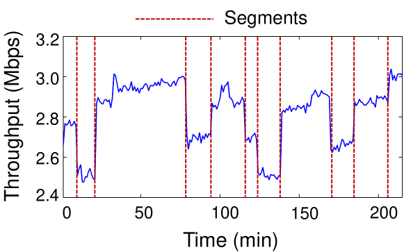
Figure 5: An example of PPTV video session throughput.

Summary of key findings::  Our throughput variability analysis shows that:

• A large number of sessions have significant variations of their intra-session throughput, with normalized stddev $\geq$50% for more than 40% of sessions.

• High throughput sessions generally are more stable than low throughput sessions.

• The throughput is more similar in recent measurements and the similarity decays with higher lag.

9 Intra-session throughput prediction

The previous section reveals significant throughput variation during a session and the need for good video bitrate adaptation schemes. Ideally, we can accurately predict the TCP throughput to select bitrates for the next few chunks to optimize user perceived quality of experience [23, 22]. However, this is challenging and the limitations of existing prediction mechanisms (

10 LABEL:

sec:premodel:strawman) have even motivated efforts that avoid throughput-based adaptation [13]. In this section, we describe a simple but effective prediction motivated by the temporal structure in the throughput. Before we do so, we describe strawman solutions considered in the literature and their limitations in light of our observations.

10.1 Strawman solutions

Our goal here is not to exhaustively enumerate all possible prediction algorithms. As such, the models we consider are representative of classical time series models used in adaptive streaming proposals [23, 11]. At a high level, a throughput prediction model can be viewed as a function of the observed throughputs over the previous $p$ epochs. Let $W_{t}$ denote the observed throughput at epoch $t$ and $\hat{W}_{t},\ldots,\hat{W}_{t+\Delta}$ denote the estimate for the next $\Delta$ epochs.

• Last Sample (LS): In the simplest case, we simply use the previous observation; i.e., $\forall i\in[t,t+\Delta]:\hat{W}_{i}=W_{t-1}$. The problem with this approach is that a single sample will be a very noisy estimator and thus may cause significant bitrate oscillations [23, 16].

• Arithmetic Mean (AM): To address the noise, we can consider “smoothing” using $p$ measurements from history; i.e., $\forall i\in[t,t+\Delta]:\hat{W}_{i}=\frac{\sum_{q=1}^{p}W_{t-q}}{p}$. However, there are still two fundamental problems. First, if we use a small $p$, outliers can still cause significant under- or overestimation. Second, if we use a large $p$, measurements made too far back in history may induce serious biases as we saw in Figure 5.

• Harmonic Mean (HM): One way to minimize the impact of outliers in AM is using a harmonic mean [16]: $\forall i\in[t,t+\Delta]:\hat{W}_{i}=\frac{1}{\sum_{q=1}^{p}\frac{1}{W_{t-q}}}$. While this addresses the outlier problem, uncorrelated measurements too far in history can still bias the predictions.

• Auto-regressive models (ARMA,AR): Auto-regressive moving average (ARMA) is a classical timeseries modeling technique [11]. The ARMA model assumes $W_{t}$ has the following form: $W_{t}=a_{0}+\sum_{j=1}^{p}a_{j}W_{t-j}+\sum_{j=1}^{q}b_{j}S_{t-j}$, where $S_{t}\sim N(0,\sigma^{2})$ is i.i.d. Gaussian noise, independent of $W_{t}$. $p,q$ are the sizes of the sliding windows for auto-regression and moving average, respectively, and $\theta_{ARMA}=\{\{a_{i}\}_{i=0}^{p},\{b_{i}\}_{i=1}^{q}\}$ are the parameters that can be learned from training data (e.g., historical sessions). The auto-regression (AR) model is a simplified version of ARMA that assumes $W_{t}=a_{0}+\sum_{j=1}^{p}a_{j}W_{t-j}+e_{t}$, where $a_{0}$ is a constant and $e_{t}$ is i.i.d. zero-mean Gaussian noise independent of $W_{t}$. $\theta_{AR}=\{\{a_{i}\}_{i=0}^{p}\}$. Given training data and $p,q$, Yule-Walker equations can be adopted to learn the parameters $\theta_{ARMA}$, or $\theta_{AR}$. The key problem with these models is that they have implicit independence and stationary assumptions. However, Figures 4 and 5 suggest that there is some inherent “stateful” and “evolving” temporal structure in the throughput, which contradicts these assumptions.

10.2 Using a Hidden Markov Model

Hidden Markov models (HMM) are widely used in many applications, ranging from speech recognition to event detection [8]. From a networking perspective, the intuition behind the use of HMM in our context is that the throughput depends on the hidden state—the number of flows sharing the bottleneck link. The visualization in Figure 5 confirms this intuition that the throughput has some stateful evolving behaviors. By capturing these state transitions and the dependency between the throughput vs. the hidden state, using HMM can yield more robust throughput predictions.

Model specification:  Suppose the throughput depends on some hidden state variables $X_{t}\in{\cal X}$, where ${\cal X}=\{x_{1},\cdots,x_{M}\}$ is the set of possible states and $M=|{\cal X}|$ is the number of states. The state evolves as a Markov process where the likelihood of the current state only depends on the last state, i.e., $\mathbb{P}(X_{t}|X_{t-1},X_{t-2},\cdots,X_{1})=\mathbb{P}(X_{t}|X_{t-1})$. We denote the transition probability matrix by $P=\{P_{ij}\}$, where $P_{ij}=\mathbb{P}(X_{t}=x_{i}|X_{t-1}=x_{j})$. We let the probability distribution vector $\pi_{t}=(\mathbb{P}(X_{t}=x_{1}),\cdots,\mathbb{P}(X_{t}=x_{M}))$. Then $\pi_{t+\tau}=\pi_{t}P^{\tau}$. Each state “emits” the throughput expected within that state. Within each hidden state $X_{t}$, we model the throughput $W_{t}$ by a Gaussian distribution; i.e., $W_{t}|X_{t}=x\ \sim N(\mu_{x},\sigma_{x}^{2})$.

To see this concretely, let us revisit Figure 5. Here, we can conceptually think of splitting the timeseries into roughly 11 segments each corresponding to a hidden state. Within each segment, the throughput is largely Gaussian; e.g., between timeslots 20–75 the throughput has mean 2900, and in slots 10-20 and 125–135 the mean is 2500.

Model learning:  Given number of states $M$, we can use training data to learn the parameters of HMM, $\theta_{HMM}=\{\pi_{0},P,\{(\mu_{x},\sigma_{x}^{2}),x\in{\cal X}\}\}$ via the expectation-maximization (EM) algorithm [8]. Note that the number of states $M$ needs to be specified. There is a tradeoff here in choosing suitable $M$. Smaller $M$ yields simpler models, but may be inadequate to represent the space of possible behaviors. On the other hand, a large $M$ leads to more complex model with more parameters, but may in turn lead to overfitting issues. We find empirically that $M=6$ is a “sweet spot” in the tradeoff (Figure 6).

Online throughput prediction:  At time $t$, given past throughput $W_{1:t-1}=\{W_{1},\cdots,W_{t-1}\}$, we first use forward-backward algorithm [8] to determine $\pi_{t-1|1:t-1}=(\mathbb{P}(X_{t-1}=x_{1}|W_{1:t-1}),\cdots,\mathbb{P}(X_{t-1}=x_{M}|W_{1:t-1}))$. Then the distribution of $X_{t+\tau}$ can be obtained by: $\pi_{t+\tau|1:t-1}=\pi_{t-1|1:t-1}P^{\tau+1}$. Finally, we compute the maximum likelihood estimate of $W_{t+\tau},\tau>0$ as $\hat{W}_{t+\tau}=\mu_{x}$, where $x=arg\max_{x\in{\cal X}}\mathbb{P}(X_{t+\tau}=x|W_{1:t-1})$.

11 Evaluation

In this section, we present trace-driven evaluations using the dataset in

12 LABEL:

sec:dataset and evaluate our proposed HMM scheme vs. strawman approaches along two dimensions: (1) Prediction accuracy and (2) Video quality of experience.

12.1 Improvement in prediction accuracy

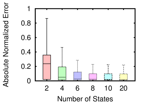
Figure 6: Error vs. HMM model size.

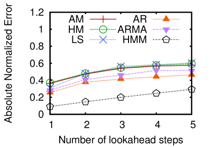
(a) 90%ile per session, and median across sessions

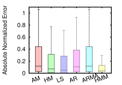
(b) Error distribution (25, 50, 75%ile)

Figure 7: Prediction accuracy of different models; LS=Last Sample, AM=ArithmeticMean, HM=Harmonic Mean, AR =AutoRegressive, ARMA = AutoRegressive Moving Average.

Setup:  To learn the various parameters (e.g., $\theta_{ARMA}$, $\theta_{HMM}$), we divide the dataset into equally-sized training and testing datasets. We learn these parameters from training dataset and report error metrics on the testing dataset. For AR model, we empirically tried different $p$ values in the training dataset and found $p=5$ yields the best result.

Error metric:  For each slot $t$ of a session $s$, we compute the absolute normalized error $\mathit{Err}_{s,t}=\frac{|\hat{W}_{s,t}-W_{s,t}|}{W_{s,t}}$, where $\hat{W}_{s,t}$ and $W_{s,t}$ denote the predicted and true throughput for slot $t$ of session $s$. Given these “atomic” error values, we can summarize the error within and across sessions in different ways; e.g., median per-session and median across sessions or median per-session and 90-th percentile across sessions.

Configuring HMM:  One natural question about the HMM is how many states $M$ we need in practice. Having more complex models with more states can decrease the error, but also increases the training time and risks of overfitting. Figure 6 shows the testing error for HMMs with varying number of states. We see that while the error decreases with more complex state models, we see a natural diminishing returns property after 6 states. As a practical tradeoff between the above considerations, we choose a 6-state HMM.

HMM vs. Strawman solutions:  Figure 7 considers two possible ways to summarize the per-slot error values. Figure 7a shows the median across sessions of the “tail” 90-percentile prediction error within a session and Figure 7b shows the overall distribution of the per-slot error values. In both cases, we see that the HMM model clearly outperforms other techniques. For instance, in Figure 7a, the HMM approach has 60% improvement over the second best predictor (AR). Similarly, in the overall distribution we see that the HMM dramatically reduces the tail of the errors; e.g., more than 75% of the predictions of HMM have less than $<$18% compared to $\geq$27% for other models. We also considered other summarizations such as median across sessions of per-session median, average-of-average etc., and found consistent results that HMM significantly outperforms the strawman models (not shown). Note that the expected benefits of HMM predictors will be even bigger when we go to finer time-scale, e.g. second-level instead of minute-level throughput prediction.

One minor downside is that the “low tail” (25 percentile) error of HMM is worse than the last-sample predictor. This is due to some highly stable sessions where throughput is constant and thus last-sample predictor has zero error. Due to the quantization effect with only 6 states, there is a small bias with HMM predictions. However, as we will see next this has no impact on the application quality of experience.

12.2 Improvement in video QoE

Next, we evaluate the improvement in user quality of experience (QoE) gained by using the improved HMM-based throughput prediction in the context of dynamic adaptive streaming over HTTP (DASH) [23, 16].

Setup:  Our goal is to evaluate the benefit of improved throughput prediction via HMM and not to evaluate the specific video adaptation heuristics or artifacts. To this end, for the adaptation algorithm we follow strategies formulated by recent efforts [23, 25], that take as input throughput predictions for the next few epochs (e.g., via harmonic mean) and solve an exact integer linear programming optimization to decide the bitrate for the next chunk. As a baseline, we also consider the buffer-based (BB) policy which does not use any throughput prediction [13].

Error metric:  Identifying suitable QoE functions for video is an open problem [6]. Here, we adopt a simple linear model suggested by previous work [23], which is the weighted sum of different factors such as average video quality, average quality variation, and total rebuffer time. We compute a normalized QoE metric of each algorithm relative to the theoretical optimal, which could be achieved with the perfect knowledge of future throughput.

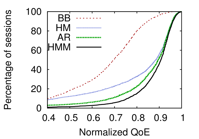
Figure 8: Adaptive video QoE improvement using throughput prediction; BB refers to the pure buffer-based adaptation that ignores throughput [13].

QoE improvement:  Figure 8 shows the CDF of the normalized QoE of different approaches. For clarity, we focus on a subset of predictors since the lines of other strawman solutions are very close to the Harmonic mean (HM) and AR. First, the result confirms observations from prior work that accurate prediction can dramatically improve QoE over the baseline buffer-based approach [23, 13]. Second, we also see the improved prediction accuracy of HMM also leads to the best QoE especially in the lower tail; e.g., the gap between the 20%ile QoE of HMM and the harmonic mean suggested in prior work [16] is almost 25%. Third, we see that the HMM-based approach is also very close to the optimal QoE achievable with perfect knowledge, with median being 90% of the optimal.

13 Conclusions

Our imminent need for understanding throughput stability and predictability is motivated by adaptive streaming over HTTP [23, 22, 25]. There is surprisingly little work on this topic and large-scale datasets on “long lived” sessions with continuous throughput measurements needed to shed light on these aspects appear to be especially scarce. Our work bridges this gap by (1) providing a large-scale measurement analysis of intra-session throughput stability and (2) an online prediction mechanism based on a hidden Markov model. We hope that our work inspires further research on this topic at more fine-grained timescales and across different deployment scenarios (e.g., cellular).

References

- [1] Cisco Visual Networking Index. http://www.cisco.com/c/en/us/solutions/service-provider/visual-networking-index-vni/index.html.
- [2] FCC Measuring Broadband America . http://www.fcc.gov/measuring-broadband-america.
- [3] HSDPA. http://home.ifi.uio.no/paalh/dataset/hsdpa-tcp-logs/.
- [4] Pathchar. http://www.caida.org/tools/utilities/others/pathchar/.
- [5] PPTV. http://www.pptv.com/.
- [6] A. Balachandran et al. A Quest for an Internet Video Quality-of-Experience Metric. In HotNets, 2012.
- [7] H. Balakrishnan et al. Analyzing Stability in WideArea Network Performance. In Proc. ACM SIGMETRICS, 1997.
- [8] C. M. Bishop. Pattern recognition and machine learning. springer, 2006.
- [9] M. Dischinger et al. Glasnost: enabling end users to detect traffic differentiation. In Proc. NSDI, 2010.
- [10] F. Dobrian et al. Understanding the impact of video quality on user engagement. In Proc. SIGCOMM, 2011.
- [11] Q. He et al. On the predictability of large transfer TCP throughput. In Proc. ACM SIGCOMM, 2005.
- [12] N. Hu et al. Locating internet bottlenecks: Algorithms, measurements, and implications. In Proc. SIGCOMM, 2004.
- [13] T. Huang et al. A Buffer-Based Approach to Rate Adaptation: Evidence from a Large Video Streaming Service. In Proc. SIGCOMM, 2014.
- [14] T.-Y. Huang et al. Confused, Timid, and Unstable: Picking a Video Streaming Rate is Hard. In Proc. IMC, 2012.
- [15] M. Jain et al. End-to-end available bandwidth: measurement methodology, dynamics, and relation with tcp throughput. IEEE/ACM Transactions on Networking, 11(4):537 – 549, 2003.
- [16] J. Jiang et al. Improving Fairness, Efficiency, and Stability in HTTP-Based Adaptive Video Streaming with Festive. IEEE/ACM Transactions on Networking, 22(1):326 – 340, 2014.
- [17] M. Mirza et al. A machine learning approach to tcp throughput prediction. In Proc. SIGMETRICS, 2007.
- [18] J. Padhye et al. Modeling TCP throughput: A Simple Model and its Empirical Validation. In Proc. SIGCOMM, 1998.
- [19] V. Paxson. End-to-End Routing Behavior in the Internet. Aug. 1996.
- [20] J. Rexford et al. BGP routing stability of popular destinations. In Proc. SIGCOMM IMC, 2002.
- [21] S. Sundaresan et al. Broadband Internet Performance: A View From the Gateway. In Proc. SIGCOMM, 2011.
- [22] G. Tian et al. Towards agile and smooth video adaptation in dynamic http streaming. In Proc. CoNEXT, 2012.
- [23] X. Yin et al. Toward a Principled Framework to Design Dynamic Adaptive Streaming Algorithms over HTTP. In Proc. HotNets, 2014.
- [24] Y. Zhang et al. On the constancy of Internet path properties. In Proc. IMW, 2001.
- [25] X. K. Zou et al. Can Accurate Predictions Improve Video Streaming in Cellular Networks? In HotMobile, 2015.