Stabilization of ring dark solitons in Bose-Einstein condensates

Abstract

Earlier work has shown that ring dark solitons in two-dimensional Bose-Einstein condensates are generically unstable. In this work, we propose a way of stabilizing the ring dark soliton via a radial Gaussian external potential. We investigate the existence and stability of the ring dark soliton upon variations of the chemical potential and also of the strength of the radial potential. Numerical results show that the ring dark soliton can be stabilized in a suitable interval of external potential strengths and chemical potentials. We also explore different proposed particle pictures considering the ring as a moving particle and find, where appropriate, results in very good qualitative and also reasonable quantitative agreement with the numerical findings.

I Introduction

Over the past few years, there has been an intense research interest, not only theoretically, but also experimentally, in the physics of atomic Bose-Einstein condensates (BECs) book1 ; book2 , and particularly in the study of nonlinear waves emergent . Bright expb1 ; expb2 ; expb3 , dark djf and gap gap matter-wave solitons, as well as vortices emergent ; fetter1 ; fetter2 , solitonic vortices and vortex rings komineas_rev are only some among the many structures studied (including more exotic ones such as Skyrmions bigelow or Dirac monopoles david ).

One of the most prototypical excitations that have been intensely studied in experiments are dark solitons djf . While the early experiments in this theme were significantly limited by dynamical instabilities and thermal effects han1 ; nist ; dutton ; han2 ; nsbec , more recent efforts have been significantly more successful in generating and exploring these structures. By now, the substantial control of the generation, and dynamical interactions of such structures has led to a wide range of experimental works monitoring their evolution in different settings engels ; Becker:Nature:2008 ; hambcol ; kip ; andreas ; jeffs .

The instability of dark solitons in higher dimensions (towards bending nist and eventual snaking towards vortices/vortex rings nsbec ; beckerus ) has been one of the key reasons for the inability to study such states in higher dimensions. Although external stabilization mechanisms, e.g., utilizing a blue-detuned laser beam manjun , have been proposed, importantly also variants of such dark solitons have been explored in higher dimensions in the form of ring dark solitons (RDSs). These efforts were at least in part motivated by works in nonlinear optics, where they initially were introduced in Ref. KYR , and studied in detail, both theoretically (in conservative thring ; djfbam ; ektoras and —more recently— in dissipative dum settings) and experimentally expring1 . In turn, RDSs in BECs were originally proposed in Ref. rds2003 and their dynamics was analyzed by means of the perturbation theory of dark matter-wave solitons djf . In other works, RDSs were studied by different approaches, e.g., in a radial box ldc1 , by using a quasi-particle approach kamch , or by considering them as exact solutions in certain versions of the Gross-Pitaevskii equation (GPE) toik1 . Proposals for the creation of RDS, e.g., by means of BEC self-interference ch1 or by employing the phase-imprinting method song , as well as generalizations of such radial states (including multi-nodal ones) ldc1 ; herring have also been considered. Moreover, generalizations of RDSs were studied in multi-component settings, in the form of dark-bright ring solitons stockhofe (emulating the intensely studied context of multi-component one-dimensional (1D) dark-bright solitons buschanglin ; sengdb ; peter1 ; peterprl ), or in the form of vector RDS in spinor $F=1$ BECs song . Importantly, structures of the form of radially symmetric dark solitons, closely connected to RDSs exist also in three-dimensions with a spherical rather than cylindrical symmetry (so-called “spherical shell solitons” ldc1 ).

Nevertheless, in none of these contexts (either one- or multi-component), was it possible to achieve complete stabilization of the RDSs. In particular, stabilization mechanisms that have been proposed, e.g., by “filling” the RDS by a bright soliton component stockhofe or by employing the nonlinearity, management (alias “Feshbach resonance management” FRM ) technique ch2 , were only able to prolong the RDSs’ life time. In fact, it was illustrated that the instabilities of the ring-shaped solitons were connected, bifurcation-wise, to the existence of vortex “multi-poles”, such as vortex squares (which are generically stable in evolutionary dynamics), vortex hexagons, octagons, decagons etc.; all of these states are progressively more unstable. This picture has been corroborated by detailed numerical computations in Ref. middelphysd . It is our aim in this work to revisit the RDSs and their destabilization mechanisms and, indeed, to propose a technique for their complete dynamical stabilization. Our technique is reminiscent of that of Ref. manjun in that we introduce a potential induced by a radial blue-detuned laser beam. Radial potentials of a similar form have been intensely used in recent experiments, e.g., by the groups of gretchen and boshier and are hence accessible to state-of-the-art experimental settings.

Our presentation of this effort to stabilize the RDS in the form of a dynamically robust state of quasi-two-dimensional BECs can be summarized as follows: we introduce, in Sec. II, the mathematical model and our specific proposal towards a potential stabilization of the RDS. We also incorporate in this Section theoretical attempts to explore the coherent dynamics of the ring soliton by means of a particle model. Our numerical results are presented in Sec. III, initially revisiting (for reasons of completeness and to facilitate the exposition) the case without the external radial barrier potential and subsequently incorporating it in the picture. Finally, our concluding remarks are presented in Sec. IV, and a number of important open future directions is also highlighted.

II Model and mathematical set-up

II.1 The Gross-Pitaevskii equation

In the framework of lowest-order mean-field theory, and for sufficiently low-temperatures, the dynamics of a quasi-2D (pancake-shaped) BEC confined in a time-independent trap $V(r)$ is described by the following dimensionless GPE emergent :

$$i\psi_{t}=-\frac{1}{2}\nabla^{2}\psi+V(r)\psi+|\psi|^{2}\psi-\mu\psi,$$ (1)

where $\psi(x,y,t)$ is the macroscopic wavefunction of the BEC, $\mu$ is the chemical potential, and $V(r)$ (with $r=\sqrt{x^{2}+y^{2}})$ is the external potential. The latter, is assumed to be a combination of a standard parabolic (e.g., magnetic) trap, $V_{\rm MT}(r)$, and a localized radial “perturbation potential”, $V_{\rm pert}(r)$, namely:

$$V(r)=V_{\rm MT}(r)+V_{\rm pert}(r)=\frac{1}{2}\Omega^{2}r^{2}+V_{\rm pert}(r),$$ (2)

with $\Omega$ being the effective strength of the magnetic trap. For the numerical results in this work we chose a nominal value of $\Omega=1$ unless stated otherwise. As will be evident from the scaling of our findings below, the particular value of $\Omega$ will not play a crucial role in our conclusions.

The GPE in the Thomas-Fermi (TF) limit of large $\mu$ has a well known ground state $\psi_{\rm{TF}}=\sqrt{\max(\mu-V,0)}$. The other interesting limit is the linear one where the self-interaction term can effectively be ignored. In this limit, the GPE reduces to the 2D harmonic oscillator problem. Both limits are particularly useful for our considerations: the former enables the consideration of the ring-shaped soliton as an effective particle, the latter enables the construction of the ring as an exact solution in the linear limit, which is continued in the nonlinear regime.

Here, we will focus on the single RDS which, in the linear limit, can be viewed as a superposition of the $|2,0\rangle$ and $|0,2\rangle$ quantum harmonic oscillator states, namely:

$$|\psi_{\rm{RDS}}\rangle_{\rm{linear}}=\frac{|2,0\rangle+|0,2\rangle}{\sqrt{2}}\propto(r^{2}-1)e^{-\Omega r^{2}/2}.$$ (3)

This linear state, which exists for $\mu>3\Omega$ (i.e., beyond the corresponding linear limit of the above degenerate $n+m=2$ states, where $n$ and $m$ are the respective indices along the $x$- and $y$-directions, characterizing the quantum harmonic oscillator sate $|n,m\rangle$), can be continued to higher chemical potentials. However, the RDS is known to be inherently unstable for all values of $\mu$ beyond the linear limit ldc1 ; herring ; toddric . This instability breaks the original radially symmetric state into vortex multi-poles, as originally shown in Ref. rds2003 and subsequently examined from a bifurcation perspective in Ref. middelphysd . Our scope is to provide a systematic understanding of the RDS instability modes and how to suppress them, so as to potentially enable its experimental realization. Similar considerations in the context of exciton-polariton condensates (where a larger range of tunable parameters exists due to the open nature of the system and the presence of gain and loss) have led both to the theoretical analysis rodr and to the experimental observation sanv of stable RDSs.

Following the motivation of the earlier work of Ref. manjun on planar dark solitons, in conjunction with the recent experimental developments in the context of radial gretchen and more broadly, in principle arbitrary, so-called painted boshier potentials, we propose the following form for $V_{\rm pert}(r)$:

$$V_{\rm{pert}}(r)=Ae^{-(r-r_{c})^{2}/(2\sigma^{2})},$$ (4)

where $r_{c}$, $A$ and $\sigma$ represent, respectively, the radius, the amplitude and the width of this ring-shaped potential.

Since RDSs feature radial symmetry, we first express Eq. (1) in the form:

$$i\psi_{t}=-\frac{1}{2}\left(\frac{d^{2}}{dr^{2}}+\frac{1}{r}\frac{d}{dr}\right)\psi+V(r)\psi+|\psi|^{2}\psi-\mu\psi.$$ (5)

We also assume that a stationary RDS state, $\psi=\psi(r,t)$, governed by the effectively 1D model (5), is characterized by a radius $r_{c}$. In other words, we will hereafter opt to locate the perturbation potential at the fixed equilibrium position of the RDS. For our analysis, the control parameters will be the strength $A$ of the perturbation potential and the nonlinearity strength (characterized by the chemical potential $\mu$); as concerns the width $\sigma$ of $V_{\rm{pert}}(r)$, it will be fixed (unless otherwise stated) to the value $\sigma=1$, which is of the order of the soliton width —i.e., of the healing length.

Below, we proceed with the study of the effect of the perturbation potential on the existence and stability of the RDS. Stability will be studied from both the spectral perspective, through a Bogolyubov-de Gennes (BdG) analysis, and from a dynamical time evolution perspective. The latter, will involve direct numerical integration of Eq. (1), whereby a (potentially perturbed) RDS is initialized and its evolution is monitored at later times. On the other hand, BdG analysis for a stationary RDS, $\psi_{0}(r)$, will involve the study of the eigenvalue problem stemming from the linearization of Eq. (1), upon using the perturbation ansatz:

$$\psi(x,y,t)=\psi_{0}(r)+\delta\left(u(x,y)e^{\lambda t}+\upsilon^{\ast}(x,y)e^{\lambda^{\ast}t}\right),~{}~{}$$ (6)

where $[\lambda,(u,\upsilon)^{T}]$ is the eigenvalue-eigenvector pair, $\delta$ is a formal small parameter, and the asterisk denotes complex conjugation. Then, the existence of eigenvalues with non-vanishing real part signals the presence of dynamical instabilities. These come in two possible forms: (a) genuinely real eigenvalue pairs, which are associated with an exponential instability; and (b) complex eigenvalue quartets that denote an oscillatory instability, where growth is coupled with oscillation. The above symmetry of the eigenvalue pairs (i.e., the fact that they only arise in pairs or quartets) stems from the Hamiltonian nature of the problem.

II.2 The particle picture for the ring dark soliton

A natural way to obtain a reduced dynamical description of the RDS is to adopt a particle picture and use a variational approximation discussed in detail in Ref. (oberthaler, ). According to this approach, in the TF limit (i.e., for sufficiently large chemical potential), the RDS state can be approximated by a product of the TF ground state, $\psi_{\rm{TF}}=\sqrt{\max(\mu-V,0)}$, and a (potentially traveling) dark soliton of radial symmetry, of the form:

$$\psi_{\rm DS}(r,t)=b(t)\tanh[\sqrt{\mu}\,b(t)(r-r_{c}(t))]+ia(t),$$ (7)

where $b$ and $a$ (with $a^{2}+b^{2}=1$) set, respectively, the depth and velocity of the soliton, while $r_{c}$ is the RDS radius. Then, the Euler-Lagrange equations for the two independent effective variational parameters $r_{c}$ and $a$, stemming from the averaged renormalized Lagrangian of the system, take the following form oberthaler :

$$\dot{a} = -\frac{b^{2}}{\sqrt{\mu}}\left\{\left(\frac{V^{\prime}}{2}-\frac{\mu}{3r_{c}}\right)+\frac{VV^{\prime}}{3\mu}\right.$$ (8)

$$\left.+V^{\prime}\left[\frac{V^{2}}{3\mu^{2}}+\frac{1}{4}\left(\frac{2}{3}-\frac{\pi^{2}}{9}\right)\frac{V^{\prime 2}}{\mu^{2}}\right]\right\},$$

$$\dot{r}_{c} = \sqrt{\mu}\left[a\left(1-\frac{V}{2\mu}\right)\right.$$ (9)

$$\left.-\frac{a}{4b^{2}}\left(\frac{5}{3}-\frac{\pi^{2}}{9}\right)\frac{V^{\prime 2}}{\mu}\left(1-\frac{2V}{\mu}\right)\right].$$

The above system suggests the existence of stationary RDSs, due to the interplay (to the leading-order approximation in $\Omega$) of an effective attractive trapping potential and an effective curvature-induced repulsive logarithmic potential —see first and second terms in the right-hand side of Eq. (8), respectively. A more systematic analysis, that takes into regard higher-order terms in $\Omega$, shows that the critical radius for which a stationary ring exists is given by oberthaler

$$r_{c}=\frac{\sqrt{0.5616\mu}}{\Omega}.$$ (10)

Notice that, according to the discussion of Ref. oberthaler and in accordance with the computational analysis presented below (see Sec. III.3), the numerical results strongly suggest an asymptotic critical radius $r_{c}=\sqrt{\mu/2}/\Omega$ (see also the discussion in Refs. oberthaler ; rds2003 ; kamch ).

This discrepancy suggests the consideration of alternative ways of determining the stationary RDS’ radius. Here, for reasons of completeness, we will present such an alternative approach, based on the earlier work of Ref. kaper for a different system (namely, ring-like steady state solutions of coupled reaction-diffusion equations). More specifically, our starting point will be the steady state problem associated with Eq. (5), where we will “lump” the potential terms as $V(r)=V_{\rm MT}+V_{\rm pert}(r)$. Using the ansatz $\psi(r)=\psi_{\rm TF}(r)q(r)$, we obtain the steady state problem:

$$\frac{1}{2}q^{\prime\prime}+\mu q(1-q^{2})=P(r),$$ (11)

where

$$P(r)=Vq(1-q^{2})-\frac{q^{\prime}}{2r}-\frac{\psi_{\rm TF}^{\prime\prime}}{2\psi_{\rm TF}}q-\frac{\psi_{\rm TF}^{\prime}}{\psi_{\rm TF}}q^{\prime}-\frac{1}{r}\frac{\psi_{\rm TF}^{\prime}}{2\psi_{\rm TF}}q,$$

and primes denote derivatives with respect to $r$. Then, seeking a stationary RDS solution in the form of $q(r)=\tanh(\sqrt{\mu}(r-r_{c}))$ and multiplying both sides by $q^{\prime}$ in Eq. (11), we find that the left-hand side is simply $dH/dr$, where $H$ is the effective Hamiltonian $H=q^{\prime 2}/4-\mu(1-q^{2})^{2}/4$. Hence, upon integrating in $r$ from $-\infty$ to $\infty$, bearing in mind that the error between $r=0$ and $r\rightarrow-\infty$ is exponentially small, we obtain the explicit solvability, Melnikov-type, condition GH :

$$\int_{-\infty}^{\infty}P(r)q^{\prime}(r)dr=0.$$ (12)

Upon evaluating the integrals of all five terms associated with $P(r)$ within Eq. (12), we should obtain an algebraic equation for the equilibrium position of the RDS. Indeed, evaluating the first potential term (for $A=0$), through a series of rescalings and integrations by parts, leads to $\Omega^{2}r_{c}/(3\sqrt{\mu})$. In turn, the second term yields $-2\sqrt{\mu}/(3r_{c})$ and the fourth term yields $2\Omega^{2}r_{c}\sqrt{\mu}/[3(\mu-\Omega^{2}r_{c}^{2}/2)]$, while the other terms contribute at higher order. Putting all the terms together in the case of $A=0$ yields the prediction

$$r_{c}=\frac{\sqrt{\alpha\mu}}{\Omega},$$ (13)

where $\alpha=4-2\sqrt{3}\approx 0.5359$; this result is more accurate than the one of Eq. (10), as will be discussed in more detail in Sec. III.3.

Finally, we proceed to give a third method, based on the analysis of Ref. kamch , that will prove to be the most accurate one in connection to our computations of not only statics but also dynamics of RDS states in the numerical section that will follow. In the latter approach, it is argued that the equation of motion can be derived by a local conservation law (i.e., an adiabatic invariant) in the form of the energy of a dark soliton under the effect of curvature and of the density variation associated with it. More specifically, knowing that the energy of the one-dimensional dark soliton is given by djf ${\cal E}_{\rm DS}=(4/3)(\mu-\dot{x_{c}})^{3/2}$, where $x_{c}$ is the dark soliton position, the generalization of the relevant quantity in a two-dimensional domain bearing density modulations reads:

$${\cal E}_{\rm RDS}(r)=2\pi r\left[\frac{4}{3}(\mu-V(r)-\dot{r}^{2})^{3/2}\right].$$ (14)

Thus, by assuming this quantity is constant, namely ${\cal E}_{\rm RDS}(r)={\cal E}_{\rm RDS}(r_{c})$, where $r_{c}$ is the equilibrium location of the ring, we obtain an equation for $\dot{r}^{2}$. Taking another time derivative on both sides, we finally obtain Newtonian particle dynamics for the ring in the form:

$$\ddot{r}=-\frac{1}{2}\frac{\partial V}{\partial r}+\frac{1}{3r}\left(\frac{r_{c}}{r}\right)^{2/3}\left[\mu-V(r_{c})\right].$$ (15)

When $A=0$, this equation of motion for the RDS position yields the equilibrium $r_{c}=\sqrt{{\mu}/{2}}/\Omega$, a result which, as highlighted also above and as will be demonstrated below, is the one most consistent with the numerical observations. This, in turn, motivates us to use the above approach of Ref. kamch not only for the statics, but also for the dynamics in the following section and additionally, not only for the case without the radial defect of $A=0$, but also for that bearing the radial defect i.e., for $A\neq 0$.

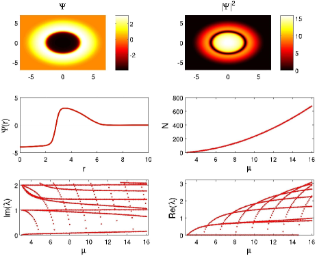
Figure 1: (Color online) Top panels: the RDS’ real-valued profile (left) and the corresponding density plot (right) for $\mu=16$. Middle left: a radial profile of the relevant state. Middle right: number of particles $N=\int|\psi|^{2}dr$ as a function of chemical potential $\mu$, showing the continuation of states from the linear limit to the nonlinear regime. Bottom panels: the imaginary (left) and real parts (right) of the spectrum; showcased is the generic instability of the RDS, and the emergence of additional unstable eigenmodes thereof as $\mu$ is increased. The value for the trap strength in this figure and all remaining figures is $\Omega=1$ (unless stated otherwise).

We now proceed to test these predictions, as well as to examine the BdG stability analysis and the dynamical evolution of the RDS, both in the absence (initially, for comparison and guidance) and then in the presence of the radial perturbation potential.

III Results

First, we briefly summarize the numerical techniques used in this work. Stationary states in both 1D (i.e., in a radial form) and 2D were identified using a centered finite-difference scheme within Newton’s method. The spectrum of the stationary states (i.e., the result of the BdG analysis) was calculated using the eigenvalue problem derived from Eq. (6). Finally, for the dynamics of the system, we used direct integration employing second order finite differences in space and fourth-order Runge-Kutta in time.

III.1 Basic properties of the ring dark soliton

Let us start by summarizing some of the basic properties of the RDS without the perturbation potential. A typical RDS state in the TF limit of large chemical potential $\mu$ is shown in the top and middle left panels of Fig. 1; the top right panel shows the corresponding density. As indicated in the previous section, the RDS has a linear limit (built out of the eigenstates of the 2D quantum harmonic oscillator). The continuation of such a state in the nonlinear regime is shown in the middle right panel of Fig. 1. The imaginary and real parts of the spectrum of the RDS are shown in the bottom panels of Fig. 1. Note that the RDS is unstable for any value of $\mu$ beyond the linear limit. More importantly, in line with what was also presented in Ref. middelphysd , as $\mu$ increases, more unstable modes keep emerging, through eigenvalue pairs that cross through the origin. These signal pitchfork bifurcations, to which we now turn.

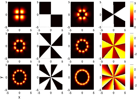
Figure 2: (Color online) The most unstable modes at a few representative chemical potential values $\mu=4$, 6, 9, 11, 14, and 16 (from left to right, top to bottom) associated with the instability of the RDS. Left and right subpanels correspond, respectively, to the absolute value and phase of the modes.

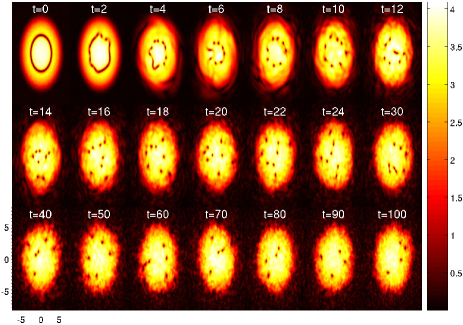
Figure 3: (Color online) Dynamics ensuing from the unstable RDS for $\mu=16$. Note that the RDS first deforms into seven pairs of vortices (in accordance with the most unstable mode for these parameters values; see the bottom right panel of Fig. 2), and then eventually turns into a dynamical evolving vortex cluster for longer times. During evolution, some of the vortices are “absorbed” by the BEC periphery and the system is eventually left with four interacting vortices.

Studies of RDS in atomic BECs have illustrated their dynamical breakup into vortex-antivortex pairs (see, e.g., Refs. rds2003 ; herring ). To complement this picture, we now discuss the most unstable modes of the BdG analysis. Some representative eigenmodes at $\mu=4,$ 6, 9, 11, 14 and 16 are shown in Fig. 2. It is interesting to observe that the identified modes indicate a clear connection to an increasing number of pairs of vortices. The first unstable mode appears to be connected to two-pairs, i.e., to a vortex quadrupole. Indeed, the vortex quadrupole exists as a state mottonen for any value of $\mu$ beyond the linear limit of $\mu=3\Omega$, being constructed as:

$$|\psi_{\rm{Q}}\rangle_{\rm{linear}}=\frac{|2,0\rangle+i|0,2\rangle}{\sqrt{2}}.$$ (16)

Subsequent destabilization modes reveal a three-fold symmetry (leading to the bifurcation of vortex hexagons middelphysd ), a four-fold symmetry (leading to vortex octagons), then a five-fold (decagons), a six-fold (dodecagons), and so on. These different eigenvectors are clearly illustrated in Fig. 2 and the existence and stability of the corresponding emerging (from the pitchfork bifurcation) vortex $n$-gon cluster states is discussed in Ref. annab .

A dynamical study of the states shows that the evolution initially results in vortex pairs, in agreement with Fig. 2. However, gradually some vortices may move out of the BEC and get lost in the background, leaving behind a complex, interacting cloud of vortices, as shown for $\mu=16$ in Fig. 3. The resulting interaction dynamics between vortices in the cluster, and the associated transfer of energies between different scales, may represent a very interesting setting for exploring turbulence phenomena and associated cascades in line, e.g., with recent experimental efforts of Ref. bpa_turb .

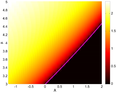
Figure 4: (Color online) Max$(|\Psi|)$ as a function of $(A,\mu)$. Note that $N$ decreases as $A$ increases when holding $\mu$ fixed until some critical set of values of $A$ (depicted by the purple line) beyond which the RDS will cease to exist. In the linear limit $\mu=3\Omega$, even a very small positive perturbation of $A$ will destroy the RDS state.

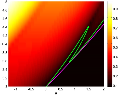
Figure 5: (Color online) Instability growth rate max(Re($\lambda$)) as a function of $(A,\mu)$. The area between the left (green) and right (purple) curves corresponds to the region where the RDS exists and with vanishing max(Re($\lambda$)), i.e. the RDS is completely stable. The rightmost purple line is also the boundary of the critical values of $A$ beyond which no RDS solution exists.

III.2 Adding the perturbation potential

Having analyzed the unperturbed case, we now examine the case with the radial Gaussian potential. The existence of the RDS structure in the latter case can be captured as a function of $(A,\mu)$ —see Fig. 4. We used max$(|\Psi|)$ (i.e., the max root density) as a diagnostic instead of $N$ for practical visualization purposes, in this case. We can see that for a fixed value of $\mu$, the density decreases as $A$ increases (a natural feature, given the repulsive nature of the perturbation potential) until a critical value of $A$ —shown as a purple line— is reached, beyond which the RDS will cease to exist. In the linear limit of $\mu=3\Omega$, even a very small positive perturbation of $A$ will destroy the RDS state. The monotonic dependence of $\mu$ on the critical $A$ appears to be approximately linear.

We proceed now with the central theme of this study, which is the dynamical stabilization of the RDS. To characterize the stability of the RDS in the $(A,\mu)$ plane, in Fig. 5 we show a plot of the max(Re($\lambda$)) as a function of $(A,\mu)$. The right most purple line, as before, depicts the critical values of $A$ beyond which no RDS solution exists. The region enclosed between the green and purple lines corresponds to the regimes where RDS exists with vanishing max(Re($\lambda$)), i.e., the RDS is completely stabilized by the presence of the external Gaussian ring perturbation potential. One interesting feature is that the relevant stability landscape is rather complex with potential sequences of destabilization and restabilization for values of $\mu\geq 3.6$ (we will return to this point below). However, the principal conclusion obtained from Fig. 5 is that the RDS is generically subject to full dynamical stabilization for any value of the chemical potential and for suitable intervals of the perturbation potential strength $A$ in the vicinity of the linear limit. The feature that the stabilization is enabled near the linear limit is rather natural to expect also on the basis of our earlier results for $A=0$ in Fig. 1. Given that the RDS is progressively more and more unstable (with a higher number of destabilizing modes) as $\mu$ increases suggests that the perturbation potential may be unable to suppress this multitude of unstable modes, especially far from the linear limit.

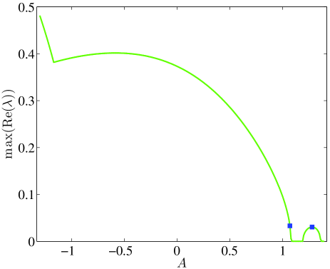
Figure 6: (Color online) Cross section of the instability growth rate max(Re($\lambda$)) at $\mu=4$. The right most point of the curve corresponds to the critical value of $A$ beyond which no RDS solution exists. The two blue squares are two points in two different instability regimes but with similar instability rates whose full spectrum is shown in Fig. 7.

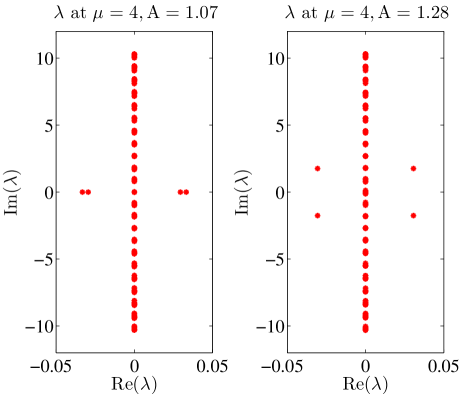
Figure 7: (Color online) Full stability spectrum corresponding to the two blue squares in the two different instability regimes in Fig. 6 for $\mu=4$. Left and right panels correspond to $A=1.07$ and $A=1.28$, respectively. Note that the two regimes do not share the same nature of instability. The large amplitude case (left) has the instability on the real axis (i.e., exponential instability) while the small amplitude case (right) has the instability in the form of a complex quartet (oscillatory instability).

To gain further insight on this stability plane, let us now study a typical cross section of Fig. 5 at $\mu=4$. The cross section is shown in Fig. 6. A detailed study of the full spectrum shows the existence of two intervals of instability which are not of the same nature. The leftmost interval (including $A=0$ in the absence of a defect) corresponds to a typically large(r) growth rate. Here, the instability derives from real eigenvalue pairs. Connecting with Fig. 1 and the case of $A=0$, we recognize that this unstable mode is associated with the breakup to vortex quadrupoles. As $A$ becomes increasingly more negative to the left of the figure, other modes may, in turn, dominate the instability dynamics (the “bend” in the stability diagram represents such a “take-over” of the dominant instability by a different mode; cf. Fig. 1). However, it is observed that as $A$ increases on the positive side, the unstable real pair(s) decrease in their real part and eventually cross through the origin of the spectral plane, becoming imaginary and hence stabilizing the RDS state. This is, once again, a key finding of our work, representing the RDS stabilization. However, as the (formerly unstable) eigenvalues bear a so-called ‘negative energy’, upon climbing up the imaginary axis, they may collide with eigenvalues associated with ‘positive energy’ modes (see, e.g., the discussion in pp. 56–58 of Ref. book2 ). This type of collision gives rise to a complex eigenvalue quartet and a different (weak) oscillatory dynamical instability, or a so-called Hamiltonian Hopf bifurcation; see, e.g., the discussion of Ref. goodman . The latter scenario leads to small instability bubbles, as the quartet may form, but subsequently the eigenvalues may return to the imaginary axis, splitting anew into two imaginary pairs.

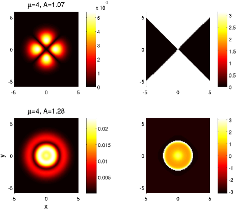
Figure 8: (Color online) The most unstable modes of Fig. 7. Top and bottom row of panels correspond, respectively, to the absolute value (left subpanels) and phase (right subpanels) of the solutions for the left and right cases depicted in Fig. 7.

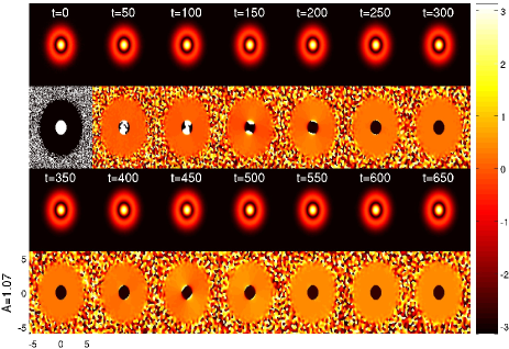
Figure 9: (Color online) Dynamics of the state in the top panels of Fig. 8. The odd panels depict the absolute value of the field while the even panels depict its phase. The state is oscillating between the vortex quadrupole and the RDS, but very weakly.

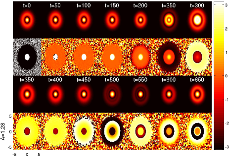
Figure 10: (Color online) The same plot as Fig. 9 but for the state in the bottom panels of Fig. 8. This state has a different nature of instability from the one in Fig. 9. The instability is like a vibrational mode.

The two (exponential and oscillatory) instability scenarios are illustrated in the two panels of Fig. 7 for smaller and larger values of $A$, respectively. The most unstable mode of each state is shown in Fig. 8, illustrating the distinct nature of the instability in the different scenarios. The state at $A=1.07$ is in the same branch of $A=-1,0$ and 1, and its instability leads to a deformation towards a vortex quadrupole state in a way similar as the first plot of Fig. 2. On the other hand, the state at $A=1.28$ appears to have a different type of instability that instead resembles a vibrational mode (the type of mode that could be captured through a ring particle model). The time dynamics of the two states are shown in Fig. 9 and Fig. 10 respectively. In the former case, we observe the recurrent formation of a vortex quadrupole (this is not immediately discernible in the density but distinctly visible in the phase pattern), in accordance with the identified unstable mode. In the latter, indeed unstable vibrational dynamical characteristics can be seen in the motion of the ring, which, however, appears to maintain its radial structure.

A different cross section of the stability plane of Fig. 5 is given in Fig. 11, now for the case of $A=0.5$, and varying the chemical potential $\mu$. From this perspective, we observe that $A$ delays the onset of instabilities as $\mu$ is increased. Another way to look at the effects of $A$ and $\mu$ is that $A$ plays effectively the opposite role to that of $\mu$: the increase of $A$ (for fixed $\mu$) drives the eigenmodes away from the real axis and into the imaginary axis while the increase of the chemical potential for fixed $A$ drives the eigenmodes away from the imaginary axis and into the real axis, causing instability. We believe that this discussion provides a unified perspective on the sources of destabilization and the potential for re-stabilization of the RDS.

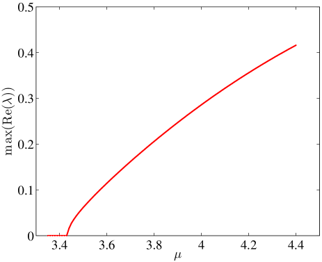
Figure 11: (Color online) Cross section of max(Re($\lambda$)) at $A=0.5$. The solution starts to exist around $\mu=3.35$. Note that $A$ delays the set in of instabilities as $\mu$ is increased.

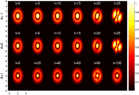
Figure 12: (Color online) Time evolution of states at $\mu=4$ with $A=-1$, 0 and 1 (top to bottom rows of panels). Note that the state of $A=1$ is significantly less unstable than those of $A=-1$ and $A=0$, which have roughly the same instability growth rate. Note also that all three states deform toward the vortex quadrupole state initially, although the third one maintains an oscillatory pattern between a recurring ring and a vortex quadrupole.

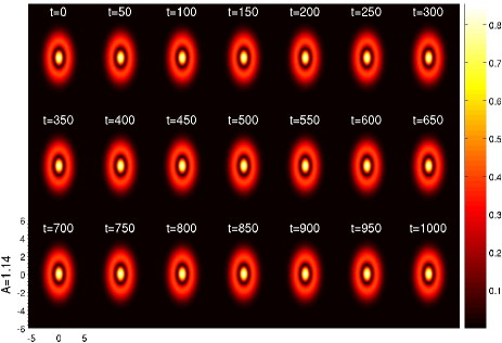
Figure 13: (Color online) Time evolution of states at $\mu=4$ with $A=1.14$ which is in a completely stable parametric interval. The state is shown to be stable up to t=1000, in agreement with our spectral results.

In all the cases considered, the stability conclusions were also found to be consonant with the corresponding dynamics, of which we now present a few additional case examples. In particular, we study the dynamical evolution of states at $\mu=4$ for different values of $A=-1,0,1$ (see Fig. 12) and $1.14$ (see Fig. 13) to probe the effects of the variation of $A$. Note that the cases of $A=-1$ and $0$ are about equally unstable at $\mu=4$ with $A=-1$ bearing a slightly larger growth rate. The case of $A=1$, however, is very close to, albeit not within the stabilization regime. On the other hand, the case of $A=1.14$ is fully stabilized. We add a random perturbation to the states, ensuring that the number of atoms in each case is, upon perturbation, 1.0013 times of the unperturbed one. The results of the dynamical evolution of the former three cases are shown in Fig. 12. Note that both states for $A=-1$ and $A=0$ are relatively quickly deformed around $t=25$ while the state for $A=1$ deforms only much later around $t=70$, due to its weaker growth rate. In all three cases, the states evolve initially towards the vortex quadrupole waveform. While the former two states will quickly deform afterwards and lose their radial structure, the third state can oscillate between the RDS state and the vortex quadrupole state for a much longer time at least up to $t=1000$. A dynamical evolution of states at $A=1.14$, which is in a completely stable parametric interval, is shown in Fig. 13. The state is shown to be stable at least up to $t=1000$, in agreement with the spectral findings and corroborating the full stabilization achieved by the presence of the Gaussian repulsive impurity.

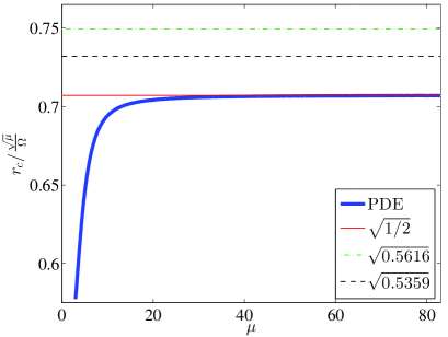
Figure 14: (Color online) The location of the RDS scaled by $\sqrt{\mu}/\Omega$ as a function of $\mu$ (thick solid blue line). Note that the numerical values reach a limiting value of $1/\sqrt{2}$ (thin horizontal solid red line) when $\mu$ is large. The particle picture can approximately describe the $\sqrt{\mu}$ behavior and over estimates $r_{c}$, but nevertheless is still an interesting approximate description of the RDS. The particle approach using the perturbed Lagrangian method [see Eqs. (8) and (9)] corresponds to the thin dotted-dash green line while the solvability condition for the steady state problem method [see Eq. (13)] is depicted by the thin dashed black line.

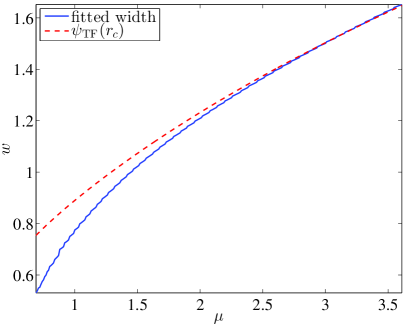
Figure 15: (Color online) Dark soliton width $w$ as a function of the chemical potential $\mu$. The blue solid line corresponds to fitting a profile $\psi_{\rm TF}(r)\times\tanh(\sqrt{w}(r-r_{c}))$ to the PDE steady state for $\Omega=0.2$. The red dashed line corresponds to the approximate value of the background at the location of the RDS, see Eq. (17).

III.3 The particle picture of the ring dark soliton

We first study how the equilibrium location $r_{c}$ of the RDS changes with chemical potential $\mu$, especially in the large density limit without the perturbation potential, and compare the numerical results and the particle picture predictions. Numerical results (for $\Omega=1$) suggest that $r_{c}=\sqrt{\mu/2}$ (see thin horizontal red line) in the large $\mu$ limit as shown in Fig. 14. As mentioned in Sec. II.2, a systematic analysis of Eqs. (8) and (9) yields the estimate $r_{c}=\sqrt{0.5616\mu}/\Omega$ (see horizontal thin dotted-dash green line). On the other hand, using the solvability condition for the steady state problem described in Sec. II.2, one obtains the better prediction of the RDS position $r_{c}=\sqrt{0.5359\mu}/\Omega$; see Eq. (13) and thin horizontal dashed black line in Fig. 14. It is important to mention that, although the above two particle approaches are able to capture the $\sqrt{\mu}/\Omega$ behavior of $r_{c}$, they do not lead to the precise numerical prefactor. This may be attributed to the choice of the ansatz (7), where the width of the stationary dark soliton is chosen to be $\sqrt{\mu}$. This selection corresponds to the width of a dark soliton in a homogeneous background of density $\mu$. However, due to the non-homogeneity of the BEC background, the RDS placed at $r_{c}$ experiences a background density $\mu_{0}$ which can be approximated using the TF regime (valid for large $\mu$) to be

$$\mu_{0}\approx\psi_{\rm TF}^{2}(r_{c})=\mu-V(r_{c})=\mu-\frac{1}{2}\Omega^{2}r_{c}^{2}.$$ (17)

For instance, in Fig. 15 we show an example where we extracted the width of the dark soliton for $\Omega=0.2$ as a function of $\mu$. As it is clear from the figure, as $\mu$ increases, the width of the dark soliton converges to $\sqrt{\mu_{0}}$ as prescribed in Eq. (17). Lastly, it is relevant to point out that, remarkably, the adiabatic invariant theory of Ref. kamch properly captures the asymptotic growth of the radius of the RDS as $\mu$ increases. It is for that reason that we will hereafter utilize the particle picture of Eq. (15) and Ref. kamch for our further static and dynamics considerations.

We now study the effect of $A$ on $r_{c}$. Figure 16 depicts $r_{c}$ as a function of $A$ for $\mu=24$. It is clear that the particle picture can capture the effect of $A$ fairly accurately. It is also observed that the critical radius decreases in comparison to the $A=0$ limit, in the presence of a repulsive defect, while the opposite is true in the case of an attractive defect.

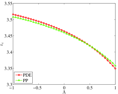
Figure 16: Position of the RDS as a function of $A$ for $\mu=24$. The (red) circles correspond to the full PDE dynamics and the (green) triangles to the particle picture (PP) described in Sec. II.2.

Finally, we study the radial oscillatory motion of the RDS in both the case bearing and in that without the perturbation potential. We initialize our displaced RDS state by superposing a suitable hyperbolic tangent profile to (i.e., multiplying it with) the numerically exact ground state at the same chemical potential $\mu=24$. Note that the RDS is unstable at such a high chemical potential, therefore, we can only simulate the PDE dynamics for a limited amount of time, before an instability leading to a polygonal cluster of vortices ensues. The comparison of the PDE and the particle picture dynamics for the cases of $A=0$ and $A=1$ are shown, respectively, in the top and bottom panels of Fig. 17. We see that the particle picture is able to capture the essential PDE radial oscillation dynamics both with and without the Gaussian barrier.

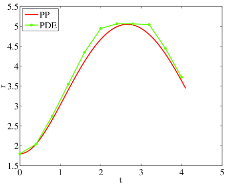
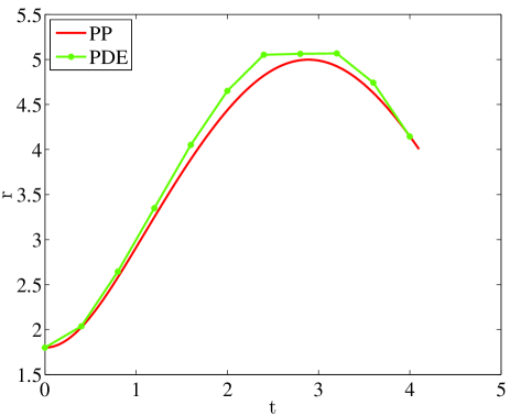
Figure 17: Radial oscillatory motion of the RDS with $\mu=24$ for $A=0$ and $A=1$. The central radius of the RDS is extracted from the PDE dynamics (green dots) and compared to the ODE evolution of the particle picture (PP, red line) according to Eq. (15).

IV Conclusions and Future Challenges

In this work, we studied the existence and stability of ring dark soliton states, initially in the absence and subsequently in the presence of a radially localized Gaussian perturbation potential. We have systematically shown, via a combination of spectral analysis and direct numerical simulations, that the ring dark soliton can be stabilized by adding the perturbation potential with a suitable strength, for all values of the chemical potential that we have considered herein. Our systematic spectral analysis has also revealed why this stabilization mechanism can only be effective near the linear limit of the system. It has also revealed the potential for secondary instabilities (due to pair collisions on the imaginary axis and complex eigenvalue quartets emerging from them) due to the excited state nature of the ring.

An additional effort, significantly motivated by the potential of the above method to lead to stable RDS vibrations, was that of deriving dynamical equations for their motion. We evaluated different techniques to this effect, showcasing the fact that although all approaches gave fairly similar results, the adiabatic invariant method of Ref. kamch presented a distinct advantage in capturing the radius of stationary rings. A self-consistent perturbative technique (based on earlier work in reaction-diffusion systems) was also adopted to that effect and was shown to give reasonably accurate results in its comparison with the full numerical results. Going beyond the “stationary particle” approach, allowing motion along the radial direction, an intriguing goal for the future may be to examine the ring soliton as a filamentary pattern embedded in 2D, which, in addition to radial internal modes, may possess bending ones (but without breaking). Such studies may in turn enable the observation of collisions and deformations of rings upon interactions, a topic that has been of interest also in nonlinear optics ektoras .

Finally, it may well be relevant to explore settings beyond the realm of two spatial dimensions, extending the present considerations to the case of 3D solitonic or vortex rings and other such patterns. Earlier work established how to construct such states in isotropic and anisotropic 3D limits starting from linear eigenstates craso2 . It is then of particular interest to continue such states in the nonlinear realm and explore their spectral and dynamical stability using tools similar to the ones proposed herein. Efforts along these directions are currently in progress and will be presented in future publications.

- (1) C. J. Pethick and H. Smith, Bose-Einstein Condensation in Dilute Gases (Cambridge University Press, Cambridge, 2008).
- (2) L. P. Pitaevskii and S. Stringari, Bose-Einstein Condensation (Oxford University Press, Oxford, 2003).
- (3) P. G. Kevrekidis, D. J. Frantzeskakis, and R. Carretero-González (eds.), Emergent Nonlinear Phenomena in Bose-Einstein Condensates. Theory and Experiment (Springer-Verlag, Berlin, 2008); R. Carretero-González, D. J. Frantzeskakis, and P. G. Kevrekidis, Nonlinearity 21, R139 (2008).
- (4) K. E. Strecker, G. B. Partridge, A. G. Truscott, and R. G. Hulet, Nature 417, 150 (2002).
- (5) L. Khaykovich, F. Schreck, G. Ferrari, T. Bourdel, J. Cubizolles, L. D. Carr, Y. Castin, and C. Salomon, Science 296, 1290 (2002).
- (6) S. L. Cornish, S. T. Thompson, and C. E. Wieman, Phys. Rev. Lett. 96, 170401 (2006).
- (7) D. J. Frantzeskakis, J. Phys. A 43, 213001 (2010).
- (8) B. Eiermann, Th. Anker, M. Albiez, M. Taglieber, P. Treutlein, K.-P. Marzlin, and M. K. Oberthaler, Phys. Rev. Lett. 92, 230401 (2004).
- (9) A. L. Fetter and A.A. Svidzinsky, J. Phys.: Cond. Mat. 13, R135 (2001).
- (10) A. L. Fetter, Rev. Mod. Phys. 81, 647 (2009).
- (11) S. Komineas, Eur. Phys. J.- Spec. Topics 147 133 (2007).
- (12) L. S. Leslie, A. Hansen, K. C. Wright, B. M. Deutsch, and N. P. Bigelow, Phys. Rev. Lett. 103, 250401 (2009).
- (13) M. W. Ray, E. Ruokokoski, S. Kandel, M. Möttönen, and D. S. Hall, Nature 505, 657 (2014).
- (14) S. Burger, K. Bongs, S. Dettmer, W. Ertmer, K. Sengstock, A. Sanpera, G. V. Shlyapnikov, and M. Lewenstein, Phys. Rev. Lett. 83, 5198 (1999).
- (15) J. Denschlag, J. E. Simsarian, D. L. Feder, C. W. Clark, L. A. Collins, J. Cubizolles, L. Deng, E. W. Hagley, K. Helmerson, W. P. Reinhardt, S. L. Rolston, B. I. Schneider, and W. D. Phillips, Science 287, 97 (2000).
- (16) Z. Dutton, M. Budde, C. Slowe, and L. V. Hau, Science 293, 663 (2001).
- (17) K. Bongs, S. Burger, S. Dettmer, D. Hellweg, J. Arlt, W. Ertmer, and K. Sengstock, C.R. Acad. Sci. Paris 2, 671 (2001).
- (18) B. P. Anderson, P. C. Haljan, C. A. Regal, D. L. Feder, L. A. Collins, C. W. Clark, and E. A. Cornell, Phys. Rev. Lett. 86, 2926 (2001).
- (19) P. Engels and C. Atherton, Phys. Rev. Lett. 99, 160405 (2007).
- (20) C. Becker, S. Stellmer, P. Soltan-Panahi, S. Dörscher, M. Baumert, E.-M. Richter, J. Kronjäger, K. Bongs, and K. Sengstock, Nature Phys. 4, 496 (2008).
- (21) S. Stellmer, C. Becker, P. Soltan-Panahi, E.-M. Richter, S. Dörscher, M. Baumert, J. Kronjäger, K. Bongs, and K. Sengstock, Phys. Rev. Lett. 101, 120406 (2008).
- (22) A. Weller, J. P. Ronzheimer, C. Gross, J. Esteve, M. K. Oberthaler, D. J. Frantzeskakis, G. Theocharis, and P. G. Kevrekidis, Phys. Rev. Lett. 101, 130401 (2008).
- (23) G. Theocharis, A. Weller, J. P. Ronzheimer, C. Gross, M. K. Oberthaler, P. G. Kevrekidis, and D. J. Frantzeskakis, Phys. Rev. A 81, 063604 (2010).
- (24) I. Shomroni, E. Lahoud, S. Levy, and J. Steinhauer, Nat. Phys. 5, 193 (2009).
- (25) C. Becker, K. Sengstock, P. Schmelcher, P. G. Kevrekidis, and R. Carretero-González, New J. Phys. 15, 113028 (2013).
- (26) M. Ma, R. Carretero-González, P. G. Kevrekidis, D. J. Frantzeskakis, and B. A. Malomed, Phys. Rev. A 82, 023621 (2010).
- (27) Yu.S. Kivshar and X. Yang, Phys. Rev. E 50, R40 (1994).
- (28) A. Dreischuh, V. Kamenov, and S. Dinev, Appl. Phys. B 62, 139 (1996);
- (29) D. J. Frantzeskakis and B. A. Malomed, Phys. Lett. A 264, 179 (1999).
- (30) H. E. Nistazakis, D. J. Frantzeskakis, B. A. Malomed, and P. G. Kevrekidis, Phys. Lett. A 285, 157 (2001).
- (31) Jie-Fang Zhang, Lei Wu, Lu Li, D. Mihalache, and B. A. Malomed, Phys. Rev. A 81, 023836 (2010); G. J. de Valcárcel and K. Staliunas Phys. Rev. A 87, 043802 (2013).
- (32) D. Neshev, A. Dreischuh, V. Kamenov, I. Stefanov, S. Dinev, W. Fliesser, and L. Windholz, Appl. Phys. B 64, 429 (1997); A. Dreischuh, D. Neshev, G. G. Paulus, F. Grasbon, and H. Walther, Phys. Rev. E 66, 066611 (2002).
- (33) G. Theocharis, D. J. Frantzeskakis, P. G. Kevrekidis, B. A. Malomed, and Yu. S. Kivshar, Phys. Rev. Lett. 90, 120403 (2003).
- (34) L. D. Carr and C. W. Clark, Phys. Rev. A 74, 043613 (2006).
- (35) A. M. Kamchatnov and S. V. Korneev, Phys. Lett. A 374, 4625 (2010).
- (36) L. A. Toikka, J. Hietarinta, and K.-A. Suominen, J. Phys. A 45, 485203 (2012).
- (37) Shi-Jie Yang, Quan-Sheng Wu, Sheng-Nan Zhang, Shiping Feng, Wenan Guo, Yu-Chuan Wen, and Yue Yu, Phys. Rev. A 76, 063606 (2007); Shi-Jie Yang, Quan-Sheng Wu, Shiping Feng, Yu-Chuan Wen, and Yue Yu, Phys. Rev. A 77, 035602 (2008); L. A. Toikka, New J. Phys. 16, 043011 (2014); L. A. Toikka, O. Kärki, and K.-A. Suominen, J. Phys. B 47, 021002 (2014).
- (38) Shu-Wei Song, Deng-Shan Wang, Hanquan Wang, and W. M. Liu Phys. Rev. A 85, 063617 (2012).
- (39) G. Herring, L. D. Carr, R. Carretero-González, P. G. Kevrekidis, and D. J. Frantzeskakis, Phys. Rev. A 77, 023625 (2008).
- (40) J. Stockhofe, P. G. Kevrekidis, D. J. Frantzeskakis, and P. Schmelcher, J. Phys. B 44, 191003 (2011).
- (41) Th. Busch and J. R. Anglin, Phys. Rev. Lett. 87, 010401 (2001).
- (42) C. Becker, S. Stellmer, P. Soltan-Panahi, S. Dörscher, M. Baumert, E.-M. Richter, J. Kronjäger, K. Bongs, and K. Sengstock, Nature Phys. 4, 496 (2008).
- (43) S. Middelkamp, J. J. Chang, C. Hamner, R. Carretero-González, P. G. Kevrekidis, V. Achilleos, D. J. Frantzeskakis, P. Schmelcher, and P. Engels, Phys. Lett. A 375, 642 (2011).
- (44) C. Hamner, J. J. Chang, P. Engels, M. A. Hoefer, Phys. Rev. Lett. 106, 065302 (2011).
- (45) P. G. Kevrekidis, G. Theocharis, D. J. Frantzeskakis, and B. A. Malomed Phys. Rev. Lett. 90, 230401 (2003).
- (46) Shi-Jie Yang, Quan-Sheng Wu, Shiping Feng, Yu-Chuan Wen, and Yue Yu Phys. Rev. A 77, 035602 (2008).
- (47) S. Middelkamp, P. G. Kevrekidis, D. J. Frantzeskakis, R. Carretero-González, and P. Schmelcher, Physica D 240, 1449 (2011).
- (48) K. C. Wright, R. B. Blakestad, C. J. Lobb, W. D. Phillips, and G. K. Campbell, Phys. Rev. Lett. 110, 025302 (2013); S. Eckel, J. G. Lee, F. Jendrzejewski, N. Murray, C. W. Clark, C. J. Lobb, W. D. Phillips, M. Edwards, and G. K. Campbell, Nature 506, 200 (2014).
- (49) K. Henderson, C. Ryu, C. MacCormick and M.G. Boshier, New J. Phys. 11, 043030 (2009); C. Ryu, P.W. Blackburn, A.A. Blinova and M.G. Boshier, Phys. Rev. Lett. 111, 205301 (2013).
- (50) T. Kapitula, P. G. Kevrekidis, and R. Carretero-González. Physica D 233, 112 (2007).
- (51) A. S. Rodrigues, P. G. Kevrekidis, R. Carretero-González, J. Cuevas-Maraver, D. J. Frantzeskakis, and F. Palmero, J. Phys.: Cond. Mat. 26, 155801 (2014).
- (52) L. Dominici, D. Ballarini, M. De Giorgi, E. Cancellieri, B. Silva Fernández, A. Bramati, G. Gigli, F. Laussy, D. Sanvitto, arXiv:1309.3083.
- (53) G. Theocharis, P. Schmelcher, M. K. Oberthaler, P. G. Kevrekidis, and D. J. Frantzeskakis, Phys. Rev. A 72, 023609 (2005).
- (54) D. S. Morgan and T. J. Kaper, Physica D 192, 33 (2004).
- (55) J. Guckenheimer and P. J. Holmes, Nonlinear Oscillations, Dynamical Systems, and Bifurcations of Vector Fields (Springer, Berlin, 1983).
- (56) L. C. Crasovan, G. Molina-Terriza, J. P. Torres, L. Torner, V. M. Pérez-García, and D. Mihalache, Phys. Rev. E 66, 036612 (2002); M. Möttönen, S. M. M. Virtanen, T. Isoshima, and M. M. Salomaa, Phys. Rev. A 71, 033626 (2005); S. Middelkamp, P. G. Kevrekidis, D. J. Frantzeskakis, R. Carretero-González, and P. Schmelcher, Phys. Rev. A 82, 013646 (2010).
- (57) A. M. Barry and P. G. Kevrekidis, J. Phys. A 46, 445001 (2013).
- (58) T. W. Neely, A. S. Bradley, E. C. Samson, S. J. Rooney, E. M. Wright, K. J. H. Law, R. Carretero-González, P. G. Kevrekidis, M. J. Davis, and B. P. Anderson, Phys. Rev. Lett. 111, 235301 (2013).
- (59) R. H. Goodman, J. Phys. A 44, 425101 (2011).
- (60) L.-C. Crasovan, V. M. Pérez-García, I. Danaila, D. Mihalache, L. Torner, Phys. Rev. A 70, 033605 (2004).