Learning and Forecasting Opinion Dynamics in Social Networks

Abir De IIT Kharagpur, {abir.de, niloy, sourangshu}@cse.iitkgp.ernet.in Isabel Valera Max Plank Institute for Software Systems, {ivalera, manuelgr}@mpi-sws.org Niloy Ganguly IIT Kharagpur, {abir.de, niloy, sourangshu}@cse.iitkgp.ernet.in Sourangshu Bhattacharya IIT Kharagpur, {abir.de, niloy, sourangshu}@cse.iitkgp.ernet.in Manuel Gomez-Rodriguez Max Plank Institute for Software Systems, {ivalera, manuelgr}@mpi-sws.org
Abstract

Social media and social networking sites have become a global pinboard for exposition and discussion of news, topics, and ideas, where social media users often update their opinions about a particular topic by learning from the opinions shared by their friends. In this context, can we learn a data-driven model of opinion dynamics that is able to accurately forecast users’ opinions? In this paper, we introduce SLANT, a probabilistic modeling framework of opinion dynamics, which represents users’ opinions over time by means of marked jump diffusion stochastic differential equations, and allows for efficient model simulation and parameter estimation from historical fine grained event data. We then leverage our framework to derive a set of efficient predictive formulas for opinion forecasting and identify conditions under which opinions converge to a steady state. Experiments on data gathered from Twitter show that our model provides a good fit to the data and our formulas achieve more accurate forecasting than alternatives.

1 Introduction

Social media and social networking sites are increasingly used by people to express their opinions, give their “hot takes”, on the latest breaking news, political issues, sports events, and new products. As a consequence, there has been an increasing interest on leveraging social media and social networking sites to sense and forecast opinions, as well as understand opinion dynamics. For example, political parties routinely use social media to sense people’s opinion about their political discourse111{http://www.nytimes.com/2012/10/08/technology/campaigns-use-social-media-to-lure-younger-voters.html}; quantitative investment firms measure investor sentiment and trade using social media [17]; and, corporations leverage brand sentiment, estimated from users’ posts, likes and shares in social media and social networking sites, to design their marketing campaigns222http://www.nytimes.com/2012/07/31/technology/facebook-twitter-and-foursquare-as-corporate-focus-groups.html. In this context, multiple methods for sensing opinions, typically based on sentiment analysis [20], have been proposed in recent years. However, methods for accurately forecasting opinions are still scarce [6, 7, 18], despite the extensive literature on theoretical models of opinion dynamics [5, 8].

In this paper, we develop a novel modeling framework of opinion dynamics in social media and social networking sites, SLANT 333Slant is a particular point of view from which something is seen or presented., which allows for accurate forecasting of individual users’ opinions. The proposed framework is based on two simple intuitive ideas: i) users’ opinions are hidden until they decide to share it with their friends (or neighbors); and, ii) users may update their opinions about a particular topic by learning from the opinions shared by their friends. While the latter is one of the main underlying premises used by many well-known theoretical models of opinion dynamics [5, 8, 21], the former has been ignored by models of opinion dynamics, despite its relevance on closely related processes such as information diffusion [11].

More in detail, our proposed model represents users’ latent opinions as continuous-time stochastic processes driven by a set of marked jump stochastic differential equations (SDEs) [13]. Such construction allows each user’s latent opinion to be modulated over time by the opinions asynchronously expressed by her neighbors as sentiment messages. Here, every time a user expresses an opinion by posting a sentiment message, she reveals a noisy estimate of her current latent opinion. Then, we exploit a key property of our model, the Markov property, to develop:

  • I.

    An efficient estimation procedure to find the parameters that maximize the likelihood of a set of (millions of) sentiment messages via convex programming.

  • II.

    A scalable simulation procedure to sample millions of sentiment messages from the proposed model in a matter of minutes.

  • III.

    A set of novel predictive formulas for efficient and accurate opinion forecasting, which can also be used to identify conditions under which opinions converge to a steady state of consensus or polarization.

Finally, we experiment on both synthetic and real data gathered from Twitter and show that our model provides a good fit to the data and our predictive formulas achieve more accurate opinion forecasting than several alternatives [6, 7, 8, 14, 25].

Related work. There is an extensive line of work on theoretical models of opinion dynamics and opinion formation [3, 5, 8, 14, 16, 25]. However, previous models typically share the following limitations: (i) they do not distinguish between latent opinion and sentiment (or expressed opinion), which is a noisy observation of the opinion (e.g., thumbs up/down, text sentiment); (ii) they consider users’ opinions to be updated synchronously in discrete time, however, opinions may be updated asynchronously following complex temporal patterns [11]; (iii) the model parameters are difficult to learn from real fine-grained data and instead are set arbitrarily, as a consequence, they provide inaccurate fine-grained predictions; and, (iv) they focus on analyzing only the steady state of the users’ opinions, neglecting the transient behavior of real opinion dynamics which allows for opinion forecasting methods. More recently, there have been some efforts on designing models that overcome some of the above limitations and provide more accurate predictions [6, 7]. However, they do not distinguish between opinion and sentiment and still consider opinions to be updated synchronously in discrete time. Our modeling framework addresses the above limitations and, by doing so, achieves more accurate opinion forecasting than alternatives.

2 Proposed model

In this section, we first formulate our model of opinion dynamics, starting from the data it is designed for, and then introduce efficient methods for model parameter estimation and model simulation.

Opinions data. Given a directed social network 𝒢=(𝒱,)𝒢𝒱\mathcal{G}=(\mathcal{V},\mathcal{E}), we record each message as e:=(u,m,t)assign𝑒𝑢𝑚𝑡e:=(u,m,t), where the triplet means that the user u𝒱𝑢𝒱u\in\mathcal{V} posted a message with sentiment m𝑚m at time t𝑡t. Given a collection of messages {e1=(u1,m1,t1),,en=(un,mn,tn)}formulae-sequencesubscript𝑒1subscript𝑢1subscript𝑚1subscript𝑡1subscript𝑒𝑛subscript𝑢𝑛subscript𝑚𝑛subscript𝑡𝑛\{e_{1}=(u_{1},m_{1},t_{1}),\ldots,e_{n}=(u_{n},m_{n},t_{n})\}, the history u(t)subscript𝑢𝑡\mathcal{H}_{u}(t) gathers all messages posted by user u𝑢u up to but not including time t𝑡t, i.e.,

u(t)={ei=(ui,mi,ti)|ui=uandti<t},subscript𝑢𝑡conditional-setsubscript𝑒𝑖subscript𝑢𝑖subscript𝑚𝑖subscript𝑡𝑖subscript𝑢𝑖𝑢andsubscript𝑡𝑖𝑡\mathcal{H}_{u}(t)=\{e_{i}=(u_{i},m_{i},t_{i})|u_{i}=u\ \mbox{and}\,t_{i}<t\}, (1)

and (t):=u𝒱u(t)assign𝑡subscript𝑢𝒱subscript𝑢𝑡\mathcal{H}(t):=\cup_{u\in\mathcal{V}}\mathcal{H}_{u}(t) denotes the entire history of messages up to but not including time t𝑡t.

Generative process. We represent users’ latent opinions as a multidimensional stochastic process 𝐱(t)superscript𝐱𝑡\mathbf{x}^{*}(t), in which the u𝑢u-th entry, xu(t)subscriptsuperscript𝑥𝑢𝑡x^{*}_{u}(t)\in\mathbb{R}, represents the opinion of user u𝑢u at time t𝑡t and the sign means that it may depend on the history (t)𝑡\mathcal{H}(t). Then, every time a user u𝑢u posts a message at time t𝑡t, we draw its sentiment m𝑚m from a sentiment distribution p(m|xu(t))𝑝conditional𝑚subscriptsuperscript𝑥𝑢𝑡p(m|x^{*}_{u}(t)). Here, we can also think of the sentiment m𝑚m of each message as samples from a noisy stochastic process mu(t)p(mu(t)|xu(t))similar-tosubscript𝑚𝑢𝑡𝑝conditionalsubscript𝑚𝑢𝑡subscriptsuperscript𝑥𝑢𝑡m_{u}(t)\sim p(m_{u}(t)|x^{*}_{u}(t)). Further, we represent the message times by a set of counting processes. In particular, we denote the set of counting processes as a vector 𝑵(t)𝑵𝑡\bm{N}(t), in which the u𝑢u-th entry, Nu(t){0}+subscript𝑁𝑢𝑡0superscriptN_{u}(t)\in\left\{0\right\}\cup\mathbb{Z}^{+}, counts the number of sentiment messages user u𝑢u posted up to but not including time t𝑡t. Then, we can characterize the message rate of the users using their corresponding conditional intensities as

𝔼[d𝑵(t)|(t)]=𝝀(t)dt,𝔼delimited-[]conditional𝑑𝑵𝑡𝑡superscript𝝀𝑡𝑑𝑡\mathbb{E}[d\bm{N}(t)\,|\,\mathcal{H}(t)]=\boldsymbol{\lambda}^{*}(t)\,dt, (2)

where d𝑵(t):=(dNu(t))u𝒱assign𝑑𝑵𝑡subscript𝑑subscript𝑁𝑢𝑡𝑢𝒱d\bm{N}(t):=\left(~{}dN_{u}(t)~{}\right)_{u\in\mathcal{V}} denotes the number of messages per user in the window [t,t+dt)𝑡𝑡𝑑𝑡[t,t+dt) and 𝝀(t):=(λu(t))u𝒱assignsuperscript𝝀𝑡subscriptsuperscriptsubscript𝜆𝑢𝑡𝑢𝒱\boldsymbol{\lambda}^{*}(t):=(~{}\lambda_{u}^{*}(t)~{})_{u\in\mathcal{V}} denotes the associated user intensities, which may depend on the history (t)𝑡\mathcal{H}(t). We denote the set of user that u𝑢u follows by 𝒩(u)𝒩𝑢\mathcal{N}(u). Next, we specify the the intensity functions 𝝀(t)superscript𝝀𝑡\boldsymbol{\lambda}^{*}(t), the dynamics of the users’ opinions 𝐱(t)superscript𝐱𝑡\mathbf{x}^{*}(t), and the sentiment distribution p(m|xu(t))𝑝conditional𝑚subscriptsuperscript𝑥𝑢𝑡p(m|x^{*}_{u}(t)).

Intensity for messages. There is a wide variety of message intensity functions one can choose from to model the users’ intensity 𝝀(t)superscript𝝀𝑡\boldsymbol{\lambda}^{*}(t) [1]. In this work, we consider two of the most popular functional forms used in the growing literature on social activity modeling using point processes [9, 23]:

  • I.

    Poisson process. The intensity is assumed to be independent of the history (t)𝑡\mathcal{H}(t) and constant, i.e., λu(t)=μusuperscriptsubscript𝜆𝑢𝑡subscript𝜇𝑢\lambda_{u}^{*}(t)=\mu_{u}.

  • II.

    Multivariate Hawkes processes. The intensity captures a mutual excitation phenomena between message events and depends on the whole history of message events v{u𝒩(u)}v(t)subscript𝑣𝑢𝒩𝑢subscript𝑣𝑡\cup_{v\in\{u\cup\mathcal{N}(u)\}}\mathcal{H}_{v}(t) before t𝑡t:

    λu(t)=μu+vu𝒩(u)bvueiv(t)κ(tti)=μu+vu𝒩(u)bvu(κ(t)dNv(t)),subscriptsuperscript𝜆𝑢𝑡subscript𝜇𝑢subscript𝑣𝑢𝒩𝑢subscript𝑏𝑣𝑢subscriptsubscript𝑒𝑖subscript𝑣𝑡𝜅𝑡subscript𝑡𝑖subscript𝜇𝑢subscript𝑣𝑢𝒩𝑢subscript𝑏𝑣𝑢𝜅𝑡𝑑subscript𝑁𝑣𝑡\lambda^{*}_{u}(t)=\mu_{u}+\sum_{v\in u\cup\mathcal{N}(u)}b_{vu}\sum_{e_{i}\in\mathcal{H}_{v}(t)}\kappa(t-t_{i})=\mu_{u}+\sum_{v\in u\cup\mathcal{N}(u)}b_{vu}~{}(\kappa(t)\star dN_{v}(t)), (3)

    where the first term, μu0subscript𝜇𝑢0\mu_{u}\geqslant 0, models the publication of messages by user u𝑢u on her own initiative, and the second term, with bvu0subscript𝑏𝑣𝑢0b_{vu}\geqslant 0, models the publication of additional messages by user u𝑢u due to the influence that previous messages posted by the users she follows have on her intensity. Here, κ(t)=eνt𝜅𝑡superscript𝑒𝜈𝑡\kappa(t)=e^{\nu t} is an exponential triggering kernel modeling the decay of influence of the past events over time and \star denotes the convolution operation.

In both cases, the couple (𝑵(t),𝝀(t))𝑵𝑡superscript𝝀𝑡(\bm{N}(t),\boldsymbol{\lambda}^{*}(t)) is a Markov process, i.e., future states of the process (conditional on past and present states) depends only upon the present state, and we can express the users’ intensity more compactly using the following jump stochastic differential equation (SDE):

d𝝀(t)=ν(𝝁𝝀(t))dt+𝐁d𝑵(t),𝑑superscript𝝀𝑡𝜈𝝁superscript𝝀𝑡𝑑𝑡𝐁𝑑𝑵𝑡d\boldsymbol{\lambda}^{*}(t)=\nu(\boldsymbol{\mu}-\boldsymbol{\lambda}^{*}(t))dt+\mathbf{B}d\bm{N}(t),

where the initial condition is 𝝀(0)=𝝁superscript𝝀0𝝁\boldsymbol{\lambda}^{*}(0)=\boldsymbol{\mu}. The Markov property will become important later.

Stochastic process for opinion. The opinion xu(t)subscriptsuperscript𝑥𝑢𝑡x^{*}_{u}(t) of a user u𝑢u at time t𝑡t adopts the following form:

xu(t)=αu+v𝒩(u)avueiv(t)mig(tti)=αu+v𝒩(u)avu(g(t)(mv(t)dNv(t))),subscriptsuperscript𝑥𝑢𝑡subscript𝛼𝑢subscript𝑣𝒩𝑢subscript𝑎𝑣𝑢subscriptsubscript𝑒𝑖subscript𝑣𝑡subscript𝑚𝑖𝑔𝑡subscript𝑡𝑖subscript𝛼𝑢subscript𝑣𝒩𝑢subscript𝑎𝑣𝑢𝑔𝑡subscript𝑚𝑣𝑡𝑑subscript𝑁𝑣𝑡x^{*}_{u}(t)=\alpha_{u}+\sum_{v\in\mathcal{N}(u)}a_{vu}\sum_{e_{i}\in\mathcal{H}_{v}(t)}m_{i}g(t-t_{i})=\alpha_{u}+\sum_{v\in\mathcal{N}(u)}a_{vu}~{}(g(t)\star(m_{v}(t)dN_{v}(t))), (4)

where the first term, αusubscript𝛼𝑢\alpha_{u}\in\mathbb{R}, models the original opinion a user u𝑢u starts with, the second term, with avusubscript𝑎𝑣𝑢a_{vu}\in\mathbb{R}, models updates in user u𝑢u’s opinion due to the influence that previous messages with opinions misubscript𝑚𝑖m_{i} posted by the users u𝑢u follows has on her opinion. Here, g(t)=eωt𝑔𝑡superscript𝑒𝜔𝑡g(t)=e^{-\omega t} denotes an exponential triggering kernel, which models the decay of influence over time.

Under this form, the resulting opinion dynamics are Markovian and can be compactly represented by a set of coupled marked jumped stochastic differential equations (proven in Appendix A):

Proposition 1.

The tuple (𝐱(t),𝛌(t),𝐍(t))superscript𝐱𝑡superscript𝛌𝑡𝐍𝑡(\mathbf{x}^{*}(t),\boldsymbol{\lambda}^{*}(t),\bm{N}(t)) is a Markov process, whose dynamics are defined by the following marked jumped stochastic differential equations (SDE):

d𝐱(t)𝑑superscript𝐱𝑡\displaystyle d\mathbf{x}^{*}(t) =ω(𝜶𝐱(t))dt+𝐀(𝐦(t)d𝑵(t))absent𝜔𝜶superscript𝐱𝑡𝑑𝑡𝐀direct-product𝐦𝑡𝑑𝑵𝑡\displaystyle=\omega(\boldsymbol{\alpha}-\mathbf{x}^{*}(t))dt+\mathbf{A}(\mathbf{m}(t)\odot d\bm{N}(t)) (5)
d𝝀(t)𝑑superscript𝝀𝑡\displaystyle d\boldsymbol{\lambda}^{*}(t) =ν(𝝁𝝀(t))dt+𝐁d𝑵(t)absent𝜈𝝁superscript𝝀𝑡𝑑𝑡𝐁𝑑𝑵𝑡\displaystyle=\nu(\boldsymbol{\mu}-\boldsymbol{\lambda}^{*}(t))dt+\mathbf{B}\,d\bm{N}(t) (6)

where the initial conditions are 𝛌(0)=𝛍superscript𝛌0𝛍\boldsymbol{\lambda}^{*}(0)=\boldsymbol{\mu} and 𝐱(0)=𝛂superscript𝐱0𝛂\mathbf{x}^{*}(0)=\boldsymbol{\alpha}, the marks are the sentiment messages 𝐦(t)=(mu(t))u𝒱𝐦𝑡subscriptsubscript𝑚𝑢𝑡𝑢𝒱\mathbf{m}(t)=\left(~{}m_{u}(t)~{}\right)_{u\in\mathcal{V}}, with mu(t)p(m|xu(t))similar-tosubscript𝑚𝑢𝑡𝑝conditional𝑚subscriptsuperscript𝑥𝑢𝑡m_{u}(t)\sim p(m|x^{*}_{u}(t)), and the sign direct-product\odot denotes pointwise product.

The above mentioned Markov property will be the key to the design of efficient model parameter estimation and model simulation algorithms.

Sentiment distribution. The particular choice of sentiment distribution p(m|xu(t))𝑝conditional𝑚subscriptsuperscript𝑥𝑢𝑡p(m|x^{*}_{u}(t)) depends on the recorded marks. For example, one may consider:

  • I.

    Gaussian Distribution The sentiment is assumed to be a real random variable m𝑚m\in\mathbb{R}, i.e., p(m|xu(t))=𝒩(xu(t),σu)𝑝conditional𝑚subscript𝑥𝑢𝑡𝒩subscript𝑥𝑢𝑡subscript𝜎𝑢p(m|x_{u}(t))=\mathcal{N}(x_{u}(t),\sigma_{u}). This fits well scenarios in which sentiment is extracted from text using sentiment analysis [12].

  • II.

    Logistic. The sentiment is assumed to be a binary random variable m{1,1}𝑚11m\in\{-1,1\}, i.e., p(m|xu(t))=1/(1+exp(mxu(t)))𝑝conditional𝑚subscript𝑥𝑢𝑡11𝑚subscript𝑥𝑢𝑡p(m|x_{u}(t))=1/(1+\exp(-m\cdot x_{u}(t))). This fits well scenarios in which sentiment is measured by means of up votes, down votes or likes.

Our model estimation method can be easily adapted to any log-concave sentiment distribution. However, in the remainder of the paper, we consider the Gaussian distribution since, in our experiments, sentiment is extracted from text using sentiment analysis.

2.1 Model parameter estimation

Given a collection of messages (T)={(ui,mi,ti)}𝑇subscript𝑢𝑖subscript𝑚𝑖subscript𝑡𝑖\mathcal{H}(T)=\{(u_{i},m_{i},t_{i})\} recorded during a time period [0,T)0𝑇[0,T) in a social network 𝒢=(𝒱,)𝒢𝒱\mathcal{G}=(\mathcal{V},\mathcal{E}), we can find the optimal parameters 𝜶𝜶\boldsymbol{\alpha}, 𝝁𝝁\boldsymbol{\mu}, 𝑨𝑨\bm{A} and 𝑩𝑩\bm{B} by solving a maximum likelihood estimation (MLE) problem444Here, if one decides to model the message intensities with a Poisson process, 𝑩=0𝑩0\bm{B}=0.. To do so, it is easy to show that the log-likelihood of the messages is given by

(𝜶,𝝁,𝑨,𝑩)=ei(T)logp(mi|xui(ti))message sentiments+ei(T)logλui(ti)u𝒱0Tλu(τ)𝑑τmessage times.𝜶𝝁𝑨𝑩subscriptsubscriptsubscript𝑒𝑖𝑇𝑝conditionalsubscript𝑚𝑖subscriptsuperscript𝑥subscript𝑢𝑖subscript𝑡𝑖message sentimentssubscriptsubscriptsubscript𝑒𝑖𝑇superscriptsubscript𝜆subscript𝑢𝑖subscript𝑡𝑖subscript𝑢𝒱superscriptsubscript0𝑇superscriptsubscript𝜆𝑢𝜏differential-d𝜏message times\mathcal{L}(\boldsymbol{\alpha},\boldsymbol{\mu},\bm{A},\bm{B})=\underbrace{\sum_{e_{i}\in\mathcal{H}(T)}\log p(m_{i}|x^{*}_{u_{i}}(t_{i}))}_{\text{message sentiments}}+\underbrace{\sum_{e_{i}\in\mathcal{H}(T)}\log\lambda_{u_{i}}^{*}(t_{i})-\sum_{u\in\mathcal{V}}\int_{0}^{T}\lambda_{u}^{*}(\tau)\,d\tau}_{\text{message times}}. (7)

Then, we can find the optimal parameters (𝜶,𝝁,𝑨,𝑩)𝜶𝝁𝑨𝑩(\boldsymbol{\alpha},\boldsymbol{\mu},\bm{A},\bm{B}) using MLE as

maximize𝜶,𝝁0,𝑨,𝑩0formulae-sequence𝜶𝝁0𝑨𝑩0maximize\displaystyle\underset{\boldsymbol{\alpha},\boldsymbol{\mu}\geq 0,\bm{A},\bm{B}\geq 0}{\text{maximize}} (𝜶,𝝁,𝑨,𝑩).𝜶𝝁𝑨𝑩\displaystyle\mathcal{L}(\boldsymbol{\alpha},\boldsymbol{\mu},\bm{A},\bm{B}). (8)

Note that, as long as the sentiment distributions are log-concave, the MLE problem above is concave and thus can be solved efficiently. Moreover, the problem decomposes in 2|𝒱|2𝒱2|\mathcal{V}| independent subproblems, two per user u𝑢u, since the first term in Eq. 7 only depends on (𝜶,𝑨)𝜶𝑨(\boldsymbol{\alpha},\bm{A}) whereas the last two terms only depend on (𝝁,𝑩)𝝁𝑩(\boldsymbol{\mu},\bm{B}), and thus can be readily parallelized. Then, we find (𝝁,𝑩)superscript𝝁superscript𝑩(\boldsymbol{\mu}^{*},\bm{B}^{*}) using spectral projected gradient descent [4], which works well in practice and achieves ε𝜀\varepsilon accuracy in O(log(1/ε))𝑂1𝜀O(\log(1/\varepsilon)) iterations, and find (𝜶,𝑨)superscript𝜶superscript𝑨(\boldsymbol{\alpha}^{*},\bm{A}^{*}) analytically, since, for Gaussian sentiment distributions, the problem reduces to a least-square problem. Fortunately, in each subproblem, we can use the Markov property from Proposition 1 to precompute the sums and integrals in (8) in linear time, i.e., O(|u(T)|+|v𝒩(u)v(T)|)𝑂subscript𝑢𝑇subscript𝑣𝒩𝑢subscript𝑣𝑇O(|\mathcal{H}_{u}(T)|+|\cup_{v\in\mathcal{N}(u)}\mathcal{H}_{v}(T)|). Appendix H summarizes the overall estimation algorithm.

2.2 Model simulation

We leverage the efficient sampling algorithm for multivariate Hawkes introduced by Farajtabar et al. [10] to design a scalable algorithm to sample opinions from our model. The two key ideas that allow us to adapt the procedure by Farajtabar et al. to our model of opinion dynamics, while keeping its efficiency, are as follows: (i) the opinion dynamics, defined by Eqs. 5 and A, are Markovian and thus we can update individual intensities and opinions in O(1)𝑂1O(1) – let tisubscript𝑡𝑖t_{i} and ti+1subscript𝑡𝑖1t_{i+1} be two consecutive events, then, we can compute λ(ti+1)superscript𝜆subscript𝑡𝑖1\lambda^{*}(t_{i+1}) as (λ(ti)μ)exp(ν(ti+1ti))+μsuperscript𝜆subscript𝑡𝑖𝜇𝜈subscript𝑡𝑖1subscript𝑡𝑖𝜇(\lambda^{*}(t_{i})-\mu)\exp(-\nu(t_{i+1}-t_{i}))+\mu and x(ti+1)superscript𝑥subscript𝑡𝑖1x^{*}(t_{i+1}) as (x(ti)α)exp(ω(ti+1ti))+αsuperscript𝑥subscript𝑡𝑖𝛼𝜔subscript𝑡𝑖1subscript𝑡𝑖𝛼(x^{*}(t_{i})-\alpha)\exp(-\omega(t_{i+1}-t_{i}))+\alpha, respectively; and, (ii) social networks are typically sparse and thus both 𝑨𝑨\bm{A} and 𝑩𝑩\bm{B} are also sparse, then, whenever a node expresses its opinion, only a small number of opinions and intensity functions in its local neighborhood will change. As a consequence, we can reuse the majority of samples from the intensity functions and sentiment distributions for the next new sample. Appendix I summarizes the overall simulation algorithm.

3 Opinion forecasting

Our goal here is developing efficient methods that leverage our model to forecast a user u𝑢u’s opinion xu(t)subscript𝑥𝑢𝑡x_{u}(t) at time t𝑡t given the history (t0)subscript𝑡0\mathcal{H}(t_{0}) up to time t0subscript𝑡0t_{0}<<t𝑡t. In the context of our probabilistic model, we will forecast this opinion by efficiently computing the conditional expectation 𝔼(t)\(t0)[xu(t)|(t0)]subscript𝔼\𝑡subscript𝑡0delimited-[]conditionalsubscriptsuperscript𝑥𝑢𝑡subscript𝑡0\mathbb{E}_{\mathcal{H}(t)\backslash\mathcal{H}(t_{0})}[x^{*}_{u}(t)|\mathcal{H}(t_{0})], where (t)\(t0)\𝑡subscript𝑡0\mathcal{H}(t)\backslash\mathcal{H}(t_{0}) denotes the average across histories from t0subscript𝑡0t_{0} to t𝑡t, while conditioning on the history up to (t0)subscript𝑡0\mathcal{H}(t_{0}).

To this aim, we will develop analytical and sampling based methods to compute the above conditional expectation. Moreover, we will use the former to identify under which conditions users’ average opinion converges to a steady state and, if so, find the steady state opinion. In this section, we write t=(t)subscript𝑡𝑡\mathcal{H}_{t}=\mathcal{H}(t) to lighten the notation and denote the eigenvalues of a matrix 𝑿𝑿\bm{X} by ξ(𝑿)𝜉𝑿\xi(\bm{X}).

3.1 Analytical forecasting

In this section, we derive a set of formulas to compute the conditional expectation for both Poisson and Hawkes messages intensities. However, since the derivation of such formulas for general multivariate Hawkes is difficult, we focus here on the case when bvu=0subscript𝑏𝑣𝑢0b_{vu}=0 for all v,u𝒢,vuformulae-sequence𝑣𝑢𝒢𝑣𝑢v,u\in\mathcal{G},v\neq u, and rely on the efficient sampling based method for the general case.

I. Poisson intensity. Consider each user’s messages follow a Poisson process with rate μusubscript𝜇𝑢\mu_{u}. Then, the conditional average opinion is given by (proven in Appendix C):

Theorem 2.

Given a collection of messages t0subscriptsubscript𝑡0\mathcal{H}_{t_{0}} recorded during a time period [0,t0)0subscript𝑡0[0,t_{0}) and λu(t)=μusubscriptsuperscript𝜆𝑢𝑡subscript𝜇𝑢\lambda^{*}_{u}(t)=\mu_{u} for all u𝒢𝑢𝒢u\in\mathcal{G}, then,

𝔼t\t0[𝒙(t)|t0]subscript𝔼\subscript𝑡subscriptsubscript𝑡0delimited-[]conditionalsuperscript𝒙𝑡subscriptsubscript𝑡0\displaystyle\mathbb{E}_{\mathcal{H}_{t}\backslash\mathcal{H}_{t_{0}}}[\bm{x}^{*}(t)|\mathcal{H}_{t_{0}}] =e(𝑨𝚲1ωI)(tt0)𝒙(t0)+ω(𝑨𝚲1ωI)1(e(𝑨𝚲1ω𝑰)(tt0)𝑰)𝜶,absentsuperscript𝑒𝑨subscript𝚲1𝜔𝐼𝑡subscript𝑡0𝒙subscript𝑡0𝜔superscript𝑨subscript𝚲1𝜔𝐼1superscript𝑒𝑨subscript𝚲1𝜔𝑰𝑡subscript𝑡0𝑰𝜶\displaystyle=e^{(\bm{A}\boldsymbol{\Lambda}_{1}-\omega I)(t-t_{0})}\bm{x}(t_{0})+\omega(\bm{A}\boldsymbol{\Lambda}_{1}-\omega I)^{-1}\left(e^{(\bm{A}\boldsymbol{\Lambda}_{1}-\omega\bm{I})(t-t_{0})}-\bm{I}\right)\bm{\alpha}, (9)

where 𝚲1:=diag[𝛍]assignsubscript𝚲1diagdelimited-[]𝛍\boldsymbol{\Lambda}_{1}:=\mathop{\mathrm{diag}}[\boldsymbol{\mu}] and (𝐱(t0))u𝒱=αu+v𝒩(u)auvtiv(t0)eω(t0ti)mv(ti)subscript𝐱subscript𝑡0𝑢𝒱subscript𝛼𝑢subscript𝑣𝒩𝑢subscript𝑎𝑢𝑣subscriptsubscript𝑡𝑖subscript𝑣subscript𝑡0superscript𝑒𝜔subscript𝑡0subscript𝑡𝑖subscript𝑚𝑣subscript𝑡𝑖(\bm{x}(t_{0}))_{u\in\mathcal{V}}=\alpha_{u}+\sum_{v\in\mathcal{N}(u)}a_{uv}\sum_{t_{i}\in\mathcal{H}_{v}(t_{0})}e^{-\omega(t_{0}-t_{i})}m_{v}(t_{i}).

Remarkably, we can efficiently compute both terms in Eq. 9 by using the iterative algorithm by Al-Mohy et al. [2] for the matrix exponentials and the well-known GMRES method [22] for the matrix inversion. Given this predictive formula, we can easily study the stability condition and, for stable systems, find the steady state conditional average opinion (proven in Appendix D):

Theorem 3.

Given the conditions of Theorem 2, if Re[ξ(𝐀𝚲1)]<ω𝑅𝑒delimited-[]𝜉𝐀subscript𝚲1𝜔Re[\xi(\bm{A}\boldsymbol{\Lambda}_{1})]<\omega, then,

limt𝔼t\t0[𝒙(t)|t0]=(I𝑨𝚲1w)1𝜶.subscript𝑡subscript𝔼\subscript𝑡subscriptsubscript𝑡0delimited-[]conditionalsuperscript𝒙𝑡subscriptsubscript𝑡0superscript𝐼𝑨subscript𝚲1𝑤1𝜶\lim_{t\to\infty}\mathbb{E}_{\mathcal{H}_{t}\backslash\mathcal{H}_{t_{0}}}[\bm{x}^{*}(t)|\mathcal{H}_{t_{0}}]=\left(I-\frac{\bm{A}\boldsymbol{\Lambda}_{1}}{w}\right)^{-1}\bm{\alpha}. (10)

The above results indicate that the conditional average opinions are nonlinearly related to the parameter matrix 𝑨𝑨\bm{A}, which depends on the network structure, and the message rates 𝝁𝝁\boldsymbol{\mu}, which in this case are assumed to be constant and independent on the network structure. Figure 1 provides empirical evidence of these results.

II. Multivariate Hawkes Process. Consider each user’s messages follow a multivariate Hawkes process, given by Eq. 3, and bvu=0subscript𝑏𝑣𝑢0b_{vu}=0 for all v,u𝒢,vuformulae-sequence𝑣𝑢𝒢𝑣𝑢v,u\in\mathcal{G},v\neq u. Then, the conditional average opinion is given by (proven in Appendix E):

Theorem 4.

Given a collection of messages t0subscriptsubscript𝑡0\mathcal{H}_{t_{0}} recorded during a time period [0,t0)0subscript𝑡0[0,t_{0}) and λu(t)=μu+buueiu(t)eν(tti)subscriptsuperscript𝜆𝑢𝑡subscript𝜇𝑢subscript𝑏𝑢𝑢subscriptsubscript𝑒𝑖subscript𝑢𝑡superscript𝑒𝜈𝑡subscript𝑡𝑖\lambda^{*}_{u}(t)=\mu_{u}+b_{uu}\sum_{e_{i}\in\mathcal{H}_{u}(t)}e^{-\nu(t-t_{i})} for all u𝒢𝑢𝒢u\in\mathcal{G}, then, the conditional average satisfies the following differential equation:

d𝔼t\t0[𝒙(t)|t0]dt=[ωI+𝑨𝚲(t)]𝔼t\t0[𝒙(t)|t0]+ω𝜶,𝑑subscript𝔼\subscript𝑡subscriptsubscript𝑡0delimited-[]conditionalsuperscript𝒙𝑡subscriptsubscript𝑡0𝑑𝑡delimited-[]𝜔𝐼𝑨𝚲𝑡subscript𝔼\subscript𝑡subscriptsubscript𝑡0delimited-[]conditionalsuperscript𝒙𝑡subscriptsubscript𝑡0𝜔𝜶\displaystyle\frac{d\mathbb{E}_{\mathcal{H}_{t}\backslash\mathcal{H}_{t_{0}}}[\bm{x}^{*}(t)|\mathcal{H}_{t_{0}}]}{dt}=[-\omega I+\bm{A}\boldsymbol{\Lambda}(t)]\mathbb{E}_{\mathcal{H}_{t}\backslash\mathcal{H}_{t_{0}}}[\bm{x}^{*}(t)|\mathcal{H}_{t_{0}}]+\omega\boldsymbol{\alpha}, (11)

where

𝚲(t)𝚲𝑡\displaystyle\boldsymbol{\Lambda}(t) =diag(𝔼t\t0[𝝀(t)|t0]),absentdiagsubscript𝔼\subscript𝑡subscriptsubscript𝑡0delimited-[]conditionalsuperscript𝝀𝑡subscriptsubscript𝑡0\displaystyle=\mathop{\mathrm{diag}}\left(\mathbb{E}_{\mathcal{H}_{t}\backslash\mathcal{H}_{t_{0}}}[\boldsymbol{\lambda}^{*}(t)|\mathcal{H}_{t_{0}}]\right),
𝔼t\t0[𝝀(t)|t0]subscript𝔼\subscript𝑡subscriptsubscript𝑡0delimited-[]conditionalsuperscript𝝀𝑡subscriptsubscript𝑡0\displaystyle\mathbb{E}_{\mathcal{H}_{t}\backslash\mathcal{H}_{t_{0}}}[\boldsymbol{\lambda}^{*}(t)|\mathcal{H}_{t_{0}}] =e(𝑩νI)(tt0)𝜼(t0)+ν(𝑩νI)1(e(𝑩ν𝑰)(tt0)𝑰)𝝁tt0,formulae-sequenceabsentsuperscript𝑒𝑩𝜈𝐼𝑡subscript𝑡0𝜼subscript𝑡0𝜈superscript𝑩𝜈𝐼1superscript𝑒𝑩𝜈𝑰𝑡subscript𝑡0𝑰𝝁for-all𝑡subscript𝑡0\displaystyle=e^{(\bm{B}-\nu I)(t-t_{0})}\bm{\eta}(t_{0})+\nu(\bm{B}-\nu I)^{-1}\left(e^{(\bm{B}-\nu\bm{I})(t-t_{0})}-\bm{I}\right)\boldsymbol{\mu}\quad\forall t\geq t_{0},
(𝜼(t0))u𝒱subscript𝜼subscript𝑡0𝑢𝒱\displaystyle(\bm{\eta}(t_{0}))_{u\in\mathcal{V}} =μu+v𝒩(u)buvtiv(t0)eν(t0ti),absentsubscript𝜇𝑢subscript𝑣𝒩𝑢subscript𝑏𝑢𝑣subscriptsubscript𝑡𝑖subscript𝑣subscript𝑡0superscript𝑒𝜈subscript𝑡0subscript𝑡𝑖\displaystyle=\mu_{u}+\sum_{v\in\mathcal{N}(u)}b_{uv}\sum_{t_{i}\in\mathcal{H}_{v}(t_{0})}e^{-\nu(t_{0}-t_{i})},
𝑩𝑩\displaystyle\bm{B} =diag([b11,,b|𝒱||𝒱|]).absentdiagsuperscriptsubscript𝑏11subscript𝑏𝒱𝒱top\displaystyle=\mathop{\mathrm{diag}}\left([b_{11},\ldots,b_{|\mathcal{V}||\mathcal{V}|}]^{\top}\right).

Here, we can compute the conditional average by solving numerically the differential equation above, which is not stochastic, where we can efficiently compute the vector 𝔼t[𝝀(t)]subscript𝔼subscript𝑡delimited-[]superscript𝝀𝑡\mathbb{E}_{\mathcal{H}_{t}}[\boldsymbol{\lambda}^{*}(t)] by using again the algorithm by Al-Mohy et al. [2] and the GMRES method [22].

In this case, the stability condition and the steady state conditional average opinion are given by (proven in Appendix F):

Theorem 5.

Given the conditions of Theorem 4, if the transition matrix Φ(t)Φ𝑡\Phi(t) associated to the time-varying linear system described by Eq. 11 satisfies that Φ(t)γectnormΦ𝑡𝛾superscript𝑒𝑐𝑡||\Phi(t)||\leq\gamma e^{-ct} t>0for-all𝑡0\forall t>0, where γ,c>0𝛾𝑐0\gamma,c>0, then,

limt𝔼t\t0[𝒙(t)|t0]=(I𝑨𝚲2w)1𝜶,subscript𝑡subscript𝔼\subscript𝑡subscriptsubscript𝑡0delimited-[]conditionalsuperscript𝒙𝑡subscriptsubscript𝑡0superscript𝐼𝑨subscript𝚲2𝑤1𝜶\lim_{t\to\infty}\mathbb{E}_{\mathcal{H}_{t}\backslash\mathcal{H}_{t_{0}}}[\bm{x}^{*}(t)|\mathcal{H}_{t_{0}}]=\left(I-\frac{\bm{A}\boldsymbol{\Lambda}_{2}}{w}\right)^{-1}\bm{\alpha}, (12)

where 𝚲2:=diag[(I𝐁ν)1𝛍]assignsubscript𝚲2diagdelimited-[]superscript𝐼𝐁𝜈1𝛍\boldsymbol{\Lambda}_{2}:=\mathop{\mathrm{diag}}\left[\left(I-\frac{\bm{B}}{\nu}\right)^{-1}\boldsymbol{\mu}\right]

The above results indicate that the conditional average opinions are nonlinearly related to the parameter matrices 𝑨𝑨\bm{A} and 𝑩𝑩\bm{B}. This suggests that the effect of the temporal influence on the opinion evolution, by means of the parameter matrix 𝑩𝑩\bm{B} of the multivariate Hawkes process, is non trivial. We illustrate this result empirically in Figure 1.

Refer to caption
(a) Network G1subscript𝐺1G_{1}
Refer to caption
(b) P: u𝒱±𝔼[xu(t)]|V±|subscript𝑢superscript𝒱plus-or-minus𝔼delimited-[]subscript𝑥𝑢𝑡superscript𝑉plus-or-minus\frac{\sum_{u\in\mathcal{V}^{\pm}}\mathbb{E}[x_{u}(t)]}{|V^{\pm}|}
Refer to caption
(c) H: u𝒱±𝔼[xu(t)]|V±|subscript𝑢superscript𝒱plus-or-minus𝔼delimited-[]subscript𝑥𝑢𝑡superscript𝑉plus-or-minus\frac{\sum_{u\in\mathcal{V}^{\pm}}\mathbb{E}[x_{u}(t)]}{|V^{\pm}|}
Refer to caption
(d) P: Temporal evolution
Refer to caption
(e) H: Temporal evolution
Refer to caption
(f) Network G2subscript𝐺2G_{2}
Refer to caption
(g) P: u𝒱𝔼[xu(t)]|V|subscript𝑢𝒱𝔼delimited-[]subscript𝑥𝑢𝑡𝑉\frac{\sum_{u\in\mathcal{V}}\mathbb{E}[x_{u}(t)]}{|V|}
Refer to caption
(h) H: u𝒱𝔼[xu(t)]|V|subscript𝑢𝒱𝔼delimited-[]subscript𝑥𝑢𝑡𝑉\frac{\sum_{u\in\mathcal{V}}\mathbb{E}[x_{u}(t)]}{|V|}
Refer to caption
(i) P: Temporal evolution
Refer to caption
(j) H: Temporal evolution
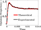
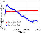
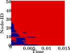
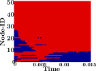
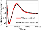
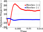
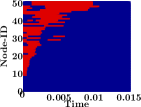
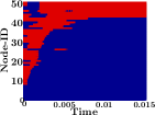
Figure 1: Opinion dynamics on two 50-node networks G1subscript𝐺1G_{1} (top) and G2subscript𝐺2G_{2} (bottom) for Poisson (P) and Hawkes (H) message intensities. The first column visualizes the two networks and opinion of each node at t=0𝑡0t=0 (positive/negative opinions in red/blue). The second column shows the temporal evolution of the theoretical and empirical average opinion for Poisson intensities. The third column shows the temporal evolution of the empirical average opinion for Hawkes intensities, where we compute the average separately for positive (++) and negative (-) opinions in the steady state. The fourth and fifth columns shows the polarity of average opinion per user over time.

3.2 Simulation based forecasting

Given the efficient simulation procedure described in Section 2.2, we can readily derive a general simulation based formula for opinion forecasting:

𝔼t\t0[𝒙(t)|t0]𝒙^(t)=1nl=1n𝒙l(t),subscript𝔼\subscript𝑡subscriptsubscript𝑡0delimited-[]conditionalsuperscript𝒙𝑡subscriptsubscript𝑡0superscript^𝒙𝑡1𝑛superscriptsubscript𝑙1𝑛superscriptsubscript𝒙𝑙𝑡\mathbb{E}_{\mathcal{H}_{t}\backslash\mathcal{H}_{t_{0}}}[\bm{x}^{*}(t)|\mathcal{H}_{t_{0}}]\approx\hat{\bm{x}}^{*}(t)=\frac{1}{n}\sum_{l=1}^{n}\bm{x}_{l}^{*}(t), (13)

where n𝑛n is the number of times that we simulate the opinion dynamics and 𝒙l(t)superscriptsubscript𝒙𝑙𝑡\bm{x}_{l}^{*}(t) gathers the users’ opinion at time t𝑡t for the l𝑙l-th simulation. Moreover, we have the following theoretical guarantee (proven in Appendix G):

Theorem 6.

Simulate the opinion dynamics up to time t>t0𝑡subscript𝑡0t>t_{0} the following number of times:

n13ϵ2(6σmax2+4xmaxϵ)log(2/δ),𝑛13superscriptitalic-ϵ26subscriptsuperscript𝜎2max4subscript𝑥maxitalic-ϵ2𝛿n\geq\frac{1}{3\epsilon^{2}}(6\sigma^{2}_{\text{max}}+4x_{\text{max}}\epsilon)\log(2/\delta), (14)

where σmax2=maxu𝒢σt\t02(xu(t)|t0)subscriptsuperscript𝜎2maxsubscript𝑢𝒢superscriptsubscript𝜎\subscript𝑡subscriptsubscript𝑡02conditionalsuperscriptsubscript𝑥𝑢𝑡subscriptsubscript𝑡0\sigma^{2}_{\text{max}}=\max_{u\in\mathcal{G}}\sigma_{\mathcal{H}_{t}\backslash\mathcal{H}_{t_{0}}}^{2}(x_{u}^{*}(t)|\mathcal{H}_{t_{0}}) is the maximum variance of the users’ opinions, which we analyze in Appendix G, and xmax|xu(t)|,u𝒢formulae-sequencesubscript𝑥maxsubscript𝑥𝑢𝑡for-all𝑢𝒢x_{\text{max}}\geq|x_{u}(t)|,\forall u\in\mathcal{G} is an upper bound on the users’ (absolute) opinions. Then, for each user u𝒢𝑢𝒢u\in\mathcal{G}, the error between her true and estimated average opinion satisfies that |x^u(t)𝔼t\t0[xu(t)|t0]|ϵ|\hat{x}_{u}^{*}(t)-\mathbb{E}_{\mathcal{H}_{t}\backslash\mathcal{H}_{t_{0}}}[x_{u}^{*}(t)|\mathcal{H}_{t_{0}}]|\leq\epsilon with probability at least 1δ1𝛿1-\delta.

4 Experiments

4.1 Experiments on synthetic data

We first provide empirical evidence that our model is able to produce different types of opinion dynamics, which may or may not converge to a steady state of consensus or polarization. Then, we show that our model estimation and simulation algorithms as well as our predictive formulas scale to networks with millions of users and events. Appendix J contains an evaluation of the accuracy of our model parameter estimation method.

Different types of opinion dynamics. We first simulate our model on two different small networks using Poisson intensities, i.e., λu(t)=μusubscriptsuperscript𝜆𝑢𝑡subscript𝜇𝑢\lambda^{*}_{u}(t)=\mu_{u}, μuU(0,1)similar-tosubscript𝜇𝑢𝑈01\mu_{u}\sim U(0,1) ufor-all𝑢\forall u, and then simulate our model on the same networks while using Hackers intensities with bvuU(0,1)similar-tosubscript𝑏𝑣𝑢𝑈01b_{vu}\sim U(0,1) on 5% of the nodes, chosen at random, and the original Poisson intensities on the remaining nodes. Figure 1 summarizes the results, which show that (i) our model is able to produce opinion dynamics that converge to consensus (second column) and polarization (third column); (ii) the opinion forecasting formulas described in Section 3 closely match an simulation based estimation (second column); and, (iii) the evolution of the average opinion and whether opinions converge to a steady state of consensus or polarization depend on the functional form of message intensity555For these particular networks, Poisson intensities lead to consensus while Hake’s intensities lead to polarization, however, we did find other examples in which Poisson intensities lead to polarization and Hawkes intensities lead to consensus..

Scalability. Figure 2 shows that our model estimation and simulation algorithms, described in Sections 2.1 and 2.2, and our analytical predictive formulas, described in Section 3.1, scale to networks with millions of users and events. For example, our algorithm takes 202020 minutes to estimate the model parameters from 10 million events generated by one million nodes using a single machine with 24 cores and 64 GB RAM.

Refer to caption

(a) Estimation vs # nodes

Refer to caption

(b) Simulation vs # nodes

Refer to caption

(c) Forecast vs # nodes

Refer to caption

(d) Forecast vs T𝑇T
Figure 2: Panels (a) and (b) show running time of our estimation and simulation procedures against number of nodes, where the average number of events per node is 101010. Panels (c) and (d) show the running time needed to compute our analytical formulas against number of nodes and time horizon T=tt0𝑇𝑡subscript𝑡0T=t-t_{0}, where the number of nodes is 103superscript10310^{3}. In Panel (c), T=6𝑇6T=6 hours. For all panels, the average degree per node is 303030. The experiments are carried out in a single machine with 24 cores and 64 GB of main memory.

4.2 Experiments on real data

We use real data gathered from Twitter to show that our model can forecast users’ opinions more accurately than six state of the art methods [6, 7, 8, 14, 18, 25].

Experimental Setup. We experimented with five Twitter datasets about current real-world events (Politics, Movie, Fight, Bollywood and US), in which, for each recorded message i𝑖i, we compute its sentiment value misubscript𝑚𝑖m_{i} using a popular sentiment analysis toolbox, specially designed for Twitter [12]. Here, the sentiment takes values m(1,1)𝑚11m\in(-1,1) and we consider the sentiment polarity to be simply sign(m)sign𝑚\mathop{\mathrm{sign}}(m). Appendix K contains further details and statistics about these datasets.

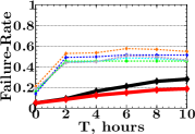
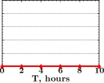
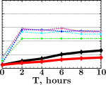
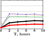
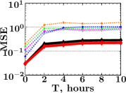
Opinion forecasting. We first evaluate the performance of our model at predicting sentiment (expressed opinion) at a message level. To do so, for each dataset, we first estimate the parameters of our model, SLANT, using messages from a training set containing the (chronologically) first 90% of the messages. Here, we set the decay parameters of the exponential triggering kernels κ(t)𝜅𝑡\kappa(t) and g(t)𝑔𝑡g(t) by cross-validation. Then, we evaluate the predictive performance of our opinion forecasting formulas using the last 10% of the messages666Here, we do not distinguish between analytical and sampling based forecasting since, in practice, they closely match each other.. More specifically, we predict the sentiment value m𝑚m for each message posted by user u𝑢u in the test set given the history up to T𝑇T hours before the time of the message as m^=Et\tT[xu(t)|tT]^𝑚subscript𝐸\subscript𝑡subscript𝑡𝑇delimited-[]conditionalsubscriptsuperscript𝑥𝑢𝑡subscript𝑡𝑇\hat{m}=E_{\mathcal{H}_{t}\backslash\mathcal{H}_{t-T}}[x^{*}_{u}(t)|\mathcal{H}_{t-T}]. We compare the performance of our model with the asynchronous linear model (AsLM) [7], DeGroot’s model [8], the voter model [25], the biased voter model [6], the flocking model [14], and the sentiment prediction method based on collaborative filtering by Kim et al. [18], in terms of: (i) the mean squared error between the true (m𝑚m) and the estimated (m^^𝑚\hat{m}) sentiment value for all messages in the held-out set, i.e., 𝔼[(mm^)2]𝔼delimited-[]superscript𝑚^𝑚2\mathbb{E}[(m-\hat{m})^{2}], and (ii) the failure rate, defined as the probability that the true and the estimated polarity do not coincide, i.e., (sign(m)sign(m^))sign𝑚sign^𝑚\mathbb{P}(\mathop{\mathrm{sign}}(m)\neq\mathop{\mathrm{sign}}(\hat{m})). For the baselines algorithms, which work in discrete time, we simulate NTsubscript𝑁𝑇N_{T} rounds in (tT,t)𝑡𝑇𝑡(t-T,t), where NTsubscript𝑁𝑇N_{T} is the number of posts in time T𝑇T. Figure 3 summarizes the results, which show that: (i) our opinion forecasting formulas consistently outperform others both in terms of MSE (often by an order of magnitude) and failure rate;777The failure rate is very close to zero for those datasets in which most users post messages with the same polarity. (ii) its forecasting performance degrades gracefully with respect to T𝑇T, in contrast, competing methods often fail catastrophically; and, (iii) it achieves an additional mileage by using Hawkes processes instead of Poisson processes. To some extent, we believe SLANT’s superior performance is due to its ability to leverage historical data to learn its model parameters and then simulate realistic temporal patterns.

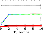
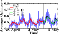
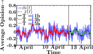
Finally, we look at the forecasting results at a network level and show that our forecasting formulas can also predict the evolution of opinions macroscopically (in terms of the average opinion across users). Figure 4 summarizes the results for two real world datasets, which show that the forecasted opinions become less accurate as the time T𝑇T becomes larger, since the average is computed on longer time periods. As expected, our model is more accurate when the message intensities are modeled using multivariate Hawkes. We found qualitatively similar results for the remaining datasets.

Refer to caption
Refer to caption
(a)
Refer to caption
(b)
Refer to caption
(c)
Refer to caption
(d)
Refer to caption
(e)
Refer to caption
(b) Politics
Refer to caption
(c) Movie
Refer to caption
(d) Fight
Refer to caption
(e) Bollywood
Refer to caption
(f) US
Figure 3: Sentiment prediction performance using a 101010% held-out set for each real-world dataset. Performance is measured in terms of mean squared error (MSE) on the sentiment value, 𝔼[(mm^)2]𝔼delimited-[]superscript𝑚^𝑚2\mathbb{E}[(m-\hat{m})^{2}], and failure rate on the sentiment polarity, (sign(m)sign(m^))sign𝑚sign^𝑚\mathbb{P}(\mathop{\mathrm{sign}}(m)\neq\mathop{\mathrm{sign}}(\hat{m})). For each message in the held-out set, we predict the sentiment value m𝑚m given the history up to T𝑇T hours before the time of the message, for different values of T𝑇T. Nowcasting corresponds to T=0𝑇0T=0 and forecasting to T>0𝑇0T>0. The sentiment value m(1,1)𝑚11m\in(-1,1) and the sentiment polarity sign(m){1,1}sign𝑚11\mathop{\mathrm{sign}}{(m)}\in\{-1,1\}.

5 Conclusions

Refer to caption
(a) Tw: Movie (Hawkes)
Refer to caption
(b) Tw: Movie (Poisson)
Refer to caption
(c) Tw: US (Hawkes)
Refer to caption
(d) Tw: US (Poisson)
Figure 4: Macroscopic sentiment prediction given by our model for two real-world datasets. The panels show the observed sentiment m¯(t)¯𝑚𝑡\bar{m}(t) (in blue, running average), inferred opinion x¯(t)¯𝑥𝑡\bar{x}(t) on the training set (in red), and forecasted opinion 𝔼t\tT[xu(t)|tT]subscript𝔼\subscript𝑡subscript𝑡𝑇delimited-[]conditionalsubscript𝑥𝑢𝑡subscript𝑡𝑇\mathbb{E}_{\mathcal{H}_{t}\backslash\mathcal{H}_{t-T}}[x_{u}(t)|\mathcal{H}_{t-T}] for T=1𝑇1T=1, 333, and 555 hours on the test set (in black, green and gray, respectively), where the symbol ¯¯absent\,\bar{}\, denotes average across users.

We proposed a modeling framework of opinion dynamics, whose key innovation is modeling users’ latent opinions as continuous-time stochastic processes driven by a set of marked jump stochastic differential equations (SDEs) [13]. Such construction allows each user’s latent opinion to be modulated over time by the opinions asynchronously expressed by her neighbors as sentiment messages. We then exploited a key property of our model, the Markov property, to design efficient parameter estimation and simulation algorithms, which scale to networks with millions of nodes. Moreover, we derived a set of novel predictive formulas for efficient and accurate opinion forecasting and identified conditions under which opinions converge to a steady state of consensus or polarization. Finally, we experimented with real data gathered from Twitter and showed that our framework achieves more accurate opinion forecasting than state-of-the-arts.

Our model opens up many interesting venues for future work. For example, in Eq. 4, our model assumes a linear dependence between users’ opinions, however, in some scenarios, this may be a coarse approximation. A natural follow-up to improve the opinion forecasting accuracy would be considering nonlinear dependences between opinions. It would be interesting to augment our model to jointly consider correlations between different topics. One could leverage our modeling framework to design opinion shaping algorithms based on stochastic optimal control [13, 24]. Finally, one of the key modeling ideas is realizing that users’ expressed opinions (be it in the form of thumbs up/down or text sentiment) can be viewed as noisy discrete samples of the users’ latent opinion localized in time. It would be very interesting to generalize this idea to any type of event data and derive sampling theorems and conditions under which an underlying general continuous signal of interest (be it user’s opinion, expertise, or wealth) can be recovered from event data with provable guarantees.

References

  • [1] O. Aalen, Ø. Borgan, and H. Gjessing. Survival and event history analysis: a process point of view. Springer Verlag, 2008.
  • [2] A. H. Al-Mohy and N. J. Higham. Computing the action of the matrix exponential, with an application to exponential integrators. SIAM journal on scientific computing, 33(2):488–511, 2011.
  • [3] R. Axelrod. The dissemination of culture a model with local convergence and global polarization. Journal of conflict resolution, 41(2):203–226, 1997.
  • [4] E. G. Birgin, J. M. Martínez, and M. Raydan. Nonmonotone spectral projected gradient methods on convex sets. SIAM Journal on Optimization, 10(4), 2000.
  • [5] P. Clifford and A. Sudbury. A model for spatial conflict. Biometrika, 60(3):581–588, 1973.
  • [6] A. Das, S. Gollapudi, and K. Munagala. Modeling opinion dynamics in social networks. In WSDM, 2014.
  • [7] A. De, S. Bhattacharya, P. Bhattacharya, N. Ganguly, and S. Chakrabarti. Learning a linear influence model from transient opinion dynamics. In CIKM, 2014.
  • [8] M. H. DeGroot. Reaching a consensus. Journal of the American Statistical Association, 69(345), 1974.
  • [9] M. Farajtabar, N. Du, M. Gomez-Rodriguez, I. Valera, L. Song, and H. Zha. Shaping social activity by incentivizing users. In NIPS, 2014.
  • [10] M. Farajtabar, Y. Wang, M. Gomez-Rodriguez, S. Li, H. Zha, and L. Song. Coevolve: A joint point process model for information diffusion and network co-evolution. In NIPS, 2015.
  • [11] M. Gomez-Rodriguez, D. Balduzzi, and B. Schölkopf. Uncovering the Temporal Dynamics of Diffusion Networks. In ICML, 2011.
  • [12] A. Hannak, E. Anderson, L. F. Barrett, S. Lehmann, A. Mislove, and M. Riedewald. Tweetin’in the rain: Exploring societal-scale effects of weather on mood. In ICWSM, 2012.
  • [13] F. B. Hanson. Applied Stochastic Processes and Control for Jump-Diffusions. SIAM, 2007.
  • [14] R. Hegselmann and U. Krause. Opinion dynamics and bounded confidence models, analysis, and simulation. Journal of Artificial Societies and Social Simulation, 5(3), 2002.
  • [15] D. Hinrichsen, A. Ilchmann, and A. Pritchard. Robustness of stability of time-varying linear systems. Journal of Differential Equations, 82(2):219 – 250, 1989.
  • [16] P. Holme and M. E. Newman. Nonequilibrium phase transition in the coevolution of networks and opinions. Physical Review E, 74(5):056108, 2006.
  • [17] T. Karppi and K. Crawford. Social media, financial algorithms and the hack crash. TC&S, 2015.
  • [18] J. Kim, J.-B. Yoo, H. Lim, H. Qiu, Z. Kozareva, and A. Galstyan. Sentiment prediction using collaborative filtering. In ICWSM, 2013.
  • [19] J. Leskovec, D. Chakrabarti, J. M. Kleinberg, C. Faloutsos, and Z. Ghahramani. Kronecker graphs: An approach to modeling networks. JMLR, 2010.
  • [20] B. Pang and L. Lee. Opinion mining and sentiment analysis. F&T in information retrieval, 2(1-2), 2008.
  • [21] B. H. Raven. The bases of power: Origins and recent developments. Journal of social issues, 49(4), 1993.
  • [22] Y. Saad and M. H. Schultz. Gmres: A generalized minimal residual algorithm for solving nonsymmetric linear systems. SIAM Journal on scientific and statistical computing, 7(3):856–869, 1986.
  • [23] I. Valera and M. Gomez-Rodriguez. Modeling adoption and usage of competing products. In Proceedings of the 2015 IEEE International Conference on Data Mining, 2015.
  • [24] Y. Wang, E. Theodorou, A. Verma, and L. Song. Steering opinion dynamics in information diffusion networks. arXiv preprint arXiv:1603.09021, 2016.
  • [25] M. E. Yildiz, R. Pagliari, A. Ozdaglar, and A. Scaglione. Voting models in random networks. In Information Theory and Applications Workshop, pages 1–7, 2010.

Appendix A Proof of Proposition 1

Given 𝒙(t):=[𝒙1(t),,𝒙|𝒱|(t)]Tassignsuperscript𝒙𝑡superscriptsubscript𝒙1𝑡subscript𝒙𝒱𝑡𝑇\bm{x}^{*}(t):=[\bm{x}_{1}(t),...,\bm{x}_{|\mathcal{V}|}(t)]^{T} and 𝝀(t):=[𝝀1(t),,𝝀|𝒱|(t)]Tassignsuperscript𝝀𝑡superscriptsubscript𝝀1𝑡subscript𝝀𝒱𝑡𝑇\boldsymbol{\lambda}^{*}(t):=[\boldsymbol{\lambda}_{1}(t),...,\boldsymbol{\lambda}_{|\mathcal{V}|}(t)]^{T}, we can compactly rewrite Eqs. 3 and 4 for all users as:

𝒙(t)=𝜶+𝑨0tg(tθ)𝒎(t)𝑑𝑵(t)superscript𝒙𝑡𝜶𝑨superscriptsubscript0𝑡direct-product𝑔𝑡𝜃𝒎𝑡differential-d𝑵𝑡\displaystyle\bm{x}^{*}(t)=\boldsymbol{\alpha}+\bm{A}\int_{0}^{t}g(t-\theta)\bm{m}(t)\odot d\bm{N}(t) (15)

and

𝝀(t)=𝝁+𝑩0tκ(tθ)𝑑𝑵(t).superscript𝝀𝑡𝝁𝑩superscriptsubscript0𝑡direct-product𝜅𝑡𝜃differential-d𝑵𝑡\displaystyle\boldsymbol{\lambda}^{*}(t)=\boldsymbol{\mu}+\bm{B}\int_{0}^{t}\kappa(t-\theta)\odot d\bm{N}(t). (16)

Then, it easily follows that

d𝒙(t)=𝑨0tg(tθ)𝒎(t)𝑑𝑵(t)+g(0)𝑨𝒎(t)d𝑵(t),𝑑superscript𝒙𝑡𝑨superscriptsubscript0𝑡direct-productsuperscript𝑔𝑡𝜃𝒎𝑡differential-d𝑵𝑡direct-product𝑔0𝑨𝒎𝑡𝑑𝑵𝑡\displaystyle d\bm{x}^{*}(t)=\bm{A}\int_{0}^{t}g^{\prime}(t-\theta)\bm{m}(t)\odot d\bm{N}(t)+g(0)\bm{A}\bm{m}(t)\odot d\bm{N}(t), (17)

where g(t)=eωt𝑔𝑡superscript𝑒𝜔𝑡g(t)=e^{-\omega t} and g(tθ)=ωg(tθ)superscript𝑔𝑡𝜃𝜔𝑔𝑡𝜃g^{\prime}(t-\theta)=-\omega g(t-\theta). And, we can rewrite the above expression as

d𝒙(t)=ω(𝜶𝐱(t))dt+𝐀(𝐦(t)d𝑵(t)).𝑑superscript𝒙𝑡𝜔𝜶superscript𝐱𝑡𝑑𝑡𝐀direct-product𝐦𝑡𝑑𝑵𝑡\displaystyle d\bm{x}^{*}(t)=\omega(\boldsymbol{\alpha}-\mathbf{x}^{*}(t))dt+\mathbf{A}(\mathbf{m}(t)\odot d\bm{N}(t)). (18)

Similarly, we can show that

d𝝀(t)𝑑superscript𝝀𝑡\displaystyle d\boldsymbol{\lambda}^{*}(t) =ν(𝝁𝝀(t))dt+𝐁d𝑵(t).absent𝜈𝝁superscript𝝀𝑡𝑑𝑡𝐁𝑑𝑵𝑡\displaystyle=\nu(\boldsymbol{\mu}-\boldsymbol{\lambda}^{*}(t))dt+\mathbf{B}\,d\bm{N}(t).

Appendix B Auxiliary theoretical results

The proofs of Theorems 2 and 5 rely on the following auxiliary Lemma.

Lemma 7.

The expected opinion 𝔼t\t0[𝐱(t)|t0]subscript𝔼\subscript𝑡subscriptsubscript𝑡0delimited-[]conditionalsuperscript𝐱𝑡subscriptsubscript𝑡0\mathbb{E}_{\mathcal{H}_{t}\backslash\mathcal{H}_{t_{0}}}[\bm{x}^{*}(t)|\mathcal{H}_{t_{0}}] in the model of opinion dynamics defined by Eqs. 4 and 3 with exponential triggering kernels with parameters ω𝜔\omega and ν𝜈\nu satisfies the following differential equation:

d𝔼t\t0[𝒙(t)|t0]dt=𝑨𝔼t\t0[𝒙(t)𝝀(t)|t0]ω𝔼t\t0[𝒙(t)|t0]+ω𝜶,𝑑subscript𝔼\subscript𝑡subscriptsubscript𝑡0delimited-[]conditionalsuperscript𝒙𝑡subscriptsubscript𝑡0𝑑𝑡𝑨subscript𝔼\subscript𝑡subscriptsubscript𝑡0delimited-[]conditionaldirect-productsuperscript𝒙𝑡superscript𝝀𝑡subscriptsubscript𝑡0𝜔subscript𝔼\subscript𝑡subscriptsubscript𝑡0delimited-[]conditionalsuperscript𝒙𝑡subscriptsubscript𝑡0𝜔𝜶\frac{d\mathbb{E}_{\mathcal{H}_{t}\backslash\mathcal{H}_{t_{0}}}[\bm{x}^{*}(t)|\mathcal{H}_{t_{0}}]}{dt}=\bm{A}\mathbb{E}_{\mathcal{H}_{t}\backslash\mathcal{H}_{t_{0}}}[\bm{x}^{*}(t)\odot\boldsymbol{\lambda}^{*}(t)|\mathcal{H}_{t_{0}}]-\omega\mathbb{E}_{\mathcal{H}_{t}\backslash\mathcal{H}_{t_{0}}}[\bm{x}^{*}(t)|\mathcal{H}_{t_{0}}]+\omega\boldsymbol{\alpha}, (19)

where 𝐀=(avu)v,u𝒢𝐀subscriptsubscript𝑎𝑣𝑢𝑣𝑢𝒢\bm{A}=(a_{vu})_{v,u\in\mathcal{G}} and the sign direct-product\odot denotes pointwise product.

Using that 𝔼[mv(θ)|xv(θ)]=xv(θ)𝔼delimited-[]conditionalsubscript𝑚𝑣𝜃subscriptsuperscript𝑥𝑣𝜃subscriptsuperscript𝑥𝑣𝜃\mathbb{E}[m_{v}(\theta)|x^{*}_{v}(\theta)]=x^{*}_{v}(\theta), we can compute the average opinion of user u𝑢u across all possible histories from Eq. 4 as

𝔼t\t0[xu(t)|t0]=αu+v𝒩(u)auv0tg(tθ)𝔼t\t0[mv(θ)dNv(θ)|t0]subscript𝔼\subscript𝑡subscriptsubscript𝑡0delimited-[]conditionalsubscriptsuperscript𝑥𝑢𝑡subscriptsubscript𝑡0subscript𝛼𝑢subscript𝑣𝒩𝑢subscript𝑎𝑢𝑣superscriptsubscript0𝑡𝑔𝑡𝜃subscript𝔼\subscript𝑡subscriptsubscript𝑡0delimited-[]conditionalsubscript𝑚𝑣𝜃𝑑subscript𝑁𝑣𝜃subscriptsubscript𝑡0\displaystyle\mathbb{E}_{\mathcal{H}_{t}\backslash\mathcal{H}_{t_{0}}}[x^{*}_{u}(t)|\mathcal{H}_{t_{0}}]=\alpha_{u}+\sum_{v\in\mathcal{N}(u)}a_{uv}\int_{0}^{t}g(t-\theta)\mathbb{E}_{\mathcal{H}_{t}\backslash\mathcal{H}_{t_{0}}}[m_{v}(\theta)dN_{v}(\theta)|\mathcal{H}_{t_{0}}]
=αu+v𝒩(u)auvtiv(t0)g(tti)mv(ti)+v𝒩(u)auvt0tg(tθ)𝔼(θ)\t0[xv(θ)λv(θ)|t0]𝑑θ,absentsubscript𝛼𝑢subscript𝑣𝒩𝑢subscript𝑎𝑢𝑣subscriptsubscript𝑡𝑖subscript𝑣subscript𝑡0𝑔𝑡subscript𝑡𝑖subscript𝑚𝑣subscript𝑡𝑖subscript𝑣𝒩𝑢subscript𝑎𝑢𝑣superscriptsubscriptsubscript𝑡0𝑡𝑔𝑡𝜃subscript𝔼\𝜃subscriptsubscript𝑡0delimited-[]conditionalsubscriptsuperscript𝑥𝑣𝜃subscriptsuperscript𝜆𝑣𝜃subscriptsubscript𝑡0differential-d𝜃\displaystyle=\alpha_{u}+\sum_{v\in\mathcal{N}(u)}a_{uv}\sum_{t_{i}\in\mathcal{H}_{v}(t_{0})}g(t-t_{i})m_{v}(t_{i})+\sum_{v\in\mathcal{N}(u)}a_{uv}\int_{t_{0}}^{t}g(t-\theta)\mathbb{E}_{\mathcal{H}(\theta)\backslash\mathcal{H}_{t_{0}}}\big{[}x^{*}_{v}(\theta)\lambda^{*}_{v}(\theta)|\mathcal{H}_{t_{0}}\big{]}d\theta,

and we can write the expectation of the opinion for all users in vectorial form as

𝔼t\t0[𝒙(t)]=𝒗(t)+𝑨0tg(tθ)𝔼(θ)\t0[𝒙(θ)𝝀(θ)]𝑑θ,subscript𝔼\subscript𝑡subscriptsubscript𝑡0delimited-[]superscript𝒙𝑡𝒗𝑡𝑨superscriptsubscript0𝑡𝑔𝑡𝜃subscript𝔼\𝜃subscriptsubscript𝑡0delimited-[]direct-productsuperscript𝒙𝜃superscript𝝀𝜃differential-d𝜃\mathbb{E}_{\mathcal{H}_{t}\backslash\mathcal{H}_{t_{0}}}[\bm{x}^{*}(t)]=\bm{v}(t)+\bm{A}\int_{0}^{t}g(t-\theta)\mathbb{E}_{\mathcal{H}(\theta)\backslash\mathcal{H}_{t_{0}}}[\bm{x}^{*}(\theta)\odot\boldsymbol{\lambda}^{*}(\theta)]d\theta, (20)

where the direct-product\odot denotes pointwise product and

(𝒗(t))u=αu+v𝒩(u)auvtiv(t0)g(tti)mv(ti).subscript𝒗𝑡𝑢subscript𝛼𝑢subscript𝑣𝒩𝑢subscript𝑎𝑢𝑣subscriptsubscript𝑡𝑖subscript𝑣subscript𝑡0𝑔𝑡subscript𝑡𝑖subscript𝑚𝑣subscript𝑡𝑖(\bm{v}(t))_{u}=\alpha_{u}+\sum_{v\in\mathcal{N}(u)}a_{uv}\sum_{t_{i}\in\mathcal{H}_{v}(t_{0})}g(t-t_{i})m_{v}(t_{i}).

Since g(t)=eωt𝑔𝑡superscript𝑒𝜔𝑡g(t)=e^{-\omega t}, one may observe that ω𝒗(t)+𝒗˙(t)=ωα𝜔𝒗𝑡˙𝒗𝑡𝜔𝛼\omega\bm{v}(t)+\dot{\bm{v}}(t)=\omega\alpha. Then, by differentiating Eq. 20, we obtain

d𝔼t\t0[𝒙(t)|t0]dt=𝑨𝔼t\t0[𝒙(t)𝝀(t)|t0]ω𝔼t\t0[𝒙(t)|t0]+ω𝜶,𝑑subscript𝔼\subscript𝑡subscriptsubscript𝑡0delimited-[]conditionalsuperscript𝒙𝑡subscriptsubscript𝑡0𝑑𝑡𝑨subscript𝔼\subscript𝑡subscriptsubscript𝑡0delimited-[]conditionaldirect-productsuperscript𝒙𝑡superscript𝝀𝑡subscriptsubscript𝑡0𝜔subscript𝔼\subscript𝑡subscriptsubscript𝑡0delimited-[]conditionalsuperscript𝒙𝑡subscriptsubscript𝑡0𝜔𝜶\frac{d\mathbb{E}_{\mathcal{H}_{t}\backslash\mathcal{H}_{t_{0}}}[\bm{x}^{*}(t)|\mathcal{H}_{t_{0}}]}{dt}=\bm{A}\mathbb{E}_{\mathcal{H}_{t}\backslash\mathcal{H}_{t_{0}}}[\bm{x}^{*}(t)\odot\boldsymbol{\lambda}^{*}(t)|\mathcal{H}_{t_{0}}]-\omega\mathbb{E}_{\mathcal{H}_{t}\backslash\mathcal{H}_{t_{0}}}[\bm{x}^{*}(t)|\mathcal{H}_{t_{0}}]+\omega\boldsymbol{\alpha}, (21)

Appendix C Proof of Theorem 2

Using Lemma 7 and λu(t)=μusubscriptsuperscript𝜆𝑢𝑡subscript𝜇𝑢\lambda^{*}_{u}(t)=\mu_{u}, we obtain

d𝔼t[𝒙(t)]dt=[ωI+𝑨𝚲1]𝔼t[𝒙(t)]+ω𝜶,𝑑subscript𝔼subscript𝑡delimited-[]superscript𝒙𝑡𝑑𝑡delimited-[]𝜔𝐼𝑨subscript𝚲1subscript𝔼subscript𝑡delimited-[]superscript𝒙𝑡𝜔𝜶\frac{d\mathbb{E}_{\mathcal{H}_{t}}[\bm{x}^{*}(t)]}{dt}=[-\omega I+\bm{A}\boldsymbol{\Lambda}_{1}]\mathbb{E}_{\mathcal{H}_{t}}[\bm{x}^{*}(t)]+\omega\boldsymbol{\alpha}, (22)

where 𝚲1=diag[𝝁]subscript𝚲1diagdelimited-[]𝝁\boldsymbol{\Lambda}_{1}=\mathop{\mathrm{diag}}[\boldsymbol{\mu}]. Then, we apply the Laplace transform to the expression above and obtain

𝒙^(s)=[sI+ωIA𝚲1]1𝒙(t0)+ωs[sI+ωIA𝚲1]1𝜶,^𝒙𝑠superscriptdelimited-[]𝑠𝐼𝜔𝐼𝐴subscript𝚲11𝒙subscript𝑡0𝜔𝑠superscriptdelimited-[]𝑠𝐼𝜔𝐼𝐴subscript𝚲11𝜶\hat{\bm{x}}(s)=[sI+\omega I-A\boldsymbol{\Lambda}_{1}]^{-1}\bm{x}(t_{0})+\frac{\omega}{s}[sI+\omega I-A\boldsymbol{\Lambda}_{1}]^{-1}\bm{\alpha},

where we leverage the fact that, conditioning the prior history, the opinion is non-random, i.e., 𝔼t0\t0[𝒙(t0)|t0]=𝒙(t0)subscript𝔼\subscriptsubscript𝑡0subscriptsubscriptsuperscript𝑡0delimited-[]conditional𝒙subscript𝑡0subscriptsubscriptsuperscript𝑡0𝒙subscript𝑡0\mathbb{E}_{\mathcal{H}_{t_{0}}\backslash\mathcal{H}_{t^{-}_{0}}}{[\bm{x}(t_{0})|\mathcal{H}_{t^{-}_{0}}]}=\bm{x}(t_{0}). Finally, applying the inverse Laplace transform, we obtain the average opinion 𝔼t\t0[𝒙(t)|t0]subscript𝔼\subscript𝑡subscriptsubscript𝑡0delimited-[]conditionalsuperscript𝒙𝑡subscriptsubscript𝑡0\mathbb{E}_{\mathcal{H}_{t}\backslash\mathcal{H}_{t_{0}}}[\bm{x}^{*}(t)|\mathcal{H}_{t_{0}}] in time domain as

𝔼t\t0[𝒙(t)|t0]subscript𝔼\subscript𝑡subscriptsubscript𝑡0delimited-[]conditionalsuperscript𝒙𝑡subscriptsubscript𝑡0\displaystyle\mathbb{E}_{\mathcal{H}_{t}\backslash\mathcal{H}_{t_{0}}}[\bm{x}^{*}(t)|\mathcal{H}_{t_{0}}] =e(𝑨𝚲1ωI)(tt0)𝒙(t0)+ω(𝑨𝚲1ωI)1(e(𝑨𝚲1ω𝑰)(tt0)𝑰)]𝜶.\displaystyle=e^{(\bm{A}\boldsymbol{\Lambda}_{1}-\omega I)(t-t_{0})}\bm{x}(t_{0})+\omega(\bm{A}\boldsymbol{\Lambda}_{1}-\omega I)^{-1}\left(e^{(\bm{A}\boldsymbol{\Lambda}_{1}-\omega\bm{I})(t-t_{0})}-\bm{I}\right)\Big{]}\bm{\alpha}.

Appendix D Proof of Theorem 3

Theorem 2 states that the average users’ opinion 𝔼t[𝒙(t)]subscript𝔼subscript𝑡delimited-[]superscript𝒙𝑡\mathbb{E}_{\mathcal{H}_{t}}[\bm{x}^{*}(t)] in time domain is given by

𝔼t\t0[𝒙(t)|t0]subscript𝔼\subscript𝑡subscriptsubscript𝑡0delimited-[]conditionalsuperscript𝒙𝑡subscriptsubscript𝑡0\displaystyle\mathbb{E}_{\mathcal{H}_{t}\backslash\mathcal{H}_{t_{0}}}[\bm{x}^{*}(t)|\mathcal{H}_{t_{0}}] =e(𝑨𝚲1ωI)(tt0)𝒙(t0)+ω(𝑨𝚲1ωI)1(e(𝑨𝚲1ω𝑰)(tt0)𝑰)]𝜶.\displaystyle=e^{(\bm{A}\boldsymbol{\Lambda}_{1}-\omega I)(t-t_{0})}\bm{x}(t_{0})+\omega(\bm{A}\boldsymbol{\Lambda}_{1}-\omega I)^{-1}\left(e^{(\bm{A}\boldsymbol{\Lambda}_{1}-\omega\bm{I})(t-t_{0})}-\bm{I}\right)\Big{]}\bm{\alpha}.

If Re[ξ(𝑨𝚲1)]<ω𝑅𝑒delimited-[]𝜉𝑨subscript𝚲1𝜔Re[\xi(\bm{A}\boldsymbol{\Lambda}_{1})]<\omega, where ξ(𝑿)𝜉𝑿\xi(\bm{X}) denote the eigenvalues of matrix 𝑿𝑿\bm{X}, it easily follows that

limt𝔼t[𝒙(t)]=(I𝑨𝚲1w)1𝜶.subscript𝑡subscript𝔼subscript𝑡delimited-[]superscript𝒙𝑡superscript𝐼𝑨subscript𝚲1𝑤1𝜶\lim_{t\to\infty}\mathbb{E}_{\mathcal{H}_{t}}[\bm{x}^{*}(t)]=\left(I-\frac{\bm{A}\boldsymbol{\Lambda}_{1}}{w}\right)^{-1}\bm{\alpha}. (23)

Appendix E Proof of Theorem 4

Assume bvu=0subscript𝑏𝑣𝑢0b_{vu}=0 for all v,u𝒢,vuformulae-sequence𝑣𝑢𝒢𝑣𝑢v,u\in\mathcal{G},v\neq u. Then, λv(t)subscriptsuperscript𝜆𝑣𝑡\lambda^{*}_{v}(t) only depends on user v𝑣v’s history and, since xv(t)subscriptsuperscript𝑥𝑣𝑡x^{*}_{v}(t) only depends on the history of the user v𝑣v’s neighbors 𝒩(v)𝒩𝑣\mathcal{N}(v), we can write

𝔼t\t0[𝒙(t)𝝀(t)|t0]=𝔼t\t0[𝒙(t)|t0]𝔼t\t0[𝝀(t)],subscript𝔼\subscript𝑡subscriptsubscript𝑡0delimited-[]conditionaldirect-productsuperscript𝒙𝑡superscript𝝀𝑡subscriptsubscript𝑡0direct-productsubscript𝔼\subscript𝑡subscriptsubscript𝑡0delimited-[]conditionalsuperscript𝒙𝑡subscriptsubscript𝑡0subscript𝔼\subscript𝑡subscriptsubscript𝑡0delimited-[]superscript𝝀𝑡\mathbb{E}_{\mathcal{H}_{t}\backslash\mathcal{H}_{t_{0}}}[\bm{x}^{*}(t)\odot\boldsymbol{\lambda}^{*}(t)|\mathcal{H}_{t_{0}}]=\mathbb{E}_{\mathcal{H}_{t}\backslash\mathcal{H}_{t_{0}}}\big{[}\bm{x}^{*}(t)|\mathcal{H}_{t_{0}}\big{]}\odot\mathbb{E}_{\mathcal{H}_{t}\backslash\mathcal{H}_{t_{0}}}\big{[}\boldsymbol{\lambda}^{*}(t)\big{]},

and rewrite Eq. 21 as

d𝔼t\t0[𝒙(t)|t0]dt=𝑑subscript𝔼\subscript𝑡subscriptsubscript𝑡0delimited-[]conditionalsuperscript𝒙𝑡subscriptsubscript𝑡0𝑑𝑡absent\displaystyle\frac{d\mathbb{E}_{\mathcal{H}_{t}\backslash\mathcal{H}_{t_{0}}}[\bm{x}^{*}(t)|\mathcal{H}_{t_{0}}]}{dt}= (24)
𝑨(𝔼t\t0[𝒙(t)|t0]𝔼t\t0[𝝀(t)|t0])ω𝔼t\t0[𝒙(t)|t0]+ω𝜶.𝑨direct-productsubscript𝔼\subscript𝑡subscriptsubscript𝑡0delimited-[]conditionalsuperscript𝒙𝑡subscriptsubscript𝑡0subscript𝔼\subscript𝑡subscriptsubscript𝑡0delimited-[]conditionalsuperscript𝝀𝑡subscriptsubscript𝑡0𝜔subscript𝔼\subscript𝑡subscriptsubscript𝑡0delimited-[]conditionalsuperscript𝒙𝑡subscriptsubscript𝑡0𝜔𝜶\displaystyle\bm{A}(\mathbb{E}_{\mathcal{H}_{t}\backslash\mathcal{H}_{t_{0}}}[\bm{x}^{*}(t)|\mathcal{H}_{t_{0}}]\odot\mathbb{E}_{\mathcal{H}_{t}\backslash\mathcal{H}_{t_{0}}}[\boldsymbol{\lambda}^{*}(t)|\mathcal{H}_{t_{0}}])-\omega\mathbb{E}_{\mathcal{H}_{t}\backslash\mathcal{H}_{t_{0}}}[\bm{x}^{*}(t)|\mathcal{H}_{t_{0}}]+\omega\boldsymbol{\alpha}.

We can now compute 𝔼(θ)\t0[𝝀(θ)|t0]subscript𝔼\𝜃subscriptsubscript𝑡0delimited-[]conditionalsuperscript𝝀𝜃subscriptsubscript𝑡0\mathbb{E}_{\mathcal{H}(\theta)\backslash\mathcal{H}_{t_{0}}}[\boldsymbol{\lambda}^{*}(\theta)|\mathcal{H}_{t_{0}}] analytically as follows. From Eq. 3, we obtain

𝔼t\t0[𝝀(t)|t0]=𝜼(t)+t0t𝑩κ(tθ)𝔼θ\t0[𝝀(θ)]𝑑θ,subscript𝔼\subscript𝑡subscriptsubscript𝑡0delimited-[]conditionalsuperscript𝝀𝑡subscriptsubscript𝑡0𝜼𝑡superscriptsubscriptsubscript𝑡0𝑡𝑩𝜅𝑡𝜃subscript𝔼\subscript𝜃subscriptsubscript𝑡0delimited-[]superscript𝝀𝜃differential-d𝜃\mathbb{E}_{\mathcal{H}_{t}\backslash\mathcal{H}_{t_{0}}}\big{[}\boldsymbol{\lambda}^{*}(t)|\mathcal{H}_{t_{0}}\big{]}=\bm{\eta}(t)+\int_{t_{0}}^{t}\bm{B}\kappa(t-\theta)\mathbb{E}_{\mathcal{H}_{\theta}\backslash\mathcal{H}_{t_{0}}}\big{[}\boldsymbol{\lambda}^{*}(\theta)\big{]}d\theta, (25)

where κ(t)=eνt𝜅𝑡superscript𝑒𝜈𝑡\kappa(t)=e^{-\nu t}, [𝜼(t)]u𝒱=μu+v𝒩(u)buvtiv(t0)κ(tti)subscriptdelimited-[]𝜼𝑡𝑢𝒱subscript𝜇𝑢subscript𝑣𝒩𝑢subscript𝑏𝑢𝑣subscriptsubscript𝑡𝑖subscript𝑣subscript𝑡0𝜅𝑡subscript𝑡𝑖[\bm{\eta}(t)]_{u\in\mathcal{V}}=\mu_{u}+\sum_{v\in\mathcal{N}(u)}b_{uv}\sum_{t_{i}\in\mathcal{H}_{v}(t_{0})}\kappa(t-t_{i}) and 𝑩=(bvu)v,u𝒱𝑩subscriptsubscript𝑏𝑣𝑢𝑣𝑢𝒱\bm{B}=(b_{vu})_{v,u\in\mathcal{V}}, where bvu=0subscript𝑏𝑣𝑢0b_{vu}=0 for all vu𝑣𝑢v\neq u, by assumption. Differentiating with respect to t𝑡t, we get,

ddt𝔼t\t0[𝝀(t)|t0]𝑑𝑑𝑡subscript𝔼\subscript𝑡subscriptsubscript𝑡0delimited-[]conditionalsuperscript𝝀𝑡subscriptsubscript𝑡0\displaystyle\frac{d}{dt}{\mathbb{E}_{\mathcal{H}_{t}\backslash\mathcal{H}_{t_{0}}}\big{[}\boldsymbol{\lambda}^{*}(t)|\mathcal{H}_{t_{0}}\big{]}} =ν𝔼t\t0[𝝀(t)|t0]+𝑩𝔼t\t0[𝝀(t)|t0]+ν𝝁,absent𝜈subscript𝔼\subscript𝑡subscriptsubscript𝑡0delimited-[]conditionalsuperscript𝝀𝑡subscriptsubscript𝑡0𝑩subscript𝔼\subscript𝑡subscriptsubscript𝑡0delimited-[]conditionalsuperscript𝝀𝑡subscriptsubscript𝑡0𝜈𝝁\displaystyle=-\nu\mathbb{E}_{\mathcal{H}_{t}\backslash\mathcal{H}_{t_{0}}}\big{[}\boldsymbol{\lambda}^{*}(t)|\mathcal{H}_{t_{0}}\big{]}+\bm{B}\mathbb{E}_{\mathcal{H}_{t}\backslash\mathcal{H}_{t_{0}}}\big{[}\boldsymbol{\lambda}^{*}(t)|\mathcal{H}_{t_{0}}\big{]}+\nu\boldsymbol{\mu},

with initial condition 𝔼(t0+)\(t0)𝝀(t0)=𝜼(t0)subscript𝔼\subscriptsuperscript𝑡0subscript𝑡0superscript𝝀subscript𝑡0𝜼subscript𝑡0\mathbb{E}_{\mathcal{H}(t^{+}_{0})\backslash\mathcal{H}(t_{0})}\boldsymbol{\lambda}^{*}(t_{0})=\bm{\eta}(t_{0}). By taking the Laplace transform and then applying inverse Laplace transform,

𝔼t\t0[𝝀(t)|t0]=e(𝑩νI)(tt0)𝜼(t0)+ν(𝑩νI)1(e(𝑩ν𝑰)(tt0)𝑰)𝝁 tt0,subscript𝔼\subscript𝑡subscriptsubscript𝑡0delimited-[]conditionalsuperscript𝝀𝑡subscriptsubscript𝑡0superscript𝑒𝑩𝜈𝐼𝑡subscript𝑡0𝜼subscript𝑡0𝜈superscript𝑩𝜈𝐼1superscript𝑒𝑩𝜈𝑰𝑡subscript𝑡0𝑰𝝁 for-all𝑡subscript𝑡0\mathbb{E}_{\mathcal{H}_{t}\backslash\mathcal{H}_{t_{0}}}[\boldsymbol{\lambda}^{*}(t)|\mathcal{H}_{t_{0}}]=e^{(\bm{B}-\nu I)(t-t_{0})}\bm{\eta}(t_{0})+\nu(\bm{B}-\nu I)^{-1}\left(e^{(\bm{B}-\nu\bm{I})(t-t_{0})}-\bm{I}\right)\boldsymbol{\mu}\text{ }\forall t\geq t_{0}, (26)

where 𝜼(t0)=𝔼(t0+)\(t0)[𝝀(t0)]𝜼subscript𝑡0subscript𝔼\subscriptsuperscript𝑡0subscript𝑡0delimited-[]superscript𝝀subscript𝑡0\bm{\eta}(t_{0})=\mathbb{E}_{\mathcal{H}(t^{+}_{0})\backslash\mathcal{H}(t_{0})}[\boldsymbol{\lambda}^{*}(t_{0})]. Using Eqs. 24 and 26, as well as 𝔼t\t0[𝒙(t)]𝔼t\t0[𝝀(t)]=𝚲(t)𝔼t\t0[𝒙(t)]direct-productsubscript𝔼\subscript𝑡subscriptsubscript𝑡0delimited-[]superscript𝒙𝑡subscript𝔼\subscript𝑡subscriptsubscript𝑡0delimited-[]superscript𝝀𝑡𝚲𝑡subscript𝔼\subscript𝑡subscriptsubscript𝑡0delimited-[]superscript𝒙𝑡\mathbb{E}_{\mathcal{H}_{t}\backslash\mathcal{H}_{t_{0}}}[\bm{x}^{*}(t)]\odot\mathbb{E}_{\mathcal{H}_{t}\backslash\mathcal{H}_{t_{0}}}[\boldsymbol{\lambda}^{*}(t)]=\boldsymbol{\Lambda}(t)\mathbb{E}_{\mathcal{H}_{t}\backslash\mathcal{H}_{t_{0}}}[\bm{x}^{*}(t)], where 𝚲(t):=diag[𝔼t\t0[𝝀(t)]]assign𝚲𝑡diagdelimited-[]subscript𝔼\subscript𝑡subscriptsubscript𝑡0delimited-[]superscript𝝀𝑡\boldsymbol{\Lambda}(t):=\mathop{\mathrm{diag}}[\mathbb{E}_{\mathcal{H}_{t}\backslash\mathcal{H}_{t_{0}}}[\boldsymbol{\lambda}^{*}(t)]], we obtain

d𝔼t\t0[𝒙(t)]dt=[ωI+𝑨𝚲(t)]𝔼t\t0[𝒙(t)]+ω𝜶,𝑑subscript𝔼\subscript𝑡subscriptsubscript𝑡0delimited-[]superscript𝒙𝑡𝑑𝑡delimited-[]𝜔𝐼𝑨𝚲𝑡subscript𝔼\subscript𝑡subscriptsubscript𝑡0delimited-[]superscript𝒙𝑡𝜔𝜶\displaystyle\frac{d\mathbb{E}_{\mathcal{H}_{t}\backslash\mathcal{H}_{t_{0}}}[\bm{x}^{*}(t)]}{dt}=[-\omega I+\bm{A}\boldsymbol{\Lambda}(t)]\mathbb{E}_{\mathcal{H}_{t}\backslash\mathcal{H}_{t_{0}}}[\bm{x}^{*}(t)]+\omega\boldsymbol{\alpha},

with initial conditions (𝔼(t0+)\(t0)[𝒙(t0)])u𝒱=αu+v𝒩(u)auvtiv(t0)g(t0ti)mv(ti)subscriptsubscript𝔼\superscriptsubscript𝑡0subscript𝑡0delimited-[]superscript𝒙subscript𝑡0𝑢𝒱subscript𝛼𝑢subscript𝑣𝒩𝑢subscript𝑎𝑢𝑣subscriptsubscript𝑡𝑖subscript𝑣subscript𝑡0𝑔subscript𝑡0subscript𝑡𝑖subscript𝑚𝑣subscript𝑡𝑖(\mathbb{E}_{\mathcal{H}(t_{0}^{+})\backslash\mathcal{H}(t_{0})}[\bm{x}^{*}(t_{0})])_{u\in\mathcal{V}}=\alpha_{u}+\sum_{v\in\mathcal{N}(u)}a_{uv}\sum_{t_{i}\in\mathcal{H}_{v}(t_{0})}g(t_{0}-t_{i})m_{v}(t_{i}).

Appendix F Proof of Theorem 5

Theorem 4 states that the average users’ opinion 𝔼t[𝒙(t)]subscript𝔼subscript𝑡delimited-[]superscript𝒙𝑡\mathbb{E}_{\mathcal{H}_{t}}[\bm{x}^{*}(t)] in time domain is given by

d𝔼t\t0[𝒙(t)|t0]dt=[ωI+𝑨𝚲(t)]𝔼t\t0[𝒙(t)|t0]+ω𝜶.𝑑subscript𝔼\subscript𝑡subscriptsubscript𝑡0delimited-[]conditionalsuperscript𝒙𝑡subscriptsubscript𝑡0𝑑𝑡delimited-[]𝜔𝐼𝑨𝚲𝑡subscript𝔼\subscript𝑡subscriptsubscript𝑡0delimited-[]conditionalsuperscript𝒙𝑡subscriptsubscript𝑡0𝜔𝜶\frac{d\mathbb{E}_{\mathcal{H}_{t}\backslash\mathcal{H}_{t_{0}}}[\bm{x}^{*}(t)|\mathcal{H}_{t_{0}}]}{dt}=[-\omega I+\bm{A}\boldsymbol{\Lambda}(t)]\mathbb{E}_{\mathcal{H}_{t}\backslash\mathcal{H}_{t_{0}}}[\bm{x}^{*}(t)|\mathcal{H}_{t_{0}}]+\omega\boldsymbol{\alpha}. (27)

In such systems, solutions can be written as [15]

𝔼t\t0[𝒙(t)|t0]=Φ(t)α+ω0tΦ(s)𝜶𝑑s,subscript𝔼\subscript𝑡subscriptsubscript𝑡0delimited-[]conditionalsuperscript𝒙𝑡subscriptsubscript𝑡0Φ𝑡𝛼𝜔superscriptsubscript0𝑡Φ𝑠𝜶differential-d𝑠\mathbb{E}_{\mathcal{H}_{t}\backslash\mathcal{H}_{t_{0}}}[\bm{x}^{*}(t)|\mathcal{H}_{t_{0}}]=\Phi(t)\alpha+\omega\int_{0}^{t}\Phi(s)\boldsymbol{\alpha}ds, (28)

where the transition matrix Φ(t)Φ𝑡\Phi(t) defines as a solution of the matrix differential equation

Φ˙(t)=[ωI+𝑨𝚲(t)]Φ(t) with Φ(0)=I.˙Φ𝑡delimited-[]𝜔𝐼𝑨𝚲𝑡Φ𝑡 with Φ0𝐼\dot{\Phi}(t)=[-\omega I+\bm{A}\boldsymbol{\Lambda}(t)]\Phi(t)\text{ with }\Phi(0)=I.

If Φ(t)Φ𝑡\Phi(t) satisfies Φ(t)γectnormΦ𝑡𝛾superscript𝑒𝑐𝑡||\Phi(t)||\leq\gamma e^{-ct} t>0for-all𝑡0\forall t>0 for γ,c>0𝛾𝑐0\gamma,c>0 then the steady state solution to Eq. 28 is given by [15]

limt𝔼t\t0[𝒙(t)|t0]=(I𝑨𝚲2ω)1𝜶.subscript𝑡subscript𝔼\subscript𝑡subscriptsubscript𝑡0delimited-[]conditionalsuperscript𝒙𝑡subscriptsubscript𝑡0superscript𝐼𝑨subscript𝚲2𝜔1𝜶\displaystyle\lim_{t\to\infty}\mathbb{E}_{\mathcal{H}_{t}\backslash\mathcal{H}_{t_{0}}}[\bm{x}^{*}(t)|\mathcal{H}_{t_{0}}]=\left(I-\frac{\bm{A}\boldsymbol{\Lambda}_{2}}{\omega}\right)^{-1}\boldsymbol{\alpha}.

where 𝚲2=limt𝚲(t)=diag[I𝑩ν]1𝝁subscript𝚲2subscript𝑡𝚲𝑡diagsuperscriptdelimited-[]𝐼𝑩𝜈1𝝁\boldsymbol{\Lambda}_{2}=\lim_{t\to\infty}\boldsymbol{\Lambda}(t)=\mathop{\mathrm{diag}}\Big{[}I-\frac{\bm{B}}{\nu}\Big{]}^{-1}\boldsymbol{\mu}.

Appendix G Proof of Theorem 6

Let {𝒙l(t)}l=1nsuperscriptsubscriptsuperscriptsubscript𝒙𝑙𝑡𝑙1𝑛\{{\bm{x}}_{l}^{*}(t)\}_{l=1}^{n} be the simulated opinions for all users and define 𝒔(t)=1nl=1n𝒔l(t)𝒔𝑡1𝑛superscriptsubscript𝑙1𝑛subscript𝒔𝑙𝑡\bm{s}(t)=\frac{1}{n}\sum_{l=1}^{n}\bm{s}_{l}(t), where 𝒔l(t)=(𝒙^l(t)𝔼t\t0[𝒙(t)|t0])subscript𝒔𝑙𝑡superscriptsubscript^𝒙𝑙𝑡subscript𝔼\subscript𝑡subscriptsubscript𝑡0delimited-[]conditionalsuperscript𝒙𝑡subscriptsubscript𝑡0\bm{s}_{l}(t)=(\hat{\bm{x}}_{l}^{*}(t)-\mathbb{E}_{\mathcal{H}_{t}\backslash\mathcal{H}_{t_{0}}}[\bm{x}^{*}(t)|\mathcal{H}_{t_{0}}]). Clearly, for a given t𝑡t, all elements in 𝒔l(t)subscript𝒔𝑙𝑡\bm{s}_{l}(t) are i.i.d. random variables with zero mean and variance, and we can bound |su(t)|<2xmaxsubscript𝑠𝑢𝑡2subscript𝑥max|s_{u}(t)|<2x_{\text{max}}. Then, by Bernstein’s inequality, the following holds true,

(|su(t)|>ϵ)=(su(t)>ϵ)+(su(t)<ϵ)>2.exp(3nϵ26σt\t02(xu(t)|t0)+4xmaxϵ)formulae-sequencesubscript𝑠𝑢𝑡italic-ϵsubscript𝑠𝑢𝑡italic-ϵsubscript𝑠𝑢𝑡italic-ϵ2exp3𝑛superscriptitalic-ϵ26superscriptsubscript𝜎\subscript𝑡subscriptsubscript𝑡02conditionalsuperscriptsubscript𝑥𝑢𝑡subscriptsubscript𝑡04subscript𝑥maxitalic-ϵ\mathbb{P}(|s_{u}(t)|>\epsilon)=\mathbb{P}(s_{u}(t)>\epsilon)+\mathbb{P}(s_{u}(t)<-\epsilon)>2.\text{exp}{\Big{(}-\frac{3n\epsilon^{2}}{6\sigma_{\mathcal{H}_{t}\backslash\mathcal{H}_{t_{0}}}^{2}(x_{u}^{*}(t)|\mathcal{H}_{t_{0}})+4x_{\text{max}}\epsilon}\Big{)}}

Let σmax2(t)=maxu𝒢σt\t02(xu(t)|t0)superscriptsubscript𝜎max2𝑡subscript𝑢𝒢superscriptsubscript𝜎\subscript𝑡subscriptsubscript𝑡02conditionalsuperscriptsubscript𝑥𝑢𝑡subscriptsubscript𝑡0\sigma_{\text{max}}^{2}(t)=\max_{u\in\mathcal{G}}\sigma_{\mathcal{H}_{t}\backslash\mathcal{H}_{t_{0}}}^{2}(x_{u}^{*}(t)|\mathcal{H}_{t_{0}}). If we choose,

δ<2.exp(3nϵ26σmax2(t)+4xmaxϵ)formulae-sequence𝛿2exp3𝑛superscriptitalic-ϵ26superscriptsubscript𝜎max2𝑡4subscript𝑥maxitalic-ϵ\displaystyle\delta<2.\text{exp}{\Big{(}-\frac{3n\epsilon^{2}}{6\sigma_{\text{max}}^{2}(t)+4x_{\text{max}}\epsilon}\Big{)}} (29)

we obtain the required bound for n𝑛n. Moreover, given this choice of δ𝛿\delta, we have (|su(t)|<ϵ)>1δsubscript𝑠𝑢𝑡italic-ϵ1𝛿\mathbb{P}(|s_{u}(t)|<\epsilon)>1-\delta immediately.

However, a finite bound on n𝑛n requires the variance σmax2(t)superscriptsubscript𝜎max2𝑡\sigma_{\text{max}}^{2}(t) to be bounded for all t𝑡t. Hence, we analyze the variance and its stability below.

G.1 Dynamics of variance

In this section we compute the time-domain evolution of the variance and characterize its stability for Poisson driven opinion dynamics. A general analysis of the variance for multidimensional Hawkes is left for future work.

Lemma 8.

Given a collection of messages t0subscriptsubscript𝑡0\mathcal{H}_{t_{0}} recorded during a time period [0,t0)0subscript𝑡0[0,t_{0}) and λu(t)=μusubscriptsuperscript𝜆𝑢𝑡subscript𝜇𝑢\lambda^{*}_{u}(t)=\mu_{u} for all u𝒢𝑢𝒢u\in\mathcal{G}, the covariance matrix 𝚪(t0,t)𝚪subscript𝑡0𝑡\bm{\Gamma}(t_{0},t) at any time t𝑡t conditioned on the history t0subscriptsubscript𝑡0\mathcal{H}_{t_{0}} can be described as,

vec(𝚪(t0,t))=0t𝚽(tθ)vec[σ2𝑨𝚲𝑨T+𝑨diag(𝔼t[𝒙(θ)])2𝚲𝑨T]𝑑θ.vec𝚪subscript𝑡0𝑡superscriptsubscript0𝑡𝚽𝑡𝜃vecdelimited-[]superscript𝜎2𝑨𝚲superscript𝑨𝑇𝑨diagsuperscriptsubscript𝔼subscriptlimit-from𝑡delimited-[]superscript𝒙𝜃2𝚲superscript𝑨𝑇differential-d𝜃\displaystyle\text{vec}(\bm{\Gamma}(t_{0},t))=\int_{0}^{t}\bm{\Phi}{(t-\theta)}\text{vec}[\sigma^{2}\bm{A}\boldsymbol{\Lambda}\bm{A}^{T}+\bm{A}\mathop{\mathrm{diag}}(\mathbb{E}_{\mathcal{H}_{t-}}[\bm{x}^{*}(\theta)])^{2}\boldsymbol{\Lambda}\bm{A}^{T}]d\theta.

where

𝚽(t)=e((ωI+𝑨𝚲)I+I(ωI+𝑨𝚲)+(𝑨𝑨)𝚲^)t,𝚽𝑡superscript𝑒tensor-product𝜔𝐼𝑨𝚲𝐼tensor-product𝐼𝜔𝐼𝑨𝚲tensor-product𝑨𝑨^𝚲𝑡\bm{\Phi}(t)=e^{\big{(}(-\omega I+\bm{A}\boldsymbol{\Lambda})\otimes I+I\otimes(-\omega I+\bm{A}\boldsymbol{\Lambda})+(\bm{A}\otimes\bm{A})\widehat{\boldsymbol{\Lambda}}\big{)}t},

𝚲^i2,i2=𝝀(i)subscript^𝚲superscript𝑖2superscript𝑖2superscript𝝀𝑖\hat{\boldsymbol{\Lambda}}_{i^{2},i^{2}}=\boldsymbol{\lambda}^{*}(i), and 𝚲:=diag[𝛌]assign𝚲diagdelimited-[]𝛌\boldsymbol{\Lambda}:=\mathop{\mathrm{diag}}[\boldsymbol{\lambda}]. Moreover, the stability of the system is characterized by

ξ[(ωI+𝑨𝚲)I+I(ωI+𝑨𝚲)+(𝑨𝑨)𝚲^]<0.𝜉delimited-[]tensor-product𝜔𝐼𝑨𝚲𝐼tensor-product𝐼𝜔𝐼𝑨𝚲tensor-product𝑨𝑨^𝚲0\xi\big{[}(-\omega I+\bm{A}\boldsymbol{\Lambda})\otimes I+I\otimes(-\omega I+\bm{A}\boldsymbol{\Lambda})+(\bm{A}\otimes\bm{A})\widehat{\boldsymbol{\Lambda}}\big{]}<0.

Proof. By definition, the covariance matrix is given by

𝚪(t0,t):=𝔼t\t0[(𝒙(t)𝔼t\t0(𝒙(t)))(𝒙(t)𝔼t\t0(𝒙(t)))T|t0].assign𝚪subscript𝑡0𝑡subscript𝔼\subscript𝑡subscriptsubscript𝑡0delimited-[]conditionalsuperscript𝒙𝑡subscript𝔼\subscript𝑡subscriptsubscript𝑡0superscript𝒙𝑡superscriptsuperscript𝒙𝑡subscript𝔼\subscript𝑡subscriptsubscript𝑡0superscript𝒙𝑡𝑇subscriptsubscript𝑡0\bm{\Gamma}(t_{0},t):=\mathbb{E}_{\mathcal{H}_{t}\backslash\mathcal{H}_{t_{0}}}[\big{(}\bm{x}^{*}(t)-\mathbb{E}_{\mathcal{H}_{t}\backslash\mathcal{H}_{t_{0}}}(\bm{x}^{*}(t))\big{)}\big{(}\bm{x}^{*}(t)-\mathbb{E}_{\mathcal{H}_{t}\backslash\mathcal{H}_{t_{0}}}(\bm{x}^{*}(t))\big{)}^{T}|\mathcal{H}_{t_{0}}]. (30)

Hence, if we define Δ𝒙=(𝒙(t)𝔼t\t0(𝒙(t)))Δ𝒙superscript𝒙𝑡subscript𝔼\subscript𝑡subscriptsubscript𝑡0superscript𝒙𝑡\Delta\bm{x}=(\bm{x}^{*}(t)-\mathbb{E}_{\mathcal{H}_{t}\backslash\mathcal{H}_{t_{0}}}(\bm{x}^{*}(t))), we can compute the differential of the covariance matrix as

d𝚪(t0,t)=𝔼t\t0[d(Δ𝒙Δ𝒙T)|t0]=𝔼t\t0[Δ𝒙d(Δ𝒙T)+d(Δ𝒙)Δ𝒙T+d(Δ𝒙)d(Δ𝒙T)|t0],𝑑𝚪subscript𝑡0𝑡subscript𝔼\subscript𝑡subscriptsubscript𝑡0delimited-[]conditional𝑑Δ𝒙Δsuperscript𝒙𝑇subscriptsubscript𝑡0subscript𝔼\subscript𝑡subscriptsubscript𝑡0delimited-[]Δ𝒙𝑑Δsuperscript𝒙𝑇𝑑Δ𝒙Δsuperscript𝒙𝑇conditional𝑑Δ𝒙𝑑Δsuperscript𝒙𝑇subscriptsubscript𝑡0d\bm{\Gamma}(t_{0},t)=\mathbb{E}_{\mathcal{H}_{t}\backslash\mathcal{H}_{t_{0}}}[d(\Delta\bm{x}\Delta\bm{x}^{T})|\mathcal{H}_{t_{0}}]=\mathbb{E}_{\mathcal{H}_{t}\backslash\mathcal{H}_{t_{0}}}[\Delta\bm{x}d(\Delta\bm{x}^{T})+d(\Delta\bm{x})\Delta\bm{x}^{T}+d(\Delta\bm{x})d(\Delta\bm{x}^{T})|\mathcal{H}_{t_{0}}], (31)

where

d(Δ𝒙)=d(𝒙(t)𝔼t\t0(𝒙(t)))=d(𝒙(t))d(𝔼t\t0(𝒙(t))).𝑑Δ𝒙𝑑superscript𝒙𝑡subscript𝔼\subscript𝑡subscriptsubscript𝑡0superscript𝒙𝑡𝑑superscript𝒙𝑡𝑑subscript𝔼\subscript𝑡subscriptsubscript𝑡0superscript𝒙𝑡d(\Delta\bm{x})=d(\bm{x}^{*}(t)-\mathbb{E}_{\mathcal{H}_{t}\backslash\mathcal{H}_{t_{0}}}(\bm{x}^{*}(t)))=d(\bm{x}^{*}(t))-d(\mathbb{E}_{\mathcal{H}_{t}\backslash\mathcal{H}_{t_{0}}}(\bm{x}^{*}(t))). (32)

Next, note that

𝔼(d𝑵(t)d𝑵T(t))=𝔼[dNi(t)dNj(t)]i,j𝒱=𝔼[diag(d𝑵(t))]=𝚲,𝔼𝑑𝑵𝑡𝑑superscript𝑵𝑇𝑡𝔼subscriptdelimited-[]𝑑subscript𝑁𝑖𝑡𝑑subscript𝑁𝑗𝑡𝑖𝑗𝒱𝔼delimited-[]diag𝑑𝑵𝑡𝚲\displaystyle\mathbb{E}(d\bm{N}(t)d\bm{N}^{T}(t))=\mathbb{E}[dN_{i}(t)dN_{j}(t)]_{i,j\in\mathcal{V}}=\mathbb{E}[\mathop{\mathrm{diag}}(d\bm{N}(t))]=\boldsymbol{\Lambda}, (33)

where the off-diagonal entries vanish, since two jumps cannot happen at the same time point [13]. Now, recall the Markov representation of our model, i.e.,

d𝒙(t)𝑑superscript𝒙𝑡\displaystyle d{\bm{x}^{*}}(t) =ω𝒙(t)dt+𝑨𝑴(t)d𝑵(t)+𝜶dt,absent𝜔superscript𝒙𝑡𝑑𝑡𝑨superscript𝑴𝑡𝑑𝑵𝑡𝜶𝑑𝑡\displaystyle=-\omega\bm{x}^{*}(t)dt+\bm{A}\bm{M}^{*}(t)d\bm{N}(t)+\boldsymbol{\alpha}dt, (34)

where 𝑴(t):=diag[𝒎(t)]assignsuperscript𝑴𝑡diagdelimited-[]𝒎𝑡\bm{M}^{*}(t):=\mathop{\mathrm{diag}}[\bm{m}(t)] is the diagonal formed by the sentiment vector and note that,

𝒎(t)d𝑵(t)=𝑴(t)d𝑵(t)=diag[d𝑵(t)]𝒎(t),direct-product𝒎𝑡𝑑𝑵𝑡superscript𝑴𝑡𝑑𝑵𝑡diagdelimited-[]𝑑𝑵𝑡𝒎𝑡\displaystyle\bm{m}(t)\odot d\bm{N}(t)=\bm{M}^{*}(t)d\bm{N}(t)=\mathop{\mathrm{diag}}[d\bm{N}(t)]\bm{m}(t), (35)

and, using Eq. 21,

d𝔼t\t0[𝒙(t)|t0]=ω𝔼t\t0[𝒙(t)|t0]dt+𝑨Λ𝔼t\t0[𝒙(t)|t0]dt+ωαdt.𝑑subscript𝔼\subscript𝑡subscriptsubscript𝑡0delimited-[]conditionalsuperscript𝒙𝑡subscriptsubscript𝑡0𝜔subscript𝔼\subscript𝑡subscriptsubscript𝑡0delimited-[]conditionalsuperscript𝒙𝑡subscriptsubscript𝑡0𝑑𝑡𝑨Λsubscript𝔼\subscript𝑡subscriptsubscript𝑡0delimited-[]conditionalsuperscript𝒙𝑡subscriptsubscript𝑡0𝑑𝑡𝜔𝛼𝑑𝑡d{\mathbb{E}_{\mathcal{H}_{t}\backslash\mathcal{H}_{t_{0}}}[\bm{x}^{*}(t)|\mathcal{H}_{t_{0}}]}=-\omega\mathbb{E}_{\mathcal{H}_{t}\backslash\mathcal{H}_{t_{0}}}[\bm{x}^{*}(t)|\mathcal{H}_{t_{0}}]dt+\bm{A}\Lambda\mathbb{E}_{\mathcal{H}_{t}\backslash\mathcal{H}_{t_{0}}}[\bm{x}^{*}(t)|\mathcal{H}_{t_{0}}]dt+\omega\alpha dt. (36)

Then, if we substitute Eqs. 34 and 36 in Eq. 32, we obtain

d(Δ𝒙)=ω[𝒙(t)𝔼t\t0(𝒙(t)|t0)]dt+𝑨[𝑴(t)d𝑵(t)𝚲𝔼t\t0(𝒙(t)|t0)dt].𝑑Δ𝒙𝜔delimited-[]superscript𝒙𝑡subscript𝔼\subscript𝑡subscriptsubscript𝑡0conditionalsuperscript𝒙𝑡subscriptsubscript𝑡0𝑑𝑡𝑨delimited-[]superscript𝑴𝑡𝑑𝑵𝑡𝚲subscript𝔼\subscript𝑡subscriptsubscript𝑡0conditionalsuperscript𝒙𝑡subscriptsubscript𝑡0𝑑𝑡d(\Delta\bm{x})=-\omega[\bm{x}^{*}(t)-\mathbb{E}_{\mathcal{H}_{t}\backslash\mathcal{H}_{t_{0}}}(\bm{x}^{*}(t)|\mathcal{H}_{t_{0}})]dt+\bm{A}[\bm{M}^{*}(t)d\bm{N}(t)-\boldsymbol{\Lambda}\mathbb{E}_{\mathcal{H}_{t}\backslash\mathcal{H}_{t_{0}}}(\bm{x}^{*}(t)|\mathcal{H}_{t_{0}})dt]. (37)

As a result, we can write

d𝚪(t0,t)𝑑𝚪subscript𝑡0𝑡\displaystyle d\bm{\Gamma}(t_{0},t) =𝔼t\t0[2ωΔ𝒙Δ𝒙Tdt+Δx((𝑴(t)d𝑵(t)𝚲𝔼t\t0(𝒙(t))dt)T𝑨TTerm 1\displaystyle=\mathbb{E}_{\mathcal{H}_{t}\backslash\mathcal{H}_{t_{0}}}\big{[}-2\omega\Delta\bm{x}\Delta\bm{x}^{T}dt+\underbrace{\Delta x\big{(}(\bm{M}^{*}(t)d\bm{N}(t)-\boldsymbol{\Lambda}\mathbb{E}_{\mathcal{H}_{t}\backslash\mathcal{H}_{t_{0}}}(\bm{x}^{*}(t))dt\big{)}^{T}\bm{A}^{T}}_{\text{Term 1}}
+𝑨(𝑴(t)d𝑵(t)𝚲𝔼t\t0(𝒙(t))dt)ΔxT𝑨superscript𝑴𝑡𝑑𝑵𝑡𝚲subscript𝔼\subscript𝑡subscriptsubscript𝑡0superscript𝒙𝑡𝑑𝑡Δsuperscript𝑥𝑇\displaystyle+\bm{A}\big{(}\bm{M}^{*}(t)d\bm{N}(t)-\boldsymbol{\Lambda}\mathbb{E}_{\mathcal{H}_{t}\backslash\mathcal{H}_{t_{0}}}(\bm{x}^{*}(t))dt\big{)}\Delta x^{T}
+𝑨(𝑴(t)d𝑵(t)𝚲𝔼t\t0(𝒙(t))dt)(𝑴(t)d𝑵(t)𝚲𝔼t\t0(𝒙(t))dt)T𝑨TTerm 2|t0],\displaystyle+\underbrace{\bm{A}(\bm{M}^{*}(t)d\bm{N}(t)-\boldsymbol{\Lambda}\mathbb{E}_{\mathcal{H}_{t}\backslash\mathcal{H}_{t_{0}}}(\bm{x}^{*}(t))dt)(\bm{M}^{*}(t)d\bm{N}(t)-\boldsymbol{\Lambda}\mathbb{E}_{\mathcal{H}_{t}\backslash\mathcal{H}_{t_{0}}}(\bm{x}^{*}(t))dt)^{T}\bm{A}^{T}}_{\text{Term 2}}|\mathcal{H}_{t_{0}}\big{]}, (38)

where Term 1 gives

𝔼t\t0[Δx(𝑴(t)d𝑵(t)𝚲𝔼t\t0(𝒙(t))dt)T𝑨T|t0]subscript𝔼\subscript𝑡subscriptsubscript𝑡0delimited-[]conditionalΔ𝑥superscriptsuperscript𝑴𝑡𝑑𝑵𝑡𝚲subscript𝔼\subscript𝑡subscriptsubscript𝑡0superscript𝒙𝑡𝑑𝑡𝑇superscript𝑨𝑇subscriptsubscript𝑡0\displaystyle\mathbb{E}_{\mathcal{H}_{t}\backslash\mathcal{H}_{t_{0}}}\big{[}\Delta x\big{(}\bm{M}^{*}(t)d\bm{N}(t)-\boldsymbol{\Lambda}\mathbb{E}_{\mathcal{H}_{t}\backslash\mathcal{H}_{t_{0}}}(\bm{x}^{*}(t))dt\big{)}^{T}\bm{A}^{T}\big{|}\mathcal{H}_{t_{0}}]
=𝔼t\t0[Δx(m(t)𝔼t\t0(𝒙(t))dt)T𝑨T|t0]𝚲dt (Using Eq. 35 and the fact that 𝔼[diag(d𝑵(t))]=𝚲)absentsubscript𝔼\subscript𝑡subscriptsubscript𝑡0delimited-[]conditionalΔ𝑥superscriptsuperscript𝑚𝑡subscript𝔼\subscript𝑡subscriptsubscript𝑡0superscript𝒙𝑡𝑑𝑡𝑇superscript𝑨𝑇subscriptsubscript𝑡0𝚲𝑑𝑡 (Using Eq. 35 and the fact that 𝔼[diag(d𝑵(t))]=𝚲)\displaystyle=\mathbb{E}_{\mathcal{H}_{t}\backslash\mathcal{H}_{t_{0}}}\big{[}\Delta x(m^{*}(t)-\mathbb{E}_{\mathcal{H}_{t}\backslash\mathcal{H}_{t_{0}}}(\bm{x}^{*}(t))dt)^{T}\bm{A}^{T}|\mathcal{H}_{t_{0}}\big{]}\boldsymbol{\Lambda}dt\text{\hskip 14.22636pt(Using Eq.~{}\ref{mNeq} and the fact that $\mathbb{E}[\mathop{\mathrm{diag}}(d\bm{N}(t))]=\boldsymbol{\Lambda}$) }
=𝔼t\t0[Δx.𝔼[(m(t)𝔼t\t0(𝒙(t)))T𝑨T|x(t),t0]]𝚲dt\displaystyle=\mathbb{E}_{\mathcal{H}_{t}\backslash\mathcal{H}_{t_{0}}}\Big{[}\Delta x.\mathbb{E}\big{[}(m^{*}(t)-\mathbb{E}_{\mathcal{H}_{t}\backslash\mathcal{H}_{t_{0}}}(\bm{x}^{*}(t)))^{T}\bm{A}^{T}|x(t),\mathcal{H}_{t_{0}}\big{]}\Big{]}\boldsymbol{\Lambda}dt
=𝚪(t0,t)𝚲dt,absent𝚪subscript𝑡0𝑡𝚲𝑑𝑡\displaystyle=\bm{\Gamma}(t_{0},t)\boldsymbol{\Lambda}dt,

and Term 2 gives

𝔼t\t0subscript𝔼\subscript𝑡subscriptsubscript𝑡0\displaystyle\mathbb{E}_{\mathcal{H}_{t}\backslash\mathcal{H}_{t_{0}}} 𝑨[(𝑴(t)d𝑵(t)𝚲𝔼t\t0(𝒙(t))dt)(𝑴(t)d𝑵(t)𝚲𝔼t\t0(𝒙(t))dt)T|t0]𝑨T𝑨delimited-[]conditionalsuperscript𝑴𝑡𝑑𝑵𝑡𝚲subscript𝔼\subscript𝑡subscriptsubscript𝑡0superscript𝒙𝑡𝑑𝑡superscriptsuperscript𝑴𝑡𝑑𝑵𝑡𝚲subscript𝔼\subscript𝑡subscriptsubscript𝑡0superscript𝒙𝑡𝑑𝑡𝑇subscriptsubscript𝑡0superscript𝑨𝑇\displaystyle\bm{A}[(\bm{M}^{*}(t)d\bm{N}(t)-\boldsymbol{\Lambda}\mathbb{E}_{\mathcal{H}_{t}\backslash\mathcal{H}_{t_{0}}}(\bm{x}^{*}(t))dt)(\bm{M}^{*}(t)d\bm{N}(t)-\boldsymbol{\Lambda}\mathbb{E}_{\mathcal{H}_{t}\backslash\mathcal{H}_{t_{0}}}(\bm{x}^{*}(t))dt)^{T}|\mathcal{H}_{t_{0}}]\bm{A}^{T}
=𝑨𝔼t\t0[𝑴(t)𝔼(d𝑵(t)d𝑵T(t))𝑴(t)|t0]𝑨T+O(dt2)absent𝑨subscript𝔼\subscript𝑡subscriptsubscript𝑡0delimited-[]conditionalsuperscript𝑴𝑡𝔼𝑑𝑵𝑡𝑑superscript𝑵𝑇𝑡superscript𝑴𝑡subscriptsubscript𝑡0superscript𝑨𝑇𝑂𝑑superscript𝑡2\displaystyle=\bm{A}\mathbb{E}_{\mathcal{H}_{t}\backslash\mathcal{H}_{t_{0}}}[\bm{M}^{*}(t)\mathbb{E}(d\bm{N}(t)d\bm{N}^{T}(t))\bm{M}^{*}(t)|\mathcal{H}_{t_{0}}]\bm{A}^{T}+O(dt^{2})
=𝑨𝔼t\t0[𝑴2(t)|t0]𝚲dt𝑨T (From Eq. 33)absent𝑨subscript𝔼\subscript𝑡subscriptsubscript𝑡0delimited-[]conditionalsuperscript𝑴2𝑡subscriptsubscript𝑡0𝚲𝑑𝑡superscript𝑨𝑇 (From Eq. 33)\displaystyle=\bm{A}\mathbb{E}_{\mathcal{H}_{t}\backslash\mathcal{H}_{t_{0}}}[\bm{M}^{2}(t)|\mathcal{H}_{t_{0}}]\boldsymbol{\Lambda}dt\bm{A}^{T}\text{\hskip 14.22636pt (From Eq.~{}\ref{eq:jump})}
=𝑨(σ2I+diag(𝔼t\t0(x(t)2)|t0))𝚲𝑨Tdtabsent𝑨superscript𝜎2𝐼diagconditionalsubscript𝔼\subscript𝑡subscriptsubscript𝑡0𝑥superscript𝑡2subscriptsubscript𝑡0𝚲superscript𝑨𝑇𝑑𝑡\displaystyle=\bm{A}(\sigma^{2}I+\mathop{\mathrm{diag}}(\mathbb{E}_{\mathcal{H}_{t}\backslash\mathcal{H}_{t_{0}}}(x(t)^{2})|\mathcal{H}_{t_{0}}))\boldsymbol{\Lambda}\bm{A}^{T}dt
=𝑨[σ2I+𝚪ii(t0,t)+diag[𝔼t\t0(𝒙(t)|t0)]2)]𝚲𝑨Tdt.\displaystyle=\bm{A}\big{[}\sigma^{2}I+\bm{\Gamma}_{ii}(t_{0},t)+\mathop{\mathrm{diag}}[\mathbb{E}_{\mathcal{H}_{t}\backslash\mathcal{H}_{t_{0}}}(\bm{x}^{*}(t)|\mathcal{H}_{t_{0}})]^{2})\big{]}\boldsymbol{\Lambda}\bm{A}^{T}dt.

Hence, substituting the expectations above into Eq. G.1, we obtain

d𝚪(t0,t)dt=2ω𝚪(t0,t)+𝚪(t0,t)𝚲𝑨T+𝑨𝚲𝚪(t0,t)𝑑𝚪subscript𝑡0𝑡𝑑𝑡2𝜔𝚪subscript𝑡0𝑡𝚪subscript𝑡0𝑡𝚲superscript𝑨𝑇𝑨𝚲𝚪subscript𝑡0𝑡\displaystyle\frac{d\bm{\Gamma}(t_{0},t)}{dt}=-2\omega\bm{\Gamma}(t_{0},t)+\bm{\Gamma}(t_{0},t)\boldsymbol{\Lambda}\bm{A}^{T}+\bm{A}\boldsymbol{\Lambda}\bm{\Gamma}(t_{0},t) (39)
+𝑨𝚪ii(t)𝚲𝑨T+σ2𝑨𝚲𝑨T+𝑨diag(𝔼t\t0[𝒙(t)|t0])2𝚲𝑨T,𝑨subscript𝚪𝑖𝑖𝑡𝚲superscript𝑨𝑇superscript𝜎2𝑨𝚲superscript𝑨𝑇𝑨diagsuperscriptsubscript𝔼\subscript𝑡subscriptsubscript𝑡0delimited-[]conditionalsuperscript𝒙𝑡subscriptsubscript𝑡02𝚲superscript𝑨𝑇\displaystyle+\bm{A}\bm{\Gamma}_{ii}(t)\boldsymbol{\Lambda}\bm{A}^{T}+\sigma^{2}\bm{A}\boldsymbol{\Lambda}\bm{A}^{T}+\bm{A}\mathop{\mathrm{diag}}(\mathbb{E}_{\mathcal{H}_{t}\backslash\mathcal{H}_{t_{0}}}[\bm{x}^{*}(t)|\mathcal{H}_{t_{0}}])^{2}\boldsymbol{\Lambda}\bm{A}^{T},

Eq. 39 can be readily written in vectorial form by exploiting the properties of the Kronecker product as

d[vec(𝚪(t0,t)])dt=𝑽(t)vec(𝚪(t0,t))+vec(σ2𝑨𝚲𝑨T+𝑨diag(𝔼t\t0[𝒙(t)|t0])2𝚲𝑨T)\displaystyle\frac{d[\text{vec}(\bm{\Gamma}(t_{0},t)])}{dt}=\bm{V}(t)\text{vec}(\bm{\Gamma}(t_{0},t))+\text{vec}\big{(}\sigma^{2}\bm{A}\boldsymbol{\Lambda}\bm{A}^{T}+\bm{A}\mathop{\mathrm{diag}}(\mathbb{E}_{\mathcal{H}_{t}\backslash\mathcal{H}_{t_{0}}}[\bm{x}^{*}(t)|\mathcal{H}_{t_{0}}])^{2}\boldsymbol{\Lambda}\bm{A}^{T}\big{)}

where

𝑽(t)=(ωI+𝑨𝚲)I+I(ωI+𝑨𝚲)+i=1n(𝑨𝚲Pi𝑨Pi),𝑽𝑡tensor-product𝜔𝐼𝑨𝚲𝐼tensor-product𝐼𝜔𝐼𝑨𝚲superscriptsubscript𝑖1𝑛tensor-product𝑨𝚲subscript𝑃𝑖𝑨subscript𝑃𝑖\bm{V}(t)=(-\omega I+\bm{A}\boldsymbol{\Lambda})\otimes I+I\otimes(-\omega I+\bm{A}\boldsymbol{\Lambda})+\sum_{i=1}^{n}(\bm{A}\boldsymbol{\Lambda}P_{i}\otimes\bm{A}P_{i}),

Pi=[δii]subscript𝑃𝑖delimited-[]subscript𝛿𝑖𝑖P_{i}=[\delta_{ii}] and tensor-product\otimes stands for the Kronecker product. Hence, the closed form solution of the above equation can be written as,

vec(𝚪(t0,t))=0te𝑽(tθ)vec[σ2𝑨𝚲𝑨T+𝑨diag(𝔼(θ)\t0[𝒙(θ)|t0])2𝚲𝑨T]𝑑θ.vec𝚪subscript𝑡0𝑡superscriptsubscript0𝑡superscript𝑒𝑽𝑡𝜃vecdelimited-[]superscript𝜎2𝑨𝚲superscript𝑨𝑇𝑨diagsuperscriptsubscript𝔼\𝜃subscriptsubscript𝑡0delimited-[]conditionalsuperscript𝒙𝜃subscriptsubscript𝑡02𝚲superscript𝑨𝑇differential-d𝜃\displaystyle\text{vec}(\bm{\Gamma}(t_{0},t))=\int_{0}^{t}e^{\bm{V}(t-\theta)}\text{vec}[\sigma^{2}\bm{A}\boldsymbol{\Lambda}\bm{A}^{T}+\bm{A}\mathop{\mathrm{diag}}(\mathbb{E}_{\mathcal{H}(\theta)\backslash\mathcal{H}_{t_{0}}}[\bm{x}^{*}(\theta)|\mathcal{H}_{t_{0}}])^{2}\boldsymbol{\Lambda}\bm{A}^{T}]d\theta. (40)

Moreover, the covariance matrix 𝚪(t0,t)𝚪subscript𝑡0𝑡\bm{\Gamma}(t_{0},t) is bounded iff

Re[λ[(ωI+𝑨𝚲)I+I(ωI+𝑨𝚲)+(𝑨𝑨)𝚲^]]<0,Redelimited-[]𝜆delimited-[]tensor-product𝜔𝐼𝑨𝚲𝐼tensor-product𝐼𝜔𝐼𝑨𝚲tensor-product𝑨𝑨^𝚲0\displaystyle\text{Re}\big{[}\lambda[(-\omega I+\bm{A}\boldsymbol{\Lambda})\otimes I+I\otimes(-\omega I+\bm{A}\boldsymbol{\Lambda})+(\bm{A}\otimes\bm{A})\widehat{\boldsymbol{\Lambda}}]]<0,

where 𝚲^:=i=1|𝒱|𝚲PiPiassign^𝚲superscriptsubscript𝑖1𝒱tensor-product𝚲subscript𝑃𝑖subscript𝑃𝑖\widehat{\boldsymbol{\Lambda}}:=\sum_{i=1}^{|\mathcal{V}|}\boldsymbol{\Lambda}P_{i}\otimes P_{i}.

In this case, the steady state solution 𝚪=limt𝚪(t0,t)𝚪subscript𝑡𝚪subscript𝑡0𝑡\bm{\Gamma}=\lim_{t\rightarrow\infty}\bm{\Gamma}(t_{0},t) is given by

2ω𝚪+𝚪𝚲𝑨T+𝑨𝚲𝚪+𝑨diag(𝚪)𝚲𝑨T+σ2𝑨𝚲𝑨+𝑨diag(𝔼t[𝒙])2𝚲𝑨T=0.2𝜔𝚪𝚪𝚲superscript𝑨𝑇𝑨𝚲𝚪𝑨diag𝚪𝚲superscript𝑨𝑇superscript𝜎2𝑨𝚲𝑨𝑨diagsuperscriptsubscript𝔼subscriptlimit-from𝑡delimited-[]superscript𝒙2𝚲superscript𝑨𝑇0\displaystyle-2\omega\bm{\Gamma}+\bm{\Gamma}\boldsymbol{\Lambda}\bm{A}^{T}+\bm{A}\boldsymbol{\Lambda}\bm{\Gamma}+\bm{A}\mathop{\mathrm{diag}}(\bm{\Gamma})\boldsymbol{\Lambda}\bm{A}^{T}+\sigma^{2}\bm{A}\boldsymbol{\Lambda}\bm{A}+\bm{A}\mathop{\mathrm{diag}}(\mathbb{E}_{\mathcal{H}_{t-}}[\bm{x}^{*}])^{2}\boldsymbol{\Lambda}\bm{A}^{T}=0. (41)

that means limtvec[𝚪(t0,t)]subscript𝑡vecdelimited-[]𝚪subscript𝑡0𝑡\lim_{t\to\infty}\text{vec}[\bm{\Gamma}(t_{0},t)] is same as,

vec(𝚪)=vec𝚪absent\displaystyle\text{vec}(\bm{\Gamma})= [(ωI+𝑨𝚲)I+I(ωI+𝑨𝚲)T+(𝑨𝑨)𝚲^]1superscriptdelimited-[]tensor-product𝜔𝐼𝑨𝚲𝐼tensor-product𝐼superscript𝜔𝐼𝑨𝚲𝑇tensor-product𝑨𝑨^𝚲1\displaystyle{[(-\omega I+\bm{A}\boldsymbol{\Lambda})\otimes I+I\otimes(-\omega I+\bm{A}\boldsymbol{\Lambda})^{T}+(\bm{A}\otimes\bm{A}){\hat{\boldsymbol{\Lambda}}}]}^{-1}
×vec[σ2𝑨𝚲𝑨T+𝑨diag(𝒙)2𝚲𝑨T]absentvecdelimited-[]superscript𝜎2𝑨𝚲superscript𝑨𝑇𝑨diagsuperscriptsuperscriptsubscript𝒙2𝚲superscript𝑨𝑇\displaystyle\times\text{vec}[\sigma^{2}\bm{A}\boldsymbol{\Lambda}\bm{A}^{T}+\bm{A}\mathop{\mathrm{diag}}(\bm{x}_{\infty}^{*})^{2}\boldsymbol{\Lambda}\bm{A}^{T}] (42)

where 𝒙=limt𝔼t\t0(𝒙(t)|t0)superscript𝒙subscript𝑡subscript𝔼\subscript𝑡subscriptsubscript𝑡0conditionalsuperscript𝒙𝑡subscriptsubscript𝑡0\bm{x}^{*}=\lim_{t\to\infty}\mathbb{E}_{\mathcal{H}_{t}\backslash\mathcal{H}_{t_{0}}}(\bm{x}^{*}(t)|\mathcal{H}_{t_{0}}). Finally, the variance of node u𝑢u’s opinion at any time t𝑡t is given by

σt\t02(xu(t)|t0)=[𝚪(t0,t)]u,u=vec(Pu)Tvec(𝚪(t0,t)),superscriptsubscript𝜎\subscript𝑡subscriptsubscript𝑡02conditionalsuperscriptsubscript𝑥𝑢𝑡subscriptsubscript𝑡0subscriptdelimited-[]𝚪subscript𝑡0𝑡𝑢𝑢vecsuperscriptsubscript𝑃𝑢𝑇vec𝚪subscript𝑡0𝑡\sigma_{\mathcal{H}_{t}\backslash\mathcal{H}_{t_{0}}}^{2}(x_{u}^{*}(t)|\mathcal{H}_{t_{0}})=[\bm{\Gamma}(t_{0},t)]_{u,u}=\text{vec}(P_{u})^{T}\text{vec}(\bm{\Gamma}(t_{0},t)),

where Pusubscript𝑃𝑢P_{u} is the sparse matrix with its only (u,u)𝑢𝑢(u,u) entry to be equal to unity.

Appendix H Parameter estimation algorithm

H.1 Estimation of 𝜶𝜶\boldsymbol{\alpha} and 𝑨𝑨\bm{A}

Algorithm 1 summarizes the estimation of the opinion dynamics, i.e., 𝜶𝜶\boldsymbol{\alpha} and 𝑨𝑨\bm{A}, which reduces to a least-square problem.

1:  Input: Tsubscript𝑇\mathcal{H}_{T}, G(V,E)𝐺𝑉𝐸G(V,E) , regularizer λ𝜆\lambda, error bound ϵitalic-ϵ\epsilon
2:  Output: α^^𝛼\hat{\boldsymbol{\alpha}}, 𝐀^^𝐀\hat{\mathbf{A}}
3:  Initialize:
4:  IndexForV[1:|V|]=0[1:|V|]=\vec{0}
5:  for i=1 to |(T)|𝑖1 to 𝑇i=1\text{ to }|\mathcal{H}(T)| do
6:     𝒯[ui](IndexForV[ui])=(ti,ui,mi)𝒯delimited-[]subscript𝑢𝑖IndexForVdelimited-[]subscript𝑢𝑖subscript𝑡𝑖subscript𝑢𝑖subscript𝑚𝑖{\mathcal{T}}[u_{i}](\text{IndexForV}[u_{i}])=(t_{i},u_{i},m_{i})
7:     IndexForV[ui]delimited-[]subscript𝑢𝑖[u_{i}]++
8:  for u𝒱𝑢𝒱u\in\mathcal{V} do
9:     i=0𝑖0i=0
10:     S=𝒯[u]𝑆𝒯delimited-[]𝑢S={\mathcal{T}}[u]
11:     for v𝒩(u)𝑣𝒩𝑢v\in\mathcal{N}(u) do
12:        S=𝑆absentS=MergeTimes(S,𝒯[v]𝑆𝒯delimited-[]𝑣S,{\mathcal{T}}[v])
13:        // Merges two sets w.r.t tisubscript𝑡𝑖t_{i}, takes O(|u(T)|+|v𝒩(u)v(T)|)𝑂subscript𝑢𝑇subscript𝑣𝒩𝑢subscript𝑣𝑇O(|\mathcal{H}_{u}(T)|+|\cup_{v\in\mathcal{N}(u)}\mathcal{H}_{v}(T)|) steps
14:        𝒙last=0subscript𝒙last0\bm{x}_{\text{last}}={0}
15:        tlast=0subscript𝑡last0t_{\text{last}}=0
16:        j=0𝑗0j=0
17:        for i=1𝑖1i=1 to |S|𝑆|S|  do
18:           // This loop takes O(|S|)=O(|u(T)|+|v𝒩(u)v(T)|)𝑂𝑆𝑂subscript𝑢𝑇subscript𝑣𝒩𝑢subscript𝑣𝑇O(|S|)=O(|\mathcal{H}_{u}(T)|+|\cup_{v\in\mathcal{N}(u)}\mathcal{H}_{v}(T)|) steps
19:           (tv,v,mv)=S[i]subscript𝑡𝑣𝑣subscript𝑚𝑣𝑆delimited-[]𝑖(t_{v},v,m_{v})=S[i]
20:           tnow=tvsubscript𝑡nowsubscript𝑡𝑣t_{\text{now}}=t_{v}
21:           if u=v𝑢𝑣u=v then
22:              𝒙now=𝒙lasteω(tnowtlast)subscript𝒙nowsubscript𝒙lastsuperscript𝑒𝜔subscript𝑡nowsubscript𝑡last\bm{x}_{\text{now}}=\bm{x}_{\text{last}}e^{-\omega(t_{\text{now}}-t_{\text{last}})}
23:              j𝑗j++
24:              g[u](j,v)=𝒙now𝑔delimited-[]𝑢𝑗𝑣subscript𝒙nowg[u](j,v)=\bm{x}_{\text{now}}
25:              Y[u](j)=mu𝑌delimited-[]𝑢𝑗subscript𝑚𝑢Y[u](j)=m_{u}
26:           else
27:              𝒙now=𝒙lasteω(tnowtlast)+mvsubscript𝒙nowsubscript𝒙lastsuperscript𝑒𝜔subscript𝑡nowsubscript𝑡lastsubscript𝑚𝑣\bm{x}_{\text{now}}=\bm{x}_{\text{last}}e^{-\omega(t_{\text{now}}-t_{\text{last}})}+m_{v}
28:           tlast=tnowsubscript𝑡lastsubscript𝑡nowt_{\text{last}}=t_{\text{now}}
29:           𝒙last=𝒙nowsubscript𝒙lastsubscript𝒙now\bm{x}_{\text{last}}=\bm{x}_{\text{now}}
30:   // Estimation of (α,𝑨)𝛼𝑨(\alpha,\bm{A})
31:  for u𝒱𝑢𝒱u\in\mathcal{V} do
32:     a=𝑎absenta=InferOpinionParams(Y[u],λ,g[u]𝑌delimited-[]𝑢𝜆𝑔delimited-[]𝑢Y[u],\lambda,g[u])
33:     α^u=a[1]subscript^𝛼𝑢𝑎delimited-[]1\hat{\alpha}_{u}=a[1]
34:     A^[][u]=a[1:end]\hat{A}[*][u]=a[1:\text{end}]
Algorithm 1 Estimation of 𝜶𝜶\boldsymbol{\alpha} and 𝑨𝑨\bm{A}
Algorithm 2 InferOpinionParams(Yu,λ,gusubscript𝑌𝑢𝜆subscript𝑔𝑢Y_{u},\lambda,g_{u})
1:  s=numRows(gu)𝑠numRows(gu)s=\text{numRows($g_{u}$)}
2:  X=[𝟏s gu]𝑋delimited-[]subscript1𝑠 subscript𝑔𝑢X=[\vec{\mathbf{1}}_{s}\text{ }g_{u}]
3:  Y=Yu𝑌subscript𝑌𝑢Y=Y_{u}
4:  L=XX𝐿superscript𝑋𝑋L=X^{\prime}X
5:  x=(λI+L)1XY𝑥superscript𝜆𝐼𝐿1superscript𝑋𝑌x=(\lambda I+L)^{-1}X^{\prime}Y
6:  return x𝑥x

H.2 Estimation of (𝝁,𝑩)𝝁𝑩(\boldsymbol{\mu},\bm{B})

The first step of the parameter estimation procedure for temporal dynamics also involves the computation of the triggering kernels, which we do in same way as for the opinion dynamics in Algorithm 1. In order to estimate the parameters, we adopted the spectral projected gradient descent (SPG) method proposed in [4].

1:  Input: Tsubscript𝑇\mathcal{H}_{T}, G(V,E)𝐺𝑉𝐸G(V,E) and μu0,𝐁u0subscriptsuperscript𝜇0𝑢subscriptsuperscript𝐁0superscript𝑢{\mu}^{0}_{u},{\mathbf{B}}^{0}_{u^{*}}, step-length bound αmax>0subscript𝛼𝑚𝑎𝑥0\alpha_{max}>0 and initial-step length αbb(0,αmax]subscript𝛼𝑏𝑏0subscript𝛼𝑚𝑎𝑥\alpha_{bb}\in(0,\alpha_{max}], error bound ϵitalic-ϵ\epsilon and size of memory hh
2:  Output: μ^usubscript^𝜇𝑢\hat{\mu}_{u}, 𝐁^usubscript^𝐁superscript𝑢\hat{\mathbf{B}}_{u^{*}}
3:  Notation: x=[μux=[{\mu}_{u}, 𝐁u]{\mathbf{B}}_{u^{*}}] f(x)=ei(T)logλui(ti)u𝒱0Tλu(τ)𝑑τ𝑓𝑥subscriptsubscript𝑒𝑖𝑇superscriptsubscript𝜆subscript𝑢𝑖subscript𝑡𝑖subscript𝑢𝒱superscriptsubscript0𝑇superscriptsubscript𝜆𝑢𝜏differential-d𝜏f(x)=\sum_{e_{i}\in\mathcal{H}(T)}\log\lambda_{u_{i}}^{*}(t_{i})-\sum_{u\in\mathcal{V}}\int_{0}^{T}\lambda_{u}^{*}(\tau)\,d\tau
4:  Initialize: k=0𝑘0k=0x0=[μu0,𝐁u0]subscript𝑥0subscriptsuperscript𝜇0𝑢subscriptsuperscript𝐁0superscript𝑢x_{0}=[{\mu}^{0}_{u},{\mathbf{B}}^{0}_{u^{*}}]
5:  while dk<ϵnormsubscript𝑑𝑘italic-ϵ||d_{k}||<\epsilon do
6:     α¯kmin{αmax,αbb}subscript¯𝛼𝑘subscript𝛼subscript𝛼𝑏𝑏\bar{\alpha}_{k}\leftarrow\min\{\alpha_{\max},\alpha_{bb}\}
7:     dkPc[xkα¯kfu(xk)]xksubscript𝑑𝑘subscript𝑃𝑐delimited-[]subscript𝑥𝑘subscript¯𝛼𝑘superscript𝑓𝑢subscript𝑥𝑘subscript𝑥𝑘d_{k}\leftarrow P_{c}\big{[}x_{k}-\bar{\alpha}_{k}\nabla f^{u}(x_{k})]-x_{k}
8:     fbumax{fu(xk),fu(xk1),,fu(xkh)}subscriptsuperscript𝑓𝑢𝑏superscript𝑓𝑢subscript𝑥𝑘superscript𝑓𝑢subscript𝑥𝑘1superscript𝑓𝑢subscript𝑥𝑘f^{u}_{b}\leftarrow\max\{f^{u}(x_{k}),f^{u}(x_{k-1}),...,f^{u}(x_{k-h})\}
9:     α1𝛼1\alpha\leftarrow 1
10:     while qk(xk+αdk)>fbu+ναfu(xk)Tdksubscript𝑞𝑘subscript𝑥𝑘𝛼subscript𝑑𝑘subscriptsuperscript𝑓𝑢𝑏𝜈𝛼superscript𝑓𝑢superscriptsubscript𝑥𝑘𝑇subscript𝑑𝑘q_{k}(x_{k}+\alpha d_{k})>f^{u}_{b}+\nu\alpha\nabla f^{u}(x_{k})^{T}d_{k} do
11:        Select α𝛼\alpha by backtracking line-search;
12:     xk+1xk+αdksubscript𝑥𝑘1subscript𝑥𝑘𝛼subscript𝑑𝑘x_{k+1}\leftarrow x_{k}+\alpha d_{k}
13:     skαdksubscript𝑠𝑘𝛼subscript𝑑𝑘s_{k}\leftarrow\alpha d_{k}
14:     ykαBkdksubscript𝑦𝑘𝛼subscript𝐵𝑘subscript𝑑𝑘y_{k}\leftarrow\alpha B_{k}d_{k}
15:     αbbykTyk/skTyksubscript𝛼𝑏𝑏superscriptsubscript𝑦𝑘𝑇subscript𝑦𝑘superscriptsubscript𝑠𝑘𝑇subscript𝑦𝑘\alpha_{bb}\leftarrow y_{k}^{T}y_{k}/s_{k}^{T}y_{k}
16:     k=k+1𝑘𝑘1k=k+1
Algorithm 3 Spectral projected gradient descent for μusubscript𝜇𝑢\mu_{u} and 𝐁usubscript𝐁superscript𝑢\mathbf{B}_{u^{*}}

Appendix I Model simulation algorithm

We leverage the simulation algorithm in [10] to design an efficient algorithm for simulating opinion-dynamics. The two basic premises of the simulation algorithm are the sparsity of the network and the Markovian property of the model. Due to sparsity, any sampled event would effect only a few number of intensity functions, only those of the local neighbors of the node. Therefore, to generate the new sample and to identify the intensity functions that require changes, we need O(log|𝒱|)𝑂𝒱O(\log|\mathcal{V}|) operations to maintain the heap for the priority queue. On the other hand, the Markovian property allows us to update the rate and opinion in O(1)𝑂1O(1) operations. The worst-case time-complexity of this algorithm can be found to be O(dmax|(T)||𝒱|)𝑂subscript𝑑max𝑇𝒱O(d_{\text{max}}|\mathcal{H}(T)||\mathcal{V}|), where dmaxsubscript𝑑maxd_{\text{max}} is the maximum degree.

Algorithm 4 OpinionModelSimulation(T,𝝁,𝑩,𝜶,𝑨𝑇𝝁𝑩𝜶𝑨T,\boldsymbol{\mu},\bm{B},\boldsymbol{\alpha},\bm{A})
1:  Initialize the priority queue Q𝑄Q
2:  LastOpinionUpdateTime[1:|V|]=[1:|V|]= LastIntensityUpdateTime[1:|V|]=0[1:|V|]=\vec{0}
3:  LastOpinionUpdateValue[1:|V|]=𝜶[1:|V|]=\boldsymbol{\alpha}
4:  LastIntensityUpdateValue[1:|V|]=𝝁[1:|V|]=\boldsymbol{\mu}
5:  (0)0\mathcal{H}(0)\leftarrow\emptyset
6:  for u𝒱𝑢𝒱u\in\mathcal{V} do
7:     t=𝑡absentt=SampleEvent(𝝁[u],0,u)𝝁delimited-[]𝑢0𝑢(\boldsymbol{\mu}[u],0,u)
8:     Q𝑄Q.insert([t,u]𝑡𝑢[t,u])
9:  while t<T𝑡𝑇t<T do
10:     %%Approve the minimum time of all posts
11:     [t,u]=Q.ExtractMin()formulae-sequencesuperscript𝑡𝑢𝑄ExtractMin[t^{\prime},u]=Q.\text{ExtractMin}()
12:     tu=LastOpinionUpdateTime[u]subscript𝑡𝑢LastOpinionUpdateTimedelimited-[]𝑢t_{u}=\text{LastOpinionUpdateTime}[u]
13:     xtu=LastOpinionUpdateValue[u]subscript𝑥subscript𝑡𝑢LastOpinionUpdateValuedelimited-[]𝑢x_{t_{u}}=\text{LastOpinionUpdateValue}[u]
14:     xtu𝜶[u]+(xtu𝜶[u])eω(ttu)subscript𝑥subscriptsuperscript𝑡𝑢𝜶delimited-[]𝑢subscript𝑥subscript𝑡𝑢𝜶delimited-[]𝑢superscript𝑒𝜔𝑡subscript𝑡𝑢x_{t^{\prime}_{u}}\leftarrow\boldsymbol{\alpha}[u]+(x_{t_{u}}-\boldsymbol{\alpha}[u])e^{-\omega(t-t_{u})}
15:     LastOpinionUpdateTime[u]=tLastOpinionUpdateTimedelimited-[]𝑢superscript𝑡\text{LastOpinionUpdateTime}[u]=t^{\prime}
16:     LastOpinionUpdateValue[u]=xtuLastOpinionUpdateValuedelimited-[]𝑢subscript𝑥subscriptsuperscript𝑡𝑢\text{LastOpinionUpdateValue}[u]=x_{t^{\prime}_{u}}
17:     mup(𝒎|xu(t))similar-tosubscript𝑚𝑢𝑝conditional𝒎subscript𝑥𝑢𝑡m_{u}\sim p(\bm{m}|x_{u}(t))
18:     (t)(t)(t,mu,u)superscript𝑡𝑡𝑡subscript𝑚𝑢𝑢\mathcal{H}(t^{\prime})\leftarrow\mathcal{H}(t)\cup(t,m_{u},u)
19:     %% Update neighbors’
20:     for vfor-all𝑣\forall v such that uv𝑢𝑣u\rightsquigarrow v  do
21:        tv=LastIntensityUpdateTime[v]subscript𝑡𝑣LastIntensityUpdateTimedelimited-[]𝑣t_{v}=\text{LastIntensityUpdateTime}[v]
22:        λtv=LastIntensityUpdateValue[v]subscript𝜆subscript𝑡𝑣LastIntensityUpdateValuedelimited-[]𝑣\lambda_{t_{v}}=\text{LastIntensityUpdateValue}[v]
23:        λtv𝝁[v]+(λtv𝝁[v])eω(ttv)+𝑩uvsubscript𝜆subscriptsuperscript𝑡𝑣𝝁delimited-[]𝑣subscript𝜆subscript𝑡𝑣𝝁delimited-[]𝑣superscript𝑒𝜔𝑡subscript𝑡𝑣subscript𝑩𝑢𝑣\lambda_{t^{\prime}_{v}}\leftarrow\boldsymbol{\mu}[v]+(\lambda_{t_{v}}-\boldsymbol{\mu}[v])e^{-\omega(t-t_{v})}+\bm{B}_{uv}
24:        LastIntensityUpdateTime[v]=tLastIntensityUpdateTimedelimited-[]𝑣superscript𝑡\text{LastIntensityUpdateTime}[v]=t^{\prime}
25:        LastIntensityUpdateValue[v]=λtvLastIntensityUpdateValuedelimited-[]𝑣subscript𝜆subscriptsuperscript𝑡𝑣\text{LastIntensityUpdateValue}[v]=\lambda_{t^{\prime}_{v}}
26:        tv=LastOpinionUpdateTime[v]subscript𝑡𝑣LastOpinionUpdateTimedelimited-[]𝑣t_{v}=\text{LastOpinionUpdateTime}[v]
27:        xtv=LastOpinionUpdateValue[v]subscript𝑥subscript𝑡𝑣LastOpinionUpdateValuedelimited-[]𝑣x_{t_{v}}=\text{LastOpinionUpdateValue}[v]
28:        xtv𝜶[v]+(xtv𝜶[v])eω(ttv)+𝑨uvmusubscript𝑥subscriptsuperscript𝑡𝑣𝜶delimited-[]𝑣subscript𝑥subscript𝑡𝑣𝜶delimited-[]𝑣superscript𝑒𝜔𝑡subscript𝑡𝑣subscript𝑨𝑢𝑣subscript𝑚𝑢x_{t^{\prime}_{v}}\leftarrow\boldsymbol{\alpha}[v]+(x_{t_{v}}-\boldsymbol{\alpha}[v])e^{-\omega(t-t_{v})}+\bm{A}_{uv}m_{u}
29:        LastOpinionUpdateTime[v]=tLastOpinionUpdateTimedelimited-[]𝑣superscript𝑡\text{LastOpinionUpdateTime}[v]=t^{\prime}
30:        LastOpinionUpdateValue[v]=xtvLastOpinionUpdateValuedelimited-[]𝑣subscript𝑥subscriptsuperscript𝑡𝑣\text{LastOpinionUpdateValue}[v]=x_{t^{\prime}_{v}}
31:        %%Sample by only effected nodes
32:        t+=subscript𝑡absentt_{+}=SampleEvent(λv(t),t,vsubscript𝜆𝑣superscript𝑡superscript𝑡𝑣\lambda_{v}(t^{\prime}),t^{\prime},v)
33:        Q.𝑄Q.UpdateKey(v,t+𝑣subscript𝑡v,t_{+})
34:     tt𝑡superscript𝑡t\leftarrow t^{\prime}
35:  return (T)𝑇\mathcal{H}(T)

Algorithm 5 SampleEvent(λ,t,v𝜆𝑡𝑣\lambda,t,v)
1:  λ¯=λ¯𝜆𝜆\bar{\lambda}=\lambda, st𝑠𝑡s\leftarrow t
2:  while s<T𝑠𝑇s<T do
3:     𝒰Uniform[0,1]similar-to𝒰Uniform01\mathcal{U}\sim\text{Uniform}[0,1]
4:     s=sln𝒰λ¯𝑠𝑠𝒰¯𝜆s=s-\frac{\ln\mathcal{U}}{\bar{\lambda}}
5:     λ(s)𝝁[v]+(λv(t)𝝁[v])eω(st)𝜆𝑠𝝁delimited-[]𝑣subscript𝜆𝑣𝑡𝝁delimited-[]𝑣superscript𝑒𝜔𝑠𝑡\lambda(s)\leftarrow\boldsymbol{\mu}[v]+(\lambda_{v}(t)-\boldsymbol{\mu}[v])e^{-\omega(s-t)}
6:     dUniform[0,1]similar-to𝑑Uniform01d\sim\text{Uniform}[0,1]
7:     if dλ¯<λ𝑑¯𝜆𝜆d\bar{\lambda}<\lambda then
8:        break
9:     else
10:        λ¯=λ(s)¯𝜆𝜆𝑠\bar{\lambda}=\lambda(s)
11:  return s𝑠s

Appendix J Experiments on Synthetic Data

Parameter estimation accuracy. We evaluate the accuracy of our model estimation procedure on three types of Kronecker networks [19]: i) Assortative networks (parameter matrix [0.96,0.3;0.3,0.96]0.960.30.30.96[0.96,0.3;0.3,0.96]), in which nodes tend to link to nodes with similar degree; ii) dissortative networks ([0.3,0.96;0.96,0.3]0.30.960.960.3[0.3,0.96;0.96,0.3]), in which nodes tend to link to nodes with different degree; and iii) core-periphery networks ([0.9,0.5;0.5,0.3]0.90.50.50.3[0.9,0.5;0.5,0.3]). For each network, the message intensities are multivariate Hawkes, 𝝁𝝁\boldsymbol{\mu} and 𝑩𝑩\bm{B} are drawn from a uniform distribution U(0,1)𝑈01U(0,1), and 𝜶𝜶\boldsymbol{\alpha} and 𝑨𝑨\bm{A} are drawn from a Gaussian distribution 𝒩(μ=0,σ=1)𝒩formulae-sequence𝜇0𝜎1\mathcal{N}(\mu=0,\sigma=1). We use exponential kernels with parameters ω=100𝜔100\omega=100 and ν=1𝜈1\nu=1, respectively, for opinions 𝐱u(t)subscriptsuperscript𝐱𝑢𝑡\mathbf{x}^{*}_{u}(t) and intensities 𝝀(t)superscript𝝀𝑡\boldsymbol{\lambda}^{*}(t). We evaluate the accuracy of our estimation procedure in terms of mean squared error (MSE), between the estimated and true parameters, i.e., 𝔼[(xx^)2]𝔼delimited-[]superscript𝑥^𝑥2\mathbb{E}[(x-\hat{x})^{2}]. Figure 5 shows the MSE of the parameters (𝜶,𝑨)𝜶𝑨(\boldsymbol{\alpha},\bm{A}), which control the Hawkes intensities, and the parameters (𝝁,𝑩)𝝁𝑩(\boldsymbol{\mu},\bm{B}), which control the opinion updates. As we feed more messages into the estimation procedure, it becomes more accurate.
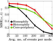
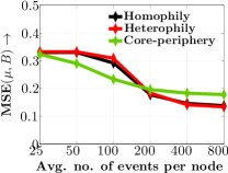
Refer to caption

(a) Temporal parameters, (𝜶,𝑨)𝜶𝑨(\boldsymbol{\alpha},\bm{A})

Refer to caption

(b) Opinion parameters, (𝝁,𝑩)𝝁𝑩(\boldsymbol{\mu},\bm{B})
Figure 5: Performance of model estimation for several 512512512-node kronecker networks in terms of mean squared error between estimated and true parameters. As we feed more messages into the estimation procedure, the estimation becomes more accurate.

Appendix K Twitter dataset description

We used the Twitter search API888https://dev.twitter.com/rest/public/search to collect all the tweets (corresponding to a 2-3 weeks period around the event date) that contain hashtags related to the following events/topics:

  • Politics: Delhi Assembly election, from 9th to 15th of December 2013.

  • Movie: Release of “Avengers: Age of Ultron” movie, from April 28th to May 5th, 2015.

  • Fight: Professional boxing match between the eight-division world champion Manny Pacquiao and the undefeated five-division world champion Floyd Mayweather Jr., on May 2, 2015.

  • Bollywood: Verdict that declared guilty to Salman Khan (a popular Bollywood movie star) for causing death of a person by rash and negligible driving, from May 5th to 16th, 2015.

  • US: Presidential election in the United-States, from April 7th to 13th, 2016.

We then built the follower-followee network for the users that posted the collected tweets using the Twitter rest API999https://dev.twitter.com/rest/public. Finally, we filtered out users that posted less than 200 tweets during the account lifetime, follow less than 100 users, or have less than 50 followers.

Dataset |𝒱|𝒱\mathbf{|\mathcal{V}|} ||\mathbf{|\mathcal{E}|} |(T)|𝑇|\mathcal{H}(T)| 𝔼[𝐦]𝔼delimited-[]𝐦\mathbf{\mathbb{E}[m]} std[m]stddelimited-[]𝑚\text{std}[m]
Tw: Politics 548 5271 20026 0.0169 0.1780
Tw: Movie 567 4886 14016 0.5969 0.1358
Tw: Fight 848 10118 21526 -0.0123 0.2577
Tw: Bollywood 1031 34952 46845 0.5101 0.2310
Tw: US 533 20067 18704 -0.0186 0.7135
Table 1: Real datasets statistics