Kinetics and thermodynamics of reversible polymerization in closed systems

Abstract

Motivated by a recent work on the metabolism of carbohydrates in bacteria, we study the kinetics and thermodynamics of two classic models for reversible polymerization, one preserving the total polymer concentration and the other one not. The chemical kinetics is described by rate equations following the mass-action law. We consider a closed system and nonequilibrium initial conditions and show that the system dynamically evolves towards equilibrium where detailed balance is satisfied. The entropy production during this process can be expressed as the time derivative of a Lyapunov function. When the solvent is not included in the description and the dynamics conserves the total concentration of polymer, the Lyapunov function can be expressed as a Kullback-Leibler divergence between the nonequilibrium and the equilibrium polymer length distribution. The same result holds true when the solvent is explicitly included in the description and the solution is assumed dilute, whether or not the total polymer concentration is conserved. Furthermore, in this case a consistent nonequilibrium thermodynamic formulation can be established and the out-of-equilibrium thermodynamic enthalpy, entropy and free energy can be identified. Such a framework is useful in complementing standard kinetics studies with the dynamical evolution of thermodynamic quantities during polymerization.

I Introduction

The processes of aggregation or polymerization are ubiquitous in Nature, for instance they are present in the polymerization of proteins, the coagulation of blood, or even in the formation of stars. They are often modeled using the classic coagulation equation derived by Smoluchowsky Smoluchowsky (1916a, b). In the forties, P. Flory Flory (1936, 1944) developed his own approach for reactive polymers, with an emphasis on their thermodynamic properties and on their most likely (equilibrium) size distribution. At this time, only irreversible polymerization was considered. The first study of the kinetics of reversible polymerization combining aggregation and fragmentation processes was carried out by Tobolsky et al. Blatz and Tobolsky (1945).

In the seventies, reversible polymerization became a central topic in studies on the association of amino acids into peptides and on the self-assembly of actin. The thermodynamics of assembly of these polymers forms the topic of the now classical treaty by F. Oosawa and S. Asakura Oosawa and Asakura (1975). At about the same time, T. L. Hill made many groundbreaking contributions to non-equilibrium statistical physics and thermodynamics, which allowed him to describe not only the self-assembly of biopolymers like actin and microtubules, but also to address much more complex questions such that of free energy transduction by biopolymers and complex chemical networks Hill (1980). In the eighties, R. J. Cohen and G. B. Benedek Cohen and Benedek (1982) revisited the work of Flory and Stockmayer, by showing that the Flory polymer length distribution is obtained under the assumption of equal free energies of bond formation for all bonds of the same type. They also showed that the kinetically evolving polymer distribution does not have the Flory form in general, and they analyzed the irreversible kinetics of the sol-gel transition.

More recently, the specific conditions on the kernels of aggregation and fragmentation, for which equilibrium solutions of the Flory type exist have been analyzed Aizenman and Bak (1979); van Dongen and Ernst (1984); Vigil (2009). When these conditions are not met, reversible polymerization models admit interesting nonequilibrium phase transitions which are beginning to be investigated Ben-Naim and Krapivsky (2008); Ben-Naim et al. (2010).

The kinetic rate equations of reversible polymerization have broad applications. For instance, in studies on the origin of life, these equations describe the appearance of long polymer chains in the primordial soup Mast et al. (2013). These equations are also used to describe the formation of protein clusters in membranes Turner et al. (2005); Foret (2012); Budrikis et al. (2014) or the self-assembly of carbohydrates (also called glycans) Kartal et al. (2011). In the latter case, a very large repertoire of polymer structures and enzymes are involved in the synthesis and degradation of these polymers. Since it is hardly possible to model all the involved chemical reactions, the authors of this work, Kartal et al., introduced a statistical approach to explain experiments which they have performed using mixtures of such polymers with the appropriate enzymes. Their study underlines the importance of entropy as a driving force in the dynamics of these polymers: under its action a monodisperse solution of such biopolymers, which is placed in a closed reactor with the appropriate enzymes, typically admits an exponential distribution of polymer length as equilibrium distribution, in agreement with maximum entropy arguments used by P. Flory Flory (1936, 1944).

This recent work of Kartal et al. Kartal et al. (2011), motivated us to construct appropriate dynamics which converge on long times towards such equilibrium distributions. In order to complement this with an analysis of the time evolution of thermodynamic quantities, we rely on stochastic thermodynamics (for general reviews see Seifert (2012); Ritort (2008); Jarzynski (2011); Van den Broeck and Esposito (2015)). While this recent branch of thermodynamics has been used extensively in the literature for chemical reaction networks Schnakenberg (1976); Jiu-Li and Van den Broeck (1984); Van den Broeck (1986); Gaspard (2004); Schmiedl and Seifert (2007); Zhang et al. (2012); Ge et al. (2012); Muy et al. (2013) and copolymerization processes Andrieux and Gaspard (2008) at the level of the stochastic chemical master equation, its application to the level of mean-field kinetic rate equations is more recent Polettini and Esposito (2014).

In this paper, we precisely use this level of description based on mean-field rate equations. Implicitly, we assume reaction-limited polymerization. Naturally, if the reactions are too fast or the mobility of the polymers too low, a mean-field approach may not be sufficient and diffusion processes should be accounted for. We focus on two main models of reversible polymerization which reproduce the equilibrium distributions found in Ref. Kartal et al. (2011): In the first one, there is only one conservation law (the total number of monomers) while in the second one, there are two (the total number of monomers and of polymers).

The plan of the paper is as follows. In section II, we study reversible polymerization using general rate equations compatible with one conservation law (the total number of monomers). This is done first at the one-fluid level for which there is no solvent, and then at the two-fluid level, for which there is a solvent. In section III, we apply this general framework to a specific model called String model, in which the rates of aggregation and fragmentation are constant. In section IV, we extend the previous case of reversible polymerization with a single conservation law to the case where there are two conservation laws, namely the total number of monomers and of polymers. In section V, inspired by Ref. Kartal et al. (2011), we study two specific examples of reversible polymerization with two (resp. three) conservation laws, namely the kinetics of glucanotransferases DPE1 (resp. DPE2). For both cases, we construct the dynamics which converge towards the equilibrium distributions found in Ref. Kartal et al. (2011), and we discuss their properties from the standpoint of nonequilibrium thermodynamics.

II Reversible polymerization with one conservation law

We consider a reversible polymerization process made of the following elementary reactions

$$[n]+[m]\stackrel{{\scriptstyle[}}{{k}}_{nm}^{-}]{k_{nm}^{+}}{\rightleftharpoons}[n+m],$$ (1)

where the forward and backward reaction rates, namely $k_{nm}^{-}$ and $k_{nm}^{+}$, are functions of the polymer lengths $n$ and $m$, which are strictly positive and symmetric under a permutation of $n$ and $m$. We denote by $c_{l}$ the concentration of polymers of length $l$. The evolution of this quantity is ruled by

$$\dot{c}_{l}=\frac{1}{2}\sum_{n+m=l>1}(k_{nm}^{+}c_{n}c_{m}-k_{nm}^{-}c_{n+m})-\sum_{n=1}^{\infty}(k_{ln}^{+}c_{l}c_{n}-k_{ln}^{-}c_{l+n}),$$ (2)

which preserves the total concentration of monomers (i.e. the concentration that one would get if all the polymers were broken into monomers) $M=\sum_{l=1}^{\infty}lc_{l}$, but not the total concentration of polymers $c=\sum_{l=1}^{\infty}c_{l}$. Therefore in this case, there is only one conservation law, that of $M$, and one can assume $M=1$. Note also that Eq. 2 generalizes the Becker-Döring equations which describe the dynamic evolution of clusters that gain or loose only one unit at a time Becker and Döring (1935); Ball et al. (1986)

Assuming that the reactions (1) can be treated as elementary, the entropy production rate is given by Kondepudi and Prigogine (1998); de Groot and Mazur (1984)

$$\Sigma=\frac{R}{2}\sum_{n,m}(k_{nm}^{+}c_{n}c_{m}-k_{nm}^{-}c_{n+m})\ln\frac{k_{nm}^{+}c_{n}c_{m}}{k_{nm}^{-}c_{n+m}}\geq 0,$$ (3)

where $R$ is the gas constant. The entropy production rate vanishes when the system reaches equilibrium, i.e. when and only when detailed balance is satisfied:

$$k_{nm}^{+}c^{eq}_{n}c^{eq}_{m}=k_{nm}^{-}c^{eq}_{n+m}.$$ (4)

Using the inequality $\ln x\leq x-1$, which holds for all $x>0$, one easily proves that the following quantity is non-negative, convex and vanishes only at equilibrium

$$L\equiv R\sum_{l}c_{l}\ln\frac{c_{l}}{c_{l}^{eq}}-R(c-c^{eq})\geq 0.$$ (5)

Indeed, by taking the time derivative of $L(t)$ and using the definition of $c$, one obtains $dL/dt=R\sum_{l}\dot{c}_{l}\log c_{l}/c_{l}^{eq}$. Now using (2), we obtain two terms. The first term is

$$\frac{R}{2}\sum_{l}\sum_{n+m=l}(k_{nm}^{+}c_{n}c_{m}-k_{nm}^{-}c_{n+m})\ln\frac{c_{l}}{c_{l}^{eq}}=\frac{R}{2}\sum_{n,m}(k_{nm}^{+}c_{n}c_{m}-k_{nm}^{-}c_{n+m})\ln\frac{c_{n+m}}{c_{n+m}^{eq}},$$

while the second one is

$$-R\sum_{l}\sum_{n}(k_{nl}^{+}c_{n}c_{l}-k_{nl}^{-}c_{n+l})\ln\frac{c_{l}}{c_{l}^{eq}}=-\frac{R}{2}\sum_{n,m}(k_{nm}^{+}c_{n}c_{m}-k_{nm}^{-}c_{n+m})\ln\frac{c_{n}c_{m}}{c_{n}^{eq}c_{m}^{eq}}.$$

By adding these two contributions and using the detailed balance condition of (4) as well as (3), one finds that

$$\Sigma=-R\sum_{l}\dot{c}_{l}\ln\frac{c_{l}}{c_{l}^{eq}}=-\frac{d}{dt}L\geq 0.$$ (6)

This proves that $L$ is a Lyapunov function, i.e. a non-negative, monotonically decreasing function, which vanishes at and only at equilibrium. The existence of such a function implies that the dynamics will always relax to a unique equilibrium state. In Shapiro and Shapley (1965), the authors show that for a chemical system containing a finite number of homogeneous phases, a Gibbs free energy function exists that is minimum at equilibrium. In the context of reacting polymers, a similar free energy function has been derived in Aizenman and Bak (1979). In view of the non-increasing property of this function, the authors have coined the term “F-Theorem”. We discuss below its relation to the more usual H theorem.

II.1 One-fluid version

Until now, our model was exclusively expressed in terms of concentrations and could be used to study non-chemical dynamics such as population dynamics. We now introduce the one fluid model, where the solvent is not described either by choice or because it is absent. The molar fractions of the polymers of length $l$, with $l\geq 1$, are $x_{l}=c_{l}/c$ while the Lyapunov function is

$$L=Rc\sum_{l\geq 1}x_{l}\ln\frac{x_{l}}{x_{l}^{eq}}+Rc\ln\frac{c}{c_{eq}}-R(c-c^{eq})\geq 0.$$ (7)

It is important to note that this Lyapunov function is in general distinct from the relative entropy or Kullback-Leibler divergence between the distribution $x_{l}$ and $x_{l}^{eq}$, which represents only the first term in Eq. (5). The reason for this difference is that $c_{l}$, contrary to $x_{l}$, cannot always be interpreted as a probability since its norm is not always conserved. The two quantities become however equivalent (i.e. they only differ by a constant) when the total concentration of polymers $c(t)$ is constant in time. If furthermore -$\sum_{l}x_{l}\ln x_{l}^{eq}$ is constant in time (the meaning of this assumption will become clear in the two fluid model), then the negative of the Shannon entropy (which is related to the classic notion of free energy of mixing introduced in Flory (1936, 1944) as explained in Ben-Naim (2006))

$$S_{Sh}=-R\sum_{l\geq 1}x_{l}\ln x_{l},$$ (8)

becomes a Lyapunov function and (6) reduces to the famous Boltzmann “H theorem”.

II.2 Two-fluid version

In order to make contact with thermodynamics, we now introduce the two fluid model which includes the solvent explicitly in the list of chemical species. Then, the molar fraction of the polymer of length $l$ becomes $y_{l}(t)=c_{l}(t)/C(t)$, which importantly is now defined with respect to the total concentration of all species including the (time-independent) solvent concentration $c_{0}$ (water for instance): $C(t)=\sum_{l\geq 0}c_{l}(t)=c(t)+c_{0}$, where $c(t)=\sum_{l\geq 1}c_{l}(t)$. If there is no solvent, $c_{0}=0$ and one recovers the molar fraction of the previous section which was denoted by $x_{l}$. In dilute solution, since $y_{0}$ is very close to one and the other $y_{l}$ are much smaller, $C(t)$ becomes almost constant: $C\approx c_{0}$. The chemical potential of a polymer of length $l$ in a dilute solution is defined by $\mu_{l}=\mu^{0}_{l}+RT\ln y_{l}$, where $\mu^{0}_{l}=h^{0}_{l}-Ts^{0}_{l}$ is the standard reference chemical potential and $h^{0}_{l}$ and $s^{0}_{l}$ are the standard enthalpy and entropy respectively. We restrict ourselves here to ideal solutions, and by this we assume that this form of chemical potential applies not only to the polymers ($l\neq 0$) but also to the solvent. An interesting study of the effect of non-ideality on the time evolution thermodynamic quantities during reversible polymerization can be found in Ref. Stier (2006).

Let us define the intensive enthalpy function as

$$H=\sum_{l\geq 0}y_{l}h_{l}^{0},$$ (9)

and the entropy function of this two-fluid model as

$$S=\sum_{l\geq 0}y_{l}(s_{l}^{0}-R\ln{y_{l}}).$$ (10)

Their extensive counterparts are ${\cal H}=CH$ and ${\cal S}=CS$. In Eq. (10), the first term proportional to $s_{l}^{0}$ therefore represents the entropic contribution due to the disorder in the internal degrees of freedom of each polymer, while the second term represents the nonequilibrium entropy in the distribution of the variables $y_{l}$ Gaspard (2004). Let us introduce the intensive free enthalpy

$$G=H-TS=\sum_{l\geq 0}y_{l}\mu_{l},$$ (11)

where we used the definition of the chemical potential in the last equality, and its extensive counterpart ${\cal G}=CG$.

Since the change of chemical potential associated to each reaction must vanish at equilibrium, i.e. $\Delta\mu=\mu_{n+m}-\mu_{n}-\mu_{m}=0$, using the definition of the chemical potential, we find that

$$RT\ln\frac{y^{eq}_{n+m}}{y^{eq}_{n}y^{eq}_{m}}=-(\mu^{0}_{n+m}-\mu^{0}_{n}-\mu^{0}_{m}).$$ (12)

Combining (12) with (4), we obtain that the kinetic constants must satisfy local detailed balance

$$RT\ln\frac{k_{nm}^{+}C^{eq}}{k_{nm}^{-}}=-(\mu^{0}_{n+m}-\mu^{0}_{n}-\mu^{0}_{m}),$$ (13)

where $C^{eq}$ denotes the equilibrium value taken by $C$. We note that since the chemical reactions do not involve the solvent, we formally define the rate constants with any zero subscript ($n$ or $m$) to be zero. Naturally, Eq. (13) is not applicable in this case. The validity of Eq (13) relies on two main assumptions: the first one is that of dilute solutions, while the second one is the ideality of the heat bath. The latter assumption means that there are no hidden degrees of freedom which can dissipate energy in the chemical reactions under consideration, which implies in particular that these reactions must be elementary.

Using the definitions of the enthalpy and entropy functions, we find that

$$\frac{d{\cal H}}{dt}=\frac{1}{2}\sum_{n,m}(k_{nm}^{+}c_{n}c_{m}-k_{nm}^{-}c_{n+m})\big{(}h_{n+m}^{0}-h_{n}^{0}-h_{m}^{0}\big{)}$$ (14)

and

$$\frac{d{\cal S}}{dt}=\frac{1}{2}\sum_{n,m}(k_{nm}^{+}c_{n}c_{m}-k_{nm}^{-}c_{n+m})\big{(}s_{n+m}^{0}-s_{n}^{0}-s_{m}^{0}+R\ln\frac{y_{n}y_{m}}{y_{n+m}}\big{)}.$$ (15)

As a result, one finds that

$$\frac{d{\cal G}}{dt}=\frac{RT}{2}\sum_{n,m}(k_{nm}^{+}c_{n}c_{m}-k_{nm}^{-}c_{n+m})\ln\frac{y_{n+m}y^{eq}_{n}y^{eq}_{m}}{y^{eq}_{n+m}y_{n}y_{m}}=RT\sum_{l}{\dot{c}}_{l}\ln\frac{y_{l}}{y^{eq}_{l}},$$ (16)

where we used Eq. (12) to obtain the last equality. By including the solvent in the sum, as the term corresponding to $l=0$, we have $\sum_{l\geq 0}y_{l}=1$ and therefore $\sum_{l\geq 0}{\dot{y}}_{l}=0$; thus we can rewrite the above equation as

$$\frac{d{\cal G}}{dt}=RT\frac{d}{dt}\bigg{(}C\sum_{l\geq 0}y_{l}\ln\frac{y_{l}}{y^{eq}_{l}}\bigg{)}.$$ (17)

The entropy production (3), using (13) and the chemical potential definition, may be written as

$$T\Sigma=-\frac{1}{2}\sum_{n,m}(k_{nm}^{+}c_{n}c_{m}-k_{nm}^{-}c_{n+m})\big{(}\mu_{n+m}-\mu_{n}-\mu_{m}-RT\ln\frac{C}{C^{eq}}\big{)}\geq 0.$$ (18)

Using Eq. (14) and Eq. (15), it can be rewritten as

$$T\Sigma=-\frac{d}{dt}\bigg{[}{\cal H}-T{\cal S}-RTC\ln\frac{C}{C^{eq}}-RT\big{(}C^{eq}-C\big{)}\bigg{]}\geq 0.$$ (19)

The first term is the heat flow, the second the entropy change and the third and fourth terms represent a contribution due to the change in the total concentration. It is important to note that within the two-fluid model with ideal solutions, since $C(t)$ is essentially constant, these latter two contributions are negligible. Neglecting these terms, the entropy production can be expressed as the change in free energy which is also equal to a change in Kulback-Leibler divergence between the nonequilibrium and the equilibrium polymer distribution

$$T\Sigma=-\frac{d{\cal G}}{dt}=-RT\frac{d}{dt}\big{(}C\sum_{l\geq 0}y_{l}\ln\frac{y_{l}}{y_{l}^{eq}})\geq 0.$$ (20)

We finally note that when all the polymerization reactions are neutral from a standard chemical potential standpoint i.e. when $\mu^{0}_{n+m}=\mu^{0}_{n}+\mu^{0}_{m}$ for all $n,m$, one has that

$$\frac{d{\cal G}}{dt}=RT\frac{d}{dt}\big{(}\sum_{l\geq 0}c_{l}\ln y_{l}\big{)}=RT\frac{d}{dt}\big{(}C\sum_{l\geq 0}y_{l}\ln y_{l}\big{)},$$ (21)

which together with Eq. (17) implies $d_{t}(C\sum_{l}y_{l}\ln y_{l}^{eq})=0$. Since $C$ can be assumed constant, the Lyapunov function can be expressed only in terms of the Shannon entropy constructed from $y_{l}$ instead of the full KL divergence. The dynamics can then be compared to a Boltzmann equation where the relaxation to equilibrium is purely driven by the maximization of the Shannon entropy, as in the H-Theorem.

III Application to the String model

As a simple realisation of the reversible polymerization given by Eq. (1), we now consider the String model which assumes constant rates of aggregation and fragmentation, independent of the length of the reacting polymers. Following Ben-Naim et al. (2010), we choose $k_{nm}^{+}=2$ and $k_{nm}^{-}=2\lambda$. From Eq. (2), the dynamics follows

$$\dot{c}_{l}=\sum_{i+j=l}c_{i}c_{j}+2\lambda\sum_{j>l}c_{j}-2c_{l}c-\lambda(l-1)c_{l},$$ (22)

where we used the fact that $(l-1)$ combinations of $i$ and $j$ satisfy the relation $i+j=l$. The detailed balance condition defining equilibrium implies that $c_{i}^{eq}c_{j}^{eq}=\lambda c_{i+j}^{eq}$, which admits one parameter solutions of the form $c_{l}^{eq}=\lambda\beta^{l}$. Assuming the total monomer concentration to be $M=\sum_{l}lc_{l}=1$, one finds

$$\beta=1+\frac{\lambda}{2}-\sqrt{\lambda+\frac{\lambda^{2}}{4}},$$ (23)

since the solution $c_{l}$ must decay at large $l$.

III.1 One-fluid version of the String model

The evolution of the length distribution in the String model can be obtained as a function of time by explicit numerical integration. The results, starting from time $t=0$, are shown in Fig. 1.

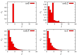
Figure 1: Evolution of the size distribution of polymers $c_{l}$ for the String model at different times $t=0$, $t=0.2$, $t=0.5$ and $t=1$ starting with a monodisperse distribution with characteristic length $l=4$ at time $t=0$. The transition rates are constant and correspond to $\lambda=1$. A rapid convergence towards an exponential distribution can already be seen after a time $t\simeq 1$.

The evolution equation (22) can be solved using an exponential ansatz of the form Ben-Naim et al. (2010)

$$c_{l}(t)=(1-a(t))^{2}a^{l-1}(t),$$ (24)

which satisfies the conservation of total number of monomers. The resulting differential equation for $a(t)$ is $\dot{a}=(1-a)^{2}-\lambda a$. This equation can be easily solved with a monomer-only initial condition, $c_{l}=\delta_{l,1}$, which translates into the condition $a(0)=0$. Unfortunately, the exponential ansatz cannot be used to describe more general initial conditions, which cannot be accounted for by such a simple $l$-independent condition on $a(0)$. For the monomer-only initial condition, the following explicit solution is obtained:

$$a(t) = \frac{1-\exp{\{-(\alpha_{+}-\alpha_{-})t\}}}{\alpha_{+}-\alpha_{-}\exp{\{-(\alpha_{+}-\alpha_{-})t\}}}$$ (26)

$$\alpha_{\pm}\equiv 1+\frac{\lambda}{2}\pm\sqrt{\lambda+\frac{\lambda^{2}}{4}},$$

where the two roots $\alpha_{-}$ and $\alpha_{+}$ are related by $\alpha_{-}\alpha_{+}=1$. At long times, the RHS of Eq. (26) tends towards $1/\alpha_{+}=\alpha_{-}=\beta$, so that the system approaches the equilibrium distribution $c_{l}(\infty)=c_{l}^{eq}=(1-\alpha_{-})^{2}(\alpha_{-})^{l-1}$.

Using (26), one can obtain the explicit time evolution of the quantities of interest: The total polymer concentration is time-dependent and reads

$$c(t)=\sum_{l\geq 1}c_{l}(t)=1-a(t).$$ (27)

The Shannon entropy at the one fluid level, and defined in Eq. (8), is given by

$$S_{Sh}(t)=-\ln{(1-a(t))}-\frac{a(t)}{1-a(t)}\ln{a(t)},$$ (28)

and reaches its equilibrium value $S_{Sh}(\infty)=-\ln{(1-\alpha_{-})}-(\alpha_{-}/(1-\alpha_{-}))\ln{\alpha_{-}}$ for long times. Its rate of change is

$$\dot{S}_{Sh}=-a(t)\ln{a(t)}+\lambda\frac{a(t)}{(1-a(t))^{2}}\ln{a(t)},\\$$ (29)

while the entropy production rate given by Eq. (6) is

$$\Sigma=R\left(2\ln\frac{1-a(t)}{1-\alpha_{-}}-\ln\frac{a(t)}{\alpha_{-}}\right)\left((1-a(t))^{2}-\lambda a(t)\right).$$ (30)

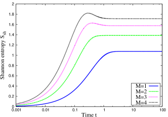
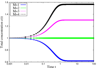
Figure 2: Left: Shannon entropy of the one fluid version of the String model, $S_{Sh}$, as a function of time. The various curves represent different initial conditions of the form $c_{l}(t=0)=\delta_{lM}$, for different total monomer concentration $M=1,2,3$ and $4$. Right: Total polymer concentration $c(t)$ for the same initial conditions, as found by numerical integration of kinetic equations (solid line) or from an exact expression using Eq. (36) (symbols). Both figures have been done with the same rates as Fig. 1.

For completeness, we also discuss an approach using generating functions to study the String model without resorting to the exponential ansatz which is restricted to the monomer-only initial condition. The full dynamics remains nevertheless complex to solve within this approach. Introducing the generating function $\chi(z,t)=\sum_{l\geq 1}c_{l}(t)z^{l}$ and using Eq. (22), we obtain the dynamical equation

$$\frac{\partial\chi}{\partial t}=\chi^{2}-2c\chi+2\lambda\sum_{l}\sum_{j>l}c_{j}z^{l}-\lambda\left(z\frac{\partial\chi}{\partial z}-\chi\right),$$ (31)

which can be simplified since for $|z|<1$, $\sum_{l}\sum_{j>l}c_{j}z^{l}=(cz-\chi)/(1-z)$, so that

$$\frac{\partial\chi}{\partial t}=\chi^{2}-2c\chi+2\lambda\frac{cz-\chi}{1-z}-\lambda\left(z\frac{\partial\chi}{\partial z}-\chi\right).$$ (32)

The stationary solution of this differential equation, i.e. the solution of $\partial\chi/\partial t=0$ has the following form:

$$\chi^{eq}(z)\equiv\chi(z,t\rightarrow\infty)=\frac{\lambda c^{eq}z}{c^{eq}(1-z)+\lambda},$$ (33)

which satisfies $\chi(1,t\rightarrow\infty)=\sum_{l\geq 1}c_{l}=c^{eq}$ and $\chi^{\prime}(1,t\rightarrow\infty)=c^{eq}(\lambda+c^{eq})/\lambda$. Since $M=\sum_{l\geq 1}lc_{l}=\chi^{\prime}(1,t\rightarrow\infty)=1$, one recovers the equilibrium state obtained before, namely $c^{eq}=1-\beta$, with $\beta$ given by Eq. (23). For an arbitrary $M$, one deduces from Eq. (33) that the equilibrium polymer length distribution is $c_{l}^{eq}=\lambda\alpha^{l}$, where $\alpha=c^{eq}/(\lambda+c^{eq})$. With our choice of initial condition of the form $c_{l}(0)=\delta_{lM}$, we have $\sum_{l\geq 1}lc_{l}=M$. Therefore, the equilibrium solution is

$$c_{l}^{eq}=\frac{(c^{eq})^{2}}{M}\bigg{(}1-\frac{c^{eq}}{M}\bigg{)}^{l-1}.$$ (34)

Besides the stationary solution, it is also possible to obtain analytically the evolution of the total concentration $c(t)$. To show this, we take the limit $z\rightarrow 1$ in Eq. (32). Using l’Hospital rule, we obtain

$$\dot{c}=-c^{2}+\lambda(M-c).$$ (35)

The explicit solution of Eq. (35) for $c(0)=1$, as imposed by our choice of initial conditions of the form $c_{l}(t=0)=\delta_{lM}$ is

$$c(t)=\frac{\Delta}{2}\tanh\left(\frac{t}{2}\Delta+\operatorname{arctanh}\frac{\lambda+2}{\Delta}\right)-\frac{\lambda}{2}.$$ (36)

where $\Delta=\sqrt{\lambda(\lambda+4M)}$. One can verify that Eq. (27) is recovered for the monomer only initial condition, $M=1$, as expected. Furthermore, one recovers that $c(t)$ tends towards $c^{eq}=(\Delta-\lambda)/2$ as $t\to\infty$, which is the equilibrium concentration entering in Eqs. (33) and (34).

Incidentally, one may wonder whether this behavior of the total concentration agrees with the predictions of Ref. Oosawa and Asakura (1975) regarding the notion of critical concentration in reversible polymerization. This is indeed the case: if one evaluates the concentration of monomers $c_{1}$ as a function of $M$, with Eq (34) and eliminating $c^{eq}$ using the above expression, one finds a function of $M$ which first increases rapidly and then reaches a plateau for $M\geq\lambda$. Naturally, this is not a sharp transition but rather a cross-over between two regimes. One can also look at the average length of the polymer $M/c^{eq}$ which increases significantly when $M$ becomes larger than $\lambda$. Both features indicate that $\lambda$ represents the critical concentration of this model Oosawa and Asakura (1975).

As shown in the right part of Fig. 2, which has been obtained by explicit numerical integration, the polymer concentration $c(t)$ either decreases as a function of time for the monomer only initial condition ($M=1$) or increases as a function of time when the initial condition corresponds to polymers of length 3 or above ($M\geq 3$), while it remains constant for the case of dimers ($M=2$). Intuitively, when the initial condition is monomer-only ($M=1$), there is mainly aggregation of monomers, so that the net concentration must decrease with time. On the other hand, if the initial solution consists of long polymers ($M>2$), the probability of fragmentation is higher than that of aggregation. As a result, the total concentration must increase with time. For dimer-only initial condition ($M=2$), the probabilities of fragmentation is same as that of aggregation, so that the net concentration stays constant. As a result of this time dependence of $c(t)$, we also see in the left part of Fig. 2, that the Shannon entropy $S_{Sh}$ does not always increase monotonically as a function of time. It does so for $M\leq 2$ but not for $M>2$, where it presents an overshoot before reaching its equilibrium value. Such an overshoot reveals that the Shannon entropy is not a Lyapunov function $L$ as discussed in the previous section.

III.2 Two-fluid version of the String model

One of the main difference between the two fluid approach as compared with the previous one with a single fluid, is the existence of the local detailed balance condition, namely Eq. (13), which connects the rate constants to the difference of standard chemical potentials. Further, the specific form of the standard chemical potentials enters in the equilibrium length distribution of the polymers and in the kinetics of the self-assembly process.

For instance, if the polymers self-assemble linearly, the standard chemical potential of a polymer of length $l$, $\mu_{l}^{0}$ for $l\geq 1$, may be written as $\mu_{l}^{0}=-(l-1)\alpha RT$, where $\alpha RT$ represents the bond energy between two monomers Israelachvili (1992). For such a model, a reaction is neutral from the point of view of chemical potentials, i.e. when $\mu_{n+m}^{0}=\mu_{n}^{0}+\mu_{m}^{0}$, when the polymer chain is sufficiently long so that $\mu_{l}^{0}\simeq-l\alpha RT$. From Eq. (13), it follows that

$$RT\ln\frac{k_{nm}^{+}C^{eq}}{k_{nm}^{-}}=-(\mu^{0}_{n+m}-\mu^{0}_{n}-\mu^{0}_{m})=\alpha RT,$$ (37)

which then implies a relation between the parameter $\lambda$ defined earlier as the ratio of the rate constants (assumed constant) and the parameter $\alpha$, namely $\lambda=e^{-\alpha}C^{eq}$.

Since we introduced $\alpha RT$ as bond energy between two consecutive monomers, the simplest choice is to assume that $\mu_{l}^{0}$ leads to a molar enthalphy $h_{l}^{0}=-(l-1)\alpha RT$, and a molar entropy $s_{l}^{0}$ which is assumed to be negligible with respect to the enthalpy part due to bond formation. With this choice, one finds the following contribution of the polymer to the enthalpy:

$$H_{1}=-\alpha RT\sum_{l\geq 1}y_{l}(l-1){=-\alpha RT(M-c(t))}.$$ (38)

As discussed previously, at the two fluid level, this should be complemented by the contribution of the solvent to obtain the enthalpy $H$. Similarly, the system entropy $S$, which contains both contributions, is

$$S=-R\sum_{l\geq 0}y_{l}\ln{y_{l}}.$$ (39)

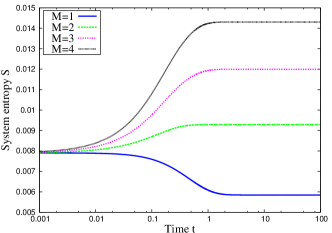
Figure 3: System entropy $S$ for the two-fluid version of the String model as a function of time. The various curves represent different initial conditions as in Fig. 2. The solvent concentration is $c_{0}=1000$ and the transition rates are the same as in Fig. 1.

In Fig. 3, we show this entropy function as a function of time for different initial conditions in units of $R$. At $t=0$, it equals approximately $(1+\ln c_{0})/c_{0}$, and it converges towards the equilibrium value of the entropy at large times. For $M>1$, the entropy increases monotonically whereas we see that it decreases for $M=1$. As in the case of the one fluid model, this decrease is not inconsistent since the entropy is not the Lyapunov function. We note that the non-monotonicity that was present in the one-fluid model in Fig. 2 for $M>1$ is absent in the two-fluid case.

If the monomers were to assemble in the polymer in a different way, for instance in the form of disks instead of linear chains, the standard chemical potentials would be different. In such a case, under similar assumptions as above, these chemical potentials would be of the form $\mu_{l}^{0}=-(l-\sqrt{l})\alpha RT$, where $\alpha$ is again some constant characteristic of the monomer-monomer and monomer-solvent interaction Israelachvili (1992). The term in $\sqrt{l}$ represents the contribution of the surface energy of the cluster of size $l$. This term necessarily implies that the rate constants $k_{nm}^{+}$, $k_{nm}^{-}$ must depend on $n$ and $m$ in order to satisfy the local detailed balance condition Eq. 13. For such a case, the above derivation of a simple exponential for the equilibrium distribution would no longer hold and both the equilibrium and the dynamics will would be more complex.

IV Reversible polymerization model with two conservation laws

As done previously in section II for a reversible polymerization model with only one conservation law, namely the total monomer concentration $M$, we now carry out a similar analysis for a different class of models with two conservation laws, namely $M$ and the total concentration of polymers or clusters, $c$. Clearly, the latter quantity varies in time in the String model because some exchange process in Eq. (1) produce clusters of zero length for some $n$ or $m$. In order to construct a model, which conserves the total number of clusters, one needs to forbid such transitions. One simple way to achieve this is to consider the kinetic model

$$[n]+[m]\stackrel{{\scriptstyle[}}{{k}}_{nm}]{}{\rightarrow}[n+1]+[m-1],$$ (40)

with the condition $n\geq 1$ and $m\geq 2$, where the latter inequality precisely prevents the forbidden transitions. It is easy to check that now the total concentration of the polymers, $c=\sum_{l}c_{l}$, as well as the total monomer concentration $M=\sum_{l}lc_{l}$, remain constant in time. Another important observation is that this model is fully reversible even if we do not indicate backward reactions explicitly. Indeed, it would be redundant to do so, since backward reactions are already included in the forward reactions via an appropriate choice of the indexes $(n,m)$. As done in the previous section, we first present a general proof of convergence to equilibrium and then we make contact with thermodynamics by introducing chemical potentials in dilute solutions.

The equation for the rate of change of concentration for polymer size distribution is

$$\dot{c}_{l} =\Theta(l-2)\sum_{n=1}^{\infty}[k_{l-1,n+1}c_{n+1}c_{l-1}-k_{nl}c_{n}c_{l}]+\sum_{m=2}^{\infty}[k_{m-1,l+1}c_{l+1}c_{m-1}-k_{lm}c_{l}c_{m}],$$ (41)

where the Heaviside function $\Theta(l-2)$ equals 1 for $l\geq 2$, and is zero otherwise.

Assuming again elementary reactions, the entropy production rate $\Sigma$ is

$$\Sigma=\frac{R}{2}\sum_{n\geq 1,m\geq 2}[k_{nm}c_{n}c_{m}-k_{m-1,n+1}c_{n+1}c_{m-1}]\ln\frac{k_{nm}c_{n}c_{m}}{k_{m-1,n+1}c_{n+1}c_{m-1}}\geq 0,$$ (42)

which vanishes when the detailed balance condition holds, i.e. in equilibrium:

$$k_{nm}c_{n}^{eq}c_{m}^{eq}=k_{m-1,n+1}c_{n+1}^{eq}c_{m-1}^{eq}.$$ (43)

Following a procedure similar to that of section II, one can show that, since $c$ is constant, the relative entropy between the distribution $x_{l}$ and $x_{l}^{eq}$

$$L=R\sum_{l}c_{l}\ln\frac{c_{l}}{c^{eq}_{l}}=Rc\sum_{l}x_{l}\ln\frac{x_{l}}{x^{eq}_{l}},$$ (44)

is a Lyapunov function. Indeed, this quantity is convex, non-negative (by the inequality $\ln x<x-1$), and a monotonically decreasing function vanishing at equilibrium. This latter property follows from

$$\frac{dL}{dt}=R\sum_{l}\dot{c}_{l}\ln\frac{c_{l}}{c^{eq}_{l}},$$ (45)

which using Eq. (41) and the detailed balance condition of Eq. (43) gives

$$\frac{dL}{dt}=R\sum_{n\geq 1,l\geq 2}k_{nl}c_{n}c_{l}\ln\frac{k_{l-1,n+1}c_{n+1}c_{l-1}}{k_{nl}c_{n}c_{l}}.$$ (46)

After symmetrizing this sum, we recover that $\Sigma=-dL/dt\geq 0$. This result is equivalent to Eq. (6) in presence of the additional conservation law $\dot{c}=0$. This system will therefore relax to a unique equilibrium state, where $\Sigma$ vanishes.

We now turn to the two fluid version of the model. As in section II.2, for the two fluids model the molar fraction of a polymer of length $l$ is $y_{l}(t)=c_{l}(t)/C$, where $C=c+c_{0}$ is again a constant. The change in chemical potential during the reaction (40) is given by

$$\Delta\mu =\mu_{n+1}+\mu_{m-1}-\mu_{n}-\mu_{m}$$

$$=\mu^{0}_{n+1}+\mu^{0}_{m-1}-\mu^{0}_{n}-\mu^{0}_{m}+RT\ln\frac{y_{n+1}y_{m-1}}{y_{n}y_{m}}.$$ (47)

Since at equilibrium $\Delta\mu=0$, using (43), we get that

$$\mu_{n}^{0}+\mu_{m}^{0}-\mu^{0}_{n+1}-\mu^{0}_{m-1}=RT\ln\frac{y^{eq}_{n+1}y^{eq}_{m-1}}{y^{eq}_{n}y^{eq}_{m}}=RT\ln\frac{k_{nm}}{k_{m-1,n+1}}.$$ (48)

The enthalpy change (9) can be written as

$$\frac{d{\cal H}}{dt} =C\frac{d}{dt}\sum_{l}y_{l}h^{0}_{l}=\sum_{l}\dot{c}_{l}h^{0}_{l}$$

$$=\sum_{n\geq 1,m\geq 2}(k_{m-1,n+1}c_{n+1}c_{m-1}-k_{nm}c_{n}c_{m})(h^{0}_{n}+h^{0}_{m})$$

$$=\sum_{n\geq 1,m\geq 2}(k_{nm}c_{n}c_{m}-k_{m-1,n+1}c_{m-1}c_{n+1})(h^{0}_{m-1}+h^{0}_{n+1})$$

$$=\frac{1}{2}\sum_{n\geq 1,m\geq 2}(k_{nm}c_{n}c_{m}-k_{m-1,n+1}c_{n+1}c_{m-1})(h^{0}_{m-1}+h^{0}_{n+1}-h^{0}_{n}-h^{0}_{m})$$ (49)

and the entropy change (10) as

$$\frac{d{\cal S}}{dt} =C\frac{d}{dt}\sum_{l\geq 0}y_{l}(s^{0}_{l}-R\ln y_{l})=\sum_{l\geq 0}\dot{c}_{l}(s^{0}_{l}-R\ln c_{l})$$

$$=\sum_{n\geq 1,m\geq 2}(k_{nm}c_{n}c_{m}-k_{m-1,n+1}c_{n+1}c_{m-1})\left(s^{0}_{m-1}+s^{0}_{n+1}-s^{0}_{n}-s^{0}_{m}+R\ln\left[\frac{y_{n}y_{m}}{y_{n+1}y_{m-1}}\right]\right).$$ (50)

Since the entropy production can be rewritten as

$$T\Sigma =\frac{1}{2}RT\sum_{n\geq 1,m\geq 2}[k_{nm}c_{n}c_{m}-k_{m-1,n+1}c_{n+1}c_{m-1}]\ln\frac{k_{nm}c_{n}c_{m}}{k_{m-1,n+1}c_{n+1}c_{m-1}}$$

$$=\frac{1}{2}\sum_{n\geq 1,m\geq 2}[k_{nm}c_{n}c_{m}-k_{m-1,n+1}c_{n+1}c_{m-1}]\left[\mu^{0}_{n}+\mu^{0}_{m}-\mu^{0}_{n+1}-\mu^{0}_{m-1}+RT\ln\frac{y_{n}y_{m}}{y_{n+1}y_{m-1}}\right]$$

$$=\frac{1}{2}\sum_{n\geq 1,m\geq 2}(k_{nm}c_{n}c_{m}-k_{m-1,n+1}c_{n+1}c_{m-1})(\mu_{n}+\mu_{m}-\mu_{n+1}-\mu_{m-1}),$$ (51)

we can express it, as in (20), as

$$T\Sigma=-\frac{d}{dt}({\cal H}-T{\cal S})=-\frac{d{\cal G}}{dt}=-R\frac{d}{dt}\big{(}C\sum_{l\geq 0}y_{l}\ln\frac{y_{l}}{y_{l}^{eq}})=-\frac{dL}{dt}\geq 0.$$ (52)

To summarize, we recover exactly the same results as in section II, provided we treat the total polymer concentration $c$ as a constant.

V Application to the kinetics of glucanotransferases DPE1 and DPE2

In this section, we consider the polymerization of glycans by two enzymes studied by Kartal et al. Kartal et al. (2011), namely the glucanotransferases DPE1 and DPE2. We show how to construct dynamical models that are compatible with the equilibrium polymer length distributions that they found and we study the dynamics of the Shannon entropy for various initial conditions.

V.1 Kinetics of glucanotransferases DPE1

Let us assume that the initial condition is not purely made of monomers, since the solution of Ref. Kartal et al. (2011) becomes singular in that limit (see Eq. (4) on P3 of Ref. Kartal et al. (2011) when the parameter $DP_{in}=1$ for instance), and let us construct an appropriate dynamics, choosing for simplicity constant rates $k_{nm}=\kappa$ independent of $n$ and $m$.

Using Eq. (41), we have for $l\geq 2$,

$$\frac{dc_{l}}{dt}=\kappa[c\left(c_{l+1}+c_{l-1}-2c_{l}\right)-c_{1}c_{l-1}+c_{1}c_{l}],$$ (53)

where the second term forbids transitions from $[1]+[l-1]$ to $[0]+[l]$, while the last term forbids transitions from $[1]+[l]$ to $[0]+[l+1]$. Similarly, for $c_{1}$, the evolution is

$$\frac{dc_{1}}{dt}=\kappa[c\left(c_{2}-c_{1}\right)+c_{1}^{2}].$$ (54)

It is straightforward to verify that this dynamics has two conservation laws, namely $\sum_{l\geq 1}c_{l}=c$ and $\sum_{l\geq 1}lc_{l}=M$.

Introducing the generating function $\chi(z,t)=\sum_{l\geq 1}c_{l}(t)z^{l}$ as in section III leads once again to a set of equations for the dynamics which unfortunately can not be solved analytically. However, it enables us to find an explicit solution for the equilibrium state:

$$\chi^{eq}(z)\equiv\chi(z,t\rightarrow\infty)=\frac{c^{2}z}{M-Mz+cz},$$ (55)

which means that the size distribution $c_{l}$ tends towards the following equilibrium distribution for $l\geq 1$:

$$c^{eq}_{l}=\frac{c^{2}}{M}\left(1-\frac{c}{M}\right)^{l-1},$$ (56)

where the total polymer concentration $c$ is now fixed by the initial condition. We note that the form of the equilibrium distribution is the same as that of the String model, but $c^{eq}$ in Eq. (34) is different from $c(t=0)$, whereas in the present DPE1 model they are the same. Our equilibrium solution (56) also matches that of Kartal et al. found for the polymerization of glycans by glucanotransferases DPE1 Kartal et al. (2011). In this reference, the authors use the polymer fractions $x_{l}$, where $l$ stands for the number of linkages in one cluster, rather than our cluster distribution $c_{l}$. They are related by $x_{l}=c_{l+1}/c$. Their conservation laws therefore read $\sum_{l\geq 0}x_{l}=1$ and $\sum_{l\geq 0}lx_{l}=DP_{ini}-1$, where $DP_{ini}$ stands for the initial degree of polymerization. The latter is related to $c$ by $DP_{ini}=M/c$, and the relation $1-c/M=e^{-\beta}$ matches Eq. (4) of Kartal et al.

The Shannon entropy, Eq. (8), at equilibrium and in $R$ units, reads

$$S_{Sh}(t\rightarrow\infty)=\frac{M}{c}\ln\frac{M}{c}-\left(\frac{M}{c}-1\right)\ln\left(\frac{M}{c}-1\right),$$ (57)

and has the standard form of a mixing entropy. Note that the case of monomer-only initial condition, namely $c=M=1$, is singular since no evolution is possible from this initial condition according to the present dynamics. In this case, the Shannon entropy stays at zero, for all times $t$, whereas for other initial conditions it increases monotonically as shown in Fig. 4.

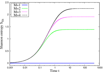
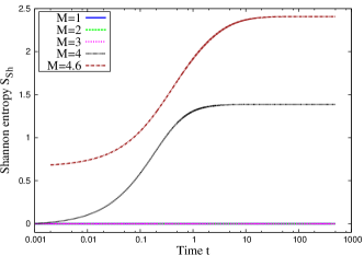
Figure 4: Left (resp. right): Evolution of the Shannon entropy $S_{Sh}$ for the one fluid DPE1 (resp. DPE2) model with time for different initial conditions. For both plots, the curves for $M=1,2,3$ and $4$ correspond to initial conditions of the form $c_{l}(0)=\delta_{lM}$. For the DPE2 plot on the right, $M=4.6$ corresponds to an initial condition of the form $c_{l}(0)=0.4\delta_{l1}+0.6\delta_{l7}$. Note that when $M=1$ for DPE1 and $M=1,2$ and $3$ for DPE2, the Shannon entropy is zero since no evolution is possible from the initial condition. We have chosen the constant rate $\kappa=1$.

V.2 Application to the kinetics of glucanotransferase DPE2

As discussed by Kartal et al. Kartal et al. (2011), the enzyme DPE2 introduces an additional constraint with respect to the enzyme DPE1. This additional constraint, which imposes a conservation of the total number of monomers and dimers, reads in our notations $c_{1}+c_{2}=pc$, where $p$ depends on the initial conserved total number of molecules of maltose (corresponding to $c_{2}$) and glucose (corresponding to $c_{1}$). This additional constraint requires a modification of the dynamical evolution equations. We propose the following modification:

$$\frac{dc_{1}}{dt} = \kappa[c\left(c_{2}-c_{1}\right)+c_{1}^{2}-c_{2}^{2}+c_{1}c_{3}],$$ (58)

$$\frac{dc_{2}}{dt} = -\frac{dc_{1}}{dt},$$ (59)

$$\frac{dc_{3}}{dt} = \kappa[c(c_{4}-c_{3})-c_{2}c_{4}+c_{1}c_{3}+c_{3}^{2}],$$ (60)

and for $l\geq 4$,

$$\frac{dc_{l}}{dt} = \kappa[c\left(c_{l+1}+c_{l-1}-2c_{l}\right)-c_{1}c_{l-1}-c_{2}c_{l+1}$$ (61)

$$-c_{3}c_{l-1}+(c_{1}+c_{2}+c_{3})c_{l}],$$

As in the case of DPE1, one can solve the stationary state of this equation by means of generating functions. One obtains the following stationary generating function:

$$\chi^{eq}(z)\equiv\chi(z,t\rightarrow\infty)=\frac{\left[c_{1}c_{2}-cc_{1}-z^{2}\left(c_{1}c_{2}-cc_{2}+cc_{3}\right)\right]z}{c(z-1)-c_{1}z+c_{2}-c_{3}z}.$$ (62)

One obtains from this $c_{1}=pc/(1+f)$ and $c_{2}=c_{1}f=fpc/(1+f)$ with $f=(c-c_{1}-c_{3})/(c-c_{2})$, and for $l\geq 3$, $c_{l}=c_{3}f^{l-3}$ with $c_{3}=(1-p)(1-f)c$. In other words, for DPE2, the equilibrium distribution is again exponential but only for length $l\geq 3$, for $l<3$ the ratio of $c_{2}/c_{1}$ for instance does not match the ratio $c_{l+1}/c_{l}$ for $l\geq 3$. The quantity $f$ can be written in terms of $p$ and $c$ only

$$M-2c(1-\frac{1}{2}p)=pc\frac{f}{1+f}+c(1-p)\frac{1}{1-f},$$ (63)

which matches Eq. (S57) obtained by Kartal et al. Kartal et al. (2011). Therefore, the equilibrium state (62) is the same as that discussed in this reference.

We have thus proposed dynamical models reproducing the equilibrium distribution of glycans in presence of DPE1 or DPE2. The difference between both situations is that DPE1 has two conservation laws, namely that of $M$ and of $c$, while DPE2 has a third one corresponding to that of $p$. As a result, there are more initial conditions of the type $c_{l}(0)=\delta_{lM}$ from which no evolution is possible in DPE2 ($M\leq 3$) as compared to DPE1. When this happens, $S_{Sh}=0$ as shown in Fig. 4. While this forbids initial conditions of pure dimers for instance, no such constraint exists for mixtures. For instance, an initial mixture of 40:60 of maltose and maltoheptaose considered in Kartal et al. (2011), corresponding to $c_{l}(0)=0.4\delta_{l1}+0.6\delta_{l7}$, has $p=0.4$ and $M=4.6$, and evolves according to DPE2 dynamics as shown in Fig. 4, while an initial solution of pure maltose would not.

The limiting value of the Shannon entropy at long times can be obtained analytically as a function of $f$ and $p$ for any initial conditions, but the expression is lengthy and will not be given here. We have checked that it reproduces the correct value of the plateaux in Fig. 4.

VI Conclusion

In this paper, we have considered two classic models for reversible polymerization in closed systems following the mass-action law, one preserving the total polymer concentration and the other one not. In both cases, the entropy production can be written as the time derivative of a Lyapunov function which guarantees the relaxation of any initial condition to a unique equilibrium satisfying detailed balance. As such, these models could also describe non-chemical systems undergoing an aggregation-fragmentation dynamics.

When considering the polymerization dynamics in dilute solutions, we have shown that a consistent nonequilibrium thermodynamics can be established for both models. We find that entropy production is minus the time derivative of the nonequilibrium free energy of the system, which is a Lyapunov function and takes the form of a Kullback-Leibler divergence between the nonequilibrium and the equilibrium distribution of polymer length. A related result was found for the cyclical work performed by chemical machines feeding on polymers in Ref. Smith (2008). Similar relations expressing the entropy production as a Kullback-Leibler divergence between the nonequilibrium and equilibrium distributions have also been found or used in many studies on Stochastic thermodynamics Vaikuntanathan and Jarzynski (2009); Esposito and Van den Broeck (2011); Tusch et al. (2014).

As an application of reversible polymerization models which do not preserve the total polymer concentration, we have studied the String model. In this model, the rates of aggregation and fragmentation are constants, which leads to an exponential equilibrium distribution of polymer length. At the one-fluid level, we have observed that the Shannon entropy is non-monotonic, which is allowed since it differs from the Lyapunov function. At the two-fluid level where there is a proper nonequilibrium thermodynamics, no such non-monotonicity arises.

As an application of reversible polymerization models preserving the total polymer concentration in addition to the total number of monomers, we have studied two specific examples named DPE1 or DPE2 after Ref. Kartal et al. (2011). We have shown how to construct dynamics which converge at long times to the expected form and we have discussed the time evolution of the Shannon entropy at the one-fluid level. In all the cases, we have been able to find the form of the stationary distribution, by applying the method of generating functions. This method is general and also applicable to situations where the stationary distribution is a nonequilibrium one Ranjith et al. (2009).

Key assumptions of our approach are that we disregarded fluctuations, assumed homogeneous and ideal solutions, considered closed systems, and we treated the polymerization reactions as elementary. Each of these assumptions could in principle be released and the resulting implications analyzed. Another interesting future direction concerns the study of nonequilibrium thermodynamic devices or strategies which can be used to engineer a particular polymer distribution (for instance a monodisperse one) starting from an initial polydisperse one (an exponential one for instance).

References

- Smoluchowsky (1916a) M. Smoluchowsky, Physik. Z. 17, 557 (1916a).
- Smoluchowsky (1916b) M. Smoluchowsky, Physik. Z. 17, 585 (1916b).
- Flory (1936) P. J. Flory, J. Am. Chem. Soc. 58, 1877 (1936).
- Flory (1944) P. J. Flory, J. Chem. Phys. 12, 425 (1944).
- Blatz and Tobolsky (1945) P. J. Blatz and A. V. Tobolsky, J. Phys. Chem. 49, 77 (1945).
- Oosawa and Asakura (1975) F. Oosawa and S. Asakura, Thermodynamics of the polymerization of protein (Academic Press, 1975).
- Hill (1980) T. L. Hill, Proc. Natl. Acad. Sci. U.S.A. 77, 4803 (1980).
- Cohen and Benedek (1982) R. J. Cohen and G. B. Benedek, J. Phys. Chem. 86, 3696 (1982).
- Aizenman and Bak (1979) M. Aizenman and T. A. Bak, Commun. Math. Phys. 65, 203 (1979).
- van Dongen and Ernst (1984) P. van Dongen and M. Ernst, J. Stat. Phys. 37, 301 (1984).
- Vigil (2009) R. D. Vigil, J. Colloid Interface Sci. 336, 642 (2009).
- Ben-Naim and Krapivsky (2008) E. Ben-Naim and P. L. Krapivsky, Phys. Rev. E 77, 061132 (2008).
- Ben-Naim et al. (2010) E. Ben-Naim, P. L. Krapivsky, and S. Redner, A kinetic view of Statistical Physics (Cambridge University Press, 2010).
- Mast et al. (2013) C. B. Mast, S. Schink, U. Gerland, and D. Braun, Proc. Natl. Acad. Sci. U.S.A. 110, 8030 (2013).
- Turner et al. (2005) M. S. Turner, P. Sens, and N. D. Socci, Phys. Rev. Lett. 95, 168301 (2005).
- Foret (2012) L. Foret, Eur. Phys. J. E 35, 12 (2012).
- Budrikis et al. (2014) Z. Budrikis, G. Costantini, C. A. M. La Porta, and S. Zapperi, Nat. Commun. 5, 1 (2014).
- Kartal et al. (2011) Ö. Kartal, S. Mahlow, A. Skupin, and O. Ebenhöh, Mol. Syst. Biol. 7 (2011).
- Seifert (2012) U. Seifert, Rep. Prog. Phys. 75, 126001 (2012).
- Ritort (2008) F. Ritort, Adv. Chem. Phys. 137, 31 (2008).
- Jarzynski (2011) C. Jarzynski, Annu. Rev. Condens. Matter Phys. 2, 329 (2011).
- Van den Broeck and Esposito (2015) C. Van den Broeck and M. Esposito, Physica A 418, 6 (2015).
- Schnakenberg (1976) J. Schnakenberg, Rev. Mod. Phys. 48, 571 (1976).
- Jiu-Li and Van den Broeck (1984) L. Jiu-Li and G. Van den Broeck, C.and Nicolis, Z. Phys. B 56, 165 (1984).
- Van den Broeck (1986) C. Van den Broeck, Proceedings of the Third International Conference “Selforganization by Nonlinear Irreversible Processes”, Kühlungsborn, GDR, March 18-22, 1985, edited by W. Ebeling and H. Ulbricht (Springer, 1986) p. 57.
- Gaspard (2004) P. Gaspard, J. Chem. Phys. 120, 8898 (2004).
- Schmiedl and Seifert (2007) T. Schmiedl and U. Seifert, J. Chem. Phys. 126, 044101 (2007).
- Zhang et al. (2012) X.-J. Zhang, H. Qian, and M. Qian, Phys. Rep. 510, 1 (2012).
- Ge et al. (2012) H. Ge, M. Qian, and H. Qian, Phys. Rep. 510, 87 (2012).
- Muy et al. (2013) S. Muy, A. Kundu, and D. Lacoste, J. Chem. Phys. 139, 124109 (2013).
- Andrieux and Gaspard (2008) D. Andrieux and P. Gaspard, Proc. Natl. Acad. Sci. U.S.A. 105, 9516 (2008).
- Polettini and Esposito (2014) M. Polettini and M. Esposito, J. Chem. Phys. 141, 024117 (2014).
- Becker and Döring (1935) R. Becker and W. Döring, Ann. Phys. (Leipzig) 24, 719 (1935).
- Ball et al. (1986) J. M. Ball, J. Carr, and O. Penrose, Commun. Math. Phys. 104, 657 (1986).
- Kondepudi and Prigogine (1998) D. Kondepudi and I. Prigogine, Modern Thermodynamics: From Heat Engines to Dissipative Structures (John Wiley and Sons, 1998).
- de Groot and Mazur (1984) S. R. de Groot and P. Mazur, Non-equilibrium thermodynamics (Dover, 1984).
- Shapiro and Shapley (1965) N. Z. Shapiro and L. S. Shapley, J. Soc. Indust. Appl. Math. 13, 353 (1965).
- Ben-Naim (2006) A. Ben-Naim, Am. J. Phys. 74, 1126 (2006).
- Stier (2006) U. Stier, J. Chem. Phys. 124, 024901 (2006).
- Israelachvili (1992) J. Israelachvili, Intermolecular & Surface Forces (Academic Press, 1992).
- Smith (2008) E. Smith, J. Theo. Biol. 252, 198 (2008).
- Vaikuntanathan and Jarzynski (2009) S. Vaikuntanathan and C. Jarzynski, Europhys. Lett. 87, 60005 (2009).
- Esposito and Van den Broeck (2011) M. Esposito and C. Van den Broeck, Europhys. Lett. 95, 40004 (2011).
- Tusch et al. (2014) S. Tusch, A. Kundu, G. Verley, T. Blondel, V. Miralles, D. Démoulin, D. Lacoste, and J. Baudry, Phys. Rev. Lett. 112, 180604 (2014).
- Ranjith et al. (2009) P. Ranjith, D. Lacoste, K. Mallick, and J. F. Joanny, Biophys. J. 96, 2146 (2009).