Interaction-induced conductance from zero modes in a clean magnetic graphene waveguide

Abstract

We consider a waveguide formed in a clean graphene monolayer by a spatially inhomogeneous magnetic field. The single-particle dispersion relation for this waveguide exhibits a zero-energy Landau-like flat band, while finite-energy bands have dispersion and correspond, in particular, to snake orbits. For zero-mode states, all matrix elements of the current operator vanish, and a finite conductance can only be caused by virtual transitions to finite-energy bands. We show that Coulomb interactions generate such processes. In stark contrast to finite-energy bands, the conductance is not quantized and shows a characteristic dependence on the zero-mode filling. Transport experiments thereby offer a novel and highly sensitive probe of electron-electron interactions in clean graphene samples. We argue that this interaction-driven zero-mode conductor may also appear in other physical settings and is not captured by the conventional Tomonaga-Luttinger liquid description.

I Introduction

Electronic phases exhibiting flat bands have attracted considerable attention over the past few decades flatrev1 ; flatrev2 ; flatrev3 . For instance, flat bands can arise from interference effects on a geometrically frustrated lattice. On the noninteracting level, due to the lack of dispersion, one expects insulating behavior when the Fermi level resides inside the flat band, such that the conductance vanishes identically at zero temperature. For lattice models hosting almost flat bands, it is well known that interactions can cause dramatic effects such as topologically nontrivial fractional Chern insulator phases wen ; dassarma ; chamon . Even topologically trivial phases without any dispersion can show remarkable behavior. For instance, in the case of long-range unscreened interactions, the conductance of the so-called ${\cal T}_{3}$ lattice can be finite and exhibits a highly nontrivial dependence on the filling factor hausler . Somewhat related conclusions have been obtained for interacting fermions with short-range interactions on lattices with geometrically frustrated unit cells, where at certain filling factors the noninteracting theory predicts insulating behavior but repulsive interactions cause the existence of delocalized two-particle states doucot1 ; doucot2 ; doucot3 ; movilla ; lopes ; lopes2 . Such effects have been studied in detail for diamond chains, where flat band formation emerges due to Aharonov-Bohm caging. However, two-particle delocalization does not necessarily imply that the many-particle electron system will have finite conductance at finite density doucot1 ; doucot2 . Similar issues have also been discussed for interacting bosons takayoshi and for cold-atom systems scarola .

In this work, we show that a finite conductance is generated by Coulomb interactions in another flat-band system, referred to as “magnetic graphene waveguide” (MGW) in what follows. Our analysis for the MGW reveals that interactions can turn a noninteracting insulator into a conductor, even though electron-electron interactions usually suppress the conductance aa ; zala ; kupfer . This effectively one-dimensional (1D) zero-mode conductor falls outside the conventional Tomonaga-Luttinger liquid (TLL) description of interacting 1D conductors gogolin-book . We expect that such a state also appears in other physical settings and provide an in-depth description of its properties in a MGW.

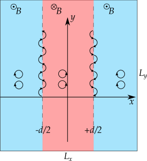
Figure 1: Schematic sketch of the MGW setup viewed from above. A magnetic field $+B\hat{\bm{e}}_{z}$ is applied everywhere in the graphene plane except for the waveguide region $|x|<d/2$, where the field is reversed. Near the field switching lines, quantum modes corresponding to classical snake orbits are realized, while only Landau-quantized cyclotron orbits are present far away from these lines. Several classical orbits corresponding to $n=1$ are schematically illustrated. The system dimensions are $L_{x}$ and $L_{y}$, respectively.

Our MGW setup is illustrated in Fig. 1, where a clean graphene monolayer is exposed to a static inhomogeneous magnetic field. Very long mean free paths have already been realized in graphene, e.g., by using boron nitride as substrate boron . Low-energy quasiparticles close to the neutrality point then correspond to massless Dirac fermions in two spatial dimensions (2D) rmp1 ; rmp2 . The magnetic field is taken spatially inhomogeneous along, say, the $x$-direction, ${\bm{B}}=B(x)\hat{\bm{e}}_{z}$, where we focus on orbital fields such that only the perpendicular ($z$-)component matters. To be specific, we study the field profile, see Fig. 1,

$$B(x)=B\ {\rm sgn}(|x|-d/2)$$ (1)

describing a MGW of transverse width $d$ where the magnetic field is reversed ($B\to-B$) in the waveguide region defined by $|x|<d/2$. Such inhomogeneous magnetic field profiles allow one to guide Dirac fermions ademarti ; ademarti2 ; peeters ; magnscatt ; ghosh ; kuru , and single-particle spectra of the resulting MGW have been analyzed in detail lambert ; tarun ; hausler2 ; bliokh ; prada . For $d\to 0$, Eq. (1) reduces to the familiar homogeneous field case and one recovers the well-known dispersionless relativistic Landau levels, including a zero mode gusynin ; gusynin2 ; goerbig ; miransky . Importantly, such a zero-energy band (with band index $n=0$) is also present for finite $d$, forming the flat band of interest below, while all other ($n\neq 0$) bands acquire dispersion. In particular, near $x=\pm d/2$, pairs of counterpropagating “snake states” develop lambert ; tarun ; sim ; artur ; shakouri , which are either of electron ($n>0$) or hole $(n<0)$ type. Classical snake orbits forming near zero-field lines are illustrated schematically in Fig. 1. We note that snake states have already been observed experimentally in graphene marcus ; ozyilmaz ; christian , including studies of the ballistic (disorder-free) limit christian .

When the $n=0$ level is partially filled, with all negative-energy states occupied, the noninteracting conductance of the MGW vanishes identically since all $n=0$ current matrix elements are zero. We here demonstrate that, nonetheless, a finite conductance emerges due to inter-band Coulomb interactions (corresponding to Landau level mixing for $d=0$ macdon ). The transport features related to the zero-energy band differ qualitatively from those of finite-energy bands, and thus should be easy to identify experimentally.

For the guidance of the focused reader, we now summarize the content of the following sections before starting with the detailed description of our results. We describe the solution of the single-particle problem in Sec. II.1, where in Landau gauge the problem is homogeneous along the $y$-direction and eigenstates for given band index $n$ are classified by the momentum $k_{y}=k$. Coulomb matrix elements are discussed in Sec. II.2, followed by a study of the theory projected to the zero-mode sector in Sec. III. Employing the Hartree-Fock (HF) approximation, we find that the spatial inhomogeneity of the magnetic field generically leads to dispersion of the HF single-particle energies $\varepsilon_{k}$. The HF ground state represents a filled Fermi sea, where all $n=0$ states with $|k|<k_{F}(\nu)$ are occupied, with the zero-mode filling factor $\nu$. We determine the interaction-induced Fermi momentum $k_{F}(\nu)$, and show that the conductance still vanishes within the zero-mode description. In Sec. IV, the zero-temperature linear conductance, $G$, will be computed from the Kubo formula, taking into account inter-band interactions through a systematic perturbative expansion up to second order. For the zero-energy bands, we find completely different transport properties when compared to finite-energy bands. In the latter case, which has been studied in Ref. hausler2 , $G$ is independent of the band filling and quantized in units of the conductance quantum $G_{0}=e^{2}/h$. Moreover, finite-temperature corrections to this quantized value follow the predictions of TLL theory. In marked contrast to these finite-energy bands, the conductance found for the zero-energy case strongly depends on the filling and is not described by TLL theory. Finally, in Sec. V, we shall put our results into a general context. Some calculational details can be found in the Appendix. Throughout this paper, we focus on the most interesting zero-temperature limit and often employ units with $\hbar=1$.

II Magnetic graphene waveguide model

II.1 Single-particle description

We begin by discussing the single-particle description of the MGW, see also Refs. lambert ; tarun . The electronic low-energy physics in a weakly doped graphene monolayer is well described by massless 2D Dirac fermions rmp1 . Including the vector potential ${\bm{A}}$ encoding a static inhomogeneous orbital magnetic field, where only the field component perpendicular to the layer matters, ${\bm{B}}=B(x)\hat{\bm{e}}_{z}$, the single-particle Hamiltonian is given by

$$H_{0}=v_{F}{\bm{\sigma}}\cdot\left(-i{\bm{\nabla}}+\frac{e}{c}{\bm{A}}\right),$$ (2)

where $v_{F}\approx 10^{6}$ m$/$s is the Fermi velocity, ${\bm{\sigma}}=(\sigma_{x},\sigma_{y})$ contains $2\times 2$ Pauli matrices, and ${\bm{\nabla}}=(\partial_{x},\partial_{y})$. The Pauli matrices act in the sublattice space corresponding to the two carbon atoms in the basis of graphene’s honeycomb lattice. The lengthscale on which $B(x)$ changes is assumed large against the lattice spacing ($2.46$ Å), such that valley ($K$ point) mixing is irrelevant. The inclusion of spin and/or valley degrees of freedom is left to future work, although this step is not expected to significantly affect any of our conclusions. As a consequence, we neglect the spin and valley degrees of freedom in Eq. (2) and focus on a single Dirac cone.

We consider the magnetic field profile in Eq. (1), describing a MGW of width $d$, with constant field $B(x)=B$ everywhere except in the strip $|x|<d/2$ where $B\to-B$, see Fig. 1. Using the Landau gauge, the vector potential is given by

$${\bm{A}}=A(x)\hat{\bm{e}}_{y},\quad A(x)=B\times\left\{\begin{array}[]{cc}x+d,&x<-d/2,\\ -x,&|x|<d/2,\\ x-d,&x>d/2.\end{array}\right.$$ (3)

The specific form in Eq. (1) has been adopted in order to keep the discussion focused and to allow for analytical progress. However, other field profiles creating such a MGW are expected to yield similar results tarun , and indeed it is not necessary (nor even desirable) to have atomically sharp changes in the magnetic field profile.

Below we often measure lengths (energies) in units of the magnetic length $l_{B}$ (magnetic energy $E_{B}$),

$$l_{B}=\sqrt{\hbar c/eB},\quad E_{B}=\hbar v_{F}/l_{B}.$$ (4)

We mention in passing that instead of a true magnetic field, one could also employ strain-induced pseudo-magnetic fields strain ; haas , and with minor modifications, similar physics can also be realized by employing the surface states of 3D topological insulators hasan ; rosch .

Periodic boundary conditions along the $y$-direction quantize the conserved momentum $k=k_{y}$ along the MGW. Spinor eigenstates, $\Psi_{n,k}(x,y)$, solving the Dirac equation,

$$H_{0}\Psi_{n,k}=E_{n,k}\Psi_{n,k},$$ (5)

with eigenenergy $E_{n,k}$ can thus be classified by $k$ and the integer band index $n$. For a homogeneous field ($d=0$), Eqs. (2) and (5) lead to the well-known $k$-independent relativistic Landau levels rmp1 ; gusynin ; gusynin2 ; goerbig ; miransky , $E_{n,k}^{(d=0)}={\rm sgn}(n)\sqrt{2|n|},$ and $n$ can be identified with the Landau level index. When $d$ is finite, single-particle states in general exhibit dispersion, but bands with different band index $n$ remain always separated by a finite gap lambert ; tarun . Moreover, even in this inhomogeneous case, a flat zero-energy band is present, $E_{n=0,k}=0$. In this work, we study whether this zero-mode band can carry electric current when Coulomb interaction effects are taken into account.

Owing to momentum conservation along the $y$-direction, we have

$$\Psi_{n,k}(x,y)=\frac{e^{iky}}{\sqrt{L_{y}}}\psi_{n,k}(x),\quad\psi_{n,k}(x)=\left(\begin{array}[]{c}\phi_{n,k}(x)\\ i\chi_{n,k}(x)\end{array}\right),$$ (6)

with the normalization condition $\int dx(\phi^{2}_{n,k}+\chi^{2}_{n,k})=1$. As shown in App. A, both $\phi_{n,k}$ and $\chi_{n,k}$ can be chosen real-valued, and the single-particle problem is solved by matching the respective spinor solutions in the three regions in Fig. 1 at $x=\pm d/2$. The solutions have the symmetry properties

$$\psi_{n,k}(x) = \sigma_{z}\psi_{-n,k}(x)\quad(n\neq 0),$$ (7)

$$\psi_{n,k}(x) = (-1)^{n+1}\psi^{\ast}_{n,-k}(-x),$$

where “$\ast$” indicates complex conjugation of both spinor entries. The first relation says that a particle-hole transformation connects states with $n$ and $-n$ (for $n\neq 0$), and thus the single-particle spectrum is mirror-symmetric around zero energy, $E_{-n,k}=-E_{n,k}$. The second relation follows from inversion symmetry together with the node rule in 1D. Moreover, the matrix elements of the current $I$ (evaluated at $y=0$) along the waveguide ($y$-)direction are given by

$$I_{n,k;n^{\prime}k^{\prime}}=v_{F}\int dx\ \psi_{n,k}^{\dagger}(x)\sigma_{y}\psi_{n^{\prime},k^{\prime}}(x),$$ (8)

where the dagger denotes transposition and complex conjugation of spinor wave functions footcurr . As a consequence of Eq. (7), they satisfy the symmetry relations

$$I_{n,k;-n,k^{\prime}} = -I_{n,k^{\prime};-n,k},$$ (9)

$$I_{0,k;n,k^{\prime}} = (-1)^{n+1}I_{0,-k;n,-k^{\prime}},$$

with arbitrary integer $n$.

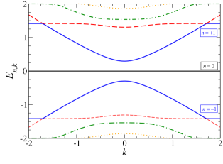
Figure 2: Dispersion relation of the MGW for $d=2l_{B}$. Only the marked three bands ($n=-1,0,1$) will be kept later on in Sec. IV.3, assuming that the zero mode is partially filled. We note that the $n=1$ and $n=2$ bands are separated by an avoided crossing not apparent on the shown scale. Energy (momentum) is given in units of $E_{B}$ ($l_{B}^{-1}$), see Eq. (4).

We next describe the spectrum and the eigenstates for the MGW, where the dispersion relation is shown in Fig. 2 for $d=2l_{B}$. As described in App. A, the spectrum and the eigenstates follow by numerical solution of an eigenvalue problem. However, analytical progress is possible for the zero modes. Indeed, as dictated by index theorems goerbig ; miransky , there must be zero-energy states, $E_{n=0,k}=0$, also for finite $d$, cf. Fig. 2. Using units with $l_{B}=1$, their analytical form is given by

$$\psi_{0,k}(x) = \left(\begin{array}[]{c}0\\ i\chi_{0,k}(x)\end{array}\right),$$ (12)

$$\chi_{0,k}(x) = \frac{e^{d|x|-(x+k)^{2}/2}}{N_{0,k}}\times\left\{\begin{array}[]{cc}1,&|x|>d/2,\\ e^{(|x|-d/2)^{2}},&|x|<d/2,\end{array}\right.$$ (15)

with normalization constant $N_{0,k}$. Due to the absence of an upper spinor component, all zero-mode current matrix elements vanish identically,

$$I_{0,k;0,k^{\prime}}=0.$$ (16)

For $d=0$, the $\chi_{0,k}(x)$ functions reduce to shifted harmonic oscillator ground-state wavefunctions describing the $n=0$ Landau level. For $d\neq 0$, the probability density distribution, $|\psi_{0,k}(x)|^{2}$, has two local maxima near (for $|k|\lesssim d/l_{B}^{2}$) but never inside the waveguide region. For later use, we also mention that a local minimum of $|\psi_{0,k}(x)|^{2}$ exists at $x=kl_{B}^{2}$ when $|k|<d/2l_{B}^{2}$.

Since the $n\neq 0$ (and particularly the $n=\pm 1$) snake states exhibit their probability density maximum near the null lines of the magnetic field tarun at $x=\pm d/2$, cf. Fig. 1, interaction-induced transitions between $n=0$ and $n\neq 0$ states are therefore only important for $|k|\lesssim d/l_{B}^{2}$. The zero-mode conductance $G$ discussed in Sec. IV is caused by precisely such transitions. In fact, as long as virtual band transitions to $n\neq 0$ states are excluded, $G=0$ holds on general grounds since interactions cannot generate an upper spinor component in Eq. (12) from the zero-mode sector only, cf. Eq. (16).

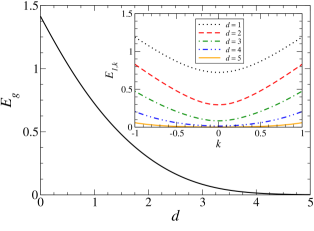
Figure 3: Main panel: Single-particle gap $E_{g}$ vs waveguide width $d$ in units as in Fig. 2. Inset: Long-wavelength part of the dispersion relation for $n=1$ and several values of $d$.

Our perturbative approach in Sec. IV holds as long as the single-particle gap, $E_{g}=E_{n=1,k=0}$, which separates the zero mode from the $n=1$ band, is large against the typical Coulomb energy scale (see Sec. II.2). Figure 3 shows $E_{g}$ as a function of the MGW width $d$. The observed decrease suggests to subsequently consider only $d\lesssim 2l_{B}$. Nonetheless, as shown in App. B, it is also instructive to discuss the limit $d\to\infty$, where a rapid (approximately exponential) decrease of $E_{g}$ is seen in Fig. 3.

II.2 Coulomb interactions

Next we turn to a second-quantized description and include Coulomb interaction effects. The fermion annihilation field operator at ${\bm{r}}=(x,y)$ is written as

$$\hat{\Psi}({\bm{r}})=\sum_{n,k}\Psi_{n,k}({\bm{r}})\ c_{n,k},$$ (17)

with fermion operators $c_{n,k}$ subject to the standard anticommutator algebra, $\{c_{n,k},c_{n^{\prime},k^{\prime}}^{\dagger}\}=\delta_{nn^{\prime}}\delta_{kk^{\prime}}$ and so on, and $\Psi_{n,k}$ in Eqs. (5) and (6). Using the units in Eq. (4), the second-quantized interaction Hamiltonian is given by

$$\hat{H}_{I}=\frac{1}{2}\int d{\bm{r}}d{\bm{r}}^{\prime}\ V({\bm{r}}-{\bm{r}}^{\prime})\hat{\Psi}^{\dagger}({\bm{r}})\hat{\Psi}^{\dagger}({\bm{r}}^{\prime})\hat{\Psi}({\bm{r}}^{\prime})\hat{\Psi}({\bm{r}}),$$ (18)

where we consider a gate-screened Coulomb potential,

$$V({\bm{r}})=\alpha\left(\frac{1}{|{\bm{r}}|}-\frac{1}{\sqrt{|{\bm{r}}|^{2}+4R^{2}}}\right).$$ (19)

Here $\alpha$ denotes graphene’s effective fine structure constant, with typical values in the range $\alpha\approx 0.1$ to $2$, depending on the dielectric properties of the surroundings rmp1 ; rmp2 . The second (image charge) term in Eq. (19) comes from a parallel metallic plate, e.g., due to a gate electrode, at distance $R$ from the graphene layer. The Fourier transform of Eq. (19) is given by (we remind the reader that $k=k_{y}$)

$$\tilde{V}(k_{x},k)=2\pi\alpha\frac{1-e^{-2R\sqrt{k_{x}^{2}+k^{2}}}}{\sqrt{k_{x}^{2}+k^{2}}}.$$ (20)

Inserting Eq. (17) into Eq. (18) and exploiting momentum conservation along the $y$-direction, we obtain

$$\hat{H}_{I} = \frac{1}{2}\sum_{n_{1},n_{2},n_{3},n_{4}}\sum_{k,k^{\prime},q}V_{k,k^{\prime};q}^{(n_{1},n_{2},n_{3},n_{4})}$$ (21)

$$\times c^{\dagger}_{n_{1},k}c^{\dagger}_{n_{2},k^{\prime}}c_{n_{3},k^{\prime}-q}c_{n_{4},k+q},$$

where the Coulomb matrix elements

$$V^{(\{n_{j}\})}_{k,k^{\prime};q}=\frac{1}{L_{y}}\int\frac{dk_{x}}{2\pi}\tilde{V}(k_{x},q){\cal F}^{(n_{1},n_{4})}_{k,q}(k_{x}){\cal F}^{(n_{2},n_{3})}_{k^{\prime},-q}(-k_{x})$$ (22)

are expressed in terms of form factors,

$${\cal F}_{k,q}^{(n,n^{\prime})}(k_{x})=\int dx\ e^{-ik_{x}x}\psi^{\dagger}_{n,k}(x)\cdot\psi_{n^{\prime},k+q}(x).$$ (23)

We show in App. C that the Coulomb matrix elements in Eq. (22) are real-valued and subject to the symmetry relations

$$V^{(n_{1},n_{2},n_{3},n_{4})}_{k,k^{\prime};q} = V^{(n_{2},n_{1},n_{4},n_{3})}_{k^{\prime},k;-q}$$

$$= V^{(n_{4},n_{3},n_{2},n_{1})}_{k+q,k^{\prime}-q;-q}$$

$$= (-1)^{n_{1}+n_{2}+n_{3}+n_{4}}V^{(n_{1},n_{2},n_{3},n_{4})}_{-k,-k^{\prime};-q}.$$

In order to obtain numerical values for the Coulomb matrix elements, we first compute the form factors in Eq. (23) by numerical integration over $x$, taking into account their symmetry properties. Given the form factors, the remaining $k_{x}$-integration in Eq. (22) can then be evaluated numerically in an efficient manner.

Notably, the zero-mode ($n=n^{\prime}=0$) form factors can be evaluated analytically,

$${\cal F}^{(0,0)}_{k,q}(k_{x})=\frac{Y\left(k+\frac{q+ik_{x}}{2}\right)}{\sqrt{Y(k)Y(k+q)}}.$$ (25)

Using again units with $l_{B}=1$, we here use the complex-valued auxiliary function

$$Y(z) = \sum_{\pm}\Bigl{(}e^{(z\mp d)^{2}}{\rm erfc}\left(\pm[z\mp d/2]\right)$$

$$\pm ie^{-z^{2}+d^{2}/2}{\rm erfc}\left(-i[z\mp d/2]\right)\Bigr{)},$$

with the complementary error function ${\rm erfc}(z)$ gradst ; abramowitz . For real-valued argument $z$, the function $Y(z)$ is real and positive. In Sec. III, we shall also refer to the homogeneous case $d\to 0$, where Eq. (II.2) simplifies to $Y(z)\to 2e^{z^{2}}$. The form factors in Eq. (25) then become ${\cal F}^{(0,0)}_{k,q}(k_{x})\to e^{-(k_{x}^{2}+q^{2})/4}e^{i(k+q/2)k_{x}}$, resulting in the zero-mode Coulomb matrix elements

$$\left.V_{k,k^{\prime};q}^{(0,0,0,0)}\right|_{d\to 0} \to \frac{2\alpha}{L_{y}}\Bigl{[}K_{0}\left(|q(k-k^{\prime}+q)|\right)$$

$$- K_{0}\left(|q|\sqrt{4R^{2}+(k-k^{\prime}+q)^{2}}\right)\Bigr{]}$$

with the modified Bessel function $K_{0}$ gradst .

Finally, it simplifies our subsequent analysis to use antisymmetrized Coulomb matrix elements throughout the remainder of this paper,

$$W_{k,k^{\prime};q}^{(n_{1},n_{2},n_{3},n_{4})}=\frac{1}{2}\left(V^{(n_{1},n_{2},n_{3},n_{4})}_{k,k^{\prime};q}-V^{(n_{2},n_{1},n_{3},n_{4})}_{k^{\prime},k;q+k-k^{\prime}}\right),$$ (28)

which follow from Eq. (22) by antisymmetrization under the exchange $(n_{1},k)\leftrightarrow(n_{2},k^{\prime})$. This antisymmetrization simply reflects the fermionic anticommutator algebra. The matrix elements in Eq. (28) are also real-valued and enjoy the same symmetry relations, see Eq. (II.2), as the $V^{(n_{1},n_{2},n_{3},n_{4})}_{k,k^{\prime};q}$.

III Zero mode sector: Hartree-Fock theory

We now consider the case of a partially filled zero mode, where all negative-energy bands ($n<0$) are occupied while all positive-energy states $(n>0)$ are unoccupied. The $n=0$ level has the filling factor $\nu=N/N_{s}$, where $N$ particles occupy the $n=0$ band and the degeneracy degree, $N_{s}$, is given by the total magnetic flux in units of the flux quantum,

$$N_{s}=\frac{(L_{x}-2d)L_{y}}{2\pi l_{B}^{2}},$$ (29)

assuming a rectangular sample, see Fig. 1. The momentum $k=k_{y}$ takes the values $k=2\pi n_{y}/L_{y}$ with $-N_{s}/2<n_{y}\leq N_{s}/2$. This assumption of fully occupied (empty) bands with negative (positive) energy also holds for the interacting ground state as long as the typical Coulomb energy scale is small compared to the single-particle gap $E_{g}$, see Fig. 3. In this section, we consider the zero-mode sector only and thus neglect all Coulomb interaction processes involving $n\neq 0$ states.

In the zero-mode theory, there is no kinetic energy term and the Hamiltonian equals $\hat{H}_{I}$ in Eq. (21), with all $n_{j}=0$ and the form factors in Eq. (25). Unfortunately, numerically exact solutions for this interacting problem are already out of reach except for very small system size. Here we instead proceed by employing the textbook Hartree-Fock (HF) approximation hftextbook . However, going beyond this approximation is expected to cause at most quantitative – but not qualitative – modifications of the interaction-induced conductance discussed later on. Note also that for the corresponding homogeneous ($d\to 0$) problem, HF calculations give a good understanding of the physics away from rational filling factors related to the fractional quantum Hall effect rmp1 ; rmp2 ; nomura ; moessner ; joglekar ; cote ; christiane ; faugeras . As HF parameters we choose the occupation numbers

$$n_{k}=\left\langle c_{0,k}^{\dagger}c_{0,k}\right\rangle,$$ (30)

where the expectation value is self-consistently taken with respect to the HF approximation of the zero-mode Hamiltonian. For given filling factor $\nu$, the HF parameters have to be determined under the condition $\sum_{k}n_{k}=N=\nu N_{s}.$ By choosing the $n_{k}$ as HF parameters, we disregard the possibility of charge density wave or Wigner crystal formation hftextbook . Note that Wigner crystallization was reported in the homogeneous case ($d=0$) with unscreened ($R\to\infty$) Coulomb interactions for certain filling factors $\nu$ joglekar ; cote ; christiane . However, for our MGW with externally screened interactions, see Eq. (19), we do not expect such phases.

Defining single-particle energies as

$$\varepsilon_{k}=\sum_{k^{\prime}}W_{k,k^{\prime}}n_{k^{\prime}},\quad W_{k,k^{\prime}}=2W^{(0,0,0,0)}_{k,k^{\prime};q=0},$$ (31)

with the Coulomb matrix elements in Eq. (28), the HF estimate for the ground-state energy reads

$${\cal E}^{\rm HF}_{0}=\frac{1}{2}\sum_{k}\varepsilon_{k}n_{k}.$$ (32)

The HF iteration starts with a normalized random initial distribution for $n_{k}$, where we assume $n_{-k}=n_{k}$. Next the HF energies $\varepsilon_{k}$ in Eq. (31) are computed, where $\varepsilon_{-k}=\varepsilon_{k}$ by virtue of the symmetry relations (II.2). The updated distribution $n_{k}$, which is obtained by occupying the $N$ energetically lowest states, therefore always remains even in $k$. The scheme is then iterated until convergence has been reached.

We find that the HF ground-state energy converges quickly from above. However, there are many local energy minima in occupation number space, and depending on the initial configuration one may converge to states of widely different energy. We obtain the global minimum by comparing converged results for sufficiently many (typically a few hundred) randomly chosen initial states. The smooth behavior of all calculated quantities, such as the ground-state energy or the effective Fermi momentum, on the system parameters also confirms that this procedure reliably finds the HF ground state. For the results shown here, graphene’s fine structure constant [see Eq. (19)] was taken as $\alpha=0.5$, with the MGW width $d=2l_{B}$ as in Fig. 2. To check our conclusions, we have performed additional calculations for other parameters, where the results (not shown) confirm the physical picture presented in what follows.

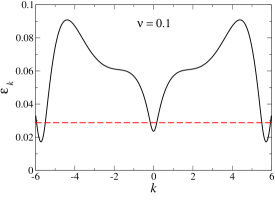
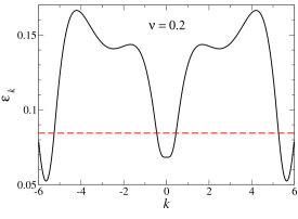
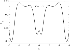
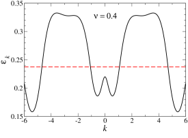
Figure 4: Self-consistent zero-mode HF energies $\varepsilon_{k}$ (in units of $E_{B}$) for various filling factors $\nu$. The red dashed horizontal lines denote the chemical potential at the respective filling, with all lower states occupied. We consider $\alpha=0.5$, $d=2l_{B}$, $R=d$, $L_{x}=16l_{B}$, and $N_{s}=400$ basis states, see Eq. (29). This parameter set corresponds to $L_{y}=209.4\leavevmode\nobreak\ l_{B}$, where $|k|=\pi N_{s}/L_{y}=6l_{B}^{-1}$ represents the zone boundary.

The zero-mode HF dispersion relation is shown in Fig. 4. For all studied filling factors, we found that the HF energies $\varepsilon_{k}$ develop a pronounced dip for small momenta, corresponding to states located mainly within the waveguide region, $|k|\lesssim d/l_{B}^{2}$. For larger $|k|$, we instead expect an almost flat dispersion (see below). However, Fig. 4 reveals a preferential population of states at large momenta, which are spatially localized near the boundaries at $x=\pm L_{x}/2$. To understand this feature, it is instructive to briefly study the homogeneous field case, $d\to 0$. Using Eqs. (II.2) and (31), we observe that for a $k$-independent distribution, $n_{k}=\nu$, the HF energies (31) are given by $\varepsilon_{k}\simeq(\nu L_{y}/2\pi)\int_{-L_{x}/2}^{L_{x}/2}dk^{\prime}W_{k,k^{\prime}}$. Ignoring boundary effects, one could then effectively shift the integration variable $k^{\prime}$ to absorb $k$, resulting in $k$-independent energies $\varepsilon_{k}$. However, for states localized near the edge of the sample, dispersion is already predicted by this $d=0$ result. Such “Pauli holes” near the sample edges are clearly observed in Fig. 4. However, these boundary states play no role for the zero-mode conductance $G$, since they have no significant interaction matrix elements with snake states. We can therefore safely ignore large-momentum states. In practice, we keep only single-particle states with $|k|\leq k_{c}$, where the momentum cutoff is chosen as $k_{c}\approx d/l_{B}^{2}$, cf. Sec. IV.3.

For very small filling factor, $\nu\lesssim 0.08$, the $k=0$ minimum in the dispersion is above the Fermi level such that no small-$k$ modes are occupied. At larger fillings, however, Fig. 4 shows that this minimum in $\varepsilon_{k}$ drops below the Fermi level, and then evolves into a double minimum with increasing $\nu$. The latter feature can be understood from the reduced probability density $|\psi_{0,k}(x)|^{2}$ inside the waveguide region. This density has a local minimum at $x=kl_{B}^{2}$ (for $|k|<d/2l_{B}^{2}$) and thus comes with a reduced Coulomb repulsion cost. Finally, for $\nu\gtrsim 0.5$, we find that the HF energies may exceed the single-particle gap, $\varepsilon_{k}>E_{g}$. Since in that case our assumption of well-separated bands may break down, we shall focus on the window $0.1\lesssim\nu\lesssim 0.4$ in what follows. Within this window, the perturbative approach in Sec. IV is justified.

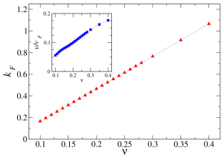
Figure 5: Interaction-induced Fermi momentum $k_{F}$ vs filling factor $\nu$ for the parameters in Fig. 4. The dotted curve is a guide to the eye only. Note the approximately linear $\nu$-dependence. The inset shows the effective Fermi velocity $v$ vs $\nu$, where $v$ is given in units of graphene’s Fermi velocity $v_{F}$.

The respective Fermi level then intersects $\varepsilon_{k}$ for $k=\pm k_{F}$ with $k_{F}\lesssim d$. The effective Fermi momentum, $k_{F}(\nu)$, and effective Fermi velocity, $v(\nu)$, are depicted as a function of the filling factor in Fig. 5, where $v$ was obtained by linearizing $\varepsilon_{k}$ around $k=k_{F}$. It is worth mentioning that while the results in Figs. 4 and 5 were obtained for $\alpha=\alpha_{0}=0.5$, the corresponding results for $\alpha\neq\alpha_{0}$ follow from a simple scaling argument. In particular, while $k_{F}$ is independent of $\alpha$, we find $\varepsilon_{k}^{(\alpha)}=(\alpha/\alpha_{0})\varepsilon_{k}^{(\alpha_{0})}$ and thus $v^{(\alpha)}=(\alpha/\alpha_{0})v^{(\alpha_{0})}$.

The converged HF results for $\varepsilon_{k}$ can tentatively be interpreted as signature for an interaction-induced single-particle dispersion, where the low-energy physics is governed by a single pair of right- and left-movers with nearly linear dispersion relation and well-defined Fermi momentum. Nonetheless, the conductance remains zero unless we also include virtual band transitions to $n\neq 0$ states. This statement holds true even under an exact treatment of interactions (beyond HF theory), since no upper spinor components in Eq. (12) and thus no finite current matrix elements can then be generated.

IV Conductance

In this section, we study the zero-temperature linear DC-conductance, $G$, of the MGW when the $n=0$ band is partially filled. Within the HF approach in Sec. III, intra-band $n=0$ Coulomb interactions were shown to be responsible for an effective Fermi momentum $k_{F}=k_{F}(\nu)$, where $\nu$ is the filling factor, such that all single-particle states below the Fermi energy $E_{F}=\varepsilon_{k_{F}}$ are occupied. We here address the question: Are Coulomb interactions able to induce a finite conductance in the clean system? Anticipating the affirmative answer to this question, this feature offers a powerful novel way to directly probe electron-electron interaction effects in clean graphene samples through transport measurements.

IV.1 Kubo formula

We follow the standard Kubo linear-response formalism altland , expressing the linear conductance as

$$G=-e^{2}\lim_{\omega\to 0}\frac{{\rm Im}\Pi^{R}(\omega)}{\omega},$$ (33)

where $\Pi^{R}(\omega)$ is the Fourier transform of the retarded current-current correlation function,

$$\Pi^{R}(t)=-i\Theta(t)C(t),\quad C(t)=\langle\Phi|[\hat{I}(t),\hat{I}(0)]_{-}|\Phi\rangle,$$ (34)

with $\hat{I}(t)=e^{iHt}\hat{I}e^{-iHt}$, the Heaviside step function $\Theta(t)$, and the normalized ground state $|\Phi\rangle$ of the full Hamiltonian $H$. In second-quantized notation, the particle current along the $y$-direction is described by the operator

$$\hat{I}=\sum_{n,n^{\prime}}\sum_{k,k^{\prime}}I_{n,k;n^{\prime},k^{\prime}}c_{n,k}^{\dagger}c_{n^{\prime},k^{\prime}},$$ (35)

with the matrix elements in Eq. (8). Following a sequence of standard steps, the Fourier transform, $\tilde{C}(\omega)$, of the current-current correlator, $C(t)$, is related to the imaginary part of $\Pi^{R}(\omega)$, and thus represents a spectral function for current fluctuations. Indeed, noting that $C^{*}(-t)=C(t)$ implies real-valuedness of $\tilde{C}(\omega)$, we find ${\rm Im}\Pi^{R}(\omega)=-\tilde{C}(\omega)/2$. Furthermore, we note that $\tilde{C}(0)=0$ because of $C(-t)=-C(t)$. The conductance thus follows as

$$G=\pi G_{0}\frac{d\tilde{C}}{d\omega}(\omega=0),$$ (36)

where $G_{0}=e^{2}/h$ is the conductance quantum. Writing $C(t)=X(t)-X(-t)$, we then need to evaluate the correlation function

$$X(t)=\langle\Phi|\hat{I}(t)\hat{I}(0)|\Phi\rangle.$$ (37)

At this point, it is useful to write the full Hamiltonian as $H=\hat{H}_{0}+\hat{W}$, where $\hat{H}_{0}$ captures not only the noninteracting part, cf. Eq. (2), but also includes the $n=0$ HF Coulomb interaction terms discussed in Sec. III. Writing $\hat{H}_{0}=\sum_{n,k}\tilde{E}_{n,k}c_{n,k}^{\dagger}c_{n,k},$ with the effective single-particle energies $\tilde{E}_{n\neq 0,k}=E_{n,k}$ and $\tilde{E}_{0,k}=\varepsilon_{k}$, all remaining interactions processes are then encoded by $\hat{W}$, which in particular describes inter-band transitions. For $\hat{W}=0$, the ground state $|\Phi\rangle=|\Phi_{0}\rangle$ corresponds to a Fermi sea with the occupation numbers

$$f_{n,k}=f(\tilde{E}_{n,k}),\quad f(E)=\Theta(E_{F}-E),$$ (38)

where $f(E)$ is the Fermi function taken, for simplicity, at zero temperature.

In order to include $\hat{W}$, it is convenient to evaluate $X(t)$ in Eq. (37) by using the Keldysh Green’s function technique, where the time evolution proceeds from $t=-\infty$ to $t=+\infty$ (forward branch, $s=+$) and back from $t=+\infty$ to $t=-\infty$ (backward branch, $s=-$) altland . From now on, we use the interaction picture, where time-dependent operators are denoted by $\hat{I}(t)=e^{it\hat{H}_{0}}\hat{I}e^{-it\hat{H}_{0}}$. We then have to double all dynamical fields according to the branch $s=\pm$ of the Keldysh contour, $\hat{I}(t)\to\hat{I}_{s}(t)$ and so on. As a result, $X(t)$ takes the form

$$X(t)=\left\langle\Phi_{0}\left|{\cal T}_{C}\left[S(\infty)\hat{I}_{-}(t)\hat{I}_{+}(0)\right]\right|\Phi_{0}\right\rangle,$$ (39)

where ${\cal T}_{C}$ is the time-ordering operator along the Keldysh contour, and the time-evolution operator reads

$$S(\infty)={\cal T}_{C}\exp\left(-i\int_{-\infty}^{\infty}d\tau\sum_{s=\pm}s\hat{W}_{s}(\tau)\right).$$ (40)

IV.2 Diagrammatic expansion

Our strategy will be to compute the conductance as perturbation series in the interaction term $\hat{W}$, which captures the effects of virtual band transitions. Going up to second order in $\hat{W}$ yields

$$G=G^{(0)}+G^{(1)}+G^{(2)}+O(\hat{W}^{3}).$$ (41)

Expanding Eq. (40) in powers of $\hat{W}$, we obtain a corresponding series for $X(t)=X^{(0)}+X^{(1)}+X^{(2)}+\cdots$, with the $m$-th order term given by

$$X^{(m)}(t)=\frac{(-i)^{m}}{m!}\int_{-\infty}^{\infty}d\tau_{1}\cdots d\tau_{m}\sum_{s_{1},\ldots,s_{m}=\pm}s_{1}\cdots s_{m}$$

$$\times\left\langle\Phi_{0}\left|{\cal T}_{C}\left[\hat{W}_{s_{1}}(\tau_{1})\cdots\hat{W}_{s_{m}}(\tau_{m})\hat{I}_{-}(t)\hat{I}_{+}(0)\right]\right|\Phi_{0}\right\rangle.$$ (42)

Application of Wick’s theorem to the time-ordered products of noninteracting fermion operators in Eq. (42) allows one to interpret such expressions in a diagrammatic language. The propagator (“line”) in a given diagram then corresponds to the Keldysh Green’s function (with Keldysh indices $s,s^{\prime}=\pm$) altland ,

$${\cal G}^{(s,s^{\prime})}_{n,k}(t-t^{\prime})=-i\langle\Phi_{0}|{\cal T}_{C}[c_{n,k,s}(t)c^{\dagger}_{n,k,s^{\prime}}(t^{\prime})]|\Phi_{0}\rangle,$$ (43)

with the Fourier-transformed components

$$\tilde{\cal G}_{n,k}^{(s,s)}(E) = \frac{s}{E-\tilde{E}_{n,k}+is\ {\rm sgn}\left(\tilde{E}_{n,k}-E_{F}\right)\ 0^{+}},$$

$$\tilde{\cal G}_{n,k}^{(s,-s)}(E) = 2\pi isf(sE)\ \delta\left(E-\tilde{E}_{n,k}\right),$$ (44)

where $f(E)$ is the Fermi function, see Eq. (38). All conductance diagrams up to order $m=2$ are shown in Figs. 6 and 7. They are constructed from the following rules:

• Each diagram must contain two external (two-point) vertices representing the current operators $\hat{I}_{-}(t)$ and $\hat{I}_{+}(0)$. These vertices carry the respective Keldysh index $s=\pm$, and are denoted by filled circles in Figs. 6 and 7.

• For an $m$-th order diagram, there are $m$ internal (four-point) vertices representing the interaction Hamiltonian, i.e., factors $s\hat{W}_{s}(\tau)$. These vertices are denoted by filled squares.

• Using the Keldysh normalization condition $\langle\Phi_{0}|S(\infty)|\Phi_{0}\rangle=1$ as well as $\langle\Phi|\hat{I}_{\pm}(t)|\Phi\rangle=0$, only connected diagrams have to be taken into account.

We mention in passing that in evaluating low-order diagrams it is useful to exploit a “selection rule” that allows one to discard certain contributions without detailed calculation. Indeed, owing to the vanishing current matrix elements in Eq. (16), a diagrammatic contribution is zero whenever a current vertex with Keldysh index $s=\pm$ is connected to two other vertices that both have the opposite Keldysh index $-s$ foot .

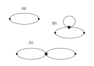
Figure 6: Diagrammatic expansion of the conductance (see main text). Panel (a) shows the zeroth-order ($m=0$) diagram, while (b) and (c) refer to the two first-order ($m=1$) diagrams.

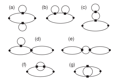
Figure 7: Same as Fig. 6 but for the second-order ($m=2$) diagrams.

At this stage, it is convenient to introduce several auxiliary matrices. First, we define the current matrix $I$ through its matrix elements $I_{n,k;n^{\prime},k^{\prime}}$ in Eq. (8). Second, the hybridization matrix $\Lambda$ with

$$\Lambda_{n,k;n^{\prime},k^{\prime}}=\frac{\delta_{k,k^{\prime}}(1-\delta_{n,n^{\prime}})}{\tilde{E}_{n,k}-\tilde{E}_{n^{\prime},k}}\sum_{n_{1},k_{1}}f_{n_{1},k_{1}}W_{k,k_{1};q=0}^{(n,n_{1},n_{1},n^{\prime})}$$ (45)

describes interaction-induced virtual transitions between different bands. Here the intermediate summation comes from a fermion loop. We notice that $\Lambda$ is diagonal in $k$-space and hence can indeed be interpreted as hybridization matrix. The commutator of the above matrices is given by

$$\delta I=[I,\Lambda]_{-},$$ (46)

which captures the current matrix renormalization by virtual interband transitions to leading order. Finally, we introduce a fluctuation matrix $K$, with matrix elements

$$K_{n,k;n^{\prime}k^{\prime}} = \sum_{n_{1},k_{1};n_{2},k_{2}}\delta_{k_{2},k_{1}+k^{\prime}-k}\frac{f_{n_{1},k_{1}}-f_{n_{2},k_{2}}}{\tilde{E}_{n_{2},k_{2}}-\tilde{E}_{n_{1},k_{1}}}$$ (47)

$$\times I_{n_{1},k_{1};n_{2},k_{2}}W^{(n_{2},n,n_{1},n^{\prime})}_{k_{2},k;k-k_{1}}.$$

Below, the “$\circ$” symbol denotes Fermi level convolution, i.e., the matrix elements of $A\circ B$ are given by

$$(A\circ B)_{n,k;n^{\prime},k^{\prime}}=\sum_{\pm}A_{n,k;0,\pm k_{F}}B_{0,\pm k_{F};n^{\prime},k^{\prime}},$$ (48)

and “Tr_F” denotes a Fermi level trace,

$${\rm Tr}_{F}A=\sum_{\pm}A_{0,\pm k_{F};0,\pm k_{F}}.$$ (49)

Let us now start with the zeroth-order conductance contribution, where inter-band transitions are absent. From the discussion in Sec. III, this term is expected to vanish identically, $G^{(0)}=0$. There is only a single $m=0$ diagram, represented by the polarization bubble in Fig. 6(a). By virtue of Eqs. (42) and (43), this diagram leads to the correlation function

$$X^{(0)}(t)=\sum_{n,k;n^{\prime},k^{\prime}}\left|I_{n,k;n^{\prime},k^{\prime}}\right|^{2}{\cal G}_{n,k}^{(-,+)}(t){\cal G}^{(+,-)}_{n^{\prime},k^{\prime}}(-t).$$ (50)

Performing a Fourier transformation, we find

$$\tilde{X}^{(0)}(\omega) = 2\pi\sum_{n,k;n^{\prime},k^{\prime}}\left|I_{n,k;n^{\prime},k^{\prime}}\right|^{2}$$

$$\times (1-f_{n,k})f_{n^{\prime},k^{\prime}}\delta(\tilde{E}_{n,k}-\tilde{E}_{n^{\prime},k^{\prime}}-\omega),$$

and with Eq. (36), the respective zero-temperature conductance contribution is

$$G^{(0)}/G_{0}=\frac{\pi^{2}\rho_{0}^{2}}{2}\ {\rm Tr}_{F}(I\circ I).$$ (52)

Here $\rho_{0}=1/\pi v$ denotes the density of states, with $v=\partial_{k}\varepsilon_{k=k_{F}}$, and the symbols “$\circ$” and “Tr_F” were defined in Eqs. (48) and (49), respectively. Since all current matrix elements appearing in Eq. (52) vanish by virtue of Eq. (16), this calculation confirms the expected result $G^{(0)}=0$.

Let us then turn to the first-order ($m=1$) diagrams. After some algebra, the corresponding conductance contribution takes the form

$$G^{(1)}/G_{0}=-2\pi^{2}\rho_{0}^{2}\ {\rm Tr}_{F}\left[I\circ(\delta I-K)\right],$$ (53)

where the $\delta I$-term comes from diagram (b) and the $K$-term from diagram (c) in Fig. 6, respectively, see also Eqs. (46) and (47). Because of the vanishing zero-mode current matrix elements in Eq. (16), also this conductance contribution vanishes, $G^{(1)}=0$. However, it is worth mentioning that for a conventional system with non-zero current matrix elements, e.g., the finite-energy bands for our MGW, Eqs. (52) and (53) yield finite results, corresponding to the “noninteracting” conductance and the ballistic version of the “interaction correction” aa ; zala ; kupfer , respectively.

In order to encounter a finite conductance in our zero-mode system, we have to go up to second order ($m=2$). All topologically distinct $m=2$ diagrams are shown in Fig. 7. Using the above selection rule, we find that diagram (c) also gives no conductance contribution. Moreover, diagrams (f) and (g) vanish as well since they involve products of more than two Fermi factors which never satisfy the resulting energy constraints. Within second-order perturbation theory, the conductance is thus obtained from the remaining diagrams in Fig. 7, $G=G^{(2)}=G_{a}+G_{b}+G_{d}+G_{e}$, which yield a finite result. Evaluating diagrams (a) and (b) together gives

$$(G_{a}+G_{b})/G_{0}=2\pi^{2}\rho_{0}^{2}\ {\rm Tr}_{F}(\delta I\circ\delta I).$$ (54)

Similarly, diagram (d) yields

$$G_{d}/G_{0}=-4\pi^{2}\rho_{0}^{2}\ {\rm Tr}_{F}(\delta I\circ K),$$ (55)

while diagram (e) produces the contribution

$$G_{e}/G_{0}=2\pi^{2}\rho_{0}^{2}\ {\rm Tr}_{F}(K\circ K).$$ (56)

Collecting all diagrams, we obtain a manifestly positive and general result for the zero-mode conductance,

$$G/G_{0}=2\pi^{2}\rho_{0}^{2}\ {\rm Tr}_{F}\left[(\delta I-K)\circ(\delta I-K)\right].$$ (57)

We note in passing that Eq. (57) does not apply for $d\to 0$, where the zero-mode dispersion $\varepsilon_{k}$ becomes flat and hence $k_{F}$ is not defined anymore.

IV.3 Zero-mode MGW conductance

We next discuss the zero-mode MGW conductance predicted by Eq. (57), adopting the parameters in Sec. III. Our main goals are (i) to reliably demonstrate the existence of a finite zero-mode conductance, and (ii) to clarify its filling dependence. In order to simplify the numerical evaluation, which is quite cumbersome due to the presence of interaction matrix elements connecting all different bands, we shall here evaluate Eq. (57) by taking into account only the three bands $n=-1,0,1$ sketched in Fig. 2. Indeed, the $n=\pm 1$ bands are energetically closest to the $n=0$ modes and therefore produce the main conductance contribution. Moreover, to avoid spurious finite-size effects, we introduce a momentum bandwidth $k_{c}$ restricting the single-particle Hilbert space to states with $|k|\leq k_{c}$, see Sec. III. For the results below, where $d=2l_{B}$, we chose the momentum cutoff $k_{c}=1.6l_{B}^{-1}$. However, taking other values within the range $1.5\lesssim k_{c}l_{B}\lesssim 1.7$ also gave essentially identical results.

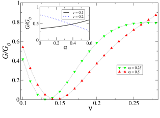
Figure 8: Zero-mode waveguide conductance $G$ (in units of $G_{0}=e^{2}/h$) vs filling $\nu$, see Eq. (57), for two values of the fine structure constant $\alpha$. Dotted curves are guides to the eye only. All other parameters are as in Fig. 4. The inset shows the $\alpha$-dependence at two selected fillings.

The resulting zero-temperature conductance is illustrated in Fig. 8. The main panel shows that the conductance strongly depends on the zero-mode filling factor $\nu$, with a pronounced minimum around $\nu=\nu_{\rm min}$, where we find $\nu_{\rm min}\approx 0.145$ at $\alpha=0.5$. Near this minimum, $G$ becomes very small. The existence of the minimum in $G(\nu)$ can be rationalized by analyzing the Coulomb-assisted hybridization of zero modes with the $n=\pm 1$ bands. For small filling $\nu$, and therefore small chemical potential, see Sec. III, the band $n=-1$ still remains close to the $n=0$ states. In that case, the current renormalization effects encoded in $\delta I$ are found to dominate the conductance in Eq. (57). With increasing filling, this conductance contribution begins to weaken, while the Fermi level gets closer and closer to the $n=1$ band. Eventually, at large filling, the fluctuation matrix $K$ instead dominates in Eq. (57). We then encounter a nearly perfect cancellation of the $\delta I$ and $K$ terms for filling factor $\nu\approx\nu_{\rm min}$.

The inset of Fig. 8 shows the $\alpha$-dependence of the conductance for two fillings $\nu$, chosen below and above $\nu_{\rm min}$, respectively. Two comments are in order here. First, the limit $\alpha\to 0$ seems to result in a finite conductance. This may come as a surprise, since in the absence of interactions, we know that $G=0$ must hold. However, one should keep in mind that our HF approach in Sec. III applies only if the frequency scale $\omega$ at which the conductance is probed remains well below the effective bandwidth of the zero mode. Since this $\varepsilon_{k}$ bandwidth is proportional to $\alpha$, it vanishes in the limit $\alpha\to 0$, and the $\omega\to 0$ limit implicit in Eq. (57) cannot be taken anymore. Second, the different $\alpha$-dependence at the two fillings observed in the inset of Fig. 8 simply reflects the fact that $\nu_{\rm min}$ increases with increasing $\alpha$, cf. the main panel. This shift of $\nu_{\rm min}$ in turn can be rationalized by noting that the chemical potential also moves up with increasing $\alpha$, and thus the cancellation point between the $\delta I$ and $K$ contributions is slightly shifted towards larger fillings.

It is instructive to contrast the above results for the zero-mode conductance with the conductance found when the chemical potential intersects one of the $n\neq 0$ bands instead. This case has been studied in detail in Ref. hausler2 , where a completely different behavior has been reported. When contacted by wide electrodes, the zero-temperature conductance then assumes a quantized value (in units of $G_{0}$), where transport proceeds predominantly through snake states. This quantization can be rationalized by noting that right- and left-moving snake states are spatially separated hausler2 . In addition, no pronounced dependence of the conductance on the respective band filling is expected, in marked contrast to the zero-mode case shown in Fig. 8. As we elaborate further in Sec. V, the finite-energy bands correspond to a realization of the conventional TLL phase, which could also be detected through the predicted power-law corrections to the conductance at finite temperatures hausler2 .

To summarize, the strong dependence of the zero-mode conductance $G(\nu)$ on the filling factor $\nu$, see Fig. 8, should allow for a clear experimental signature of the predicted interaction-induced conducting phase. As we argue in the next section, such a state is distinct from a TLL state, and hence also not described by Fermi liquid theory.

V Discussion

In strictly 1D band metals, it is well known that low-energy excitations near the Fermi points at $\pm k_{F}$ are severely restricted as a consequence of phase-space limitations hftextbook , and therefore any nonzero electron-electron interaction slightly destabilizes the Fermi liquid gogolin-book . The resulting phase is commonly coined “Tomonaga-Luttinger liquid” (TLL), where all low-energy properties of the system are fully determined by just two parameters when disregarding the spin sector haldane ; voit ; giamarchi . If Galilei invariance holds in addition, which is the case for the continuum model considered here, a single TLL parameter, $g_{\rm TLL}$, remains. The Fermi liquid case is recovered for $g_{\rm TLL}=1$. The Kubo conductance of an infinitely long and clean TLL is $G=g_{\rm TLL}G_{0}$ apelrice , and single-particle correlation functions exhibit power-law behavior with exponents controlled by $g_{\rm TLL}$ gogolin-book ; voit . To give just one example, the equal-time single-particle Green’s function, cf. Eq. (17), has the asymptotic power-law decay $\langle\hat{\Psi}(x,y)\hat{\Psi}^{\dagger}(x,0)\rangle\sim|y|^{-\gamma}$ with $\gamma=1+[g_{\rm TLL}+1/g_{\rm TLL}-2]/4$. The value of $g_{\rm TLL}$ is fixed by the interaction strength through the ground-state compressibility voit ,

$$g_{\rm TLL}=\left[\frac{\pi}{v}\frac{\partial^{2}({\cal E}_{0}/L_{y})}{\partial k_{F}^{2}}\right]^{-1/2},$$ (58)

where ${\cal E}_{0}$ is the ground-state energy and $v=|\partial_{k}\varepsilon_{k=k_{F}}|$ the single-particle velocity, see also Ref. kecke . Precisely this scenario has previously been identified in our MGW for all $n\neq 0$ snake states hausler2 . Without interactions, snake states propagate uniformly at the Fermi velocity $v_{F}$ of the graphene host. They represent spatially separated chiral branches located near either of the two parallel zero lines of the magnetic field. The value of $g_{\rm TLL}$ is then governed by Coulomb interactions between these oppositely moving branches and can be tuned directly via the MGW width $d$.

On the other hand, the partially filled $n=0$ MGW band investigated here clearly does not fit into the above TLL framework. First, without interactions there is no Fermi surface, since the zero-energy level is strictly flat. Second, when accounting for intra-band Coulomb interactions on the level of the HF approximation, we found an interaction-induced dispersion, where the effective single-particle energies allow us to define a Fermi momentum, $k_{F}$, and a Fermi velocity, $v$, see Fig. 5. One may then naively conclude that once again a TLL emerges, where $g_{\rm TLL}$ follows from Eqs. (32) and (58). However, this value of $g_{\rm TLL}$ does not describe correctly the conductance of the system which is zero. We stress that the vanishing conductance of the $n=0$ band alone holds true even when performing an exact calculation, see Sec. III. Therefore, contrary to all $n\neq 0$ bands, we conclude that the $n=0$ band cannot be described by a bosonized Gaussian field theory underlying the Luttinger liquid concept haldane . Only when accounting for virtual interband transitions to conducting $n\neq 0$ bands, the $n=0$ band acquires a nonzero conductance for which we find a quite peculiar dependence on the filling $\nu$.

We expect that apart from the MGW studied here, similar behavior should be observable also in other settings. For instance, consider metallic carbon nanotubes with a magnetic field applied perpendicular to the tube axis tcnt . This field should be inhomogeneous on the scale of the tube radius, such that a non-zero net magnetic flux $\Phi$ penetrates the tube, since only then a finite degeneracy, $\Phi/(hc/e)$, of the $n=0$ Landau level is guaranteed by index theorems goerbig , see also Ref. prada . Accounting for intra-Landau level interactions, we expect that dispersion of the $n=0$ level is created. Nonetheless, the system will still exhibit insulating behavior when the Fermi level is close to neutrality, and only when including inter-Landau level interactions, a non-zero conductance can emerge. Similar to the case of the MGW, the actual value of the conductance will then give direct information on the strength of the Coulomb interaction, and the conductance behavior of the $n=0$ level should again significantly differ from all $n\neq 0$ bands.

Our theory assumes that one works with a ballistic (disorder-free) sample. We expect that very weak disorder will not qualitatively change the scenario outlined above, but strong disorder will introduce localization and thereby destroy the physics described here. Since ballistic transport is nowadays reachable in high-quality graphene devices, our results should be testable in the near future.

To conclude, the zero-energy levels in a clean magnetic graphene waveguide are predicted to display qualitatively different conductance features than the bands of nonzero energy. For the latter, the zero-temperature conductance is quantized in multiples of the conductance quantum. In contrast, the zero-mode conductance is non-universal with a strong dependence on the filling factor. Since without Coulomb interactions this conductance vanishes identically, transport experiments offer a direct interaction probe. We hope that our predictions can soon be put to an experimental test and will inspire further studies of this novel transport regime.

Appendix A Spectrum of MGW

In this Appendix, we provide some details concerning Sec. II.1. For given $k$, using the natural units in Eq. (4), $H_{0}$ in Eq. (2) reduces to the 1D Hamiltonian

$$H_{0}^{(k)}=-i\sigma_{x}\partial_{x}+[k+A(x)]\sigma_{y},$$ (59)

where $A(x)$ in Eq. (3) is antisymmetric under $x$-inversion, ${\cal R}_{x}:x\to-x$. Due to this property, $H_{0}^{(k)}$ exhibits inversion symmetry,

$$\left[H^{(k)}_{0},\Xi\right]_{-}=0,\quad\Xi={\cal R}_{k}{\cal R}_{x}{\cal C},$$ (60)

where ${\cal R}_{k}:k\to-k$ inverts $k$ and ${\cal C}$ denotes complex conjugation. The operator $\Xi$ has eigenvalues $\xi=\pm$, and Eq. (60) implies that the eigenstates in Eq. (6) obey the relation

$$\Xi\psi_{n,k}(x)=\psi_{n,-k}^{\ast}(-x)=\pm\psi_{n,k}(x).$$ (61)

Next, we note that for $x<-d/2$, the general solution at energy $E=E_{n,k}$ can be written in the form ademarti

$$\psi_{n,k;I}(x)=C^{(n,k)}_{I}\left(\begin{array}[]{c}D_{-1+E^{2}/2}\left(-\sqrt{2}(x+k+d)\right)\\ -\frac{i\sqrt{2}}{E}D_{E^{2}/2}\left(-\sqrt{2}(x+k+d)\right)\end{array}\right),$$ (62)

with a coefficient $C_{I}^{(n,k)}$ and the parabolic cylinder function $D_{p}(x)$ gradst ; abramowitz . Similarly, with coefficients $C^{(n,k)}_{\pm,II}$, the solution in the waveguide region $|x|<d/2$ reads

$$\psi_{n,k;II}(x)=\sum_{\pm}C^{(n,k)}_{\pm,II}\left(\begin{array}[]{c}D_{E^{2}/2}\left(\pm\sqrt{2}(x-k)\right)\\ \mp\frac{iE}{\sqrt{2}}D_{-1+E^{2}/2}\left(\pm\sqrt{2}(x-k)\right)\end{array}\right),$$ (63)

while for $x>d/2$, one finds

$$\psi_{n,k;III}(x)=C_{III}^{(n,k)}\left(\begin{array}[]{c}D_{-1+E^{2}/2}\left(\sqrt{2}(x+k-d)\right)\\ \frac{i\sqrt{2}}{E}D_{E^{2}/2}\left(\sqrt{2}(x+k-d)\right)\end{array}\right).$$ (64)

The symmetry relations in Eq. (61) now connect the coefficients in Eqs. (62), (63) and (64). With $\xi=\pm$, we find the relations

$$C^{(n,k)}_{I}=\xi\left(C^{(n,-k)}_{III}\right)^{*},\quad C^{(n,k)}_{\pm,II}=\xi\left(C^{(n,-k)}_{\mp,II}\right)^{*}.$$ (65)

Let us then choose the overall phase of each eigenstate such that all $C_{I}^{(n,k)}$ are real-valued. Hence Eq. (65) implies that all coefficients in the vector ${\bm{C}}_{n,k}=\left(C^{(n,k)}_{I},C^{(n,k)}_{+,II},C^{(n,k)}_{-,II},C^{(n,k)}_{III}\right)^{T}$ are also real-valued, which in turn confirms that $\phi_{n,k}$ and $\chi_{n,k}$ in Eq. (6) can indeed be chosen real-valued.

Using the real-valued coefficient vector ${\bm{C}}_{n,k}$, the matching conditions can be written in compact form as ${\bm{M}}_{n,k}(E)\cdot{\bm{C}}_{n,k}=0$, where the $4\times 4$ matrix ${\bm{M}}_{n,k}(E)$ is easily read off from Eqs. (62), (63) and (64). The eigenenergies $E=E_{n,k}$ then follow from the condition

$${\rm det}\ {\bm{M}}_{n,k}(E)=0,$$ (66)

and the normalized eigenstates $\psi_{n,k}(x)$ are determined from the corresponding eigenvectors ${\bm{C}}_{n,k}$. In general, the solutions to Eq. (66) have to be obtained by using numerical root-finding methods tarun .

Appendix B On the limit $d\to\infty$

Here we briefly discuss the large-$d$ behavior of the single-particle solutions in Sec. II.1. In effect, increasing the MGW width $d$ is a way to reverse the direction of the magnetic field, $B\hat{\bm{e}}_{z}\to-B\hat{\bm{e}}_{z}$, in the bulk of the sample. Eventually, as $d\to\infty$, all eigenstates must approach to Landau levels with index $\tilde{n}\in\mathbb{Z}$ of the time-reversed system,

$$\psi_{\tilde{n},k}(x)=\frac{1}{\sqrt{1+{\rm sgn}(|\tilde{n}|)}}\left(\begin{array}[]{c}\varphi_{|\tilde{n}|}(x+k)\\ i\,{\rm sgn}(\tilde{n})\varphi_{|\tilde{n}-1|}(x+k)\end{array}\right),$$ (67)

where the $\varphi_{n}$ are normalized eigenstates of the 1D harmonic oscillator and ${\rm sgn}(n)=(1,0,-1)$ for $(n>0,n=0,n<0)$. In particular, a zeroth Landau level must arise, $\tilde{n}=0$, where now only the upper spinor component is nonzero as compared to Eq. (12). This development is nicely tracked from the inset of Fig. 3 together with Fig. 2. Indeed, as $d$ increases, the $n=\pm 1$ snake levels successively flatten in order to ultimately join at zero energy. (Note that the avoided crossing in Fig. 2 shifts towards bigger $|k|$ values with increasing $d$.) Eventually, the former $n=\pm 1$ snake levels merge at zero to form the new zeroth Landau level, see Eq. (67) with $\tilde{n}=0$. In fact, using properties of the parabolic cylinder functions gradst ; abramowitz , one finds [see Eq. (63)]

$$\psi_{n,k}(x)\to\pi^{-1/4}e^{-(x-k)^{2}/2}\left(\begin{array}[]{c}1\\ 0\end{array}\right),\quad E\to 0.$$ (68)

Appendix C Form factor symmetries

In this Appendix, we study general properties of the form factors defined in Eq. (23). Using Eq. (7), we find that they obey the symmetry relations

$${\cal F}^{(0,n)}_{k,q}(k_{x}) = -{\cal F}^{(0,-n)}_{k,q}(k_{x}),$$ (69)

$${\cal F}^{(n,n^{\prime})}_{k,q}(k_{x}) = {\cal F}^{(-n,-n^{\prime})}_{k,q}(k_{x}),$$

$${\cal F}^{(n,n^{\prime})}_{k,q}(k_{x}) = {\cal F}_{k+q,-q}^{(n^{\prime},n)}(k_{x}),$$

$${\cal F}^{(n,n^{\prime})}_{k,q}(k_{x}) = (-1)^{n+n^{\prime}}{\cal F}_{-k,-q}^{(n,n^{\prime})}(-k_{x}),$$

where the first two relations only hold for $n\neq 0$ and $n^{\prime}\neq 0$, while the last two are valid for arbitrary $n,n^{\prime}$. Furthermore, as a result of

$${\cal F}_{k,q}^{(n,n^{\prime})}(k_{x})=\left({\cal F}_{k,q}^{(n,n^{\prime})}(-k_{x})\right)^{*},$$ (70)

all Coulomb matrix elements in Eq. (22) are real-valued. Using Eq. (69), we find that they obey the symmetry relations quoted in Eq. (II.2).

References

- (1) E.J. Bergholtz and Z. Liu, Topological flat band models and fractional Chern insulators, Int. J. Mod. Phys. B 27, 1330017 (2013).
- (2) S.A. Parameswaran, R. Roy, and S.L. Sondhi, Fractional quantum Hall physics in topological flat bands, C. R. Phys. 14, 816 (2013).
- (3) L. Zheng, L. Feng, and W. Yong-Shi, Exotic electronic states in the world of flat bands: From theory to material, Chin. Phys. B 23, 077308 (2014).
- (4) E. Tang, J.W. Mei, and X.G. Wen, High-Temperature Fractional Quantum Hall States, Phys. Rev. Lett. 106, 236802 (2011).
- (5) K. Sun, Z. Gu, H. Katsura, and S. Das Sarma, Nearly Flatbands with Nontrivial Topology, Phys. Rev. Lett. 106, 236803 (2011).
- (6) T. Neupert, L. Santos, C. Chamon, and C. Mudry, Fractional Quantum Hall States at Zero Magnetic Field, Phys. Rev. Lett. 106, 236804 (2011).
- (7) W. Häusler, Flat-band conductivity properties at long-range Coulomb interactions, Phys. Rev. B 91, 041102(R) (2015).
- (8) J. Vidal, B. Douçot, R. Mosseri, and P. Butaud, Interaction Induced Delocalization for Two Particles in a Periodic Potential, Phys. Rev. Lett. 85, 3906 (2000).
- (9) J. Vidal, P. Butaud, B. Douçot, and R. Mosseri, Disorder and interactions in Aharonov-Bohm cages, Phys. Rev. B 64, 155306 (2001).
- (10) K. Kazymyrenko, S. Dusuel, and B. Douçot, Quantum wire networks with local symmetry, Phys. Rev. B 72, 235114 (2005).
- (11) J.L. Movilla and J. Planelles, Quantum level engineering for Aharonov-Bohm caging in the presence of electron-electron interactions, Phys. Rev. B 84, 195110 (2011).
- (12) A.A. Lopes and R.G. Dias, Interacting spinless fermions in a diamond chain, Phys. Rev. B 84, 085124 (2011).
- (13) A.A. Lopes, B.A.Z. António, and R.G. Dias, Conductance through geometrically frustrated itinerant electronic systems, Phys. Rev. B 89, 235418 (2014).
- (14) S. Takayoshi, H. Katsura, N. Watanabe, and H. Aoki, Phase diagram and pair Tomonaga-Luttinger liquid in a Bose-Hubbard model with flat bands, Phys. Rev. A 88, 063613 (2013); M. Tovmasyan, E.P.L. van Nieuwenburg, and S.D. Huber, Geometry-induced pair condensation, Phys. Rev. B 88, 220510 (2013).
- (15) F. Lin, C. Zhang, and V.W. Scarola, Emergent Kinetics and Fractionalized Charge in 1D Spin-Orbit Coupled Flatband Optical Lattices, Phys. Rev. Lett. 112, 110404 (2014).
- (16) B.L. Altshuler and A.G. Aronov, Zero-bias anomaly in tunnel resistance and electron-electron interaction, Solid State Comm. 30, 115 (1979).
- (17) G. Zala, B.N. Narozhny, and I.L. Aleiner, Interaction corrections at intermediate temperatures: Longitudinal conductivity and kinetic equation, Phys. Rev. B 64, 214204 (2001).
- (18) P.W. Brouwer and J.N. Kupferschmidt, Interaction Correction to the Conductance of a Ballistic Conductor, Phys. Rev. Lett. 100, 246805 (2008).
- (19) A.O. Gogolin, A.A. Nersesyan, and A.M. Tsvelik, Bosonization and Strongly Correlated Systems (Cambridge University Press, Cambridge, UK, 1998).
- (20) C.R. Dean, A.F. Young, I. Meric, C. Lee, L. Wang, S. Sorgenfrei, K. Watanabe, T. Taniguchi, P. Kim, K.L. Shepard, and J. Hone, Boron nitride substrates for high-quality graphene electronics, Nature Nanotechnol. 5, 722 (2010).
- (21) A.H. Castro Neto, F. Guinea, N.M.R. Peres, K.S. Novoselov, and A. Geim, The electronic properties of graphene, Rev. Mod. Phys. 81, 109 (2009).
- (22) V.N. Kotov, B. Uchoa, V.M. Pereira, A.H. Castro Neto, and F. Guinea, Electron-Electron Interactions in Graphene: Current Status and Perspectives, Rev. Mod. Phys. 84, 1067 (2012).
- (23) S. Ghosh and M. Sharma, Electron optics with magnetic vector potential barriers in graphene, J. Phys. Cond. Matt. 21, 292204 (2009).
- (24) S. Kuru, J. Negro, and L.M. Nieto, Exact analytic solutions for a Dirac electron moving in graphene under magnetic fields, J. Phys. Cond. Matt. 21, 455305 (2009); T.K. Ghosh, Exact solutions for a Dirac electron in an exponentially decaying magnetic field, J. Phys.: Cond. Matt. 21, 045505 (2009); P. Roy, T.K. Ghosh, and K. Bhattacharya, Localization of Dirac-like excitations in graphene in the presence of smooth inhomogeneous magnetic fields, J. Phys.: Cond. Matt. 24, 055301 (2012).
- (25) A. De Martino, L. Dell’Anna, and R. Egger, Magnetic Confinement of Massless Dirac Fermions in Graphene, Phys. Rev. Lett. 98, 066802 (2007).
- (26) A. De Martino, L. Dell’Anna, and R. Egger, Magnetic barriers and confinement of Dirac-Weyl quasiparticles in graphene, Solid State Comm. 144, 547 (2007).
- (27) M.R. Masir, P. Vasilopoulos, A. Matulis, and F. Peeters, Direction-dependent tunneling through nanostructured magnetic barriers in graphene, Phys. Rev. B 77, 235443 (2008).
- (28) A. Zazunov, A. Kundu, A. Hütten, and R. Egger, Magnetic scattering of Dirac fermions in topological insulators and graphene, Phys. Rev. B 82, 155431 (2010).
- (29) L. Oroszlany, P. Rakyta, A. Kormanyos, C.J. Lambert, and J. Cserti, Theory of snake states in graphene, Phys. Rev. B 77, 081403(R) (2008).
- (30) T.K. Ghosh, A. De Martino, W. Häusler, L. Dell’Anna, and R. Egger, Conductance quantization and snake states in graphene magnetic waveguides, Phys. Rev. B 77, 081404(R) (2008).
- (31) W. Häusler, A. De Martino, T.K. Ghosh, and R. Egger, Tomonaga-Luttinger liquid parameters of magnetic waveguides in graphene, Phys. Rev. B 78, 165402 (2008).
- (32) Y.P. Bliokh, V. Freilikher, and F. Nori, Tunable electronic transport and unidirectional quantum wires in graphene subjected to electric and magnetic fields, Phys. Rev. B 81, 075410 (2010).
- (33) E. Prada, P. San-Jose, and L. Brey, Zero Landau Level in Folded Graphene Nanoribbons, Phys. Rev. Lett. 105, 106802 (2010).
- (34) V.P. Gusynin and S.G. Sharapov, Unconventional Integer Quantum Hall Effect in Graphene, Phys. Rev. Lett. 95, 146801 (2005).
- (35) V.P. Gusynin and S.G. Sharapov, Transport of Dirac quasiparticles in graphene: Hall and optical conductivities, Phys. Rev. B 73, 245411 (2006).
- (36) M.O. Goerbig, Electronic properties of graphene in a strong magnetic field, Rev. Mod. Phys. 83, 1193 (2011).
- (37) V.M. Miransky and I.A. Shovkovy, Quantum field theory in a magnetic field: From quantum chromodynamics to graphene and Dirac semimetals, Phys. Rep. 576, 1 (2015).
- (38) S. Park and H.-S. Sim, Magnetic edge states in graphene in nonuniform magnetic fields, Phys. Rev. B 77, 075433 (2008).
- (39) A. De Martino, A. Hütten, and R. Egger, Landau levels, edge states, and strained magnetic waveguides in graphene monolayers with enhanced spin-orbit interaction, Phys. Rev. B 84, 155420 (2011).
- (40) Kh. Shakouri, S.M. Badalyan, and F.M. Peeters, Helical liquid of snake states, Phys. Rev. B 88, 195404 (2013).
- (41) J.R. Williams and C.M. Marcus, Snake States along Graphene Junctions, Phys. Rev. Lett. 107, 046602 (2011).
- (42) T. Taychatanapat, J.Y. Tan, Y. Yeo, K. Watanabe, T. Taniguchi, and B. Özyilmaz, Conductance oscillations induced by ballistic snake states in a graphene heterojunction, Nature Comm. 6, 6093 (2015).
- (43) P. Rickhaus, P. Makk, M.H. Liu, E. Tóvári, M. Weiss, R. Maurand, K. Richter, and C. Schönenberger, Snake trajectories in ultraclean graphene p-n junctions, Nature Comm. 6, 6470 (2015).
- (44) S.C. Kim, S.-E. Yang, and A. MacDonald, Impurity cyclotron resonance of anomalous Dirac electrons in graphene, J. Phys.: Cond. Matt. 26, 325302 (2014).
- (45) M.A.H. Vozmediano, M.I. Katsnelson, and F. Guinea, Gauge fields in graphene, Phys. Rep. 496, 109 (2010).
- (46) Y. Chang, T. Albash, and S. Haas, Quantum Hall states in graphene from strain-induced nonuniform magnetic fields, Phys. Rev. B 86, 125402 (2012).
- (47) M.Z. Hasan and C.L. Kane, Topological Insulators, Rev. Mod. Phys. 82, 3045 (2010).
- (48) M. Sitte, A. Rosch, and L. Fritz, Interaction effects in almost flat surface bands in topological insulators, Phys. Rev. B 88, 205107 (2013).
- (49) We note that along the -direction, with in Eq. (8), perpendicular to the MGW, the diagonal current matrix elements vanish identically since and are real-valued.
- (50) I.S. Gradshteyn and I.M. Ryzhik, Table of Integrals, Series, and Products (Academic Press, Elsevier, 2007).
- (51) M. Abramowitz and I.A. Stegun (eds.), Handbook of Mathematical Functions (Dover, New York, 1965).
- (52) G.F. Giuliani and G. Vignale, Quantum Theory of the Electron Liquid (Cambridge University Press, Cambridge UK, 2008).
- (53) K. Nomura and A.H. MacDonald, Quantum Hall ferromagnetism in graphene, Phys. Rev. Lett. 96, 256602 (2006).
- (54) M.O. Goerbig, R. Moessner, and B. Douçot, Electron interactions in graphene in a strong magnetic field, Phys. Rev. B 74, 161407(R) (2006).
- (55) C.H. Zhang and Y.N. Joglekar, Wigner crystal and bubble phases in graphene in the quantum Hall regime, Phys. Rev. B 75, 245414 (2007).
- (56) R. Côté, J.F. Jobidon, and H.A. Fertig, Skyrme and Wigner crystals in graphene, Phys. Rev. B 78, 085309 (2008).
- (57) O. Poplavskyy, M.O. Goerbig, and C. Morais Smith, Local density of states of electron-crystal phases in graphene in the quantum Hall regime, Phys. Rev. B 80, 195414 (2009).
- (58) C. Faugeras et al., Landau Level Spectroscopy of Electron-Electron Interactions in Graphene, Phys. Rev. Lett. 114, 126804 (2015).
- (59) A. Altland and B.D. Simons, Condensed Matter Field Theory, 2nd edition (Cambridge University Press, Cambridge, England, 2010).
- (60) This rule is obtained from with , which in turn follows from Eqs. (16) and (44).
- (61) F.D.M. Haldane, Luttinger Liquid Theory of One-dimensional Quantum Fluids .1. Properties of the Luttinger Model and their Extension to the General 1D Interacting Spinless Fermi Gas, J. Phys. C 14, 2585 (1981).
- (62) J. Voit, One-dimensional Fermi liquids, Rep. Prog. Phys. 58, 977 (1995).
- (63) T. Giamarchi, Quantum Physics in One Dimension (Oxford University Press, 2004).
- (64) W. Apel and T.M. Rice, Combined effect of disorder and interactions on the conductance of a one-dimensional fermion system, Phys. Rev. B 26, 7063(R) (1982).
- (65) W. Häusler, L. Kecke, and A.H. MacDonald, Tomonaga-Luttinger parameters for quantum wires, Phys. Rev. B 65, 085104 (2002).
- (66) H.-W. Lee and D.S. Novikov, Supersymmetry in carbon nanotubes in a transverse magnetic field, Phys. Rev. B 68, 155402 (2003).