A Directional Gamma-Ray Detector Based on Scintillator Plates

Abstract

A simple device for determining the azimthal location of a source of gamma radiation, using ideas from astrophysical gamma-ray burst detection, is described. A compact and robust detector built from eight identical modules, each comprising a plate of CsI(Tl) scintillator coupled to a photomultiplier tube, can locate a point source of gamma rays with degree-scale precision by comparing the count rates in the different modules. Sensitivity to uniform environmental background is minimal.

1 Introduction

During the development of a Compton imager for safety and security applications [1, 2, 3, 4] we became interested in the idea of using a simple detector to establish an approximate ($\pm$ 5 degrees) direction to the source of gamma radiation that was to be imaged. (The Compton imager had a field of view that extended $\pm$ 45 degrees in azimuth and $\pm$ 20 degrees in the vertical direction.) The imager could then be set up such that its field of view would be centred on this direction, thus improving the quality of initial images and saving time in making precise measurements of the size and location of the source.

The challenge of determining the direction to a gamma-ray source using a minimal amount of data has already been met in the astrophysical study of gamma-ray bursts (GRBs), which are fast (durations of a few seconds) and non-repeating events where a flux of gamma rays, all from the same direction, impacts a space-borne detector. The Burst and Transient Source Experiment (BATSE) detector [5] was an instrument flown on the Compton Gamma-ray Observatory (1991-2000) and did much to improve our understanding of this phenomenon. BATSE comprised a set of eight large-area NaI(Tl) scintillation counters installed on the corners of the spacecraft. The scintillators had areas that were large with respect to their thickness and were oriented such that they each covered an octant of the total solid angle. The direction to a GRB was estimated by comparing count rates in the different counters. The idea was that a counter facing the GRB would present a larger area to it and therefore have a higher count rate than would a counter facing in a direction perpendicular to the GRB. Angular resolution of approximately 1$\circ$ was obtained with this method with the exact number flux dependent.

We have used this idea to design a detector that can measure the direction to a source of gamma rays. The Octagonal Directional Detector (ODD) consists of eight plates of scintillator arranged as an eight-sided cylinder. As such, the detector is mechanically easier to build and deploy than one employing the same geometry as BATSE, but it is restricted to making measurements in a single plane.

We note that there are other ways to build a directional gamma-ray detector, for example with two or more different scintillators viewed by a single photomultiplier tube (PMT) [6]. Such detectors rely on careful analysis of pulse-height spectra and are therefore more complicated than the device described here.

Due to its inherent simplicity, most features of the detector can be easily simulated or calculated analytically; however, we decided to build an example instrument to check for any surprises. In the following we present design and construction details, followed by results from laboratory tests.

2 Instrument Design

Our detector is built from eight plates of CsI(Tl) scintillator[7], each 10 cm wide by 20 cm high and 1 cm thick. A plan-view schematic is shown in Figure 1. The plates are supported by a thin (1.5 mm) aluminum structure, interior to the detector, which defines the octagonal geometry. Light from the scintillators is detected by PC30CW5 PMTs from Sens-Tech Sensor Technologies[8]. These devices are each equipped with a Cockcroft-Walton high-voltage (HV) generator controlled by a potentiometer, obviating the need for an external HV supply and associated cables. The scintillator-PMT combination is referred to here as a module.

Figure 1: Schematic of the detector (plan view) indicating the relative positions of the 10 cm by 20 cm by 1 cm plates of CsI(Tl) scintillator and the convention used for defining the azimuthal angle $\varphi$.

Figure 2: Response spectrum for a single module exposed to a Cs-137 (662 keV) gamma-ray source.

CsI(Tl) was chosen for its good stopping power, high light output, and moderate cost. Also, unlike NaI(Tl), it is only mildly hygroscopic. A negative feature, for our purposes, is its long decay time ($\tau=1~{}\mu$s). This necessitated the use of custom pulse-shaping electronics, where the PMT pulse is shortened using an integrator/differentiator combination. The circuit produces two identical outputs. One is discriminated using a comparator circuit and a NIM logic level is produced if a user-defined threshold is crossed. The other is left in analog form to be used in studies involving charge levels.

Charge information is useful for monitoring the gains of the different channels but is not strictly necessary for the functioning of the detector which is fundamentally a counting instrument. A typical charge spectrum for a module is shown in Figure 2.

The NIM-level pulses are counted using a custom-built rate meter, originally designed to study fast astrophysical optical transients [9]. This device was chosen since it was available and very portable. Conventional NIM scalers or any fast counting electronics can also be used.

3 Laboratory Tests

Laboratory tests were made using a 10 $\mu$Ci Cs-137 source located at a distance of 80 cm from the centre of the detector and at a height of 10 cm from the base of the detector. The flux at the detector was approximately 4.6 photons per cm².

The detector was mounted on a turntable to allow it to be rotated and this enabled us to perform a scan in azimuth. Before data taking began, a 1 $\mu$Ci Cs-137 source was placed at the centre of the detector and the HV values for the PMTs were adjusted to equalize the count rates of the modules. Sixteen sets of data were acquired with the angle between the source and the detector changed by $\pi/8$ between each set. Each data set comprised 300 sets of nine scaler values, one value for each detector module and one value representing the sum of counts from a 1 MHz pulse generator. The counting interval for each set was nominally two seconds but there were small differences from set to set. Data from the 1 MHz pulser were used to correct for this and the module counts were then converted to rates. The rates varied between 100 Hz and 200 Hz depending on the orientation of the scintillator plate with respect to the source.

3.1 Detector Response Curves

The first fifty data sets for each angle were combined to improve statistical precision and the rates plotted vs. angle setting for each counter. A sample curve is shown in Figure 3. The count rates have been divided by their mean value and 1.0 has been subtracted. This eliminates a common offset, leaving the modulation component that we exploit for direction finding. An eleven-component Fourier series has been fit to the data.

The response curve reaches its global maximum when the source is directly in front of the module and its two minima when the source is approximately 90 degrees away from this position. A local maximum is obtained when the source is directly behind the module. Here the solid angle is maximal but the module on the opposite side of the detector absorbs some of the radiation, thus reducing the count rate.

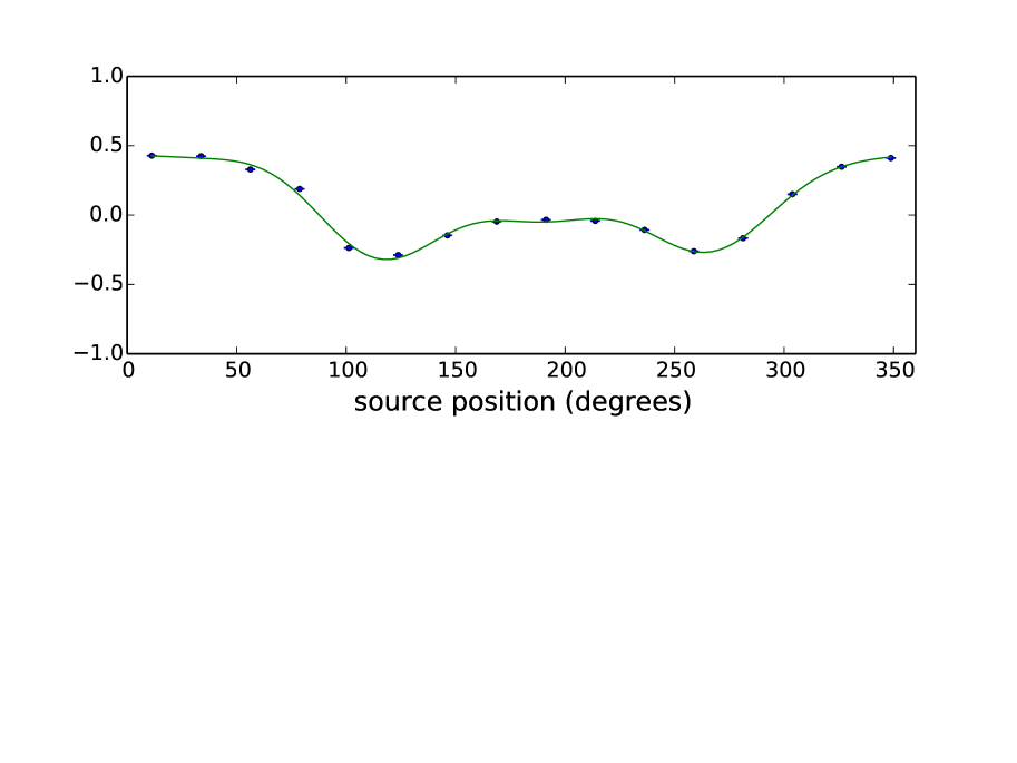
Figure 3: Detector response for a single module for 16 azimuthally equidistant source positions. To emphasize the modulation, count rates have been divided by the average value and 1.0 has been subtracted. The fit is an eleven-component Fourier series.

The response curves for all eight modules are shown in Figure 4. The curves are very similar, differing primarily by a phase which is the result of the relative orientation of the module.

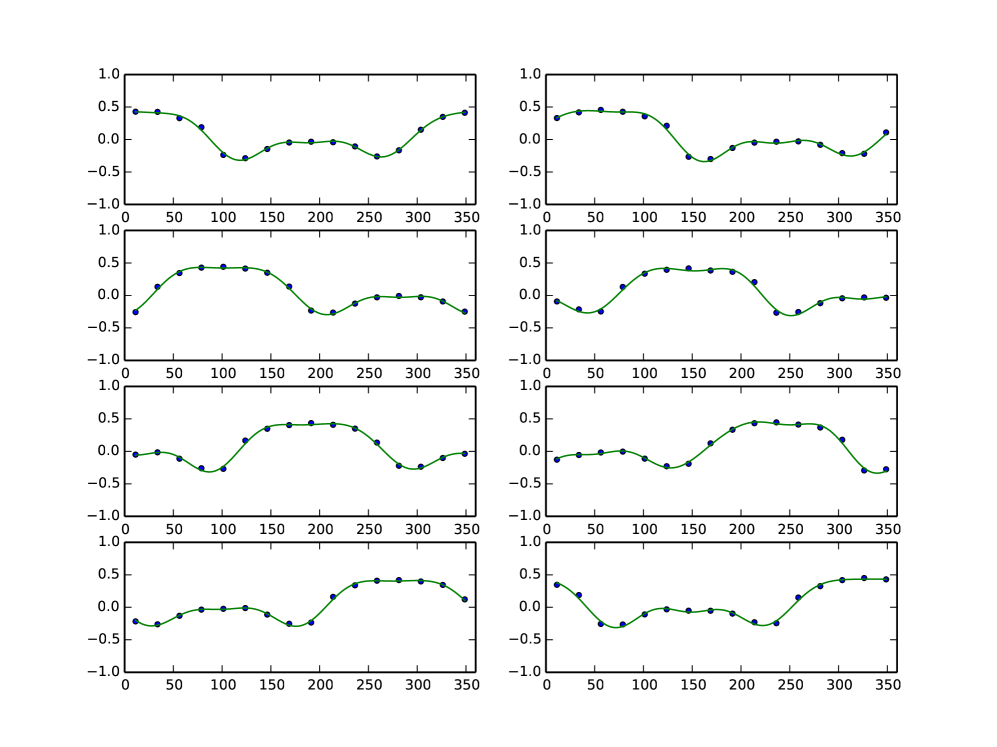
Figure 4: As in Figure 3 but for all eight modules.

We can quantify this by shifting the 16 calibration points for each module by the appropriate multiple of 45 degrees, computing the average value of the eight points at each angle, and plotting the residuals from these averages, as in Figure 5. The resulting distribution is well fit by a Gaussian with $\sigma=0.017\pm 0.002$, which is consistent with the average value of the uncertainities on the calibration points.

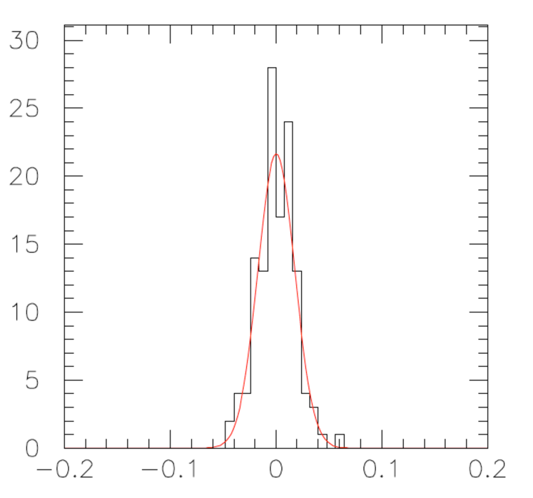
Figure 5: A histogram of the deviations of angle-shifted calibration points from their averages, as described in the text, demonstrating the similarity of the calibration curves shown in Figure 4. The horizontal scale is the same as the vertical scales in Figures 3 and  4. The fitted Gaussian has $\sigma=0.017\pm 0.002$.

3.2 Single-Source Detection

Having used the first 50 sets of count-rates vs. source position to produce the calibration curves shown in Figure 4, we used the remaining 250 sets, in various combinations, to study single-source detection.

To determine the angle of a source from the rates one minimizes the $\chi^{2}$, which is given by

$\chi^{2}=\Sigma(r_{i}-f_{i}(\phi))^{2}/\sigma_{i}^{2}$.

Where $r_{i}$ is the rate in counter $i$, $f_{i}(\phi)$ is the value of the Fourier series for counter $i$ at angle $\varphi$ and $\sigma_{i}$ is the uncertainty on $r_{i}$, derived assuming Poisson statistics from the scaler value. The minimization is done numerically by stepping through a set of 180 $\varphi$ values spaced by 2 degrees.

The technique is illustrated in Figure 6 where the $\chi^{2}$ per degree-of-freedom value is plotted vs. angle for the 180 trials. For this curve, 10 two-second data sets were combined to simulate a 20-second integration time. A single minimum is clearly visible. This highlights the utility of this method. The simple shape of the curve provides powerful visual feedback to the user since multiple dips or a single but broader dip would indicate that there are multiple sources, an extended source, or levels of background comparable to the source intensity. The time spent in calculating the 180 trials, using look-up tables for much of the work, is negligable in comparison to the data acquisition time.

The step value corresponding to the smallest $\chi^{2}$ value is used as the estimator of the angle. To obtain an estimate of the resolution of this procedure, the process is repeated 24 times using the rest of the data. A histogram of the extracted $\varphi$ values, for a single source position, is shown in Figure 7. We use the means and RMS values from a series of 16 such distributions, each made with the source at a different angle, to investigate linearity and resolution.

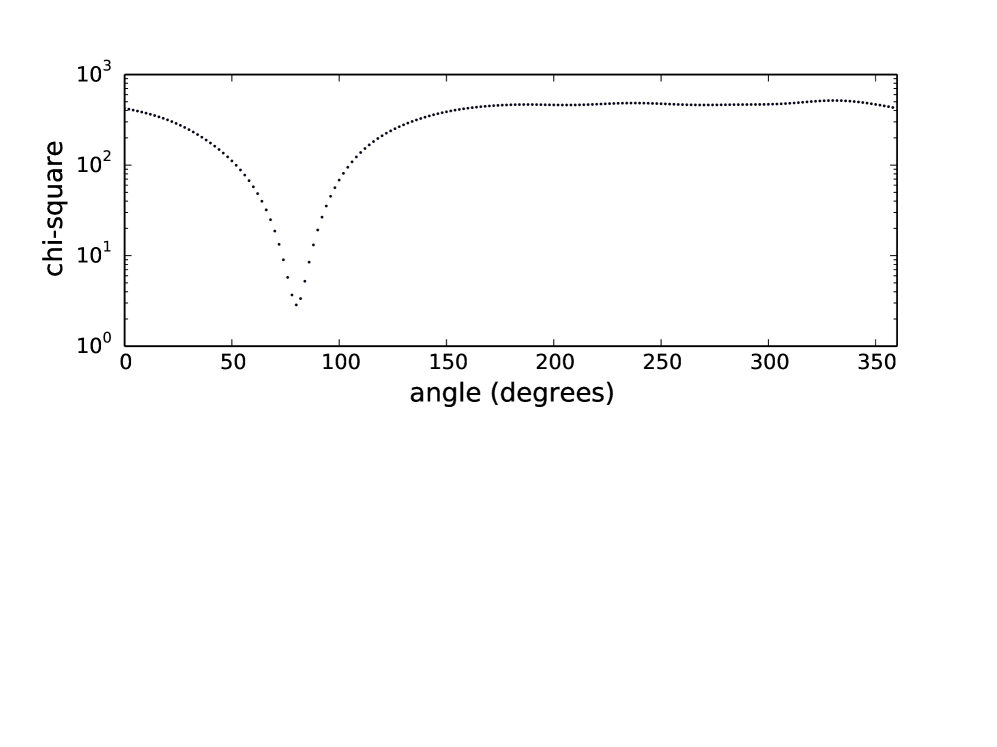
Figure 6: $\chi^{2}$/DOF values as a function of angle. The minimum occurs at the angle corresponding to the direction of the source.

Figure 7: Distribution of phi values for 25 20-second integrations made at at the same angle.

A linear function of the angle to the source can be fit to the means of distributions like the one shown in Figure 7. Figure 8 shows the residuals from such a fit vs. the source position. There is no evidence for non-linearity.

Figure 8: Residuals from a linear fit of estimated angle vs. known source position. The horizontal line is to guide the eye.

Figure 9 shows the RMS values from histograms like the one in Figure 7 vs. the source position, indicating that there is no systematic trend to the angular resolution as a function of source angle. The mean value is 1.05 $\pm$ 0.02 degrees for our 20-second integration time.

To study the effect of integration time on the angular resolution we used a large set of simulated data made by generating random numbers having the same means and widths as the count rates in our data set. We used these, along with the same calibration parameters that were used for obtaining the results in Figures 8 and 9, to perform the same analysis on data sets with different integration times. The results are displayed in Figure 10. The angular resolution improves with statistics but at a rate less than the square-root of the integration time - the power law fit gives an index of -0.39 $\pm$ 0.02.

The curve shows no sign of reaching a constant value as integration time increases. This is because we are plotting the RMS values of distributions like that in Figure 7. Once these drop below a certain level the resolution is dominated by the systematic scatter like that seen in Figure 8. As the error bars on the points in that plot decrease with increasing statistics one can see the systematics more clearly. These can arise from differences in the modules, errors in construction geometry and other sources - to attain better than degree-scale accuracy requires more attention to detail and is beyond the scope of this study.

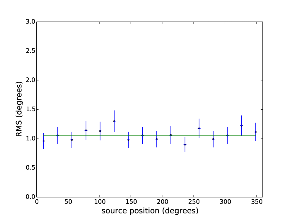
Figure 9: RMS of the estimated-angle distribution vs. source position.

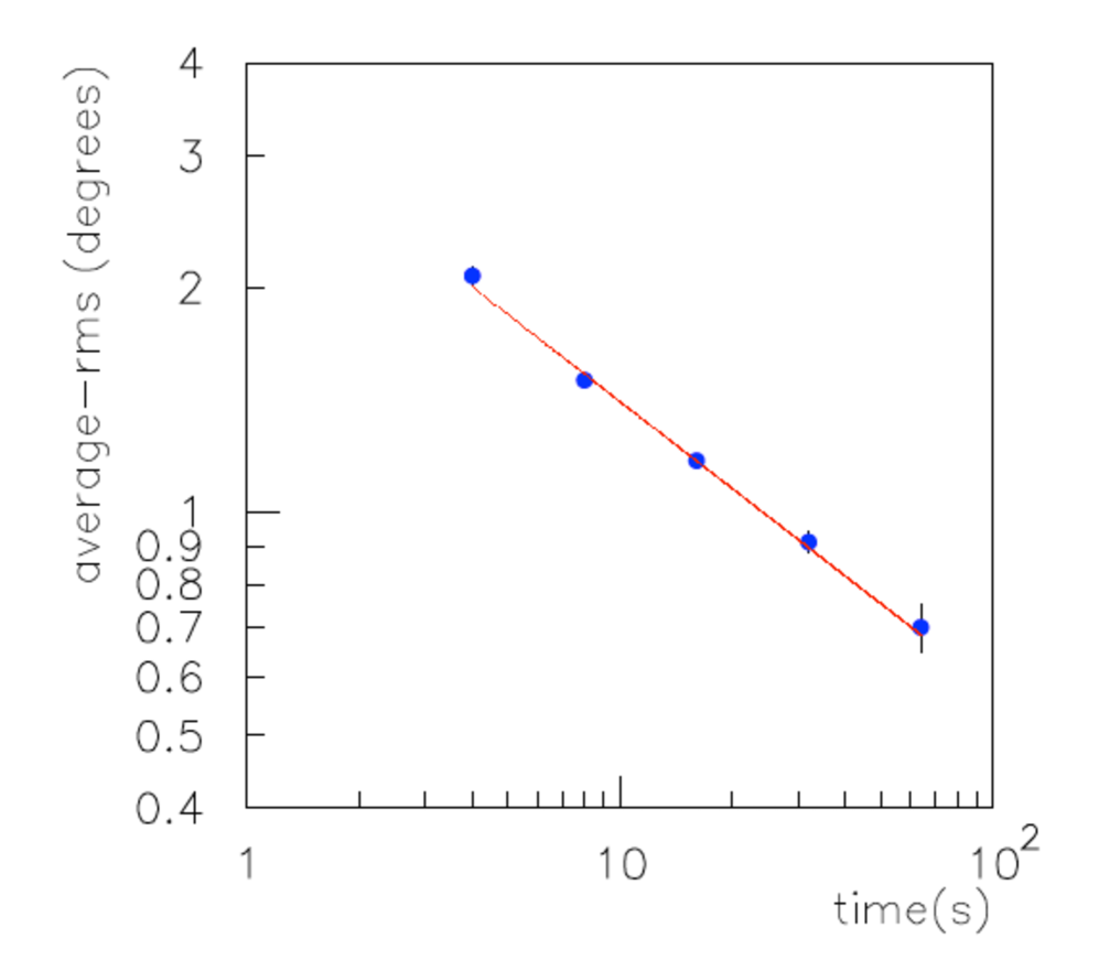
Figure 10: Average RMS of the estimated-angle distributions as a function of the integration time. The power-law fit has an index of -0.39 $\pm$ 0.02

3.3 Background Considerations

We have investigated the behaviour of the instrument in the presence of background from naturally occuring radioactive material (NORM). We used the same data as in the previous section but for each set of readings we added extra counts to the number reported by each of the eight modules. The amount was simply a Poisson-fluctuated fraction of the eight-module average. Given that this background is constant, up to statistical fluctuations, for each module it adds an overall offset but does not affect the modulation effect except to enlarge the statistical uncertainties on the count rates.

4 Multiple Sources

We investigated the effect of multiple sources at different locations with simulations and with test runs made with two sources of comparable intensity. The effect of extra sources is to distort the $\chi^{2}$ vs. angle curve, like the one shown in Figure 6, immediately alerting the user that there are complications.

This is illustrated in Figure 11 where we have combined our test files from two different angles to simulate the effects of two sources of different strengths. In the upper left panel the $\chi^{2}$ vs. angle for a single source is plotted. In subsequent panels the effects of a source 180 degrees away are included, with the relative strength of the second source increasing linearly, until the lower right panel where the two sources have the same intensity.

To extract quantitative results a more sophisticated analysis where a hyper-grid involving a number of sources with different locations and intensities is searched could be used. If the sources are isotopically different, a cut on a spectral feature such as the photopeak seen in Figure 2 could be used to reduce the search space. However, this would require more sophisticated electronics.

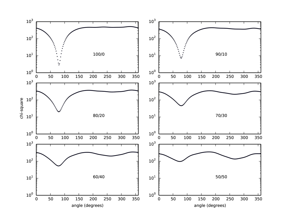
Figure 11: Simulations of the effect of an additional source located 180 degrees from the main source. In each panel, the relative intensities of the sources are given by the numbers displayed. The integration time is fixed at 20 seconds.

5 Behaviour at Greater Distances

The motivation for developing this instrument was to aid in the deployment of a Compton imager [1, 2, 3, 4]. A design specification for that imager was to locate a 10 mCi point source at a distance of 40 m to within a degree within one minute.

The studies performed here were done in a small laboratory and necessarily involved a geometry where the distance to the source was of the same order as the size of the detector. For the application envisaged the geometry will be ‘far-field’ so the calibration curves seen in Figure 4 will be slightly modified; the modulation features become sharper.

We note that given the attenuation in air of 662 keV photons, and the reduction in solid angle, a Cs-137 source would need to have an activity of approximately 37 mCi to produce the same count rates as those in our tests. This means that to determine the direction to a 10 mCi source with the resolution that we have achieved in the laboratory, we would need integration times that are longer than the 20 seconds we chose for our studies. However the main task of the instrument is to provide a rough estimate ($\pm$ 5 degrees) of the direction in which to point the imager so a 20-second integration time is expected to be sufficient. A less accurate angle, provided more quickly, is preferable.

6 Conclusions

We have developed a simple detector using eight plates of CsI(Tl) scintillator to determine the azimuthal position of a source of gamma rays. The detection algorithm relies on the relative count rates for the different plates, which have a modulation that is well described by an 11-component Fourier series. In the case of a single point source the addition of uniform background degrades the angular resolution but does not introduce systematic deviations. If more than one source is present, the relative count rates do not follow the canonical modulation, but some information on the sources and their directions may be recovered depending on their number, locations and relative intensities.

The angular resolution of the detector improves with counting statistics and therefore depends on the source strength and distance and on the level of uniform background. Our measurements indicate that for 20-second integration times, a resolution of approximately one degree can be obtained for a 10 $\mu$Ci Cs-137 source at a distance of 80 cm in an environment where the NORM background is at a level comparable to the source flux. This meets our design criteria for a device that can aid in deciding the optimal deployment direction for a Compton imager.

7 Acknowledgments

Undergraduates at McGill University have tested similar devices during the development of this instrument [10]. This work has been supported through funding from the Natural Sciences and Engineering Research Council (NSERC) the Chemical, Biological, Radiological-Nuclear and Explosives, Research and Technology Initiative (CRTI Project 07-0193RD).

References

- [1] L.E. Sinclair et al, IEEE Transactions on Nuclear Science 56(2009)
- [2] P.R.B. Saull et al, Nuclear Instruments and Methods in Physics Research Section A, 679 (2012), p. 89
- [3] A.M.L. MacLeod et al, Nuclear Instruments and Methods in Physics Research Section A, 767 (2014), p. 397
- [4] L.E. Sinclair et al, IEEE Transactions on Nuclear Science, 61 (2014), p. 2745
- [5] Pendleton, G. N., et al. 1996, ApJ, 464, 606
- [6] Y. Shirakawa Nuclear Instruments and Methods in Physics Research Section B, 263 (2007), p. 58
-
[7]
Proteus, Inc. Chagrin Falls, Ohio, 44022, USA
www.proteus-pp.com -
[8]
Sens-Tech Ltd, Langley, Berkshire, SL3 8DS, UK
www.sens-tech.com - [9] S. Griffin, D. Hanna and A. Gilbert, Proc. 32nd Int. Cosmic Ray Conference (Beijing) 9, 38 (2011).
- [10] F. Cormier et al., McGill Undergrad. Science Res. J., 9, 17 (2014)