Mesochronic classification of trajectories in incompressible 3D vector fields over finite times

Abstract.

The mesochronic velocity is the average of the velocity field along trajectories generated by the same velocity field over a time interval of finite duration. In this paper we classify initial conditions of trajectories evolving in incompressible vector fields according to the character of motion of material around the trajectory. In particular, we provide calculations that can be used to determine the number of expanding directions and the presence of rotation from the characteristic polynomial of the Jacobian matrix of mesochronic velocity. In doing so, we show that (a) the mesochronic velocity can be used to characterize dynamical deformation of three-dimensional volumes, (b) the resulting mesochronic analysis is a finite-time extension of the Okubo–Weiss–Chong analysis of incompressible velocity fields, (c) the two-dimensional mesochronic analysis from Mezić et al. “A New Mixing Diagnostic and Gulf Oil Spill Movement”, Science 330, (2010), 486-–489, extends to three-dimensional state spaces. Theoretical considerations are further supported by numerical computations performed for a dynamical system arising in fluid mechanics, the unsteady Arnold–Beltrami–Childress (ABC) flow.

Marko Budišić^∗

Department of Mathematics

University of Wisconsin, Madison

Madison, WI, USA

Stefan Siegmund

Center for Dynamics & Institute of Analysis

Department of Mathematics, TU Dresden

Dresden, Germany

Doan Thai Son

Department of Probability and Statistics

Institute of Mathematics, Vietnam Academy of Science and Technology

Hanoi, Vietnam

Igor Mezić

Department of Mechanical Engineering

University of California, Santa Barbara

Santa Barbara, CA, USA

1. Introduction

Chaotic advection is the theory of material transport in fluids based in dynamical systems theory. [3, 52, 65] It is largely rooted in analysis of geometric structures in flows with a simple time-dependence, time-autonomous or periodic. Since the realization that even flows with a complicated time dependence, e.g., turbulent flows, possess organized Lagrangian structures, it has become increasingly important to detect geometric structures analogous to invariant manifolds in steady flows. In particular, detection of structures using only finite-time information about the flow has been seen as the most practically-useful direction. [32, 56, 28, 60, 21, 2, 59]

The need for analysis of geometric structures that organize advection is not purely academic. Transport of material by fluid flows played a crucial role in the fallout from several recent catastrophic events, namely, the volcanic eruption of Eyjafjallajökull (2010), the Deepwater Horizon oil spill (2010), and the nuclear disaster in Fukushima (2011). These events highlighted how important it is to detect organizing geometric structures in (near) real time from data, either measured or generated by detailed simulation models; consequently, such problems have become a very active intersection of dynamical systems and fluid dynamics.

The problem of identifying geometric structures in flows has resulted in several approaches, each focusing on a somewhat-different structure as the objective of its analysis.

The theory of Lagrangian Coherent Structures [33] (LCS) identifies barriers that organize the transport in flows with complex time-dependence. Initially, LCS were closely associated with computation of Finite-Time Lyapunov Exponent fields [60]; more recently, they have been re-formulated using a variational principle [29, 31, 5], which defines them as certain geodesic lines of the local deformation field induced by the fluid flow. This new definition allows a finer classification of LCS, both in two and three dimensions, based on the type of deformation, e.g., hyperbolic, elliptic, corresponding to different behaviors of fluid parcels in the flow. The recent review by Haller [30] gives a detailed coverage of the current state-of-the-art of techniques centered around LCS.

LCS and associated theories mostly focused on magnitude of non-rotational deformation in the flow. The rotation deformation has been classically studied by Poincaré in topological dynamics and Ruelle [58] in ergodic theory; recently, a Finite-Time Rotation Number [61] has been proposed as a useful quantity in analysis of flows. At the closing of this manuscript we were also notified of the recent work by Farazmand and Haller [16], working along the same lines.

In the effort to study the “stretch-and-fold” mechanism for chaos in finite time, most studies focus on the first-order “stretch”. Folding in finite time has not received direct attention; an exception is the study of the Finite-Time Curvature Fields [37, 38, 39]. At this point, structures observed through all these methods have been connected mostly on phenomenological basis, through comparison of visualizations, showing considerable overlap between observed structures but, also, non-negligible differences.

Magnitudes of the local material deformation are typically estimated by processing velocity gradients; they cannot be precisely computed in the absence of the detailed data about the velocity field, e.g., when the system is sampled by sparse trajectories only. In sparsely-sampled planar systems, trajectories can be represented by space-time braids — extremely-reduced, symbolic representations of trajectories. The resulting approach, known as braid dynamics [6, 2, 62] has been successful in providing lower bounds on the amount of topological deformation present in the flow, in limited-data settings. The obtained bounds have been used both in design and analysis of the material advection; unfortunately, there are currently no extensions of braid dynamics to three-dimensional flows.

Instead of looking for barriers to transport, as is the case with the LCS theory, the theory of almost-invariant sets identifies a collection of sets, fixed in space, such that the material placed in them does not leak out. These sets act as routes for the material transport. The approach is based on the Perron–Frobenius transfer operator, which models how the flow moves distributions of points, instead of individual trajectories. The Perron–Frobenius operator is always infinite-dimensional and linear; the identification of almost-invariant sets is then intimately connected with approximating its eigenfunctions. While the Perron–Frobenius operator has been a staple of the ergodic and probability theory since the early 20th century, it was introduced to the applied, non-probabilistic context by Dellnitz and Junge [11, 12] as the basis for identification of invariant sets in time-invariant dynamical systems. Since then, the theory has been expanded to include detection of almost-invariant sets of autonomous systems [18, 20], and flows with more general time dependencies [21, 19].

Spatial invariants of dynamical systems relate to infinite-time averages of functions along Lagrangian trajectories. This connection between the ergodic theory and applied mathematics was initially developed in Ref. [43]. Based on these ideas, Ref. [56] proposed that even finite-time averages of functions can enable detection of geometric structures important for fluid transport, which broadly constitutes the mesochronic, i.e., time-averaged, theory of transport in fluids. The utility of time-averages has been corroborated on numerical and experimentally-realizable flows with simple time dependence [48, 41, 47, 42, 40].

The mesochronic techniques have developed in two directions. One focuses on computations of ergodic invariant sets using long-time averages of a large set of averaged functions. [43, 48, 36, 8] The other, which we follow here, does not aim to compute all invariant sets; rather it uses much shorter averages of the velocity field itself to identify the character of the deformation, i.e., presence or absence of rotation. [46] This is in contrast with mentioned LCS and rotational theories, which describe deformation starting from analysis of the magnitude of the deformation.

Before we dive into calculations, we give a short explanation of the approach. Introductory courses in dynamical systems often discuss the stability of a stagnation point $p$ in a planar system $\dot{x}=f(x)$ by looking at its linearization $\dot{\xi}=\nabla f|_{p}\cdot\xi$ around a fixed point $p$ whose stability depends on positions of two eigenvalues of the Jacobian $\nabla f|_{p}$. Instead of computing the eigenvalues, their locations can be inferred from the trace and the determinant of $\nabla f|_{p}$. If the flow is incompressible, the trace is zero, so the determinant alone is needed for the full stability analysis. For unsteady systems this analysis may not always hold; however, Ref. [46] showed that even then similar results can be obtained by looking at the Jacobian matrix of the velocity averaged over a Lagrangian trajectory, termed the mesochronic Jacobian matrix. Away from fixed points, the calculation does not compute stability, but rather the spectral class of the Jacobian: hyperbolic (strain) or elliptic (rotation), termed mesochronic classes. Applied to prediction of the oil slick transport in the aftermath of the Deep Water Horizon spill [46], mesochronic analysis showed that regions of mesohyperbolicity correspond to jets which dispersed the slick, while mesoelliptic zones correspond to centers of eddies in which the slick accumulated. The main contribution of this paper is the extension of the mesochronic analysis to three-dimensional flows.

There are several connections of the mesochronic analysis with other approaches.

• On a fundamental level, averages of functions along trajectories are intimately related to spectral properties of the Koopman operator [35, 45, 44], which is adjoint to the mentioned Perron–Frobenius operator.

• Greene [27, 26] defined the residue criterion in order to predict the order of destruction of Kolmogorov–Arnold–Moser (KAM) tori in perturbed Hamiltonian maps. The computation of the residue is almost identical to that of the mesohyperbolicity indicator for 2D flows. The three-dimensional version of the residue criterion [17] also resembles mesochronic indicators introduced here.

• An analysis of oceanic flows based on the Jacobian of the instantaneous, i.e., non-averaged, velocity is well-known as Okubo–Weiss–Chong partition [51, 64, 9]; this is the limit of the mesochronic theory as the averaging time $T\to 0$.

• In the other extreme, as $T\to\infty$, real parts of eigenvalues of the mesochronic Jacobian relate to Lyapunov exponents and rotation numbers). It can be shown under generic conditions, using the polar decomposition of $\nabla\psi_{T}$ that the limit of the eigenvalues of the gradient of the flow map are the Lyapunov exponents (see the heuristic discussion in [23], that can be turned into rigorous proofs using ergodic-theoretic techniques in [58], see also [1, Chapt. 3, §9])

• Finally, a recent inquiry [15] into connections with Lagrangian Coherent Structures, in a form related to an earlier work in Ref. [56], showed that the LCS techniques are capable of uncovering some of the boundaries between mesochronic classes.

The paper is organized as follows. In Section 2 we introduce the precise definitions for dynamical systems we are considering, review the basics of differential geometry needed, and re-state the Okubo–Weiss–Chong analysis in these terms. Section 3 contains the main result, the 3D mesochronic classification, while Section 4 makes connections to Lyapunov, Okubo–Weiss–Chong, and 2D mesochronic analyses. In Section 5 we illustrate the technique by a set of analytic and numerical examples; in particular the steady and unsteady Arnold–Beltrami–Childress flow [13]. Numerical details are given in the Appendices. The paper closes with the discussion in Section 6.

2. Preliminaries

Consider a time-varying differential equation

(1) $$\dot{x}=f(t,x)$$

with a $C^{3}$ velocity field $f:D\subset\mathbb{R}\times\mathbb{R}^{3}\rightarrow\mathbb{R}^{3}$. For an initial condition $(t_{0},x_{0})\in D$ let $t\mapsto\varphi(t,t_{0},x_{0})$ denote the solution (or trajectory) of the initial value problem (1), with $x(t_{0})=x_{0}$. Throughout the paper we assume for an arbitrary but fixed initial time $t_{0}\in\mathbb{R}$, duration $T>0$ and open set of initial values $X(t_{0})\subset\mathbb{R}^{3}$ that $\forall x_{0}\in X(t_{0})$, $t\mapsto\varphi(t,t_{0},x_{0})$ exists on the whole interval $I:=[t_{0},t_{0}+T]$.

For $t\in I$ define $X(t):=\{\varphi(t,t_{0},x_{0})\in\mathbb{R}^{3}:x_{0}\in X(t_{0})\}$ and $X:=\{(t,x)\in\mathbb{R}\times\mathbb{R}^{3}:t\in I,x\in X(t)\}$. Then $X\subset D$ by assumption und for $t_{1}\in I$ the map $\varphi(t_{0}+T,t_{0},\cdot):X(t_{0})\rightarrow X(t_{1})$ is well-defined. In particular, we define the time-$T$ map

(2) $$\psi_{T} :X(t_{0})\rightarrow X(t_{0}+T),$$

$$\psi_{T}(x) :=\varphi(t_{0}+T,t_{0},x),$$

usually called Poincaré map if the equation is periodic, i.e., if for the chosen $T$, $f(t,x)\equiv f(t+T,x)$.

We are mainly interested in finite-time dynamics for a fixed duration $T>0$ but will also investigate the instantaneous (in the zero-time limit $T\to 0^{+}$) and asymptotic (in the infinite-time limit $T\to+\infty$) dynamics, assuming the solution $\varphi(\cdot,t_{0},x_{0})$ exists on $[t_{0},\infty)$.

Observables of (1) are continuous functions $F:X\to\mathbb{R}^{n}$, which are evaluated along arbitrary solutions $t\mapsto x(t)$ on $I$. They are used to model physical measurements of a state of the system, e.g., the time trace $t\mapsto F\left(t,x(t)\right)$ might represent the ocean temperature recorded by a sensor as it is passively carried by ocean currents along the trajectory $x(t)$. A time average or trajectory average $\tilde{F}_{T}:X(t_{0})\rightarrow\mathbb{R}$ of an observable $F$ on $I=[t_{0},t_{0}+T]$, defined by

$$\tilde{F}_{T}(x_{0}):=\frac{1}{T}\int_{t_{0}}^{t_{0}+T}F(\tau,x(\tau))d\tau,$$

is a function that depends on the initial value $x(t_{0})=x_{0}$ of the trajectory $x(t)$ at time $t_{0}$. Trajectory averages depend on the duration $T>0$ and can be analyzed from the instantaneous, asymptotic, or finite-time perspective. The instantaneous case is the most obvious, as $\lim_{T\to 0}\tilde{F}_{T}(x_{0})=F(t_{0},x_{0})$, e.g., if $F$ is a component of the velocity field itself. Certain choices of $F$ can still provide valuable information, as we explain in the next paragraph. Asymptotic analysis studies ergodic averages, i.e., limits $\tilde{F}_{\infty}(x_{0}):=\lim_{T\to\infty}\tilde{F}_{T}(x_{0})$, in case they exist. Ergodic theory analyzes limits $\tilde{F}_{\infty}$ of observables $F$ which are specified only in general terms, e.g., only by the space of functions from which they are drawn. Even in such general cases valuable information can be recovered, e.g., on time-invariant measures on the state space. [48, 8]

On the other hand, choosing a particular observable can provide us with more detailed information. Since the components of the velocity field $f(t,x)=[f_{1}(t,x),\allowbreak f_{2}(t,x),\allowbreak f_{3}(t,x)]^{\top}$ are themselves continuous functions on the time-state space $X\subset\mathbb{R}\times\mathbb{R}^{3}$, they are observables. One could argue that they are the most distinguished observables for analysis of dynamical systems, as they directly provide dynamical information about the behavior of the system. We adopt the velocity-as-observable viewpoint and analyze the time average of the velocity field, which was termed mesochronic velocity [46]. We note that the values of the mesochronic velocity appear as quantities of interest in [56] while [46] is the first to look into their gradients.

Definition 2.1 (Mesochronic velocity and mesochronic Jacobian).

The mesochronic velocity $\tilde{f}:X(t_{0})\subset\mathbb{R}^{3}\rightarrow\mathbb{R}^{3}$ of (1) on $I=[t_{0},t_{0}+T]$ is given by

(3) $$\tilde{f}_{T}(x):=\frac{1}{T}\int_{t_{0}}^{t_{0}+T}f\left(\tau,\varphi(\tau,t_{0},x)\right)d\tau.$$

The Jacobian matrix $\nabla\tilde{f}_{T}$ containing partial spatial derivatives ${[\nabla\tilde{f}_{T}]}_{ij}\allowbreak:=\partial{[\tilde{f}_{T}]}_{i}/\partial x_{j}$ is termed the mesochronic Jacobian.

Note that the spatial derivatives and the averaging over trajectories do not commute, i.e., $\nabla\tilde{f}_{T}$ is not equal to the average of the instantaneous Jacobian over trajectories.

The mesochronic velocity in the instantaneous limit $\tilde{f}_{T}\xrightarrow{T\to 0^{+}}f$ coincides with the velocity field $f$. The asymptotic limit for $T\to\infty$ exists in many cases, for example, if the dynamical system is autonomous and volume-preserving on a compact domain.

We use the mesochronic velocity to determine the character of the evolution of a material volume (see Section 2.1) by an incompressible dynamical system, which satisfies the Liouville condition

(4) $$(\nabla\cdot f)(t,x)=\operatorname{tr}\nabla f(t,x)\equiv 0.$$

Although the limits $T\to 0^{+}$ and $T\to\infty$ have been studied classically, neither theory is applicable to transient behavior. On the other hand, the finite-time analysis of the mesochronic velocity recovers the character of the time-$T$ map $\psi:X(t_{0})\rightarrow X(t_{0}+T)$, which captures transients at the time-scale $T$ [46].

2.1. Deformation of a volume cell under a diffeomorphism

We now briefly review basic differential geometry that characterizes deformation under a volume-preserving diffeomorphism $\psi$ using the spectral class of its Jacobian $\nabla\psi$. This theory is later applied to time-$T$ maps $\psi_{T}$ of dynamical systems over finite time intervals.

Let $\psi:U\to V$ be a diffeomorphism between two open subsets $U\subset\mathbb{R}^{3}$, $V\subset\mathbb{R}^{3}$, with the usual volume measure on $\mathbb{R}^{3}$. We are interested in deformation of an infinitesimal volume cell surrounding $x\in U$ as $x\mapsto\psi(x)$. The central object of our interest is the Jacobian matrix $\nabla\psi:U\to\mathbb{R}^{3\times 3}$. It is a basic result in differential geometry that volumes of a set $S\subset U$ and its image $\psi(S)\subset V$ are equal if and only if $\left\lvert{\det\nabla\psi(x)}\right\rvert\equiv 1$. We now restrict our attention to orientation- and volume-preserving maps $\psi$, i.e., maps for which $\det\nabla\psi\equiv 1$.

At the coarsest level, we distinguish between a hyperbolic deformation, when the volume cell is deformed along all three spatial dimensions, and the opposite, non-hyperbolic character. Let $\mu_{1},\mu_{2},\mu_{3}\in\mathbb{C}$ denote the eigenvalues of $\nabla\psi$, assuming $\left\lvert{\mu_{1}}\right\rvert\leq\left\lvert{\mu_{2}}\right\rvert\leq\left\lvert{\mu_{3}}\right\rvert$. Different fields of mathematics may interpret presence or absence of hyperbolicity differently, e.g., as the material deformation in continuum mechanics, or stability of the map in dynamical systems and control. Since our analysis could include both domains, we refer to presence/absence of hyperbolicity, and their sub-classification (see below) as the spectral character of the diffeomorphism.

Definition 2.2 (Hyperbolicity).

The map $\psi$ is hyperbolic at $x$ if no eigenvalues $\mu_{1},\mu_{2},\mu_{3}$ of the Jacobian $\nabla\psi(x)$ lie on the unit circle in the complex plane, i.e., $\forall\ i=1,2,3$, $\left\lvert{\mu_{i}}\right\rvert\not=1$. Otherwise, it is non-hyperbolic at $x$. In particular, if all eigenvalues lie on the unit circle, i.e., $\forall\ i=1,2,3$, $\left\lvert{\mu_{i}}\right\rvert=1$, the non-hyperbolic map is elliptic.

Depending on the complexity of eigenvalues, we further distinguish sellar (saddle-like) and helical (spiral/helix-like) character of the deformation under $\psi$.

Definition 2.3 (Sellar and helical deformation).

The map $\psi$ is sellar at $x$ if all eigenvalues $\mu_{1},\mu_{2},\mu_{3}$ of the Jacobian $\nabla\psi(x)$ are real and non-defective (their algebraic and geometric multiplicities match). If, instead, there is a pair of complex-conjugate eigenvalues, the map is helical (spiral-like) at $x$.

Deformation at a sellar point exhibits three distinct spatial axes, meeting at $x$, whose directions are preserved under $\psi$. The directions of preserved spatial axes correspond to real-valued eigenvectors of $\nabla\psi$, while the associated (real) eigenvalues $\mu$ determine whether the points along the axes are moving away from $x$, $(\left\lvert{\mu}\right\rvert>1)$, moving towards $x$, $(\left\lvert{\mu}\right\rvert<1)$, or remain neutral $(\left\lvert{\mu}\right\rvert=1)$.

Deformation at a helical point exhibits only a single preserved spatial axis, around which a volume cell is rotated, resulting in a single real-valued eigenvalue. As $\nabla\psi(x)$ is a real matrix, any complex eigenvalues must arise in conjugate pairs, $\mu,\,\bar{\mu}$. The modulus of the complex pair again determines expansion or contraction of the material in the rotation plane, while the real and imaginary components of the associated eigenvector pair span the rotation plane.

Since we restrict our analysis to volume-preserving maps $\psi$, existence of an eigenvalue inside the unit circle (contraction) necessarily means that at least one other eigenvalue lies outside of the unit circle (expansion), as $\left\lvert{\det\nabla\psi}\right\rvert=\left\lvert{\mu_{1}\mu_{2}\mu_{3}}\right\rvert\equiv 1$. All possible combinations are enumerated in Definition 2.4 in which we use the symbols $+$ and $-$ to denote expansion and contraction directions, respectively.

Definition 2.4 (Spectral classes).

Let $\psi:U\to V$ be a volume- and orientation-preserving diffeomorphism, $x\in U$ a point, and $\nabla\psi(x)$ the Jacobian of $\psi$ at $x$ with eigenvalues $\mu_{i}$, ordered as $\left\lvert{\mu_{1}}\right\rvert\leq\left\lvert{\mu_{2}}\right\rvert\leq\left\lvert{\mu_{3}}\right\rvert$. The class of the point $x$ is determined according to Table 1 by the number of eigenvalues of $\nabla\psi(x)$ that are inside and on the unit circle.

Class	Condition
$\bm{[-++]}$ sellar (hyp. saddle)	$\mu_{1,2,3}\in\mathbb{R}$ and $\left\lvert{\mu_{1}}\right\rvert<1<\left\lvert{\mu_{2}}\right\rvert<\left\lvert{\mu_{3}}\right\rvert$,
$\bm{[--+]}$ sellar (hyp. saddle)	$\mu_{1,2,3}\in\mathbb{R}$ and $\left\lvert{\mu_{1}}\right\rvert<\left\lvert{\mu_{2}}\right\rvert<1<\left\lvert{\mu_{3}}\right\rvert$,
$\bm{[-++]}$ helical (hyp. spiral)	$\mu_{1}\in\mathbb{R},\ \mu_{2}=\bar{\mu}_{3}\not\in\mathbb{R}$ and $\left\lvert{\mu_{1}}\right\rvert<1<\left\lvert{\mu_{2}}\right\rvert=\left\lvert{\mu_{3}}\right\rvert$,
$\bm{[--+]}$ helical (hyp. spiral)	$\mu_{1}=\bar{\mu}_{2}\not\in\mathbb{R},\ \mu_{3}\in\mathbb{R}$ and $\left\lvert{\mu_{1}}\right\rvert=\left\lvert{\mu_{2}}\right\rvert<1<\left\lvert{\mu_{3}}\right\rvert$,
Neutral saddle	$\mu_{1,2,3}\in\mathbb{R}$ and $\left\lvert{\mu_{1}}\right\rvert<1=\left\lvert{\mu_{2}}\right\rvert<\left\lvert{\mu_{3}}\right\rvert$,
Neutral helix	$\mu_{1}=\bar{\mu}_{2}\not\in\mathbb{R},\ \mu_{3}\in\mathbb{R}$ and $\left\lvert{\mu_{i}}\right\rvert\equiv 1$,
Pure shear	$\mu_{1}=\mu_{2}=\pm 1$, $\mu_{3}=1$ and $\nabla\psi$ is defective,
Pure reflection	$\mu_{1,2,3}\in\{-1,1\}$ and $\nabla\psi$ is not defective.

Table 1. Classification of a 3D volume-preserving diffeomorphism, depending on locations of eigenvalues $\mu_{1,2,3}$ of the Jacobian matrix (see Definition 2.4). A matrix is defective, or non-diagonalizable, when it has less than 3 linearly independent eigenvectors.

The first four classes are hyperbolic, whereas the remaining cases are non-hyperbolic. Informally, we will refer to signatures $\bm{[-++]}$ and $\bm{[--+]}$ of hyperbolic points as, respectively, flattening and elongating, due to the shape of a volume cell after application of $\psi$, as sketched in Figure 1.

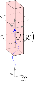
(a) $\bm{[--+]}$ sellar deformation (elongating saddle)

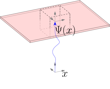
(b) $\bm{[-++]}$ sellar deformation (flattening saddle)

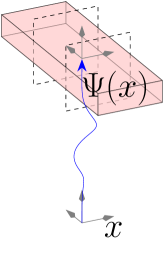
(c) Neutral sellar (neutral saddle)

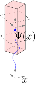
(d) $\bm{[--+]}$ helical deformation (elongating spiral)

(e) $\bm{[-++]}$ helical deformation (flattening spiral)

(f) Neutral helical (neutral spiral)

Figure 1. Sketches of deformation depending on the spectral class of a volume-preserving diffeomorphism $\psi$ at the point $x\in U$ (see Definition 2.4). Note that the initial and final axes do not need to be parallel in general. Pure shear and reflection (including the identity) are not sketched.

2.2. Instantaneous deformation by a dynamical system

We now apply the classification outlined in Section 2.1 to the time-$T$ map $\psi_{T}$ defined in (2) for a fixed time interval $T$ to recover the Okubo–Weiss–Chong [51, 64, 9] criterion for classification of velocity fields. Instead of forming the classification of $\psi_{T}$ based on properties of $\nabla\psi_{T}$, we chose instead to base our approach on properties of the mesochronic Jacobian $\nabla\tilde{f}_{T}$, resulting in criteria whose expressions are consistent across all time scales $T$.

Instantaneous classification refers to the infinitesimally small time interval length $T$ for which the class of $x\in\mathbb{R}^{3}$ under $\psi_{T}$ can be inferred from the spectrum of the Jacobian $\nabla f(t_{0},x)$, through the connections with $\nabla\psi_{T}$. Both Jacobians are $3\times 3$ matrices; for a general such matrix $M$, the characteristic polynomial is given by

(5) $$P_{M}(s) =\det\left(s\mathrm{Id}-M\right)=s^{3}-s^{2}\operatorname{tr}M+s\operatorname{tr}\operatorname{Cof}M+\det M$$

where

(6) $$\operatorname{tr}M =\sum_{i}s_{i},\qquad\det M=\prod_{i}s_{i},$$

(7) $$\operatorname{tr}\operatorname{Cof}M =\sum_{i}\frac{\det M}{s_{i}}=\frac{1}{2}(\operatorname{tr}M^{2}-(\operatorname{tr}M)^{2})$$

The coefficient $\operatorname{tr}\operatorname{Cof}M$ is the cofactor trace, also called “second trace”, in [17]; intuitively, it is the “variance” of the vector containing eigenvalues. Additionally, it follows from (7) that when $\det M=1$, the second trace is equal to the trace of matrix inverse $\operatorname{tr}\operatorname{Cof}M=\sum s_{i}^{-1}=\operatorname{tr}M^{-1}$. Further spectral properties of such matrices are summarized in the Appendix A.

As mentioned in Definition 2.4, spectral class of the time-$T$ map is determined by locations of eigenvalues of $\nabla\psi_{T}$ which, in turn, are roots of the characteristic polynomial $P_{\psi}(\mu)=\det\left(\mu\mathrm{Id}-\nabla\psi_{T}(x)\right)$.

Expanding $\nabla\psi(x)$ into a Taylor series around $T=0$ yields

(8) $$\nabla\psi_{T}(x) =\mathrm{Id}+T\nabla f(t_{0},x)+\mathcal{O}(T^{2})$$

$$\approx\mathrm{Id}+T\nabla f(t_{0},x),$$

for $T\approx 0$. Consequently

$$P_{\psi}(\mu) =\det\left[(\mu-1)\mathrm{Id}-T\nabla f(t_{0},x)\right]$$

$$=T^{3}P_{f}\left(\frac{\mu-1}{T}\right),$$

for $T\approx 0$, where $P_{f}(\lambda)=\det\left(\lambda\mathrm{Id}-\nabla f(t_{0},x)\right)=\lambda^{3}-t_{f}\lambda^{2}+m_{f}\lambda-d_{f}$ is the characteristic polynomial of the Jacobian matrix $\nabla f$ of the instantaneous velocity field. In all cases, Jacobian matrices are evaluated at the time-space point $(t_{0},x)$ which is suppressed in notation.

Incompressibility of the flow implies

(9) $$t_{f}\equiv 0\text{\quad and \quad}d_{\Psi}\equiv 1,$$

and therefore the spectral character depends only on the determinant $d_{f}$ and the sum of minors $m_{f}$ of the velocity field Jacobian $\nabla f$. We now state the Okubo–Weiss–Chong criteria, using terminology specified in Definition 2.4.

Theorem 2.5 (Okubo–Weiss–Chong [9]).

From the Jacobian of the velocity field (velocity gradient tensor) $\nabla f(t_{0},x)$, compute its determinant $d_{f}=\det\nabla f(t_{0},x)$, and cofactor trace $m_{f}=\operatorname{tr}\operatorname{Cof}\nabla f(t_{0},x)$. For $T\to 0$, the point $(t_{0},x)\in I\times\mathbb{R}^{3}$ is hyperbolic if and only if

$$d_{f}\not=0.$$

Hyperbolic points can be further classified into four subclasses, depending on signs of the determinant $d_{f}$ and the quantity $27d_{f}^{2}+4m_{f}^{3}$, as listed in Table 2.

$d_{f}$	$27d_{f}^{2}+4m_{f}^{3}$	OWC class
$-$	$-$	$\bm{[-++]}$ saddle
$-$	$+$	$\bm{[-++]}$ helix
$+$	$-$	$\bm{[--+]}$ saddle
$+$	$+$	$\bm{[--+]}$ helix

Table 2. Okubo–Weiss–Chong classification based on signs of quantities in the first two columns (see Theorem 2.5).

The analogous result for planar dynamics is known as the Okubo–Weiss criterion [51, 64].

3. Mesochronic classification

The Okubo–Weiss–Chong criterion (Theorem 2.5) classifies the points in the domain of the time-$T$ map $\psi_{T}$ according to the spectral character of the Jacobian $\nabla f$ of the velocity field. In general, the spectral character of $\nabla\psi_{T}$ for $T$ away from $0$ will not be approximated well by the spectral character of $\nabla f$, except in extremely slowly varying flows. In order to capture both deformation at small and large $T$, we replace $\nabla f$ by the Jacobian $\nabla\tilde{f}_{T}$ of the mesochronic velocity $\tilde{f}_{T}$, defined as the Lagrangian average of the velocity $f$ over the duration $T$:

(10) $$\tilde{f}_{T}(x):=\frac{1}{T}\int_{t_{0}}^{t_{0}+T}f\big{(}\tau,\varphi(\tau,t_{0},x)\big{)}d\tau.$$

To see why $\nabla\tilde{f}_{T}(x)$ plays an important role in our analysis, we write the solution $\varphi(t,t_{0},x)$ in its integral form

(11) $$\varphi(t,t_{0},x)=x+\int_{t_{0}}^{t}f\big{(}\tau,\varphi(\tau,t_{0},x)\big{)}d\tau,$$

which is a consequence of the fundamental theorem of calculus. The same integral appears both in (10) and (11), which we use to write the time-$T$ map as

(12) $$\psi_{T}(x)=\varphi(t_{0}+T,t_{0},x)=x+T\tilde{f}_{T}(x),$$

and hence

(13) $$\nabla\psi_{T}(x)=\mathrm{Id}+T\nabla\tilde{f}_{T}(x).$$

Comparing with (8), $\nabla\psi_{T}(x)\approx\mathrm{Id}+T\nabla f(t_{0},x)$ which is valid for $T\approx 0$, we see that for general time intervals $[t_{0},t_{0}+T]$ the mesochronic velocity Jacobian $\nabla\tilde{f}_{T}(x)$ plays the same role as the velocity field Jacobian $\nabla f(t_{0},x)$ did for intervals of infinitesimal length.

In analogy to Okubo–Weiss–Chong, we classify $x\in X(t_{0})\subset\mathbb{R}^{3}$ under the action $\psi_{T}$ using only information obtained from the mesochronic velocity and its Jacobian $\nabla\tilde{f}_{T}(x)$.

Definition 3.1 (Mesochronic classes).

Given a fixed time interval $[t_{0},t_{0}+T]$, the point $x\in X(t_{0})\subset\mathbb{R}^{3}$ is mesohyperbolic if it is hyperbolic with respect to the diffeomorphism $\psi_{T}$ (time-$T$ map), i.e., no eigenvalues of $\nabla\psi_{T}(x)$ lie on the unit circle in the complex plane. Otherwise, $x$ is non-mesohyperbolic.

Similarly, the mesochronic class of $x$ is the spectral class of $\psi_{T}$ at $x$, as specified by Definition 2.4.

As explained in Section 2.1, the Liouville incompressibility results in only two, instead of three, “axes” in which we understand the spectral class of $\psi_{T}$:

1. number of contracting directions, indicated by labels $\bm{[-++]}$ and $\bm{[--+]}$.

2. presence of a rigid rotation, indicated by helix vs. saddle split.

The four mesohyperbolic classes are formed by choosing an option along each of the axes above, with the non-hyperbolic classes acting as boundary cases between them.

For conceptual and computational reasons we will formulate quantities $\Sigma$ and $\Delta$, each corresponding to one of the “axes” above, such that the signs of their values sort the finite-time dynamics around $x$ into mesochronic classes. The number of contracting directions will be detected by $\Sigma$, the presence of rotation by $\Delta$.

Theorem 3.2 (Mesochronic classification).

Let $\nabla\tilde{f}_{T}(x)$ be the mesochronic Jacobian matrix for the dynamics at the point $x\in X(t_{0})\subset\mathbb{R}^{3}$ and for the time interval $[t_{0},t_{0}+T]$ and $P_{\tilde{f}}(\lambda):=\lambda^{3}-t_{\tilde{f}}\lambda^{2}+m_{\tilde{f}}\lambda-d_{\tilde{f}}$, the characteristic polynomial of the matrix $\nabla\tilde{f}_{T}(x)$. Define

(14) $$\Sigma:= \ \frac{d_{\tilde{f}}T^{3}}{8-2m_{\tilde{f}}T^{2}-3d_{\tilde{f}}T^{3}}$$

$$\Delta:= -4d_{\tilde{f}}^{4}T^{12}-12d_{\tilde{f}}^{3}m_{\tilde{f}}T^{11}$$

$$-13d_{\tilde{f}}^{2}m_{\tilde{f}}^{2}T^{10}-6d_{\tilde{f}}m_{\tilde{f}}^{3}T^{9}$$

$$+(18d_{\tilde{f}}^{2}m_{\tilde{f}}-m_{\tilde{f}}^{4})T^{8}+18d_{\tilde{f}}m_{\tilde{f}}^{2}T^{7}$$

$$+(27d_{\tilde{f}}^{2}+4m_{\tilde{f}}^{3})T^{6}.$$

If $8-2m_{\tilde{f}}T^{2}-3d_{\tilde{f}}T^{3}=0$, then $x$ is non-mesohyperbolic of the neutral-saddle type.

If $\Sigma$ is finite, the point $x$ is classified into mesochronic classes according to Table 3. Mesohyperbolic classes are those for which $\Sigma$ is finite and $\Sigma\not=0$, i.e., for which both

(15) $$d_{\tilde{f}}\not=0\text{ and }8-2m_{\tilde{f}}T^{2}-3d_{\tilde{f}}T^{3}\not=0.$$

The distinction between the shear and the boundary saddle class when $\Delta=0$ depends on eigenvectors of the mesochronic Jacobian and cannot be made purely based on the spectrum.

$\Sigma$	$\Delta$	Mesochronic class
$-$	$-$	$\bm{[-++]}$ mesosellar
$-$	$0$	$\bm{[-++]}$ mesosellar or shear
$-$	$+$	$\bm{[-++]}$ mesohelical
$0$	$-$	neutral mesosellar
$0$	$0$	pure reflection
$0$	$+$	neutral mesohelical
$+$	$-$	$\bm{[--+]}$ mesosellar
$+$	$0$	$\bm{[--+]}$ shear or mesosellar
$+$	$+$	$\bm{[--+]}$ mesohelical

Table 3. Mesochronic classification based on signs of $\Sigma$ and $\Delta$ (see Theorem 3.2). The classes with $\Sigma\not=0$ are mesohyperbolic. The class for $\Sigma=\pm\infty$ is the neutral (non-mesohyperbolic) saddle.

The proof of the theorem will be the result of two lemmas:

• Lemma 3.3 defines $\Sigma$ and $\Delta$ using coefficients of the characteristic polynomial of the time-$T$ map Jacobian matrix $\nabla\psi_{T}(x)$.

• Lemma 3.4 establishes relations between characteristic coefficients of $\nabla\psi_{T}(x)$ and characteristic coefficients of $\nabla\tilde{f}_{T}(x)$.

Lemma 3.3.

Let $\psi_{T}(x)$ be the time-$T$ map at a point $x\in X(t_{0})\subset\mathbb{R}^{3}$ over the time interval $[t_{0},t_{0}+T]$ and $P_{\psi}(\mu):=\mu^{3}-t_{\psi}\mu^{2}+m_{\psi}\mu-d_{\psi}$, the characteristic polynomial of the Jacobian matrix $\nabla\psi_{T}(x)$. Define

(16) $$\Sigma= \ \frac{t_{\psi}-m_{\psi}}{t_{\psi}+m_{\psi}+2},$$

$$\Delta= \ 4(m_{\psi}^{3}+t_{\psi}^{3})-m_{\psi}^{2}t_{\psi}^{2}-18m_{\psi}t_{\psi}+27.$$

If $m_{\psi}+t_{\psi}+2=0$, then $x$ is non-mesohyperbolic of neutral-saddle type.

If $\Sigma$ is finite, then the point $x$ is classified into mesochronic classes defined by Table 3. Mesohyperbolic classes are those for which $\Sigma$ is finite and $\Sigma\not=0$, i.e.,

$$t_{\psi}-m_{\psi}\not=0\quad\text{and}\quad t_{\psi}+m_{\psi}+2\not=0.$$

Remark 1.

The trace $t_{\psi}$ and the determinant $d_{\psi}$ of the Jacobian matrix $\nabla\psi_{T}$ are commonly encountered in matrix analysis due to their simple relationships to eigenvalues. To interpret the cofactor trace $m_{\psi}$ we can expand it as:

$$m_{\psi} =\sum_{j\not=k}\mu_{j}^{\ast}\mu_{k}^{\ast}=\mu_{1}^{\ast}\mu^{\ast}_{2}\mu^{\ast}_{3}\sum_{i=1}^{3}\frac{1}{\mu_{i}^{\ast}}$$

$$=\det\nabla\psi_{T}\cdot\operatorname{tr}\left[{(\nabla\psi_{T})}^{-1}\right].$$

Under an incompressible flow ($\det\nabla\psi_{T}\equiv 1$) the cofactor trace $m_{\psi}$ is the trace of the inverse of the time-$T$ map Jacobian, as discussed after (7):

$$m_{\psi}=t_{\psi^{-1}}.$$

Additionally, we can clarify the meaning of $\Sigma$. Rewrite (16) as

$$\Sigma=1-2{\left(\frac{t_{\psi}+1}{m_{\psi}+1}+1\right)}^{-1}.$$

Then through simple algebraic manipulation it follows that

(17) $$\operatorname{sgn}\Sigma=\operatorname{sgn}\left(\frac{t_{\psi}+1}{m_{\psi}+1}-1\right)=\operatorname{sgn}(t_{\psi}-m_{\psi}).$$

Using $m_{\psi}=t_{\psi^{-1}}$ and rewriting the expressions for $t_{\psi}$ using eigenvalues $\mu_{i}$ of the flow map Jacobian, we obtain that

(18) $$\operatorname{sgn}\Sigma\equiv\operatorname{sgn}\left[(\mu_{1}-\mu_{1}^{-1})+(\mu_{2}-\mu_{2}^{-1})-(\mu_{1}\mu_{2}-\mu_{1}^{-1}\mu_{2}^{-1})\right].$$

Proof of Lemma 3.3.

The mesochronic class of $x$ is determined by eigenvalues of the Jacobian $\nabla\psi_{T}(x)$, whose characteristic polynomial is $P_{\psi}(\mu)=\mu^{3}-t_{\psi}\mu^{2}+m_{\psi}\mu-d_{\psi},$ with determinant $d_{\psi}$, trace $t_{\psi}$, and cofactor trace $m_{\psi}$ of $\nabla\psi_{T}$ (see Appendix A).

The mesochronic class is determined by relative locations of zeros $P_{\psi}(\mu^{\ast})=0$ in reference to the unit circle and to the horizontal axis. As mentioned, converting the reference unit circle to a vertical axes simplifies the criteria, as they can then be computed solely from signs of eigenvalues. To this end, we introduce the conformal map $\Gamma(s)=\frac{1+s}{1-s}$ which maps the left half-plane in $\mathbb{C}$ to the inside of the unit circle in $\mathbb{C}$, while preserving the upper half-plane. It follows that the location of zeros of the composite function $P_{\psi}\circ\Gamma$ with respect to axes is the same as the location of zeros of $P_{\psi}$ with respect to horizontal axes and the unit circle. Note that the inverse $\Gamma^{-1}(\mu)=\frac{\mu-1}{\mu+1}$ has a pole at $\mu^{\ast}=-1$, so no finite zeros in the $s$-plane will correspond to the zero of $P_{\psi}$ at $\mu^{\ast}=-1$. For this reason, we will separately treat the case when $\nabla\psi_{T}$ has an eigenvalue at $-1$.

Assuming $P_{\psi}(-1)\not=0$, the composite function is

(19) $$[P_{\psi}\circ\Gamma](s)=\frac{n_{3}s^{3}+n_{2}s^{2}+n_{1}s+n_{0}}{{(s-1)}^{3}},$$

with coefficients

$$n_{3} =-1-t_{\psi}-m_{\psi}-\phantom{3}d_{\psi}=-t_{\psi}-m_{\psi}-2$$

$$n_{2} =-3-t_{\psi}+m_{\psi}+3d_{\psi}=-t_{\psi}+m_{\psi}$$

$$n_{1} =-3+t_{\psi}+m_{\psi}-3d_{\psi}=\phantom{-}t_{\psi}+m_{\psi}-6$$

$$n_{0} =-1+t_{\psi}-m_{\psi}+\phantom{3}d_{\psi}=\phantom{-}t_{\psi}-m_{\psi},$$

where the second equalities are obtained by incompressibility $d_{\psi}=\prod_{i=1}^{3}\mu_{i}^{\ast}=1$.

A point $x$ is non-hyperbolic whenever one of the roots of the characteristic polynomial $P_{\psi}(\mu)$ of $\nabla\psi_{T}(x)$ is on the unit circle. If $P_{\psi}(-1)\not=0$, this condition implies that a purely imaginary number $ia$, $a\in\mathbb{R}$ is a zero of $P_{\psi}\circ\Gamma$. Substituting into the numerator of $P_{\psi}\circ\Gamma$, we obtain the condition $n_{1}n_{2}-n_{0}n_{3}\not=0$ for hyperbolicity. This condition translates to a condition on the spectral coefficients of $\nabla\psi_{T}$: $t_{\psi}-m_{\psi}\not=0$. The other case for non-hyperbolicity is $P_{\psi}(-1)\not=0$, which by direct substitution into $P_{\psi}$ translates to $t_{\psi}+m_{\psi}+2\not=0$.

When $P_{\psi}(-1)\not=0$, we can proceed to a finer classification of the location of the roots of $P_{\psi}$. Due to incompressibility, there either have to be two zeros of the polynomial $P_{\psi}$ inside a circle and one outside, or vice-versa. Under a conformal transformation $\Gamma$ this condition translates into two zeros of $P_{\psi}\circ\Gamma$ having matching signs, while the third is of the opposite sign. It follows that the product of zeros $s^{\ast}_{i}$ of $P_{\psi}\circ\Gamma$ is positive when two zeros are negative, corresponding to two directions of contraction under the flow map, while it is negative when there is a single contracting and two expanding directions. By using the zeros $s_{i}^{\ast}$ of $P_{\psi}\circ\Gamma$ to factorize its numerator $\sum_{i=0}^{3}n_{i}s^{i}=n_{3}\prod_{i=1}^{3}(s-s_{i}^{\ast})$ and equating the zeroth-order coefficients one obtains $-n_{3}\prod_{i=1}^{3}s_{i}^{\ast}=n_{0}$. We therefore define an indicator $\Sigma$ as

$$\Sigma:=s_{1}^{\ast}s_{2}^{\ast}s_{3}^{\ast}=-\frac{n_{0}}{n_{3}}=\frac{t_{\psi}-m_{\psi}}{t_{\psi}+m_{\psi}+2}.$$

By this argument, $\Sigma\not=0$ implies hyperbolicity: $\Sigma>0$ implies two directions of contraction, one of expansion, while $\Sigma<0$ implies one direction of contraction, two of expansion. When $\Sigma=0$ one of the roots of $P_{\psi}$ lies on the unit circle, which we term “neutral”, while the other two directions are contracting and expanding.

The presence of rotation is indicated by the complexity of zeros of $P_{\psi}\circ\Gamma$, which is determined by the discriminant of the numerator,

(20) $$\mathcal{D}_{3D{}}=-64\big{(}4(m_{\psi}^{3}-t_{\psi}^{3})-m_{\psi}^{2}t_{\psi}^{2}-18m_{\psi}t_{\psi}+27\big{)}.$$

When $\mathcal{D}_{3D{}}>0$, all zeros are real and distinct, when $\mathcal{D}_{3D{}}<0$, two zeros are complex-conjugates of each other, when $\mathcal{D}_{3D{}}=0$, one real zero is repeated, while the third is distinct. We therefore define our second indicator $\Delta$ to be

(21) $$\Delta:=-\mathcal{D}_{3D{}}/64=4(m_{\psi}^{3}+t_{\psi}^{3})-m_{\psi}^{2}t_{\psi}^{2}-18m_{\psi}t_{\psi}+27.$$

It follows that $\Delta<0$ indicates that all eigenvalues of $\nabla\psi_{T}(x)$ are real, implying that there is no rigid rotation; $\Delta>0$ indicates that two eigenvalues are complex, so rigid rotation is present. When $\Delta=0$ two eigenvalues coincide somewhere along the real line.

Finally, we have to deal with the case when $P_{\psi}(-1)=0$ which is not covered by the $s$-complex plane as defined above, as it implies that the denominator of $\Sigma$ is zero, i.e., $t_{\psi}+m_{\psi}+2=0$. If one zero is $\mu^{\ast}_{2}=-1$, then the two others have to be $\mu_{1}^{\ast}=z$, $\mu_{3}^{\ast}=-1/z$, for some $z\in\mathbb{C}$ to satisfy incompressibility. Therefore the studied point $x$ is non-hyperbolic, with signature $[-\ 0\ +]$. Notice that if $z$ has an imaginary component, its conjugate is $\bar{z}=-1/z$, which cannot be, as $z\bar{z}\geq 0$, therefore one zero at $-1$ implies that the other two zeros are necessarily real. It follows that $P_{\psi}(-1)=0$ indicates a neutral saddle case, even if $\Sigma$ cannot be evaluated. ∎

We now relate the characteristic polynomials of $\nabla\psi_{T}$ and $\nabla\tilde{f}_{T}$.

Lemma 3.4.

The characteristic polynomial of the Jacobian matrix $\nabla\psi_{T}$ and the characteristic polynomial of the mesochronic Jacobian $\nabla\tilde{f}_{T}$ are given by the expressions

(22) $$P_{\psi}(\mu) =\mu^{3}-t_{\psi}\mu^{2}+m_{\psi}\mu-d_{\psi},$$

$$P_{\tilde{f}}(\lambda) =\lambda^{3}-t_{\tilde{f}}\lambda^{2}+m_{\tilde{f}}\lambda-d_{\tilde{f}}.$$

The coefficients are linked by the expressions

(23) $$t_{\psi} =3+Tt_{\tilde{f}}$$

$$m_{\psi} =3+2Tt_{\tilde{f}}+T^{2}m_{\tilde{f}}$$

$$d_{\psi} =1+Tt_{\tilde{f}}+T^{2}m_{\tilde{f}}+T^{3}d_{\tilde{f}},$$

where $T$ is the length of the averaging period in $\tilde{f}_{T}$.

Moreover, the incompressibility condition $d_{\psi}\equiv 1$ imposes the relation

(24) $$t_{\tilde{f}}+Tm_{\tilde{f}}+T^{2}d_{\tilde{f}}\equiv 0$$

on the coefficients of $P_{\tilde{f}}$ for $T\not=0$.

Proof.

The connection between the two Jacobian matrices $\nabla\psi_{T}$ and $\nabla\tilde{f}_{T}$ is given by relation (13): $\nabla\psi_{T}=\mathrm{Id}+T\nabla\tilde{f}_{T}$. The characteristic polynomial $P_{\psi}$ of $\nabla\psi_{T}$ can be re-written using the characteristic polynomial $P_{\tilde{f}}$ of $\nabla\tilde{f}_{T}$

$$P_{\psi}(\mu) =\ \det(\mu\mathrm{Id}-\nabla\psi_{T})=\ T^{3}\det\left(\frac{\mu-1}{T}\mathrm{Id}-\nabla\tilde{f}_{T}\right)$$

$$=T^{3}P_{\tilde{f}}\left(\frac{\mu-1}{T}\right).$$

Using the notation for coefficients of $P_{\tilde{f}}$ from (22), we can expand the last line to obtain

(25) $$P_{\psi}(\mu) =\mu^{3}-(3+Tt_{\tilde{f}})\mu^{2}$$

$$+(3+2Tt_{\tilde{f}}+T^{2}m_{\tilde{f}})\mu$$

$$-(1+Tt_{\tilde{f}}+T^{2}m_{\tilde{f}}+T^{3}d_{\tilde{f}}).$$

By comparing coefficients with the general expression for $P_{\psi}$, the statement of the theorem follows. The incompressibility condition from the statement of the theorem is a consequence of substituting $d_{\psi}\equiv 1$ for any $T>0$. ∎

We now combine the preceding Lemmas to give the proof of Theorem 3.2.

Proof of Theorem 3.2..

We start with the expression for the $P_{\psi}(-1)\not=0$ condition, which was stated as $m_{\psi}+t_{\psi}+2\not=0$. Using (23) we can rewrite the condition as

$$8+3t_{\tilde{f}}T+m_{\tilde{f}}T^{2}\not=0.$$

Since $t_{\tilde{f}}$, $m_{\tilde{f}}$, and $d_{\tilde{f}}$ are related through the incompressibility constraint $t_{\tilde{f}}+m_{\tilde{f}}T+d_{\tilde{f}}T^{2}\equiv 0$ derived in (24), we can formulate the condition in two alternative ways:

$$8+2t_{\tilde{f}}T-d_{\tilde{f}}T^{3} \not=0$$

$$8-2m_{\tilde{f}}T^{2}-3d_{\tilde{f}}T^{3} \not=0.$$

The other mesohyperbolicity condition $t_{\psi}-m_{\psi}\not=0$ translates into either

$$8d_{\tilde{f}}T^{3}\not=0\quad\text{or}\quad 8T(t_{\tilde{f}}+m_{\tilde{f}}T)\not=0.$$

Reformulating the expressions for $\Sigma$ and $\Delta$ in Lemma 3.3

$$\Sigma =\frac{t_{\psi}-m_{\psi}}{t_{\psi}+m_{\psi}+2}=1-2\frac{m_{\psi}t_{\psi}}{t_{\psi}+m_{\psi}+2}$$

$$\Delta =4(m_{\psi}^{3}+t_{\psi}^{3})-m_{\psi}^{2}t_{\psi}^{2}-18m_{\psi}t_{\psi}+27,$$

using $d_{\tilde{f}}$, $m_{\tilde{f}}$ and $t_{\tilde{f}}$ through (23) we obtain

$$\Sigma= \ -T\frac{t_{\tilde{f}}+Tm_{\tilde{f}}}{8+3Tt_{\tilde{f}}+T^{2}m_{\tilde{f}}}$$

$$\Delta= \ (4m_{\tilde{f}}^{3}-m_{\tilde{f}}^{2}t_{\tilde{f}}^{2})T^{6}+(18m_{\tilde{f}}^{2}t_{\tilde{f}}-4m_{\tilde{f}}t_{\tilde{f}}^{3})T^{5}$$

$$+(27m_{\tilde{f}}^{2}+18m_{\tilde{f}}t_{\tilde{f}}^{2}-4t_{\tilde{f}}^{4})T^{4}$$

$$+54m_{\tilde{f}}t_{\tilde{f}}T^{3}+27t_{\tilde{f}}^{2}T^{2}.$$

Since $t_{\tilde{f}}$, $m_{\tilde{f}}$, and $d_{\tilde{f}}$ are related through the incompressibility constraint (24), we can re-formulate the expressions using either $t_{\tilde{f}}$ or $m_{\tilde{f}}$

$$\Sigma= \ \frac{d_{\tilde{f}}T^{3}}{8+2t_{\tilde{f}}T-d_{\tilde{f}}T^{3}}=\frac{d_{\tilde{f}}T^{3}}{8-2m_{\tilde{f}}T^{2}-3d_{\tilde{f}}T^{3}},$$

$$\Delta= \ -d_{\tilde{f}}^{3}T^{9}-d_{\tilde{f}}^{2}t_{\tilde{f}}T^{8}+6d_{\tilde{f}}^{2}t_{\tilde{f}}T^{7}$$

$$+(27d_{\tilde{f}}+2t_{\tilde{f}}^{3})d_{\tilde{f}}T^{6}+6d_{\tilde{f}}t_{\tilde{f}}^{2}T^{5}-t_{\tilde{f}}^{4}T^{4}-4t_{\tilde{f}}^{3}T^{3}$$

$$= \ -4d_{\tilde{f}}^{4}T^{12}-12d_{\tilde{f}}^{3}m_{\tilde{f}}T^{11}$$

$$-13d_{\tilde{f}}^{2}m_{\tilde{f}}^{2}T^{10}-6d_{\tilde{f}}m_{\tilde{f}}^{3}T^{9}+(18d_{\tilde{f}}^{2}m_{\tilde{f}}-m_{\tilde{f}}^{4})T^{8}$$

$$+18d_{\tilde{f}}m_{\tilde{f}}^{2}T^{7}+(27d_{\tilde{f}}^{2}+4m_{\tilde{f}}^{3})T^{6}.$$

To emphasize the connection to the OWC expressions (Theorem 2.5), we will use the $d_{\tilde{f}}$ and $m_{\tilde{f}}$ versions of the formulas.

The statement of the proof is equivalent to Lemma 3.3 where the criteria are expressed in terms of the spectral coefficients of $\nabla\tilde{f}_{T}$ instead of $\nabla\psi_{T}$. ∎

In summary, to identify the mesochronic class of a point $x$, take the following steps:

1. compute the Jacobian $\nabla\tilde{f}_{T}(x)$ (details in Appendices B and C),

2. evaluate $\Delta$ and $\Sigma$ using (14),

3. use Table 3 to identify the mesochronic class.

4. Limits and boundary cases

When, respectively, $T\to 0$ and $T\to\infty$, we show that mesochronic classification limits to classical Okubo–Weiss–Chong and Lyapunov exponent analyses. Additionally, if the dynamics evolves on an invariant plane in 3D space, certain 3D mesochronic classes have their counterparts in the 2D mesochronic classification [46].

4.1. Instantaneous limit: The Okubo–Weiss–Chong criterion

The relation between flow map and mesochronic velocity (12) can be rewritten as $\tilde{f}_{T}(x)=\frac{\varphi(t_{0}+T,t_{0},x)-x}{T}$. As a consequence, the averaged field $\tilde{f}_{T}$ tends to $f$ pointwise as $T\to 0^{+}$ and $\nabla\tilde{f}\to\nabla f$. By continuity of eigenvalues with respect to matrix elements, $d_{\tilde{f}}\rightarrow d_{f}$, $m_{\tilde{f}}\rightarrow m_{f}$, and $t_{\tilde{f}}\rightarrow t_{f}$ as $T\to 0^{+}$. As all three of these quantities are finite, the mesochronic incompressibility criterion (24) is trivially satisfied in the limit. Additionally, due to incompressibility of the vector field, it holds that $t_{\tilde{f}}\xrightarrow{T\to 0}0$.

Theorem 4.1.

Suppose that at the point $(t_{0},x)$ the differential equation (1) is instantaneously hyperbolic by the Okubo–Weiss–Chong (OWC) criterion. Then, there exists $T_{\min}>0$ such that the point $(t_{0},x)$ is also mesohyperbolic with respect to all time intervals $[t_{0},t_{0}+T]$ for which $T<T_{\min}$.

Proof.

According to Theorem 2.5, we obtain that $d_{f}\not=0$. Since the maps $T\mapsto\nabla\tilde{f}_{T}$, $T\mapsto d_{\tilde{f}_{T}}$, and $T\mapsto m_{\tilde{f}_{T}}$ are continuous, the instantaneous hyperbolicity will imply mesohyperbolicity for some small $T_{\min}>0$. The continuity means that there exists $T_{\min}>0$ on which continuity of the maps $T\mapsto d_{\tilde{f}}(T)$ and $T\mapsto 3t^{3}d_{\tilde{f}_{T}}+2T^{2}m_{\tilde{f}_{T}}-8$ implies

$$d_{\tilde{f}_{T}}\not=0,\quad 3T^{3}d_{\tilde{f}_{T}}+2T^{2}m_{\tilde{f}_{T}}-8\not=0,$$

for $T\in[0,T_{\min}]$. By virtue of Theorem 3.2, the point $(t_{0},x)$ is also mesohyperbolic with respect to $[0,T]$ and the proof is complete. ∎

As a consequence, the signs of the indicators $\Delta$ and $\Sigma$ (14) have the following limits

$$\operatorname{sgn}\Sigma \xrightarrow{T\to 0}\operatorname{sgn}d_{f},$$

$$\operatorname{sgn}\Delta \xrightarrow{T\to 0}\operatorname{sgn}(27d_{f}^{2}+4m_{f}^{3}).$$

By comparing mesochronic classification criteria (Table 3) in the limit $T\to 0$ with the instantaneous OWC criterion (Theorem 2.5), we can conclude that mesochronic classification reduces to OWC classification in the $T\to 0$ limit. Put differently, mesochronic classes generalize OWC classes to time intervals $[t_{0},t_{0}+T]$ with $T>0$.

4.2. Asymptotic limits

For autonomous dynamical systems defined over compact domains, asymptotic rates of deformation are defined by Lyapunov exponents. The finite-time analogs, termed Finite-Time Lyapunov Exponents (FTLE) [60, 28] are defined using the polar decomposition of the Jacobian matrix of the time-$T$ map $\psi_{T}$. Let $\nabla\psi_{T}=R\left\lvert{\nabla\psi_{T}}\right\rvert$ be the polar decomposition of $\nabla\psi_{T}$ where $\left\lvert{\nabla\psi_{T}}\right\rvert^{2}=\nabla\psi_{T}^{\top}\nabla\psi_{T}$. Eigenvalues of $\left\lvert{\nabla\psi_{T}}\right\rvert$ are non-negative, singular values of $\nabla\psi_{T}$, so we can define Finite-Time Lyapunov Exponents $\sigma_{i}$ to be the exponential growth/decay rates of the singular values, i.e., we represent the singular values of $\nabla\psi_{T}$ as $e^{\sigma_{i}T}$.

It is a well-known fact in matrix analysis that when a matrix is normal, i.e., unitarily diagonalizable, its singular values are equal to absolute values of its eigenvalues. In the language of this paper, this means that when $\nabla\psi_{T}$ is normal, positions of the eigenvalues $\mu_{i}$ of $\nabla\psi_{T}$ in reference to the unit circle are determined by the signs of the Finite-Time Lyapunov Exponents $\sigma_{i}$. It follows that $\Sigma>0$ (Table 3) implies that both two eigenvalues of $\nabla\psi_{T}$ are outside of the unit circle and that two Finite-Time Lyapunov Exponents are positive, when $\nabla\psi_{T}$ is normal.

Unfortunately, $\nabla\psi_{T}$ is not generally normal for any finite $T$, i.e., its eigenvectors are not orthonormal. However, Ref. [23] shows, although non-rigorously, that for smooth ergodic systems which have distinct Lyapunov exponents both real parts of eigenvalues and singular values of $\nabla\psi_{T}$ can be written as $e^{\sigma_{i}T}$ as $T\to\infty$. As the sign of $\Sigma$ indicates the number of eigenvalues of $\nabla\psi_{T}$ outside the unit circle, which, in turn, is determined by real parts of logarithms of those eigenvalues, we conclude that, when $T\to\infty$, the sign of $\Sigma$ indicates whether two or one Lyapunov exponents are positive, assuming that the conjecture in Ref. [23] holds.

4.3. Recovering the 2D mesochronic deformation criterion

The supplement to Ref. [46] presented a derivation of the criteria for mesohyperbolicity for 2D (planar) differential equations. Planar differential equations can be trivially embedded into a 3D state space by adding a third state with trivial (zero) dynamics. We use such an embedding to demonstrate how the 3D mesochronic criteria (Theorem 3.2) specialize to the 2D criterion.

Let $g:I\times\mathbb{R}^{2}\to\mathbb{R}^{2}$ be a $C^{2}$ incompressible ($\nabla\cdot g\equiv 0$) vector field, with mesochronic Jacobian $\nabla\tilde{g}_{T}(x)$ for $x\in\mathbb{R}^{2}$, with the spectrum $\sigma_{\tilde{g}}=\{\lambda_{1},\lambda_{2}\}$, and trace and determinant $t_{\tilde{g}}=\lambda_{1}+\lambda_{2}$, $d_{\tilde{g}}=\lambda_{1}\lambda_{2}$. The incompressibility implies

(26) $$t_{\tilde{g}}+Td_{\tilde{g}}\equiv 0,$$

with eigenvalues then given by

(27) $$\lambda_{1,2}=-\frac{T}{2}d_{\tilde{g}}\pm\frac{1}{2}\sqrt{(T^{2}d_{\tilde{g}}-4)d_{\tilde{g}}}.$$

Ref. [46] studied only $d_{\tilde{g}}\not=0$, noting that $d_{\tilde{g}}=0$ results in $\lambda_{1}=\lambda_{2}=0$. The time-$T$ map of the velocity field $\dot{x}=g(x)$ is hyperbolic at $x_{0}$ if it preserves two distinct real spatial axes, which is analogous to the definition in Section 2.1. Consequently, Definition 3.1 retains its meaning for the 2D case. The discriminant $\mathcal{D}_{2D{}}:=(T^{2}d_{\tilde{g}}-4)d_{\tilde{g}}$ (cf. 3D discriminant (20)) indicates mesohyperbolicity if $\mathcal{D}_{2D{}}>0$ and mesoellipticity otherwise.

We embed the vector field $g$ in the 3D state space by defining a 3D vector field for $z\in\mathbb{R}^{3}$ as

(28) $$f(t,z) :=\left[\begin{smallmatrix}g(t,z_{1,2})\\ 0\end{smallmatrix}\right],$$

$$\nabla\tilde{f}(z) =\left[\begin{smallmatrix}\nabla\tilde{g}(z_{1,2})&0\\ 0&0\end{smallmatrix}\right],$$

where we take $z_{1,2}:={[z_{1},z_{2}]}^{\top}$ to be the first two components of the vector $z={[z_{1},z_{2},z_{3}]}^{\top}$. Eigenvalues of the Jacobian of the 3D averaged field are $\sigma_{\tilde{f}}=\allowbreak\{\lambda_{1},\allowbreak\lambda_{2},\allowbreak\lambda_{3}\}$, with $\lambda_{3}\equiv 0$. The spectral quantities $t_{\tilde{f}}$, $m_{\tilde{f}}$, and $d_{\tilde{f}}$ then reduce to analogous quantities of $\nabla\tilde{g}_{T}$

(29) $$t_{\tilde{f}} =\textstyle{\sum_{i=1}^{3}}\lambda_{i}=t_{\tilde{g}},$$

$$m_{\tilde{f}} =\textstyle{\sum_{i=1}^{3}\prod_{k\not=i}}\lambda_{k}=\lambda_{1}\lambda_{2}=d_{\tilde{g}},$$

$$d_{\tilde{f}} =0.$$

As a consequence, the 3D incompressibility condition (24) reduces to the 2D incompressibility condition (26).

The 3D conditions for mesohyperbolicity (15) reduce to

$$d_{\tilde{f}}\not=0\quad\text{and}\quad 4-d_{\tilde{g}}T^{2}\not=0.$$

Since $d_{\tilde{f}}\equiv 0$ as noted above, it follows that the flow is not 3D-mesohyperbolic, as it is expected, as the third coordinate is always preserved due to the construction of the 3D flow.

The indicators $\Sigma$ and $\Delta$ evaluate to

$$\Sigma=0,\quad\Delta=-m_{\tilde{f}}^{3}T^{6}(m_{\tilde{f}}T-4)=-d_{\tilde{g}}^{2}T^{6}\mathcal{D}_{2D{}}.$$

Therefore, the sign of the $\Delta$ indicator is determined by the 2D mesohyperbolicity criterion. If $\Delta>0$, $\mathcal{D}_{2D{}}<0$ and the two eigenvalues are non-real and lie on the unit circle due to incompressibility constraints. If $\Delta<0$, $\mathcal{D}_{2D{}}>0$ and the eigenvalues are real, one is contracting and the other expanding.

For planar dynamics, $\mathcal{D}_{2D{}}=0$ implies that the dynamics are either a pure shear, when the geometric multiplicity of the eigenvalue is $1$, or trivial, i.e., $\psi_{T}(x)\equiv x$.

Incompressibility in the planar case is more restrictive than in 3D, yielding only two structurally stable cases: mesohyperbolic $\lambda_{i}\in\mathbb{R}$ and mesoelliptic $\lambda_{i}\in\mathbb{C}$, which intersect at the pure reflection/shear case $\lambda_{1}=\lambda_{2}=1$. The derivation of the mesohyperbolicity criterion for the 2D case therefore relied only on detection of real vs. complex eigenvalues, which is the reason why $\mathcal{D}_{2D{}}$ in (27) is taken as the sole 2D mesohyperbolicity criterion, without resorting to a more complicated calculation.

5. Examples

5.1. Linear time-invariant velocity fields

$\psi_{T}=\left(\begin{smallmatrix}\cos\omega T&-\sin\omega T&\phantom{0}\\ \sin\omega T&\phantom{-}\cos\omega T&\phantom{0}\\ \phantom{0}&\phantom{0}&1\end{smallmatrix}\right)\exp\left(\begin{smallmatrix}\lambda_{1}T&\phantom{\lambda_{2}}&\phantom{-\lambda_{1}-\lambda_{2}}\\ \phantom{\lambda_{1}}&\lambda_{2}T&\phantom{-\lambda_{1}-\lambda_{2}}\\ \phantom{\lambda_{1}}&\phantom{\lambda_{2}}&-(\lambda_{1}+\lambda_{2})T\end{smallmatrix}\right)$

(a) Form of the considered LTI systems

$\omega$	$\lambda_{1},\ \lambda_{2}$	$\Sigma(T)$	$\Delta(T)$
$0$	$\lambda_{1}\cdot\lambda_{2}>0$	$\begin{aligned} -&\tanh\lambda_{1}T/2\\ \times&\tanh\lambda_{2}T/2\\ \times&\tanh(\lambda_{1}+\lambda_{2})T/2\end{aligned}$	$\begin{aligned} -64&\sinh^{2}(\lambda_{1}-\lambda_{2})T/2\times\\ \phantom{\times}&\sinh^{2}(2\lambda_{1}+\lambda_{2})T/2\times\\ \phantom{\times}&\sinh^{2}(\lambda_{1}+2\lambda_{2})T/2\end{aligned}$
$0$	$\lambda=\lambda_{1}=\lambda_{2}\not=0$	$\tanh\lambda T-2\tanh\lambda T/2$	$0$
$0$	$\lambda_{1}=\lambda\not=\lambda_{2}=0$	$0$	$\begin{aligned} -64&\sinh^{4}(\lambda T/2)\times\\ \phantom{\times}&\sinh^{2}(\lambda T)\end{aligned}$
$\not=0$	$\lambda=\lambda_{1}=\lambda_{2}\not=0$	$\frac{\tanh(\lambda T)(\cos(\omega T)-\cosh(\lambda T))}{\cosh(\lambda T)+\cos(\omega T)}$	$\begin{aligned} 16&\sin^{2}(\omega T)\times\\ \phantom{\times}&{[\cos(\omega T)-\cosh(3\lambda T)]}^{2}\end{aligned}$
$\not=0$	$\lambda_{1}=\lambda_{2}=0$	$0$	$64\sin^{4}(\omega T/2)\sin^{2}(\omega T)$

(b) Values of $\Delta$ and $\Sigma$

$\omega$	$\lambda_{1},\ \lambda_{2}$	$\operatorname{sgn}\Sigma(T)$	$\operatorname{sgn}\Delta(T)$	Mesochronic class
$0$	$\lambda_{1}\cdot\lambda_{2}>0$	$-\operatorname{sgn}\lambda_{1}$	$-$	$[-++]$ saddle ($\lambda_{1}>0$) $[--+]$ saddle ($\lambda_{1}<0$)
$0$	$\lambda=\lambda_{1}=\lambda_{2}\not=0$	$-\operatorname{sgn}\lambda$	$0$	$[-++]$ saddle ($\lambda_{1}>0$) $[--+]$ saddle ($\lambda_{1}<0$)
$0$	$\lambda_{1}\not=\lambda_{2}=0$	$0$	$-$	neutral saddle 2D mesohyperbolic
$\not=0$	$\lambda=\lambda_{1}=\lambda_{2}\not=0$	$-\operatorname{sgn}\lambda$	$+$	$[-++]$ helix ($\lambda_{1}>0$) $[--+]$ helix ($\lambda_{1}<0$)
$\not=0$	$\lambda_{1}=\lambda_{2}=0$	$0$	$+$	neutral helix 2D mesoelliptic

(c) Mesochronic classes

Table 4. Mesochronic classes for linear time-invariant (LTI) systems of the form (a). Values of signs in (c) hold generically, except on a non-dense set of periods $T$ where they are zero, as determined by values $\omega$ and $\lambda$.

In Table 4 we compute explicitly the values of the indicators $\Sigma$ and $\Delta$ for a simple class of linear time-invariant systems whose $\nabla\psi_{T}$ is constant, and given by the polar decomposition:

(30) $$\nabla\psi_{T}\equiv\left(\begin{smallmatrix}\cos\omega T&-\sin\omega T&\phantom{e^{0}}\\ \sin\omega T&\phantom{-}\cos\omega T&\phantom{e^{0}}\\ \phantom{e^{0}}&\phantom{0}&1\end{smallmatrix}\right)\left(\begin{smallmatrix}e^{\lambda_{1}T}&\phantom{e^{\lambda_{1}T}}&\phantom{e^{\lambda_{1}T}}\\ \phantom{e^{\lambda_{1}T}}&e^{\lambda_{2}T}&\phantom{e^{\lambda_{1}T}}\\ \phantom{e^{\lambda_{1}T}}&\phantom{e^{\lambda_{1}T}}&e^{\lambda_{3}T}\end{smallmatrix}\right).$$

In this parametrization, we can independently manipulate rates of strain $\lambda_{1,2,3}$ as well as the rate of rotation $\omega$ present in the system. As two of the rates have the same sign, unless one of the rates is zero, we choose to order the directions by setting $\operatorname{sgn}\lambda_{1}=\operatorname{sgn}\lambda_{2}$, which means that the third direction is of the opposite sign $\lambda_{3}=-\lambda_{1}-\lambda_{2}$, due to incompressibility. While these systems do not represent a broad range of dynamical systems, we have a good understanding of their dynamics so it is instructive to see how their properties are reflected in the mesochronic classification.

First, when all rates $\lambda_{i}$ are non-zero, all points are mesohyperbolic as $\Sigma$ is constant and non-zero; presence or absence of rotation determines whether a point is a (mesohyperbolic) saddle ($\omega=0$) or a helix ($\omega\not=0$). The signature $\bm{[--+]}$ or $\bm{[-++]}$ of the saddle is then determined by the sign of the pair $\lambda_{1,2}$. When the two rates match exactly, $\lambda_{1}=\lambda_{2}$, it implies $\Delta=0$. Since the quantities $\Delta$ and $\Sigma$ are functions of the spectrum, they alone are not enough to detect whether associated directions align (shear) or not (saddle). In the case of the systems derived, we know that those two directions correspond to independent eigenvectors, which means that the point is a saddle.

If one of the rates is equal to $0$, it always implies that $\Sigma=0$, which is classified as one of the neutral 3D mesochronic classes. In that case, $\Delta$ corresponds to the 2D mesohyperbolicity indicator $\mathcal{D}_{2D{}}$, as described in Section 4.3. Again, the presence $\omega\not=0$ or the absence of rotation $\omega=0$ is reflected on the sign of $\Delta$, where $\Delta>0$ corresponds to the former, and $\Delta<0$ to the latter case.

The magnitudes of $\Delta$ and $\Sigma$ grow exponentially in most of the cases; however, notice that in the presence of rotation, a periodic function multiplies the exponentially-growing magnitude, resulting in $\Delta(T)=0$ periodically. This means that there is a potential for resonance, i.e., if $T$ is a multiple of the period of oscillation, dynamics momentarily appears to be on the boundary behavior between $\bm{[-++]}$ and $\bm{[--+]}$ saddle mesohyperbolicity, or even a pure reflection when $\Delta=\Sigma=0$. This choice of $T$ is, of course, highly unlikely without a prior knowledge of $\omega$.

In summary, analysis of simple linear systems shows that mesochronic classes correctly reflect our intuition about presence of stretching and rotation in linear, time-invariant flows.

5.2. Arnold–Beltrami–Childress Flow

The Arnold–Beltrami–Childress (ABC) flow [13] is a kinematic model of an incompressible fluid flow evolving in a three-dimensional periodic domain. Even though the system of ODEs specifying the ABC flow is simple, it exhibits a variety of different behaviors and has been used as a test-bed for various computational algorithms [28, 20, 8, 7].

The ABC flow evolves on a 3-torus in periodized state variables $(x,y,z)\in{[0,2\pi]}^{3}\cong\mathbb{T}^{3}$. Dynamics depend on parameters $A,B,C,D\in\mathbb{R}$ and are specified by differential equations

(31) $$\dot{x} =A(t)\sin z+\phantom{(t)}C\cos y$$

$$\dot{y} =\phantom{(t)}B\sin x+A(t)\cos z$$

$$\dot{z} =\phantom{(t)}C\sin y+\phantom{(t)}B\cos x,$$

where the time-varying parameter $A(t)$ is given by

$$A(t)=A+D\,t\sin t.$$

If $D=0$, the equations are autonomous; if, additionally, any other parameter is $0$, the system is integrable. [13]

The linearization along a solution $p(t)=(x(t),y(t),z(t))$ of (31) is given by

(32) $$\dot{\xi}=\underbrace{\left[\begin{smallmatrix}0&-C\sin y(t)&A(t)\cos z(t)\\ B\cos x(t)&0&-A(t)\sin z(t)\\ -B\sin x(t)&C\cos y(t)&0\end{smallmatrix}\right]}_{\nabla f(x,y,z)}\xi.$$

The determinant and the sum of minors are given by the expressions

(33) $$d_{f}=\det\nabla f =A(t)BC(\begin{aligned} &\cos x\cos y\cos z\\ &-\sin x\sin y\sin z)\end{aligned}$$

$$m_{f}=\operatorname{tr}\operatorname{Cof}\nabla f =\begin{aligned} &A(t)B\sin x\cos z\\ +&BC\sin y\cos x\\ +&A(t)C\cos y\sin z.\end{aligned}$$

These expressions can be used to evaluate the OWC criterion for the instantaneous hyperbolicity according to Theorem 2.5.

5.2.1. Integrable case

We briefly discuss the case $A=D=0\Rightarrow A(t)\equiv 0$ analytically. From (31), we derive that

$$\ddot{z}=C\dot{y}\cos y-B\dot{x}\sin x=BC\sin x\cos y-BC\sin x\cos y\equiv 0.$$

Thus, for the initial condition $p(0)=(x_{0},y_{0},z_{0})$, $z(t)=z_{0}+(C\sin y_{0}+B\cos x_{0})t$ for all $t\in[0,T]$.

Furthermore, if we write $\sigma:=x+y$, $\delta:=x-y$, then the ABC flow can be rewritten as a decoupled second order system

(34) $$\ddot{\sigma} =\phantom{-}BC\cos\sigma$$

$$\ddot{\delta} =-BC\cos\delta$$

$$\ddot{z} =0,$$

which is a direct product of two pendulum-like equations. Solutions of the first two components can be written in terms of integrals of Jacobi elliptic functions, and it follows that the system is integrable. A similar argument follows in case when either $A$, $B$, or $C$ are zero, in addition to $D=0$.

Lemma 5.1.

All points $(x,y,z)$ in the state space of the system (31) with $A(t)\equiv 0$ are non-mesohyperbolic over any interval $[t_{0},t_{0}+T]$.

Proof.

When $A(t)\equiv 0$, the matrix defining the linear system of equations (32) is block-diagonal, with blocks $\left[\begin{smallmatrix}0&-C\sin y(t)\\ B\cos x(t)&0\end{smallmatrix}\right]$ and $0$ on the diagonal. The fundamental matrix of the system is, therefore, also block diagonal, with value $1$ on the diagonal corresponding to the exponential of the block $0$ in (32). Since $1$ is then in the spectrum of the time-$T$ map Jacobian, $(x,y,z)$ is non-mesohyperbolic for all $T$. ∎

Remark 2.

If $A(t)\equiv 0$, the mesochronic class of a point $(x,y,z)$ does not depend on the value of $z$ since the Jacobian matrix in (32) does not depend on the $z$-coordinate of the solution around which we linearized.

5.2.2. Steady non-integrable case

The structure of the invariant sets in the state space of the ABC flow for parameters $A=\sqrt{3},\,B=\sqrt{2},\,C=1,\,D=0$ is well studied analytically [13] and numerically [8]. The state space contains six interwoven vortices with the space between them filled by chaotic dynamics (Figure 3). We place a grid of $400\times 400$ initial conditions on the $(x,y)$ face of the periodicity cell and calculate $t_{\tilde{f}},\,m_{\tilde{f}},\,d_{\tilde{f}}$ for time intervals of different lengths. Other details about numerics are given in Appendix C.

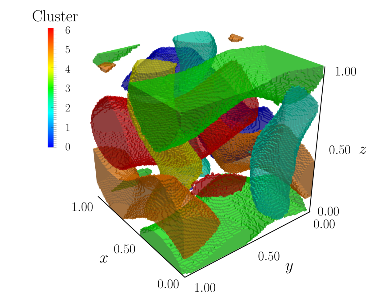
(a) Isometric view (periodicity cube rescaled to unit sides).

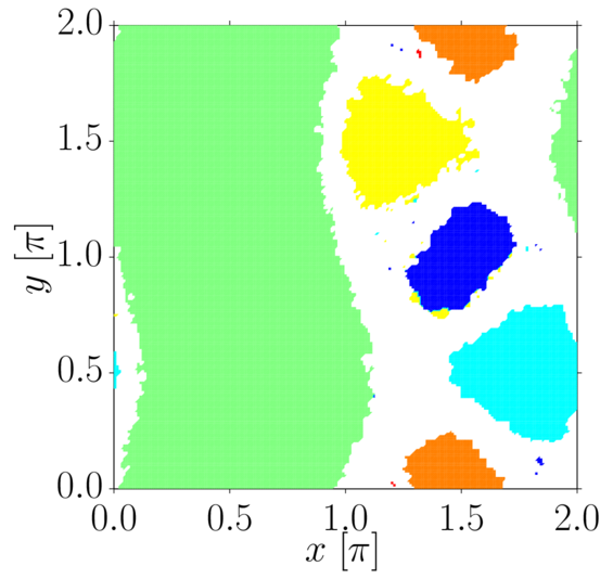
(b) Slice through $z=0$.

Figure 3. Invariant sets in the state space of the Arnold–Beltrami–Childress flow at $A=\sqrt{3},\,B=\sqrt{2},\,C=1$. Regular vortices are colored, the space between them is the chaotic zone.

To give a sense of time scales involved in the system, Figure 4 shows several trajectories (pathlines) within a single vortex, simulated for various durations $T$. Trajectories inside vortices take approximately $T=3$ to cross one periodicity cell. The two other panels in Figure 4 show that the vortex rotates around its axis while the inner layers move at slightly faster speeds than its outer layers.

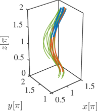
(a) Pathlines for $T=1,\,2.5,\,5$ in a periodized unit cell

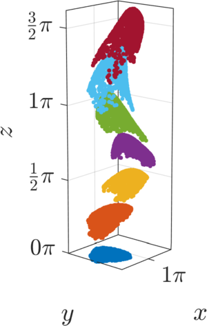
(b) Advection of points for $T=0,0.75,1.50,\dots,4.50$ (color indicates time).

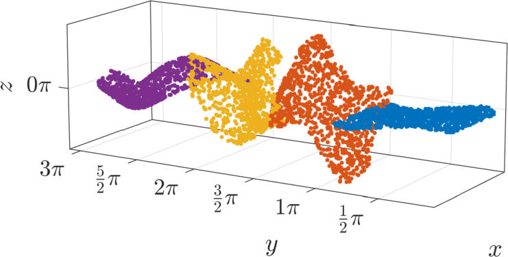
(c) Advection of points for $T=0,1.5,3.0,4.5$ (color indicates time).

Figure 4. Pathlines and advection patterns for the steady ABC flow (31) with $A=\sqrt{3},\,B=\sqrt{2},\,C=1,\,D=0$. Initial conditions clouds were sampled at $t=0$ uniformly from the $z=0$ section of the two vortices in Fig. 3(b); panel 4(b) samples the vortex centered at $x=7\pi/8,\,y=\pi/2$; panel 4(c) samples the vortex with the central axis along the line $x=\pi/2$.

To detect non-mesohyperbolic behavior we need to numerically evaluate conditions (3.3)

(35) $$t_{\psi}-t_{\psi^{-1}}=0,\quad\text{or}\quad t_{\psi}+t_{\psi^{-1}}+2=0,$$

written here using the traces of the flow map and the relation $m_{\psi}=t_{\psi^{-1}}$ to estimate their growth more clearly. These conditions are difficult to reliably compute in the face of numerical errors that will almost-certainly result in non-zero quantities.

Numerically, we determine when the criteria are satisfied using a numerical tolerance determined by estimating the growth rate of $t_{\psi}$ and $t_{\psi^{-1}}$ with increasing length $T$ of time intervals. We infer the behavior of these quantities in linear time-invariant systems in order to establish the correct baseline — the criterion has to reflect correctly our knowledge of linear systems if we are to even consider using it for classification of nonlinear systems. In what follows, we derive an empirical estimate of mesohyperbolicity, using a quantity termed numerical hyperbolicity. Our considerations will further rely on $T\to\infty$ arguments as our intent is to estimate the behavior of the flow beyond the time interval in which we are sampling it.

For a linear, time-invariant system, eigenvalues of the time-$T$ map are given either by $\pm e^{\lambda_{1}T}$, $\pm e^{\lambda_{2}T}$, $\pm e^{-(\lambda_{1}+\lambda_{2})T}$, or by $\pm e^{\lambda T\pm i\omega T}$, $\pm e^{-\lambda T}$.

In both cases, as $T\to\infty$,

(36) $$\left\lvert{t_{\psi}-t_{\psi^{-1}}}\right\rvert\sim e^{\max_{i}\lambda_{i}T},\qquad\left\lvert{t_{\psi}+t_{\psi^{-1}}+2}\right\rvert\sim e^{\max_{i}\lambda_{i}T}$$

To account for exponential growth, we set the numerical tolerance of mesohyperbolicity based on logarithms of expressions (35)

(37) $$h_{1}:=\frac{1}{T}\log\left\lvert{t_{\psi}-t_{\psi^{-1}}}\right\rvert,\qquad h_{2}:=\frac{1}{T}\log\left\lvert{t_{\psi}+t_{\psi^{-1}}+2}\right\rvert.$$

(In all expressions we omit dependence on state variables and time interval for shortness).

Non-zero values of either $h_{1}$ or $h_{2}$ are signs of mesohyperbolic behavior; conversely, we need either one of them to be small to declare non-mesohyperbolicity. In nonlinear flows, we do not expect that $h_{1,2}$ will be entirely independent of the value of $T$. Nevertheless, in ergodic regions, [67] we expect convergence in mean as $T\to\infty$.

Even the rate of convergence to the mean is not uniform: in regular ergodic regions, e.g., vortices of the ABC flow, the expected decay is $\mathcal{O}(T^{-1})$; in strongly mixing regions, conjectured to be embedded within the chaotic region, the expected decay is $\mathcal{O}(T^{-1/2})$, i.e., similar to the Central Limit Theorem for i.i.d. random variables. Initial conditions that are neither regular nor strongly mixing may potentially have an even slower decay of variance [55], $T^{-\alpha}$ for any $0<\alpha<1/2$. Values of $h$ at those points would then still grow as $h\sim T^{1/2-\alpha}$. The volume of weakly mixing zones is small in systems containing Kolmogorov–Arnold–Moser-type dynamics, [8, 54, 63] and therefore we do not expect those values to occur as major features in the histogram of $h$.

A good quantitative criterion for deciding whether a point is mesohyperbolic should estimate whether the smaller of the two $h_{1,2}$

(38) $$\max_{i}\left\lvert{\lambda_{i}}\right\rvert\sim\min\{h_{1},h_{2}\}\to 0$$

is “sufficiently” close to zero. Under a conjecture that some variant of the Central Limit Theorem (CLT) holds for the estimate of $\max_{i}\left\lvert{\lambda_{i}}\right\rvert$ we can test whether the deviation of our estimator $\min\{h_{1},h_{2}\}$ from the hypothesis of non-mesohyperbolicity $\max_{i}\left\lvert{\lambda_{i}}\right\rvert=0$ is normally distributed, i.e., whether numerical mesohyperbolicity $h$, defined by

(39) $$h =\left\lvert{\min\{h_{1},h_{2}\}}\right\rvert\sqrt{T},\ \text{where, as before}$$

$$h_{1} :=\frac{1}{T}\log\left\lvert{d_{\tilde{f}}T^{3}}\right\rvert,\qquad h_{2}:=\frac{1}{T}\log\left\lvert{8-2m_{\tilde{f}}T^{2}-3d_{\tilde{f}}T^{3}}\right\rvert$$

is small, $h<\varepsilon$, for some (small) constant $\varepsilon$. When this is indeed the case, then we are reasonably confident that with longer $T$ the estimated eigenvalues of the flow map would indeed have a unit modulus and we empirically declare that the point is not mesohyperbolic, as classified by Theorem 3.2.

Is there a fixed value of $\varepsilon$ that could help us decide whether the hypothesis of mesohyperbolicity for a point holds? To answer this question standard CLT results from probability theory, e.g., Lindeberg–Feller [14, Thm. 3.4.5], would employ higher order moments of the distribution of samples of the random processes $h_{1,2}$. Such a constant $\varepsilon$ would then turn our empirical criterion into a statistical test, where $h$ would be the z-score for testing the hypothesis of whether a point under consideration is mesohyperbolic or not. Unfortunately, we cannot assume to know how the higher moments behave, despite existing work on CLTs in the context of dynamical systems [25, 24, 57, 67, 66].

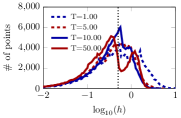
(a) Steady ABC flow

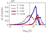
(b) Unsteady ABC flow

Figure 5. Distribution of numerical mesohyperbolicity (39) in steady and unsteady Arnold–Beltrami–Childress flows for different lengths $T$ of integration intervals, computed on a uniform grid of $400\times 400$ points. Mesohyperbolicity was declared for $h>10^{-0.3}=0.5$ (dotted vertical line).

In lieu of rigorous results, we choose to proceed empirically and set the cutoff value $\varepsilon$ based on distributions of the numerical mesohyperbolicity $h$. Figure 5(a) shows histograms of numerical mesohyperbolicity $h$ for a range of values of $T$, conforming well to expectations. As $T$ increases, the distribution of $h$ changes from a fairly flat distribution ($T=1$) to a bimodal distribution with well-separated peaks. Figure 6 shows that each mode of distribution of $h$ corresponds, respectively, to vortices and to the large chaotic region between them as $T\to\infty$. Based on these results, we declare numerical non-mesohyperbolicity using the cutoff parameter value

(40) $$h<\varepsilon,\ \text{with}\ \varepsilon=10^{-0.3}.$$

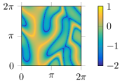
(a) $T=1$

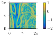
(b) $T=5$

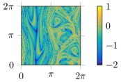
(c) $T=10$

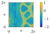
(d) $T=50$

Figure 6. Spatial distribution of numerical mesohyperbolicity on a plane in the state space of the steady Arnold–Beltrami–Childress flow. Color is $\log_{10}h$ with $h$ defined as in (39).

The Okubo–Weiss–Chong criterion requires $d_{f}\not=0$ for non-hyperbolic sets. For the given parameters at $z=0$,

$$d_{f}(x,y,z) =ABC(\cos x\cos y\cos z-\sin x\sin y\sin z)$$

$$=\sqrt{6}\cos x\cos y.$$

Therefore, a solution $\varphi(\cdot,0,p)$ with $p=(x,y,0)$ is instantaneously hyperbolic everywhere except along the lines

(41) $$x=\frac{\pi}{2},\,x=\frac{3\pi}{2},\,y=\frac{\pi}{2},\,y=\frac{3\pi}{2}.$$

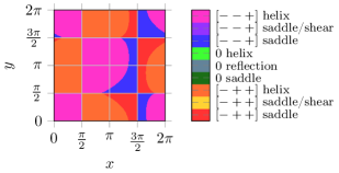
Figure 7. Mesochronic classes in the $x-y$ plane of $z=0$ slice of the Arnold–Beltrami–Childress flow state space for $T=10^{-2}$. As $T\approx 0$, the mesochronic partition is virtually identical to the Okubo–Weiss–Chong partition.

The mesochronic partition for $T\approx 0$ is illustrated in Figure 7, and due to short integration period $T$, matches exactly the Okubo–Weiss–Chong partition. Notice that the conventional intuition about vortices being “elliptic” structures cannot be inferred from short integration times, as for $T\approx 0$ almost the entire space is mesohyperbolic (non-mesohyperbolic lines (41) are difficult to sample numerically). Nevertheless, neutral mesohelical regions roughly coincide with locations of vortices, while the chaotic region between vortices contains a mixture of all four classes of mesohyperbolicity. Comparing with Figure 3, we see that the boundaries of mesochronic classes do not align with boundaries of invariant sets.

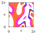
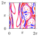
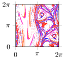
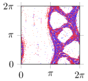
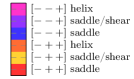
(a) Mesohyperbolic

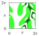
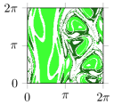
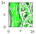
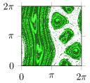
(b) Non-mesohyperbolic

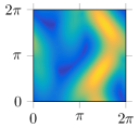
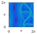
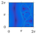
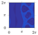
(c) FTLE

Figure 8. Distribution of mesochronic classes and the Finite-Time Lyapunov Exponents (FTLE) field on the $x-y$ plane of $z=0$ slice of the steady ABC flow for times (in rows) $T=1,\,5,\,10,\,50$.

Increasing $T$ results in the sequence of images shown in Figure 8, where the mesohyperbolic regions are shown in the left column, and the non-mesohyperbolic regions in the right column. As the averaging period is increased to $T=1$, partitions deform, but remain largely uncorrelated with invariant features. As we increase $T$ beyond $1$, non-hyperbolic behavior significantly re-appears along the interface between different mesohyperbolic classes. Parts of boundaries of mesohyperbolic zones start to align with invariant vortices. Since level sets of any function averaged for a sufficiently long time will partition the state space into invariant sets [48, 8], this is expected. Notice that the non-mesohyperbolic regions appear almost exclusively inside invariant vortices. As $T$ is increased even further, the non-mesohyperbolic zones grow inside the invariant vortices and eventually completely occupy them. In the chaotic zone, we see disappearance of mesohelical dynamics, with only saddle mesohyperbolicity remaining, which matches the asymptotic analysis in Section 4.2.

5.2.3. Unsteady case

We now keep the parameters $A=\sqrt{3},\,B=\sqrt{2},\,C=1$ as before, but set $D=1$, which results in the unsteady variation in the coefficient $A(t)=\sqrt{3}+t\sin t$. The unsteady ABC flow has not received as much analytic attention as the steady case; however, it was used as a demonstration of numerical techniques for computation of the flow map Jacobian $\nabla\psi_{T}$ in [7]. Figure 9 shows the same sets of initial conditions used in demonstrating the steady flow (Figure 4), but now advected by the unsteady flow for comparison. Notice that the initial advection patterns are similar, until $A(t)$ starts significantly deviating from its constant term $A$.

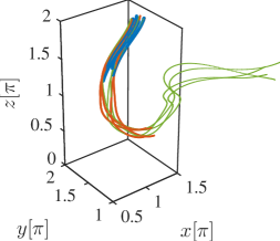
(a) Pathlines for $T=1,\,2.5,\,5$ in a periodized unit cell

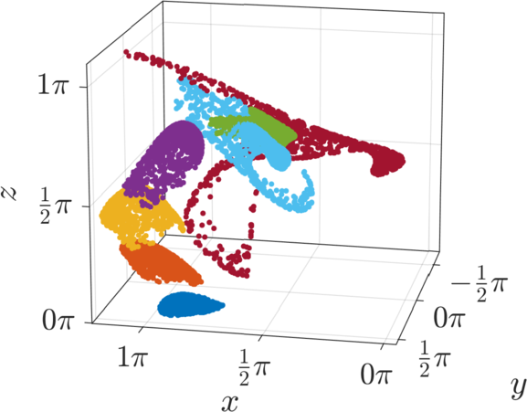
(b) Advection of points for $T=0,\,0.75,\,1.50,\dots,\,4.50$ (color indicates time).

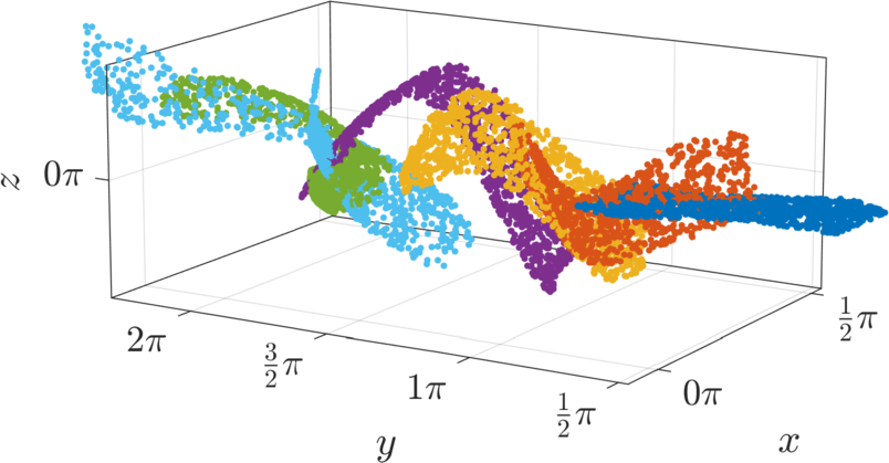
(c) Advection of points for $T=0,\,1.5,\,3.0,\,4.5$ (color indicates time).

Figure 9. Pathlines and advection patterns for the unsteady ABC flow (31) with $A=\sqrt{3},\,B=\sqrt{2},\,C=1,\,D=1$. Initial conditions clouds were sampled at $t=0$ uniformly from the $z=0$ section of the two vortices in Fig. 3(b); panel 9(b) samples the vortex centered at $x=7\pi/8,\,y=\pi/2$; panel 9(c) samples the vortex with the central axis along the line $x=\pi/2$.

Figure 5(b) shows the histogram of numerical mesohyperbolicity while Figure 10 shows the spatial distributions of (non-)mesohyperbolicity classes, determined using the same numerical criterion as in the steady case (39). For short intervals $T=0.5,\,1.0$, mesochronic classification of the flow is similar to the steady case. This is expected as the magnitude of $A(t)$ is dominated by the steady component. As time evolves, non-mesohyperbolic regions in the flow are destroyed, and the obvious split between two behaviors that was observed in the steady flow (Figure 8) is not present here. Remnants of the axial vortex in the left and two “eyes” of vortices in the right sides of images are visible both in mesochronic and FTLE partitions.

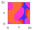
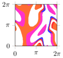
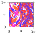
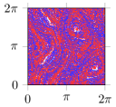
(a) Mesohyperbolic

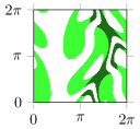
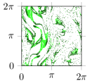
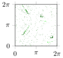
(b) Non-mesohyperbolic

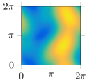
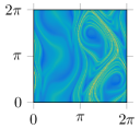
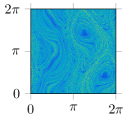
(c) FTLE

Figure 10. Distribution of mesochronic classes and the Finite-Time Lyapunov Exponents (FTLE) field on the $x-y$ plane of $z=0$ slice of the unsteady ABC flow for times (in rows) $T=1,\,5,\,10,\,50$.

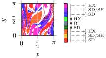
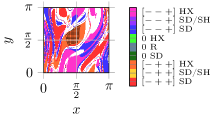
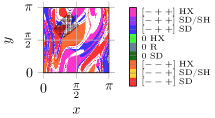
(a) Initial patch (hatched) at $t=t_{0}=0$

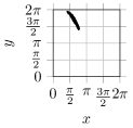
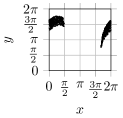
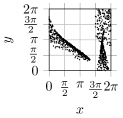
(b) Tracer at $t=5$

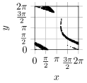
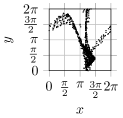
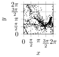
(c) Tracer at $t=7$

Figure 11. Material advection in the unsteady ABC flow. Rows show clouds of $10^{3}$ points from regions that are, respectively, mesohelical $[--+]$, $[--+]$ and mixed-mesochronic-class between $t=0$ and $t=5$. The first column shows the selection patch at time $t=0$, overlaid from the lower-left square of the third ($T=5$) panel in Fig. 10(a), with two additional times shown in the adjoining columns. Point clouds are graphed as they project onto $z=0$ plane.

Figure 11 illustrates transport of initial conditions sampled from several regions in the state space of the unsteady ABC flow. The first two rows show advection from patches chosen as subsets of regions that are mesohyperbolic for integration times $T=0.5,1,5$. The last row shows advection from a patch that straddles several mesochronic regions at $T=5$.

Advection up to $t=5$ demonstrates that the initial conditions selected from single mesochronic regions (central column, top two frames) do not disperse much, i.e., stay coherent. Initial conditions from a mixture of regions show considerably more dispersion.

Advection up to $t=7$, shown in the third column, demonstrates how the patches of initial conditions evolve beyond the interval $T=5$ that was used to generate mesochronic classes. All material patches at this point show considerable growth; arguably, the patch in the last row again shows the largest dispersion.

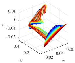
(a) $\bm{[--+]}$ mesohelical patch

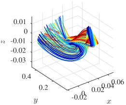
(b) $\bm{[-++]}$ mesohelical patch

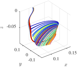
(c) $\bm{[--+]}$ mesosellar patch

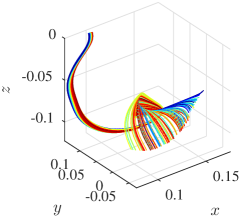
(d) $\bm{[-++]}$ mesosellar patch

Figure 12. Orbits (pathlines) of $100$ points initialized from two mesohelical patches shown in Figure 11 and two additional mesosellar patches, advected for time $t\in[0,5]$. Color is added to illustrate internal ordering of the material.

We conclude this section with Figure 12 showing images of orbits, i.e., pathlines, of material points advected by the unsteady ABC flow through space over 5 time units. Two mesohelical patches used to initialize points are the same as in Figure 11; the two additional mesosellar patches were initialized similarly. The two mesosellar sets are sampled from a narrower region, so it is not surprising that they remain more tightly packed than mesohelical sets. We believe that the major distinction between the top and the bottom row is in the internal order of orbits within each bundle. Mesohelical sets seem to preserve the internal order, i.e., despite the torsion of the bulk, one can still observe an ordered rainbow of colors toward the end of the orbits. On the other hand, both mesosellar sets show more internal mixing of colors. While this is potentially a circumstantial observation here, it may be an interesting point to explore in the future, due to the association of hyperbolic saddles with mixing and bulk rotation with lack of mixing.

6. Discussion

Mesochronic analysis is a local analysis in that it classifies a single point based on the properties of the local deformation gradients along trajectory emanating from it. Nevertheless, the hope is that sets of initial conditions selected using the local mesochronic criteria will collectively stay coherent on a macroscopic level and, potentially, deform as a bulk in the way suggested by the local analysis. The contributions of this paper are in extension of two-dimensional theory of [46] to three-dimensional flows.

We have extended the concepts of mesohyperbolicity (local strain over finite times) and mesoellipticity (local rotation over finite times) to three dimensions, which allows for co-existence of the rotation and the strain. In turn, we differentiate between the mesosellar behavior, involving three distinct directions of strain, and the mesohelical behavior, involving a plane in which material simultaneously rotates and, possibly, uniformly strains. Quantities $\Sigma$ and $\Delta$ that we defined simplify classification of domain points, side-stepping explicit calculation of eigenvalues of the flow. The eigenvectors of $\nabla\psi_{T}$ also have a role in the foregoing analysis. A complex conjugate pair determines a plane whose normal is the vector of finite-time rotation. A real eigenvector indicates the direction of finite-time stretching under the map.

Rotation of the material has a much richer presence in 3D than in 2D classification. In two dimensions, any non-uniformity in strain, accompanied by rotation or not, manifests itself as a hyperbolic deformation. In other words, only rigid-body rotations are highlighted as non-hyperbolic in two dimensions, in addition to shear. In three dimensions, rotation in a plane can be accompanied by strain in the normal direction: the type of that strain distinguishes between three mesohelical classes: $[-++],\ [--+]$ and neutral.

Consequently, the invariant vortices in the steady ABC flow initially show a significant amount of hyperbolicity in them, indicating that layers within them move at different speeds in the axial direction (Figure 4); however, over the longer timescales they appear neutrally mesohelical, which corresponds to interpretation of them as rigid rotating structures. This suggests that the separation between different layers of vortices is asymptotically sub-exponential.

In the unsteady ABC flow discussed in Section 5.2.3, material is significantly less coherent as the unsteadyness destroys long-term invariant structures. Nevertheless, for interval lengths $T=1,\ 5$, while the unsteady term $A(t)=A+Dt\sin(t)$ is of the same order of magnitude as the steady $A$, the distributions of mesohyperbolic areas show loose correspondence between steady and unsteady ABC flows. However, as $T\to 10$, the regions that turned neutrally mesohelical in the steady case are instead replaced by a mixture of hyperbolic mesosellar regions, indicative of chaotic mixing.

We have demonstrated that visualization of mesochronic classes corresponds with well-known behavior of the fluid-like ABC flow. In particular, it is interesting to see how well the mesohelical regions correspond with the vortex zones in which Kolmogorov–Arnold–Moser-type structures are known to exist. At this point, the theory is immediately applicable to kinematic analysis of the geometric structure in chaotic advection in fluids; however, numerical algorithms used in this paper serve the proof-of-concept purpose, and more accurate and efficient methods for computation of the flow Jacobian [7] can and should be readily used, if applicable.

Note that the mesochronic classification is invariant to Galilean transformations but not to rotating frame transformations [30], it therefore discovers transport properties for three-dimensional incompressible flows which are observed in the given frame of reference the system is in. It is interesting to consider the relationship between the notion of exponential dichotomy [10] and mesohyperbolicity discussed here. Mesohyperbolicity (or -ellipticity, -helicity) are notions that are valid on finite time intervals. They are best used as tools to study the bifurcations of local dynamics of a trajectory in time, when changing time intervals are selected, i.e. mesohyperbolicity is a function of two parameters, the beginning and final time. It appears plausible that, adapting the techniques used in [53], it can be shown that if a trajectory is not mesohyperbolic for any interval $[t_{1},t_{2}]$ inside the interval of interest $[T_{1},T_{2}],$ then there is no (appropriately defined [53]) finite-time exponential dichotomy on that interval. Thus, the concepts defined here have the potential to parametrize finite-time stability properties.

The true test of any method for detection of geometric structures is its usefulness to the applied communities, e.g., physical oceanography, and flow engineers. We therefore plan to apply the technique to the unsteady testbed flows in [4], to transitory systems [49] and to more physically-relevant models in order to further verify practical use of the mesochronic classification, beyond confirmations obtained for the 2D case. Furthermore, it remains to be understood if the highlighted quantities, e.g., the trace, the cofactor trace, and determinant of the mesochronic Jacobian, are also useful in dynamic analysis of turbulent fluid flows.

Appendix A Cubic polynomials and $3\times 3$ matrices

In this section we review formulas and notation for $3\times 3$ matrices. Let $A$ denote a $3\times 3$ matrix over the field $\mathbb{R}$, $A=\left[\begin{smallmatrix}a_{11}&a_{12}&a_{13}\\ a_{21}&a_{22}&a_{23}\\ a_{31}&a_{32}&a_{33}\end{smallmatrix}\right]$. The characteristic polynomial of $A$ is

(42) $$p(\lambda):=\det(\lambda\cdot\mathrm{Id}-A),$$

where $\mathrm{Id}$ is the unit matrix. The zeros of $p(\lambda)$ are the eigenvalues of $A$. Define the following quantities:

(43) $$t_{A}:= \operatorname{tr}A,\quad d_{A}:=\det A,$$

$$m_{A}:= \operatorname{tr}\operatorname{Cof}A=\det\left[\begin{smallmatrix}a_{11}&a_{12}\\ a_{21}&a_{22}\end{smallmatrix}\right]$$

$$+\det\left[\begin{smallmatrix}a_{11}&a_{13}\\ a_{31}&a_{33}\end{smallmatrix}\right]+\det\left[\begin{smallmatrix}a_{22}&a_{23}\\ a_{32}&a_{33}\end{smallmatrix}\right],$$

where $\operatorname{Cof}A$ is the cofactor matrix of $A$, containing signed minors. By expanding equation (42) we can verify that

(44) $$p(\lambda)=\lambda^{3}-t_{A}\lambda^{2}+m_{A}\lambda-d_{A}.$$

For a polynomial with real coefficients, the zeros $\lambda_{1},\lambda_{2},\lambda_{3}$ are either all real, or two of them appear as a complex conjugate pair, in which case we denote them by $\lambda_{r},\lambda_{c},\bar{\lambda}_{c}$. By convention, we will assume that the imaginary part $\Im\lambda_{c}>0$.

The discriminant of a cubic polynomial $f(\lambda)=\lambda^{3}+f_{2}\lambda^{2}+f_{1}\lambda+f_{0}$ is given by

$$\mathcal{D}(f):= \ 18f_{2}f_{1}f_{0}-4f_{2}^{3}f_{0}+f_{2}^{2}f_{1}^{2}$$

$$-4f_{1}^{3}-27f_{0}^{2},$$

its sign determines whether the zeros of $f$ lie on the real axis or not (see Ref. [22], §12.1.B).

Using the notation from (44), we see that $f_{2}=-t_{A}$, $f_{1}=m_{A}$, $f_{0}=d_{A}$, therefore

$$\mathcal{D}(p)= 18t_{A}m_{A}d_{A}-4t_{A}^{3}d_{A}$$

$$+t_{A}^{2}m_{A}^{2}-4m_{A}^{3}-27d_{A}^{2}.$$

It then holds (see Ref. [34], §10.3, Ex. 10.14) that:

• $\mathcal{D}(p)>0$, the zeros are $\lambda_{1},\lambda_{2},\lambda_{3}\in\mathbb{R}$,

• $\mathcal{D}(p)=0$, the zeros are $\lambda_{1},\lambda_{2}=\lambda_{3}\in\mathbb{R}$,

• $\mathcal{D}(p)<0$, the zeros are $\lambda_{r}\in\mathbb{R}$, $\lambda_{c},\bar{\lambda}_{c}\in\mathbb{C}$.

The following also holds in general for eigenvalues $\lambda_{1,2,3}\in\mathbb{C}$, which can be seen by expanding $(\lambda-\lambda_{1})(\lambda-\lambda_{2})(\lambda-\lambda_{3})$ and comparing to (44):

$$d_{A}= \ \det A=\lambda_{1}\lambda_{2}\lambda_{3},$$

$$m_{A}= \ \operatorname{tr}\operatorname{Cof}A=\lambda_{1}\lambda_{2}+\lambda_{1}\lambda_{3}+\lambda_{2}\lambda_{3},$$

$$t_{A}= \ \operatorname{tr}A=\lambda_{1}+\lambda_{2}+\lambda_{3}.$$

Appendix B Differential equation for the mesochronic Jacobian

If an initial condition $x\in\mathbb{R}$ and initial time $t_{0}$ are fixed, the mesochronic Jacobian matrix $\nabla\tilde{f}_{\tau}(x)$ satisfies a matrix-valued ODE in the variable $\tau$, the length of the averaging interval. To evaluate the mesochronic Jacobian for the purposes of classifying $(t_{0},x)$ into one of the classes described in Section 3, we numerically solve a particular matrix-valued initial value problem and evaluate its solution at $\tau=T$.

To derive the ODE for the mesochronic Jacobian, start from the integral expression for the time-$\tau$ map and compute its Jacobian:

$$\psi_{\tau}(x)=x+\int_{t_{0}}^{t_{0}+\tau}f(t_{0}+t,\psi_{t}(x))dt$$

$$\nabla\psi_{\tau}(x)=\mathrm{Id}+\int_{t_{0}}^{t_{0}+\tau}\nabla f(t_{0}+t,\psi_{t}(x))\cdot\nabla\psi_{t}(x)dt$$

$$\nabla\psi_{\tau}^{\prime}(x)=\nabla f(t_{0}+\tau,\psi_{\tau}(x))\cdot\nabla\psi_{\tau}(x),$$

where ^′ denotes $d/d\tau$.

We now substitute relation (13), $\nabla\psi_{\tau}(x)=\mathrm{Id}+\tau\nabla\tilde{f}_{\tau}(x)$, linking the time-$\tau$ map $\psi_{\tau}$ and the mesochronic Jacobian $\nabla\tilde{f}_{\tau}$. To simplify notation, we use $M(\tau):=\nabla\tilde{f}_{\tau}(x)$ and $A(\tau):=\nabla f(t_{0}+\tau,\psi_{\tau}(x))$ for the mesochronic and advected velocity field Jacobian, respectively.

(45) $$\left(\mathrm{Id}+\tau M(\tau)\right)^{\prime}=A(\tau)\cdot\left(\mathrm{Id}+\tau M(\tau)\right)$$

$$M(\tau)+\tau\dot{M}(\tau)=A(\tau)+\tau A(\tau)\cdot M(\tau)$$

$$\dot{M}(\tau)=\big{(}A(\tau)-M(\tau)\big{)}/\tau+A(\tau)\cdot M(\tau).$$

The initial condition for the matrix ODE is set at $\tau=0$ when the mesochronic Jacobian $\nabla\tilde{f}_{\tau}(x)$ is identical to the velocity field Jacobian $\nabla\tilde{f}_{0}(x)=\nabla f(t_{0},x),$ therefore

(46) $$M(0)=A(0)\quad\text{and}\quad\dot{M}(0)={A(0)}^{2},$$

where the last calculation is obtained from (45) by evaluating the first-order expansion of $A(\tau)-M(\tau)$ at $\tau=0$.

Appendix C Implementation of the mesochronic classification

In what follows we provide the basic algorithm which we used to produce a numerical implementation of mesochronic classification, used to generate images analogous to Figures 8, and 10. The core task is to assign a mesochronic class (Definition 2.4), corresponding to the time interval $[t_{0},t_{0}+T]$, to a fixed initial condition $x\in\mathbb{R}^{3}$.

This task can be split into the following sequence of stages.

1. Compute the trajectory segment $x(t)$ for $t\in[t_{0},t_{0}+T]$ where $x(t_{0})=x$.

2. Evaluate the Jacobian matrix $A(\tau):=\nabla f(t_{0}+\tau,x(t_{0}+\tau))$ of the velocity field along the trajectory $x(t)$.

3. Evaluate the mesochronic Jacobian matrix $\nabla\tilde{f}_{\tau}$ at the endpoint $\tau=T$ by integrating the initial value problem given by (45) and (46):

   $$\dot{M}(\tau) =\big{(}A(\tau)-M(\tau)\big{)}/\tau+A(\tau)\cdot M(\tau),$$

   $$M(0) =A(0),\ \dot{M}(0)=A{(0)}^{2}.$$

4. Compute the determinant $d_{\tilde{f}}=\det M(T)$, cofactor trace $m_{\tilde{f}}=\operatorname{tr}\operatorname{Cof}M(T)$, evaluate $\Delta$ and $\Sigma$, (14).

5. Based on the signs of $\Delta$ and $\Sigma$ assign the mesochronic class to the pair of initial condition and time interval $(p,[t_{0},t_{0}+T])$ using Theorem 3.2.

Remark to Step (1).

We assume that the velocity field $f(t,x)$ can be evaluated on the entire domain of interest and throughout the entire compact time interval $I\in\mathbb{R}$. If the velocity field is known only on a grid of points $(t,x)$, then interpolation of the velocity field is likely needed.

Remark to Step (2).

We assume the knowledge of the Jacobian matrix of the vector field evaluated along the trajectory segment $[t_{0},t_{0}+\tau]$, termed $A(\tau):=\nabla f(t_{0}+\tau,x(t_{0}+\tau))$. If the velocity field was known analytically, it might be possible to express $\nabla f$ analytically as well and evaluate it along points computed in Step 1. If not, $\nabla f$ can be numerically approximated using a central spatial-difference scheme with a spatial step $\delta$. On finite-precision computers, $\delta$ cannot be taken arbitrarily small, due to finite-precision effects. There will always exist an optimal, non-zero $\delta$, which depends on the machine precision and magnitude of higher derivatives of $f$ (see Ref. [50], §8).

Remark to Step (3).

Equation (45) is a linear, matrix-valued ODE where the vector field Jacobian $A(t)$, computed in Step 2, comes in as both inhomogeneity and as the parametric term. This ODE can be discretized using one of the standard time-stepping schemes, on the same time points used for discretization of $x(t)$ in Step (1). The examples in this paper were computed using an explicit Adams–Bashforth stepping scheme with a fixed time step.

Since each of the presented steps involves some degree of numerical approximation, the mesochronic Jacobian $M(T)$ will contain numerical noise. As the derivation of the mesochronic classification criteria hinges on the assumption of incompressibility of the flow, i.e., (9), the necessary criterion for accuracy of the numerical approximation is that the numerical compressibility $\operatorname{tr}M(\tau)+\tau\cdot\operatorname{tr}\operatorname{Cof}M(\tau)+\tau^{2}\det M(\tau)\approx 0$. If the numerical compressibility is significantly larger than $0$ when evaluated using numerical $M(\tau)$, this can be taken as an indication of significant numerical errors in the mesochronic Jacobian and, consequently, in mesochronic classification.

References

- [1] L. Y. Adrianova, Introduction to linear systems of differential equations, vol. 146 of Translations of Mathematical Monographs, American Mathematical Society, Providence, RI, 1995.
- [2] M. Allshouse and J.-L. Thiffeault, Detecting coherent structures using braids, Physica D. Nonlinear Phenomena, 95–105.
- [3] H. Aref and E. P. Flinchem, Dynamics of a Vortex Filament in a Shear-Flow, Journal of Fluid Mechanics, 148 (1984), 477–497.
- [4] S. Balasuriya, Explicit invariant manifolds and specialised trajectories in a class of unsteady flows, Physics of Fluids (1994-present), 24 (2012), 127101.
- [5] D. Blazevski and G. Haller, Hyperbolic and elliptic transport barriers in three-dimensional unsteady flows, Physica D: Nonlinear Phenomena, 273–274 (2014), 46–62.
- [6] P. L. Boyland, H. Aref and M. A. Stremler, Topological fluid mechanics of stirring, Journal of Fluid Mechanics, 403 (2000), 277–304.
- [7] S. L. Brunton and C. W. Rowley, Fast computation of finite-time Lyapunov exponent fields for unsteady flows, Chaos: An Interdisciplinary Journal of Nonlinear Science, 20 (2010), 017503.
- [8] M. Budišić and I. Mezić, Geometry of the ergodic quotient reveals coherent structures in flows, Physica D. Nonlinear Phenomena, 241 (2012), 1255–1269.
- [9] M. S. Chong, A. E. Perry and B. J. Cantwell, A general classification of three-dimensional flow fields, Physics of Fluids A: Fluid Dynamics (1989-1993), 2 (1990), 765–777.
- [10] W. A. Coppel, Dichotomies in stability theory, Lecture Notes in Mathematics, Vol. 629, Springer-Verlag, Berlin-New York, 1978.
- [11] M. Dellnitz and O. Junge, On the approximation of complicated dynamical behavior, SIAM Journal on Numerical Analysis, 36 (1999), 491–515.
- [12] M. Dellnitz and O. Junge, Set oriented numerical methods for dynamical systems, in Handbook of dynamical systems, Vol. 2, North-Holland, Amsterdam, 2002, 221–264.
- [13] T. Dombre, U. Frisch, J. M. Greene, M. Hénon, A. Mehr and A. M. Soward, Chaotic streamlines in the ABC flows, Journal of Fluid Mechanics, 167 (1986), 353–391.
- [14] R. Durrett, Probability: theory and examples, 4th edition, Cambridge Series in Statistical and Probabilistic Mathematics, Cambridge University Press, Cambridge, 2010.
- [15] M. Farazmand, Hyperbolic Lagrangian coherent structures align with contours of path-averaged scalars, arXiv:1501.05036 [nlin, physics:physics].
- [16] M. Farazmand and G. Haller, Polar rotation angle identifies elliptic islands in unsteady dynamical systems, Physica D: Nonlinear Phenomena, 315 (2016), 1–12.
- [17] A. M. Fox and J. D. Meiss, Greene’s residue criterion for the breakup of invariant tori of volume-preserving maps, Physica D: Nonlinear Phenomena, 243 (2013), 45–63.
- [18] G. Froyland and M. Dellnitz, Detecting and locating near-optimal almost-invariant sets and cycles, SIAM Journal on Scientific Computing, 24 (2003), 1839–1863 (electronic).
- [19] G. Froyland, S. Lloyd and N. Santitissadeekorn, Coherent sets for nonautonomous dynamical systems, Physica D: Nonlinear Phenomena, 239 (2010), 1527–1541.
- [20] G. Froyland and K. Padberg, Almost-invariant sets and invariant manifolds—connecting probabilistic and geometric descriptions of coherent structures in flows, Physica D. Nonlinear Phenomena, 238 (2009), 1507–1523.
- [21] G. Froyland, N. Santitissadeekorn and A. Monahan, Transport in time-dependent dynamical systems: Finite-time coherent sets, Chaos: An Interdisciplinary Journal of Nonlinear Science, 20 (2010), 043116.
- [22] I. M. Gelfand, M. M. Kapranov and A. V. Zelevinsky, Discriminants, resultants and multidimensional determinants, Modern Birkhäuser Classics, Birkhäuser Boston Inc., Boston, MA, 2008.
- [23] I. Goldhirsch, P.-L. Sulem and S. A. Orszag, Stability and Lyapunov stability of dynamical systems: A differential approach and a numerical method, Physica D: Nonlinear Phenomena, 27 (1987), 311–337.
- [24] S. Gouëzel, Central limit theorem and stable laws for intermittent maps, Probability Theory and Related Fields, 128 (2004), 82–122.
- [25] S. Gouëzel and I. Melbourne, Moment bounds and concentration inequalities for slowly mixing dynamical systems, Electronic Journal of Probability, 19 (2014), no. 93, 30.
- [26] J. M. Greene, Two-dimensional measure-preserving mappings, Journal of Mathematical Physics, 9 (1968), 760–768.
- [27] J. M. Greene, Method for Determining a Stochastic Transition, Journal of Mathematical Physics, 20 (1979), 1183–1201.
- [28] G. Haller, Lagrangian structures and the rate of strain in a partition of two-dimensional turbulence, Physics of Fluids, 13 (2001), 3365–3385.
- [29] G. Haller, A variational theory of hyperbolic Lagrangian Coherent Structures, Physica D. Nonlinear Phenomena, 240 (2011), 574–598.
- [30] G. Haller, Lagrangian Coherent Structures, Annual Review of Fluid Mechanics, 47 (2015), 137–162.
- [31] G. Haller and F. J. Beron-Vera, Geodesic theory of transport barriers in two-dimensional flows, Physica D: Nonlinear Phenomena, 241 (2012), 1680–1702.
- [32] G. Haller and A. C. Poje, Finite time transport in aperiodic flows, Physica D. Nonlinear Phenomena, 119 (1998), 352–380.
- [33] G. Haller and G. Yuan, Lagrangian coherent structures and mixing in two-dimensional turbulence, Physica D. Nonlinear Phenomena, 147 (2000), 352–370.
- [34] R. S. Irving, Integers, polynomials, and rings, Undergraduate Texts in Mathematics, Springer-Verlag, New York, 2004.
- [35] B. O. Koopman, Hamiltonian Systems and Transformations in Hilbert Space, Proceedings of National Academy of Sciences, 17 (1931), 315–318.
- [36] Z. Levnajić and I. Mezić, Ergodic theory and visualization. I. Mesochronic plots for visualization of ergodic partition and invariant sets, Chaos: An Interdisciplinary Journal of Nonlinear Science, 20 (2010), –.
- [37] T. Ma and E. M. Bollt, Differential Geometry Perspective of Shape Coherence and Curvature Evolution by Finite-Time Nonhyperbolic Splitting, SIAM Journal on Applied Dynamical Systems, 13 (2014), 1106–1136.
- [38] T. Ma and E. M. Bollt, Shape Coherence and Finite-Time Curvature Evolution, International Journal of Bifurcation and Chaos, 25 (2015), 1550076.
- [39] T. Ma, N. T. Ouellette and E. M. Bollt, Stretching and folding in finite time, Chaos: An Interdisciplinary Journal of Nonlinear Science, 26 (2016), 023112.
- [40] J. A. J. Madrid and A. M. Mancho, Distinguished trajectories in time dependent vector fields, Chaos: An Interdisciplinary Journal of Nonlinear Science, 19 (2009), 013111.
- [41] N. Malhotra, I. Mezić and S. Wiggins, Patchiness: A New Diagnostic for Lagrangian Trajectory Analysis in Time-Dependent Fluid Flows, International Journal of Bifurcation and Chaos, 08 (1998), 1053–1093.
- [42] A. M. Mancho, S. Wiggins, J. Curbelo and C. Mendoza, Lagrangian descriptors: A method for revealing phase space structures of general time dependent dynamical systems, Communications in Nonlinear Science and Numerical Simulation, 18 (2013), 3530–3557.
- [43] I. Mezić, On the geometrical and statistical properties of dynamical systems: theory and applications, Phd thesis, California Institute of Technology, 1994.
- [44] I. Mezić, Spectral properties of dynamical systems, model reduction and decompositions, Nonlinear Dynamics. An International Journal of Nonlinear Dynamics and Chaos in Engineering Systems, 41 (2005), 309–325.
- [45] I. Mezić and A. Banaszuk, Comparison of systems with complex behavior, Physica D. Nonlinear Phenomena, 197 (2004), 101–133.
- [46] I. Mezić, S. Loire, V. A. Fonoberov and P. J. Hogan, A New Mixing Diagnostic and Gulf Oil Spill Movement, Science Magazine, 330 (2010), 486–489.
- [47] I. Mezić and F. Sotiropoulos, Ergodic theory and experimental visualization of invariant sets in chaotically advected flows, Physics of Fluids, 14 (2002), 2235.
- [48] I. Mezić and S. Wiggins, A method for visualization of invariant sets of dynamical systems based on the ergodic partition, Chaos: An Interdisciplinary Journal of Nonlinear Science, 9 (1999), 213–218.
- [49] B. A. Mosovsky and J. D. Meiss, Transport in transitory dynamical systems, SIAM Journal on Applied Dynamical Systems, 10 (2011), 35–65.
- [50] J. Nocedal and S. J. Wright, Numerical optimization, 2nd edition, Springer Series in Operations Research and Financial Engineering, Springer, New York, 2006.
- [51] A. Okubo, Horizontal Dispersion of Floatable Particles in Vicinity of Velocity Singularities Such as Convergences, Deep-Sea Research, 17 (1970), 445–454.
- [52] J. M. Ottino, The kinematics of mixing: stretching, chaos, and transport, Cambridge Texts in Applied Mathematics, Cambridge University Press, Cambridge, 1989.
- [53] K. J. Palmer, A finite-time condition for exponential dichotomy, Journal of Difference Equations and Applications, 17 (2011), 221–234.
- [54] A. D. Perry and S. Wiggins, KAM tori are very sticky: rigorous lower bounds on the time to move away from an invariant Lagrangian torus with linear flow, Physica D. Nonlinear Phenomena, 71 (1994), 102–121.
- [55] K. Petersen, Ergodic theory, vol. 2 of Cambridge Studies in Advanced Mathematics, Cambridge University Press, Cambridge, UK, 1989.
- [56] A. Poje, G. Haller and I. Mezić, The geometry and statistics of mixing in aperiodic flows, Physics of Fluids, 11 (1999), 2963–2968.
- [57] L. Rey-Bellet and L.-S. Young, Large deviations in non-uniformly hyperbolic dynamical systems, Ergodic Theory and Dynamical Systems, 28 (2008), 587–612.
- [58] D. P. Ruelle, Rotation numbers for diffeomorphisms and flows, Annales de l’Institut Henri Poincaré. Physique Théorique, 42 (1985), 109–115.
- [59] R. M. Samelson, Lagrangian Motion, Coherent Structures, and Lines of Persistent Material Strain, Annual Review of Marine Science, 5 (2013), 137–163.
- [60] S. C. Shadden, F. Lekien and J. E. Marsden, Definition and properties of Lagrangian coherent structures from finite-time Lyapunov exponents in two-dimensional aperiodic flows, Physica D. Nonlinear Phenomena, 212 (2005), 271–304.
- [61] J. D. Szezech Jr., A. B. Schelin, I. L. Caldas, S. R. Lopes, P. J. Morrison and R. L. Viana, Finite-time rotation number: A fast indicator for chaotic dynamical structures, Physics Letters A, 377 (2013), 452–456.
- [62] J.-L. Thiffeault, Braids of entangled particle trajectories, Chaos: An Interdisciplinary Journal of Nonlinear Science, 20 (2010), 017516–017514.
- [63] D. Treschev, Width of stochastic layers in near-integrable two-dimensional symplectic maps, Physica D. Nonlinear Phenomena, 116 (1998), 21–43.
- [64] J. Weiss, The dynamics of enstrophy transfer in two-dimensional hydrodynamics, Physica D. Nonlinear Phenomena, 48 (1991), 273–294.
- [65] S. Wiggins, Chaotic transport in dynamical systems, vol. 2 of Interdisciplinary Applied Mathematics, Springer-Verlag, New York, 1992.
- [66] L.-S. Young, Some Large Deviation Results for Dynamical Systems, Transactions of the American Mathematical Society, 318 (1990), 525–543.
- [67] L.-S. Young, Statistical Properties of Dynamical Systems with Some Hyperbolicity, Annals of Mathematics, 147 (1998), 585–650.