Consequences of viscous anisotropy in a deforming, two-phase aggregate. Why is porosity-band angle lowered by viscous anisotropy?

Abstract

In laboratory experiments that impose shear deformation on partially molten aggregates of initially uniform porosity, melt segregates into high-porosity sheets (bands in cross-section). The bands emerge at $15$–$20^{\circ}$ to the shear plane. A model of viscous anisotropy can explain these low angles whereas previous, simpler models have failed to do so. The anisotropic model is complex, however, and the reason that it produces low-angle bands has not been understood. Here we show that there are two mechanisms: (i) suppression of the well-known tensile instability, and (ii) creation of a new, shear-driven instability. We elucidate these mechanisms using linearised stability analysis in a coordinate system that is aligned with the perturbations. We consider the general case of anisotropy that varies dynamically with deviatoric stress, but approach it by first considering uniform anisotropy that is imposed a priori and showing the difference between static and dynamic cases. We extend the model of viscous anisotropy to include a strengthening in the direction of maximum compressive stress. Our results support the hypothesis that viscous anisotropy is the cause of low band-angles in experiments.

1 Introduction

In laboratory experiments, forced shear deformation of nominally uniform, partially molten rocks causes melt segregation into high-porosity bands oriented at low angle ($15$–$20^{\circ}$) to the shear plane (Holtzman et al., 2003; Holtzman and Kohlstedt, 2007; King et al., 2010). Stevenson (1989) predicted the emergence of such bands in a self-reinforcing feedback arising from the porosity-weakening of the crystal$+$magma aggregate, but the angle predicted by this theory was $45^{\circ}$ (Spiegelman, 2003), much higher than observed. The low angle of high-porosity bands is widely thought to provide an additional constraint on the rheology of the aggregate, but it has proven challenging to understand. Katz et al. (2006) found that non-Newtonian viscosity with a high sensitivity to stress could reproduce the low angle of bands, but King et al. (2010) subsequently showed that the viscosity of experiments that produce low-angle bands is actually close to Newtonian.

Theory by Takei and Holtzman (2009a, b) of anisotropic viscosity under diffusion creep of a partially molten aggregate represents a possible solution. This theory is motivated by observations of the coherent alignment of melt-pockets between solid grains under a deviatoric stress (e.g. Daines and Kohlstedt, 1997; Zimmerman et al., 1999) and of the enhancement of diffusion creep by melt at grain boundaries and triple junctions (e.g. Cooper et al., 1989). The melt is a fast pathways for diffusional transport of solid constituents around grains; the alignment of melt with respect to the principal-stress directions hypothetically results in anisotropic viscosity of the aggregate (Takei and Holtzman, 2009a).

Analysis of the theory of anisotropic viscosity by Takei and Holtzman (2009b), Takei and Katz (2013), Katz and Takei (2013), and Allwright and Katz (2014) shows that it introduces qualitatively different behaviour from previous models with isotropic (and even power-law) viscosity. Shear and normal components of stress and strain-rate are coupled under viscous anisotropy; as a result of this coupling, a gradient in shear stress becomes a driving force for melt segregation that is not present in the isotropic system. Under Poiseuille flow, melt segregates toward higher-stress regions; under torsional flow, compressive hoop stresses drive the solid outward and the magma inward. The mechanics of this “base-state” melt segregation are explained in detail by Takei and Katz (2013). An experimental test of radial melt segregation in torsional flow by Qi et al. (2015) shows striking consistency with predictions.

Furthermore, theoretical work has demonstrated that there is a connection between the strength of anisotropy and the angle of high-porosity bands that emerge by unstable growth. This was shown with linearised stability analysis (Takei and Holtzman, 2009b; Takei and Katz, 2013) and numerical simulations (Butler, 2012; Katz and Takei, 2013) where the strength and orientation of anisotropy are assumed to be known and are imposed a priori. In those static-anisotropy calculations, high-porosity bands emerge at low angles to the shear plane only when viscous anisotropy is at or near saturation. This is a rather restrictive condition that may be incompatible with the robust appearance and consistently low angle of bands in experiments (Holtzman and Kohlstedt, 2007). However, in numerical simulations that allow anisotropy strength and direction to vary dynamically in space and time (Katz and Takei, 2013), band angles are significantly lowered and appear to be less sensitive to the mean strength of anisotropy. These findings raise several basic, unanswered questions: Why do the mechanics of viscous anisotropy give rise to low-angle bands? Why is dynamic anisotropy more effective in this regard than static anisotropy? What are the general conditions under which low-angle, high-porosity bands should form?

The present manuscript addresses these questions through a combination of linearised stability analysis and physical reasoning. The crucial, enabling advance is to perform the analysis in a coordinate system that is rotated to align with the porosity bands (rather than with the plane of shear). This drastically simplifies the expressions for growth rate under static anisotropy (Takei and Katz, 2013), making them readily interpretable in physical terms. Moreover, it allows us to extend the analysis to dynamic anisotropy in a form that exposes the physical differences from static anisotropy. Finally, the same coordinate rotation clarifies the physical reason for low angles under isotropic, non-Newtonian viscosity.

The manuscript is organised as follows. In the next section, we briefly discuss the nondimensionalised governing equations and present an anisotropic, viscous constitutive model for the two-phase, partially molten aggregate. The full, non-linear system is solved numerically in §3 for static and dynamic cases, to elucidate the questions listed above. The coordinate rotation is introduced and the linearised stability analysis is developed in §4. In particular, §4.3 develops an expression for the growth-rate of porosity perturbations under the fully dynamic model of §2. This expression is challenging to understand and so we subsequently consider it under reducing assumptions of static anisotropy (§5.1), which includes the simplest case of Newtonian, isotropic model. We build on this to explain the full complexity in §5.2 and §5.3. We conclude with a summary and discussion of the results in terms of the motivating questions.

2 Governing and constitutive equations

In the theory of magma/mantle interaction, the macroscopic behaviour of a two-phase aggregate is treated within the framework of continuum mechanics (e.g. Drew, 1983; McKenzie, 1984). This theory is concerned with the evolution of macroscopic fields including the volume fraction of melt or porosity $\phi$, the velocity of the solid phase $\mathbf{V}$, the liquid pressure $P$ (compression positive), and the bulk or phase-averaged stress tensor $\sigma_{ij}=(1-\phi)\sigma^{S}_{ij}-\phi P\delta_{ij}$ where $\sigma^{S}_{ij}$ is the stress tensor of the solid phase (tension positive). Further details of the two-phase-flow theory were previously presented (e.g. Takei and Katz, 2013; Rudge et al., 2011) and are not repeated here.

We proceed directly to the nondimensional governing equations,

$$\frac{\partial{\phi}}{\partial{t}} =\mbox{\boldmath$\nabla$}\!\cdot\left[(1-\phi){\bf V}\right],$$ (1a)

$$\mbox{\boldmath$\nabla$}\!\cdot{\bf V} =\frac{R^{2}}{r_{\xi}+4/3}\mbox{\boldmath$\nabla$}\!\cdot\left[\left(\frac{\phi}{\phi_{0}}\right)^{\ell}\mbox{\boldmath$\nabla$}P\right],$$ (1b)

$$\mbox{\boldmath$\nabla$}P =\mbox{\boldmath$\nabla$}\!\cdot\boldsymbol{\tau},$$ (1c)

and refer the reader to Takei and Katz (2013) and references therein for details of the derivation and rescaling. In the system (1) we have introduced the differential stress tensor $\tau_{ij}\equiv\sigma_{ij}+P\delta_{ij}$. Also, we have excluded body forces and assumed that the permeability of the solid matrix is a function of the porosity only, proportional to $(\phi/\phi_{0})^{\ell}$, where $\phi_{0}$ is a reference porosity and $\ell$ is a constant. $R$ is the nondimensional compaction length and $r_{\xi}$ is a rheological parameter explained below. To close the system, a constitutive relationship that relates the differential stress $\tau_{ij}$ and strain rate $\dot{e}_{ij}=(V_{i,j}+V_{j,i})/2$ is required.

Takei and Holtzman (2009b) and Takei and Katz (2013) proposed a model of anisotropic viscosity caused by stress-induced microstructural anisotropy. In partially molten rocks, the melt phase is contained within a permeable network of tubules between grains. The solid matrix is formed by a contiguous skeleton of solid grains. The area of grain-to-grain contact is known as the contiguity. Contiguity is the microstructural variable that determines the macroscopic (i.e., continuum) mechanical properties of the matrix (Takei, 1998; Takei and Holtzman, 2009a). Although the equilibrium microstructure developed under hydrostatic stress has isotropic contiguity, deviations from the equilibrium microstructure have been observed in experimentally deformed, partially molten samples (e.g. Daines and Kohlstedt, 1997; Takei, 2010). Based on these observations, we infer that under a differential stress, the grain-to-grain contacts with normals that are parallel to the maximum tensile stress ($\tau_{3}$) are reduced in area; similarly, the areas of those with normals parallel to the maximum compressive stress ($\tau_{1}$) are increased. Using a microstructure-based model of aggregate viscosity (Takei and Holtzman, 2009a) and a coordinate transformation (Takei and Katz, 2013), the constitutive law and the viscosity tensor are

$$\tau_{ij}=C_{ijkl}\dot{e}_{kl},$$ (2a)

$$C_{ijkl}=\textrm{e}^{-\lambda(\phi-\phi_{0})}\times\\ \bordermatrix{ij\!\downarrow&kl\!\rightarrow XX&YY&XY\\[2.84526pt] XX&r_{\xi}+\frac{4}{3}-\frac{\alpha+\beta}{2}\cos 2\Theta&r_{\xi}-\frac{2}{3}&-\frac{\alpha+\beta}{4}\sin 2\Theta\\[-2.84526pt] &-\frac{\alpha-\beta}{8}(3+\cos 4\Theta)&-\frac{\alpha-\beta}{8}(1-\cos 4\Theta)&-\frac{\alpha-\beta}{8}\sin 4\Theta\\[5.69054pt] YY&\cdot&r_{\xi}+\frac{4}{3}+\frac{\alpha+\beta}{2}\cos 2\Theta&-\frac{\alpha+\beta}{4}\sin 2\Theta\\[-2.84526pt] &&-\frac{\alpha-\beta}{8}(3+\cos 4\Theta)&+\frac{\alpha-\beta}{8}\sin 4\Theta\\[5.69054pt] XY&\cdot&\cdot&1-\frac{\alpha-\beta}{8}(1-\cos 4\Theta)}.$$ (2b)

For simplicity, we consider a two dimensional problem, in which the $\tau_{1}$–$\tau_{3}$ plane is parallel to the $X$–$Y$ plane. Therefore only the two-dimensional version of $C_{ijkl}$ is written in (2b). Only 6 of the 16 components are shown due to the symmetry of $C_{ijkl}$ under the exchange of $i$ and $j$, $k$ and $l$, and $ij$ and $kl$.

The factor in front of the matrix represents the normalised shear viscosity $\eta(\phi)/\eta(\phi_{0})$; it decreases exponentially with increasing melt fraction $\phi$, and so $\lambda$ is called the porosity-weakening factor. We take $\lambda=27$ based on the experimental results (e.g. Mei et al., 2002). The parameter $r_{\xi}$ represents the bulk-to-shear viscosity ratio, $r_{\xi}=\xi/\eta$, which is assumed to be constant (=5/3) based on theoretical results by Takei and Holtzman (2009a) (although see Simpson et al., 2010a, b). Parameters $\alpha$, $\beta$, and $\Theta$ represent the magnitude and direction of microstructural anisotropy: $\alpha$ and $\beta$ quantify the amplitude of contiguity reduction and increase, respectively, in the directions of principal stress $\tau_{3}$ and $\tau_{1}$; $\Theta$ represents the angle that the most-tensile stress ($\tau_{3}$) direction makes with the $X$-axis of the coordinate system. Using the local differential stress $\tau_{ij}$, $\Theta$ is given by

$$\tan 2\Theta=\frac{2\tau_{XY}}{\tau_{XX}-\tau_{YY}},$$ (3)

and $\alpha$ and $\beta$ are modelled as

$$\alpha =1+\tanh\displaystyle\left(\frac{2(\Delta\tau-\tau_{\textrm{offset}})}{\tau_{\textrm{sat}}}\right),$$ (4a)

$$\beta =r_{\beta}\alpha,$$ (4b)

where $\Delta\tau$ $=\tau_{3}-\tau_{1}$ $=\sqrt{(\tau_{XX}-\tau_{YY})^{2}+4\tau_{XY}^{2}}$ represents the amplitude of deviatoric stress. The detailed forms of the functions in (4) are poorly constrained, owing to a lack of experimental data. The form of $\alpha$ was chosen based on the constraints that $\alpha$ is less than or equal to 2 (Takei and Katz, 2013) and increases with increasing differential stress (Daines and Kohlstedt, 1997; Takei, 2010). The parameter $r_{\beta}$ is assumed to be a constant that is probably between 0 and 1. In the present study, $\alpha$ is parameterised by $\tau_{\textrm{offset}}$ and $\tau_{\textrm{sat}}$, which control the stress-offset and slope of increase. In Takei and Katz (2013), $\beta=0$ and $\alpha$ was parameterised by $\tau_{\textrm{sat}}$ alone. Parameters $\beta$ and $\tau_{\textrm{offset}}$ are newly introduced here.

For simplicity in previous linearised analyses (Takei and Katz, 2013; Allwright and Katz, 2014), parameters $\alpha$, $\beta$, and $\Theta$ were fixed to their initial values. We call this simplifying assumption the static anisotropy model. In contrast, the complete model with stress-dependent direction and magnitude is called the dynamic anisotropy model. Katz and Takei (2013) discovered a remarkable difference between static and dynamic anisotropy; this difference motivates the present study and is demonstrated in the next section.

3 Numerical solutions

Numerical solutions of equations (1) and (2) highlight the difference between results obtained for static and dynamic anisotropy. The solutions are computed with a finite-volume method on a fully staggered grid that is periodic in the $X$-direction; in this section, the $X$ axis is taken parallel to the initial flow direction. No-slip, impermeable boundary conditions enforce a constant displacement rate of plus or minus $\tfrac{1}{2}\hat{\boldsymbol{X}}$ on the top and bottom boundaries, respectively. A semi-implicit, Crank-Nicolson scheme is used to discretise time and the hyperbolic equation for porosity evolution is solved separately from the elliptic system in a Picard loop with two iterations at each time-step. The solutions are obtained in the context of the Portable, Extensible Toolkit for Scientific Computation (PETSc, Balay et al., 2001, 2004; Katz et al., 2007). Full details and references are provided by Katz and Takei (2013).

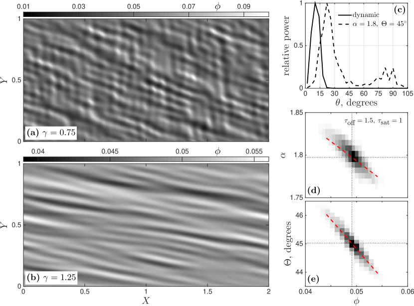
Figure 1: Comparison of numerical solutions to (1) and (2) with static and dynamic anisotropy. For both calculations, $r_{\beta}=1,\,R=1,\,r_{\xi}=5/3,\,\phi_{0}=0.05,\,\epsilon|\phi_{1}(\boldsymbol{X})|\leq 0.005$ and the domain is discretised into 600$\times$300 square cells. (a) Porosity field at a strain of 0.75 for a simulation with $\alpha=1.8$ and $\Theta=45^{\circ}$ throughout the domain. (b) Porosity field at a strain of 1.25 for a simulation with anisotropy calculated according to (3) and (4) with $\tau_{\textrm{sat}}=1,\,\tau_{\textrm{offset}}=1.5$. (c) Spectral power binned by wavefront-angle $\theta$ to the shear plane (after Katz et al., 2006) for the porosity fields shown in panels (a) and (b). Each spectrum is normalised by its maximum power. (d) and (e) Two-dimensional histograms derived from the simulation with dynamic anisotropy at a strain of 1.25 (after Katz and Takei, 2013, Fig. 12). Red dashed lines have a slope given by the ratio of perturbation quantities $\alpha_{1}/\phi_{1}$ and $\Theta_{1}/\phi_{1}$ from the stability analysis in §4.

Figure 1 compares solutions with fixed and dynamic anisotropy. In panel (a), anisotropy parameters are prescribed as $\alpha=\beta=1.8$, $\Theta=45^{\circ}$; in panel (b), these parameters are calculated cell-wise using equations (3) and (4), with $r_{\beta}=1$. Both calculations have $R=1$ (compaction length equal to domain height) and are initialised with the same porosity field, $\phi(\boldsymbol{X},t=0)=\phi_{0}+\epsilon\phi_{1}(\boldsymbol{X})$, where $\phi_{0}=0.05$ and $\epsilon=0.005$. $\phi_{1}(\boldsymbol{X})$ is a smooth, random field with unit amplitude, generated by filtering grid-scale white noise to remove variation at wavelengths below 15 grid-cells. Because the growth-rate of porosity perturbations differs for fixed and dynamic anisotropy, the simulations are shown at different values of the average simple-shear strain $\gamma$.

The different orientation of high-porosity features is evident in panels (a) and (b): dynamic anisotropy is associated with lower angles. This is quantified by the power spectrum in panel (c), where the power from a 2D fast-Fourier transform of the porosity field is binned according to the angle between the wavefront and the shear plane (Katz et al., 2006). Dynamic anisotropy produces a peak at $\sim 10^{\circ}$ whereas static anisotropy produces a peak at $\sim 23^{\circ}$. There is also a high-angle ($\sim 80^{\circ}$) peak for static anisotropy (corresponding to features visible in panel (a)) that does not survive at large strain. Panels (d) and (e) show the covariation of $\alpha$ and $\Theta$ with $\phi$ in panel (b); black dotted lines indicate mean values. These means are closely matched with the parameter values used in the fixed-anisotropy simulation. It is therefore clear that the difference in the dominant band angle (panel (c)) arises from the coupling between stress and the variations in $\alpha$ and $\Theta$. What is unclear, however, is the physical explanation for this difference and, indeed, why viscous anisotropy gives rise to bands at angles less than $45^{\circ}$ to the shear plane at all. We clarify these points below.

4 Linearised analysis with a perturbation-oriented coordinate system

Let $\epsilon\ll\phi_{0}$ be the initial amplitude of a porosity perturbation. We express the problem variables as a series expansion about the base-state in which the porosity is uniform and equal to $\phi_{0}$. We truncate the series after the first-order terms,

$$\left\{\begin{array}[]{ccccc}\phi(\boldsymbol{X},t)&=&\phi_{0}&+&\epsilon\phi_{1}(\boldsymbol{X},t)\\ P(\boldsymbol{X},t)&=&0&+&\epsilon P_{1}(\boldsymbol{X},t)\\ {\bf V}(\boldsymbol{X},t)&=&{\bf V}^{(0)}(\boldsymbol{X})&+&\epsilon{\bf V}^{(1)}(\boldsymbol{X},t)\\ \dot{e}_{ij}(\boldsymbol{X},t)&=&\dot{e}^{(0)}_{ij}&+&\epsilon\dot{e}^{(1)}_{ij}(\boldsymbol{X},t)\\ \tau_{ij}(\boldsymbol{X},t)&=&\tau^{(0)}_{ij}&+&\epsilon\tau^{(1)}_{ij}(\boldsymbol{X},t)\\ C_{ijkl}(\boldsymbol{X},t)&=&C^{(0)}_{ijkl}&+&\epsilon C^{(1)}_{ijkl}(\boldsymbol{X},t)\\ \alpha(\boldsymbol{X},t)&=&\alpha_{0}&+&\epsilon\alpha_{1}(\boldsymbol{X},t)\\ \Theta(\boldsymbol{X},t)&=&\Theta_{0}&+&\epsilon\Theta_{1}(\boldsymbol{X},t).\\ \end{array}\right.$$ (5)

The first term of (5) with index $0$ represents a simple-shear flow and its associated anisotropy, which is the base-state solution of order one ($\epsilon^{0}$), corresponding to the uniform porosity $\phi_{0}$. The second term of (5) with index 1 represents the perturbation of order $\epsilon^{1}$ caused by $\epsilon\phi_{1}$. By substituting (5) into equations (1), using $\mbox{\boldmath$\nabla$}\!\cdot{\bf V}^{(0)}=0$, and balancing terms at the order of $\epsilon^{1}$, we derive the governing equations for the perturbations as

$$\frac{\text{D}{\phi_{1}}}{\text{D}{t}} =(1-\phi_{0})\mbox{\boldmath$\nabla$}\!\cdot{\bf V}^{(1)}$$ (6a)

$$\mbox{\boldmath$\nabla$}\!\cdot{\bf V}^{(1)} =\displaystyle\frac{R^{2}}{r_{\xi}+4/3}\nabla^{2}P_{1}$$ (6b)

$$P_{1,i} =\left[C^{(1)}_{ijkl}\dot{e}^{(0)}_{kl}\right]_{,j}+\left[C^{(0)}_{ijkl}\dot{e}^{(1)}_{kl}\right]_{,j}\,\,(=\tau^{(1)}_{ij,j}),$$ (6c)

where $\text{D}\phi_{1}/\text{D}t=\partial\phi_{1}/\partial t+{\bf V}^{(0)}\cdot\mbox{\boldmath$\nabla$}\phi_{1}$.

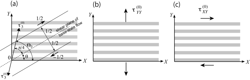
Figure 2: Schematic diagrams of the coordinate axes and porosity perturbation. (a) The coordinate system $(X,Y)$ for the linearised analysis is taken such that the $X$ axis is parallel to the initial perturbation wavefronts. The shear plane of the base-state, simple-shear flow is then rotated by an angle $\theta$. (b) The base-state normal stress $\tau^{(0)}_{YY}$ is oriented parallel to the initial perturbation wave vector. (c) The base-state shear stress $\tau^{(0)}_{XY}$ is parallel to the wavefronts.

Following previous studies, the porosity perturbations $\phi_{1}$ take the form of a plane wave oriented at a given angle to the base-state shear plane. Past workers chose to align the coordinate system with the base-state shear plane, such that the base-state strain rate tensor has a simple form (e.g. Spiegelman, 2003). Although the coordinate system was so aligned in the numerical models above, in this section the coordinates are rotated such that the $Y$ axis is parallel to the wave-vector of the initial perturbation, as shown in Figure 2. With this choice, $\theta$ again represents the angle between the perturbation wavefronts and the base-state shear plane. However, in the rotated coordinate system, $\Theta$ depends on both the direction of $\tau_{3}$ and the orientation of the bands. The base-state direction of maximum tensile stress $\tau_{3}$ makes an angle $\pi/4$ to the shear plane (eqn. (3)) and so for a coordinate rotation by $\theta$, we have $\Theta_{0}=\pi/4+\theta$ (Figure 2a).

In the following part of this section, we give an outline of the linearised approach, which shows that the new coordinate system reduces the complexity of the analysis and exposes the physical mechanisms of perturbation growth. This enables us to clarify the mechanics leading to low-angle bands in complicated problems such as under dynamic anisotropy. We first consider the base-state, simple shear flow at the order of $\epsilon^{0}$ (§4.1) and then the linearised governing equations at the order of $\epsilon^{1}$ (§4.2). Finally, in §4.3, we obtain the growth rate of porosity perturbations $\phi_{1}$ for the most general case of dynamic anisotropy. The result obtained is used in §5 to clarify the mechanisms of low-angle-band formation.

4.1 Base-state simple shear flow

Using the angle $\theta$ between the initial perturbation wavefronts (aligned with the $X$ direction) and the base-state shear plane (Fig. 2a), the components of the base-state strain rate tensor in the rotated coordinate system are

$$\dot{e}^{(0)}_{ij}=\frac{1}{2}\left(\begin{array}[]{cc}-\sin 2\theta&\cos 2\theta\\ \cos 2\theta&\sin 2\theta\end{array}\right).$$ (7)

As shown in Figs. 2b and 2c, $\tau^{(0)}_{YY}$ and $\tau^{(0)}_{XY}$ represent, respectively, the base-state tensile and shear stresses normal and parallel to the perturbation wavefronts, which play important roles in understanding the growth of these perturbations. Noting that $\dot{e}^{(0)}_{YY}=-\dot{e}^{(0)}_{XX}$, these components are given by

$$\left(\begin{array}[]{c}\tau^{(0)}_{YY}\\[2.84526pt] \tau^{(0)}_{XY}\end{array}\right)=\frac{1}{2}\left(\begin{array}[]{cc}C^{(0)}_{YYYY}-C^{(0)}_{YYXX}&2C^{(0)}_{YYXY}\\[2.84526pt] C^{(0)}_{XYYY}-C^{(0)}_{XYXX}&2C^{(0)}_{XYXY}\end{array}\right)\left(\begin{array}[]{c}\sin 2\theta\\[2.84526pt] \cos 2\theta\end{array}\right),$$ (8)

with $\Theta_{0}=\frac{\pi}{4}+\theta$. In Figure 3, $\tau^{(0)}_{YY}$ and $\tau^{(0)}_{XY}$ are plotted as a function of angle $\theta$. An understanding of their systematics is needed to interpret the results of the stability analysis.

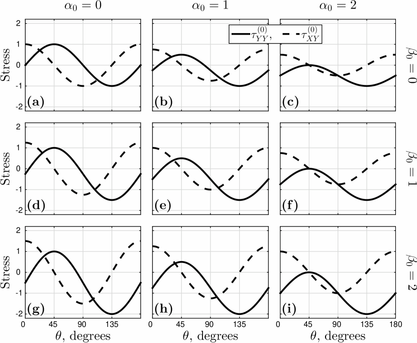
Figure 3: Normal stress $\tau^{(0)}_{YY}$ (tension positive) and shear stress $\tau^{(0)}_{XY}$ produced by the base-state simple shear flow as functions of angle $\theta$ between the shear plane and the $X$-axis (Fig. 2a). We use $r_{\xi}=5/3$ here and throughout (Takei and Katz, 2013). Each panel is computed with a different set $(\alpha_{0},\beta_{0})$ as labelled above and to the right of the panels.

Considering first the solid curves representing normal stress, we see that for $\alpha_{0}=\beta_{0}=0$ (isotropic, top-left panel), $\tau^{(0)}_{YY}$ follows the expected pattern of $\sin 2\theta$. It is tensile for $\theta<90^{\circ}$ and compressive for $\theta>90^{\circ}$ (Spiegelman, 2003). However, as $\alpha_{0}$ increases (for $\beta_{0}=0$, top row of panels), $\tau^{(0)}_{YY}$ becomes negative (compressive) at all angles. The mechanism for this change is two-fold. First, $\alpha_{0}$ decreases the viscous resistance to extension in the $\tau_{3}$ direction and reduces the maximum tensile stress. This is because increasing $\alpha_{0}$ reduces $(C^{(0)}_{YYYY}-C^{(0)}_{YYXX})$ for angles near $\theta=45^{\circ}$ (Figure 4a, black solid line). Superimposed on this is a compressive stress around $\theta=0^{\circ}$ and $90^{\circ}$ that emerges as a consequence of shear strain rate coupled to normal stress via the $C^{(0)}_{YYXY}$ viscosity (Figure 4a, gray solid line). The product $C^{(0)}_{YYXY}\dot{e}^{(0)}_{XY}$ is negative for all $\theta$, motivating us to name this coupling “shear-strain-induced compression.” This non-trivial result comes from the fact that the stress-induced softening occurs in the tensile ($\tau_{3}$) direction, as schematically illustrated in Takei and Katz (2013) Figure 7b.

The effect of increasing $\beta_{0}$ on $\tau^{(0)}_{YY}$ is shown down columns in Figure 3. Similar to $\alpha_{0}$, $\beta_{0}$ couples the shear strain rate to compressive normal stress for angles near $\theta=0^{\circ}$ and $90^{\circ}$ via the $C^{(0)}_{YYXY}$ viscosity. In contrast to $\alpha_{0}$, however, $\beta_{0}$ strengthens the aggregate in the $\tau_{1}$ direction and increases the normal stress amplitude near $\theta=135^{\circ}$ (Figures 3 and 4b). As a result, the sign-change of normal stress caused by $\beta_{0}$ occurs in a limited range of $\theta\lesssim 90^{\circ}$ and $\theta\gtrsim 0^{\circ}$ (Fig. 3, bottom-left panel).

The shear stress curves in Figure 3 (dashed lines) also change with increasing $\alpha_{0}$ and/or $\beta_{0}$. For zero anisotropy in panel (a), the shear stress follows $\cos 2\theta$, as expected for coordinate rotation only. Anisotropy does not change the mean of $\tau^{(0)}_{XY}(\theta)$, as required by symmetry of the stress tensor. Increasing $\alpha_{0}$ (or $\beta_{0}$) has an overall weakening (or strengthening) effect, changing only the amplitude of $\tau^{(0)}_{XY}$. This is in contrast to the effect of anisotropy on normal stress, which has a strong dependence on angle $\theta$.

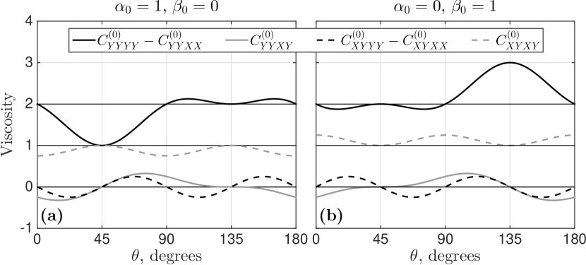
Figure 4: Viscosity components from equation (8) as functions of angle $\theta$ between the shear plane and the $X$-axis. The curves are computed for the anisotropy parameters (a) $\alpha_{0}=1$ and $\beta_{0}=0$, and (b) $\alpha_{0}=0$ and $\beta_{0}=1$. The thin black lines represent each component for the isotropic case ($\alpha_{0}=\beta_{0}=0$).

4.2 Growth of porosity perturbations

For simplicity in this linearised analysis, we consider the case of liquid viscosity $\eta_{L}=0$, giving a non-dimensional compaction length $R\rightarrow\infty$. In this limit, liquid segregation over any length scale occurs at vanishingly small pressure gradients. Therefore, the pressure gradient terms in equations (6c) are negligible. Pressure then drops out of the problem and we no longer need to solve equation (6b) (which has become indeterminate anyway!). This is equivalent to considering only the subset of perturbations with wavelengths much smaller than the dimensional compaction length (e.g. Katz et al., 2006).

Using the initial wavenumber vector $\boldsymbol{K}=(0,K)$, the porosity perturbation at time $t$ is

$$\phi_{1}(\boldsymbol{X},t)=\exp\left[i\boldsymbol{K}\cdot(\boldsymbol{X}-{\bf V}^{(0)}t)+\dot{s}t\right],$$ (9)

which accounts for rotation of the wave-vector due to advection by the base-state flow (Spiegelman, 2003). At $t=0$, by choice of the coordinate system, perturbations are uniform in the $X$ direction. Therefore, partial derivatives of the first-order quantities with respect to $X$ are zero. Using $\dot{e}^{(0)}_{XX}=-\dot{e}^{(0)}_{YY}$, $\dot{e}^{(1)}_{XX}=0$, and $\mbox{\boldmath$\nabla$}P_{1}=\boldsymbol{0}$, equations (6) become

$$\dot{s} =(1-\phi_{0})\dot{e}^{(1)}_{YY}/\phi_{1},$$ (10a)

$$0 =\left[(C^{(1)}_{YYYY}-C^{(1)}_{YYXX})\dot{e}^{(0)}_{YY}+2C^{(1)}_{YYXY}\dot{e}^{(0)}_{XY}\right]+\left[C^{(0)}_{YYYY}\dot{e}^{(1)}_{YY}+2C^{(0)}_{YYXY}\dot{e}^{(1)}_{XY}\right],$$ (10b)

$$0 =\left[(C^{(1)}_{XYYY}-C^{(1)}_{XYXX})\dot{e}^{(0)}_{YY}+2C^{(1)}_{XYXY}\dot{e}^{(0)}_{XY}\right]+\left[C^{(0)}_{XYYY}\dot{e}^{(1)}_{YY}+2C^{(0)}_{XYXY}\dot{e}^{(1)}_{XY}\right].$$ (10c)

Equations (10b) and (10c) are obtained after an integration in the $Y$ direction; boundary conditions are not needed because the domain is infinite and the first-order fields are periodic.

The right-hand side of equations (10b) and (10c) represent $\tau^{(1)}_{YY}$ and $\tau^{(1)}_{XY}$, respectively. Since pressure gradients are negligible, these stresses must be spatially uniform for the system to be in balance. Therefore the first-order product of viscosity and strain rate must sum to zero; viscosity reduction associated with porosity perturbations (within the first square brackets in the right hand side) is compensated by the strain rate perturbations (within the second square brackets).

To facilitate the physical interpretation of equations (10b) and (10c), these equations are re-expressed as

$$\left(\begin{array}[]{cc}C^{(0)}_{YYYY}&C^{(0)}_{YYXY}\\[2.84526pt] C^{(0)}_{XYYY}&C^{(0)}_{XYXY}\end{array}\right)\left(\begin{array}[]{c}\dot{e}^{(1)}_{YY}\\[2.84526pt] 2\dot{e}^{(1)}_{XY}\end{array}\right)=\left(\begin{array}[]{c}\tau^{(f)}_{YY}\\[2.84526pt] \tau^{(f)}_{XY}\end{array}\right),$$ (11)

with equivalent (“forcing”) stresses

$$\tau^{(f)}_{YY} =-\left[(C^{(1)}_{YYYY}-C^{(1)}_{YYXX})\dot{e}^{(0)}_{YY}+2C^{(1)}_{YYXY}\dot{e}^{(0)}_{XY}\right],$$ (12a)

$$\tau^{(f)}_{XY} =-\left[(C^{(1)}_{XYYY}-C^{(1)}_{XYXX})\dot{e}^{(0)}_{YY}+2C^{(1)}_{XYXY}\dot{e}^{(0)}_{XY}\right].$$ (12b)

Equation (11) relates the strain-rate response of the system to the forcing stresses defined by (12). From equation (11), normal strain rate in the $Y$ direction $\dot{e}^{(1)}_{YY}$ (the component that is most relevant to the perturbation growth) can be expressed as

$$\dot{e}^{(1)}_{YY}=\widetilde{C}^{(0)}_{YYYY}\tau^{(f)}_{YY}+\widetilde{C}^{(0)}_{YYXY}\tau^{(f)}_{XY},$$ (13)

where $\widetilde{C}^{(0)}_{YYYY}$ and $\widetilde{C}^{(0)}_{YYXY}$ are the compliances defined by

$$\widetilde{C}^{(0)}_{YYYY} =\frac{C^{(0)}_{XYXY}}{C^{(0)}_{XYXY}C^{(0)}_{YYYY}-C^{(0)}_{YYXY}C^{(0)}_{XYYY}},$$ (14a)

$$\widetilde{C}^{(0)}_{YYXY} =\frac{-C^{(0)}_{YYXY}}{C^{(0)}_{XYXY}C^{(0)}_{YYYY}-C^{(0)}_{YYXY}C^{(0)}_{XYYY}}.$$ (14b)

The forcing stresses, $\tau^{(f)}_{YY}$ and $\tau^{(f)}_{XY}$, are not externally applied (like those causing simple shear), nor are they the first-order stress perturbations $\tau^{(1)}_{YY}$ and $\tau^{(1)}_{XY}$ (these are both equal to zero). Instead, they are equivalent stresses that are created internally as a consequence of the base-state flow acting on the viscosity change associated with porosity perturbations. Moreover, under dynamic anisotropy, these forcing terms also depend on the strain-rate perturbations and hence equation (13) does not always give an explicit solution for $\dot{e}^{(1)}_{YY}$. Nonetheless, equation (13) enables us to separate the mechanics into two simpler parts: the forcing, $\tau^{(f)}_{YY}$ and $\tau^{(f)}_{XY}$, and the compliance, $\widetilde{C}^{(0)}_{YYYY}$ and $\widetilde{C}^{(0)}_{YYXY}$, where the latter represents the system response to forcing with unit amplitude. This decomposition is helpful to understand the detailed (and rather complicated) mechanisms of the different models considered here.

4.3 General solution

Equations (10) are solved here to obtain an explicit expression for $\dot{s}$ for the full model of dynamic anisotropy. The first-order viscosity tensor is written in terms of the porosity and anisotropy perturbations $\phi_{1}$, $\alpha_{1}$, $\beta_{1}$, and $\Theta_{1}$. The anisotropy perturbations are then expressed in terms of the porosity and strain-rate perturbations $\phi_{1}$, $\dot{e}^{(1)}_{YY}$, and $\dot{e}^{(1)}_{XY}$. These calculations are sketched in Appendix B. The components of the first-order viscosity tensor are then substituted into equations (10b) and (10c), which are manipulated to solve for $\dot{e}^{(1)}_{YY}$ and $\dot{e}^{(1)}_{XY}$ as functions of $\phi_{1}$. The normal strain rate $\dot{e}^{(1)}_{YY}$ obtained by this approach is substituted into (10a) to give an expression for the growth-rate of perturbations,

$$\dot{s}=(1-\phi_{0})\lambda\left[\widetilde{C}^{(0)}_{YYYY}\mathcal{D}_{p}\left(\tau_{YY}^{(0)}-q\tau_{XX}^{(0)}\right)+\widetilde{C}^{(0)}_{YYXY}\mathcal{D}_{q}\left(\tau_{XY}^{(0)}-p\tau_{XX}^{(0)}\right)\right],$$ (15)

with the compliances defined by (14) and dynamic factors

$$\mathcal{D}_{p} =\left(1-p{C^{(0)}_{XXXY}}/{C^{(0)}_{XYXY}}\right)/{D},$$ (16a)

$$\mathcal{D}_{q} =\left(1-q{C^{(0)}_{XXXY}}/{C^{(0)}_{YYXY}}\right)/{D},$$ (16b)

where

$$D=1+q\left(\tfrac{C^{(0)}_{XXXY}C^{(0)}_{XYYY}-C^{(0)}_{XYXY}C^{(0)}_{XXYY}}{C^{(0)}_{XYXY}C^{(0)}_{YYYY}-C^{(0)}_{YYXY}C^{(0)}_{XYYY}}\right)+p\left(\tfrac{C^{(0)}_{YYXY}C^{(0)}_{XXYY}-C^{(0)}_{XXXY}C^{(0)}_{YYYY}}{C^{(0)}_{XYXY}C^{(0)}_{YYYY}-C^{(0)}_{YYXY}C^{(0)}_{XYYY}}\right).$$ (17)

The constant coefficients $p$ and $q$ that express the sensitivity of the growth rate to dynamic anisotropy perturbations are

$$p =\zeta\displaystyle\frac{1-r_{\beta}}{4}\left(2\cos 2\theta-\frac{\alpha_{0}\Delta\tau^{(0)}}{\breve{\alpha}(\tau_{XX}^{(0)}-\tau_{YY}^{(0)})^{2}}\sin 2\theta\sin 4\theta\right),$$ (18a)

$$q =\zeta\frac{1-r_{\beta}}{4}\left(2\sin 2\theta+\frac{\alpha_{0}\Delta\tau^{(0)}}{\breve{\alpha}(\tau_{XX}^{(0)}-\tau_{YY}^{(0)})^{2}}\cos 2\theta\sin 4\theta\right)+\zeta\frac{1+r_{\beta}}{2},$$ (18b)

where $\breve{\alpha}$ and $\zeta$ are defined by equations (34) and (36), respectively. We do not attempt to physically interpret the detailed form of $p$ and $q$. It is important to note, however, that for the static anisotropy model, $p$ and $q$ are zero, and $\mathcal{D}_{p}=\mathcal{D}_{q}=1$.

5 Physical interpretation in various limits

The growth rate in eqn. (15) is a general result for the full model presented in §2 above (with the sole assumption of $R\to\infty$). To build up a physical understanding of this equation, we return to the simpler case of static anisotropy, which includes the simplest case of the Newtonian, isotropic model. The static anisotropy model has previously been studied by Takei and Katz (2013) using linearised analysis. However, the mathematical complexity of their results precluded a detailed mechanical interpretation. A reconsideration using the perturbation-oriented coordinate system enables a physical understanding of the instability mechanism and the rheological control on the dominant band angle. These are needed to understand the more complicated, dynamic model. To facilitate this (in §5.1–5.2), we make the simplifying assumption that $\beta=0$ — that there is no contiguity increase in the $\tau_{1}$-direction. The effect of non-zero $\beta$ is discussed in section 5.3, where we show that its role is minor compared to that of $\alpha$, the contiguity decrease in the $\tau_{3}$-direction.

5.1 Static anisotropy

When $\alpha_{1}=\beta_{1}=\Theta_{1}=0$, the mechanical equilibrium conditions (10b) and (10c) are written as

$$C^{(0)}_{YYYY}\dot{e}^{(1)}_{YY}+2C^{(0)}_{YYXY}\dot{e}^{(1)}_{XY} =\lambda\phi_{1}\tau^{(0)}_{YY}$$ (19a)

$$C^{(0)}_{XYYY}\dot{e}^{(1)}_{YY}+2C^{(0)}_{XYXY}\dot{e}^{(1)}_{XY} =\lambda\phi_{1}\tau^{(0)}_{XY}.$$ (19b)

Comparison with equation (11) shows that the forcing stresses are given by $\tau^{(f)}_{YY}=\lambda\phi_{1}\tau^{(0)}_{YY}$ and $\tau^{(f)}_{XY}=\lambda\phi_{1}\tau^{(0)}_{XY}$. These forcing stresses are caused by the base-state tensile and shear stresses acting on the porosity perturbation by way of porosity weakening rheology ($\lambda>0$) as depicted in Figs. 2b,c. In this simple model, $\tau^{(f)}_{YY}$ and $\tau^{(f)}_{XY}$ are given in terms of the porosity perturbation $\phi_{1}$, and hence eqn. (13) provides an explicit solution for $\dot{e}^{(1)}_{YY}$.

It is evident from (10a) that the normal strain rate $\dot{e}^{(1)}_{YY}$ causes an increase in the amplitude of porosity perturbations; the shear strain rate $\dot{e}^{(1)}_{XY}$ does not cause the porosity to change. When the viscosity is anisotropic, both the normal and the shear stress drive $\dot{e}^{(1)}_{YY}$ and hence contribute to perturbation growth. This does not occur under isotropic viscosity.

5.1.1 Instability mechanism in the isotropic system

For an isotropic aggregate ($\alpha_{0}=\beta_{0}=0$), $C^{(0)}_{YYXY}=C^{(0)}_{XYYY}=0$ in equations (11) and (19), and the compliance $\widetilde{C}^{(0)}_{YYXY}$ that couples shear stress to normal strain rate is zero. In this case, $\dot{e}^{(1)}_{YY}$ is driven only by the base-state normal stress $\tau_{YY}^{(0)}$. The growth rate $\dot{s}$ is given by

$$\dot{s}=(1-\phi_{0})\lambda\frac{\tau_{YY}^{(0)}}{C_{YYYY}^{(0)}}\hskip 28.45274pt\mbox{isotropic model.}$$ (20)

Perturbations are unstable under tensile stress ($\tau_{YY}^{(0)}>0$) normal to the perturbation wavefronts, stable under compressive normal stress ($\tau_{YY}^{(0)}<0$), and unaffected by shear stress $\tau_{XY}^{(0)}$. We therefore term this the tensile-stress-induced instability, or tensile instability. When band angle $\theta$ relative to the simple shear flow is $45^{\circ}$, the tensile stress $\tau_{YY}^{(0)}$ attains its maximum (Figure 3a) and hence the growth rate $\dot{s}$ is also at a maximum, as shown in Figure 5a and by Spiegelman (2003). The occurrence of the tensile instability in a porosity-weakening, two-phase aggregate was first predicted by Stevenson (1989).

5.1.2 Two instability mechanisms in the anisotropic system

For an anisotropic aggregate ($\alpha_{0}>0$ and/or $\beta_{0}>0$), there is a coupling between shear and normal components via $C^{(0)}_{YYXY}=C^{(0)}_{XYYY}\neq 0$. In this case, $\dot{e}^{(1)}_{YY}$ is forced by both normal stress across perturbations and shear stress along perturbations. The growth rate is

$$\dot{s}=(1-\phi_{0})\lambda\left(\widetilde{C}^{(0)}_{YYYY}\tau_{YY}^{(0)}+\widetilde{C}^{(0)}_{YYXY}\tau_{XY}^{(0)}\right)\hskip 28.45274pt\mbox{static anisotropy model,}$$ (21)

using the compliances given by equations (14). The first term on the right-hand side of (21) represents the tensile instability, generalised to the anisotropic aggregate. The 2nd term represents a shear-stress-induced instability that does not occur in the isotropic system. The total growth rate $\dot{s}$ versus band angle $\theta$ is plotted in the top row of panels of Figure 5 for various anisotropy amplitudes $\alpha_{0}$ (thick lines). Consistent with previous work, as $\alpha_{0}$ is increased, the single growth rate peak splits into two peaks at low and high angles to the shear plane (Fig. 5c). Because the lower-angle peak dominates the higher angle peak after a finite time (Katz et al., 2006; Takei and Katz, 2013), this result means a significant lowering of the dominant band angle by the viscous anisotropy — if the magnitude of anisotropy $\alpha$ is sufficiently close to saturation ($\alpha\simeq 2$).

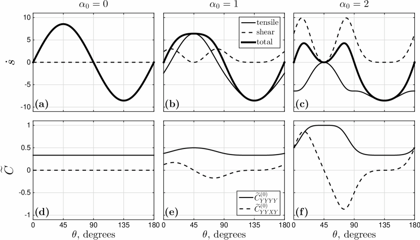
Figure 5: Characteristics of the static anisotropy model as a function of the angle between porosity perturbations and the shear plane. Each column is for a different value of $\alpha_{0}$. In all cases, $\beta_{0}=0$, $\lambda=27$, and $\phi_{0}=0.05$. Top row. Growth rate $\dot{s}$ of perturbations $\phi_{1}$ from eqn. (21). The heavy line represents the total growth rate; light lines show the growth rate decomposed into two parts: the contribution from the tensile instability (1st term of eqn. (21)) and that from the shear instability (2nd term). Bottom row. Compliances $\widetilde{C}^{(0)}_{YYYY}$ and $\widetilde{C}^{(0)}_{YYXY}$ in eqn. (21).

5.1.3 How viscous anisotropy causes lowering of band angle

Although the effect of viscous anisotropy is evident from the total growth rate shown in the top panels of Figure 5, it is not immediately obvious why the dominant band angle is lowered by viscous anisotropy. The physical mechanism can be understood by considering the tensile and shear components of the growth rate independently (1st and 2nd terms of (21), respectively). In the top row of Figure 5, these two growth rates are plotted separately for various values of $\alpha_{0}$ (thin solid curve for tensile instability; thin dashed curve for shear instability). Comparison of panels (a), (b), and (c) reveals that the peak split occurs through (i) stabilisation of the tensile instability and (ii) emergence of the shear instability with increasing magnitude of anisotropy $\alpha$. We consider each of these in turn.

To understand why viscous anisotropy stabilises the tensile instability, we return to the systematics of the base-state stress (section 4.1). Comparison of the three columns of Fig. 3 shows that as $\alpha_{0}$ increases, the tensile stress $\tau^{(0)}_{YY}$ decreases in amplitude and becomes compressive at all angles. With $\tau^{(0)}_{YY}\leq 0$, the first term in equation (21) is always less than or equal to zero, and hence stable.

To understand why viscous anisotropy destabilises the shear mechanism, we consider the coupling between the shear stress that drives the instability and the normal strain-rate that is responsible for its growth. As shown by equation (13) with $\tau^{(f)}_{YY}=\lambda\phi_{1}\tau^{(0)}_{YY}$ and $\tau^{(f)}_{XY}=\lambda\phi_{1}\tau^{(0)}_{XY}$, the shear stress $\tau^{(0)}_{XY}$ is coupled to the normal strain rate $\dot{e}^{(1)}_{YY}$ via $\widetilde{C}^{(0)}_{YYXY}$. The angular dependence of $\widetilde{C}^{(0)}_{YYXY}$ is shown by dashed curves in the bottom-row panels of Figure 5. If $\widetilde{C}^{(0)}_{YYXY}\tau^{(0)}_{XY}$ is positive, then $\dot{s}$ is positive (or $\dot{e}^{(1)}_{YY}$ is in phase with $\phi_{1}$) and the shear mechanism contributes to unstable growth of porosity perturbations. In fact, this product is positive (or zero) for all $\theta$, enabling us to name this coupling “shear stress-induced expansion.” This non-trivial result comes from the assumed microstructural behaviour: that stress-induced softening occurs in the tensile ($\tau_{3}$) direction, as illustrated in Takei and Katz (2013) Figure 7a. So the porosity perturbation grows because of the shear mechanism, for which the low angle is favorable.

5.1.4 Summary of static anisotropy model

As a recap and summary, note that under isotropic viscosity, the growth of bands at $45^{\circ}$ to the shear plane is caused by a tensile instability (Stevenson, 1989; Spiegelman, 2003). In contrast, under anisotropic viscosity, the peak growth rate of bands is controlled by a distinct shear instability. Although the peak growth rate of the shear instability occurs at $\theta<15^{\circ}$, stabilisation at these low angles by the tensile mechanism acts to give a maximum in the combined growth rate at $\theta=15^{\circ}$.

The comparison between isotropic and anisotropic systems developed above is summarised in the first two rows of Table 1. The tensile instability is separated into porosity-weakening $\lambda$, which is fundamental to all models, and the tensile stress across bands $\tau_{YY}^{(0)}$, which affects both isotropic and anisotropic cases. A shift of $\tau_{YY}^{(0)}$ to more negative, compressive values (represented by $\bigtriangleup$) stabilises the tensile instability. In contrast, the difference in shear instability can be simply shown by its existence or non-existence ($\bigcirc$ or –). It is the leading-order terms $\tau_{YY}^{(0)}$ and $\widetilde{C}^{(0)}_{YYXY}$ that are responsible for these differences.

Katz et al. (2006) extended the analysis of isotropic viscosity to include a power-law dependence of viscosity on strain rate (or, equivalently, on stress). They showed that strain-rate weakening viscosity leads to lowering of band angle. In the discussion section, we compare the angle-lowering mechanism of viscous anisotropy to that of the power-law viscosity. This is enabled by a reanalysis of the power-law model using the rotated coordinate system.

Table 1: Summary of band formation models. $\bigcirc$: exists; –: does not exist; $\bigtriangleup$: is modified.

	$\widetilde{C}^{(0)}_{YYYY}\,\tau^{(f)}_{YY}$ (tensile)			$\widetilde{C}^{(0)}_{YYXY}\,\tau^{(f)}_{XY}$ (shear)
Model	$\lambda>0$	$\tau^{(0)}_{YY}>0$	additional factor		Dominant angle
Isotropic Newtonian	$\bigcirc$	$\bigcirc$	–	–	$45^{\circ}$
Static anisotropy	$\bigcirc$	$\bigtriangleup$	–	$\bigcirc$	$\sim 23^{\circ}$
Dynamic anisotropy	$\bigcirc$	$\bigtriangleup$	$\bigcirc$	$\bigcirc$	$\sim 10^{\circ}$
Isotropic power-law	$\bigcirc$	$\bigcirc$	$\bigcirc$	–	$\sim 20^{\circ}$

5.2 Dynamic anisotropy

We return to the full expression for the growth rate of bands, eqn. (15), to develop a physical understanding of why dynamic anisotropy lowers band angles, as observed in the numerical solutions (Fig. 1). To do so we take $\alpha_{0}=1$ and again make the simplifying assumption that $\beta=0$ (though see §5.3, below).

The perturbations in $\Theta$ and $\alpha$ under dynamic anisotropy are obtained by linearisation of equations (3) and (4) with respect to the stress perturbation $\tau_{ij}^{(1)}$. The expansion is conducted around the base-state values $\Theta_{0},\alpha_{0}$. In Appendix B, we show that the sensitivity of $\alpha$ to variations in deviatoric stress is given by the parameter

$$\breve{\alpha}=\left.\frac{\partial{\alpha}}{\partial{\Delta\tau}}\right|_{\Delta\tau^{(0)}}=\frac{2}{\tau_{\textrm{sat}}}\text{sech}^{2}\left(\frac{2(\Delta\tau^{(0)}-\tau_{\textrm{offset}})}{\tau_{\textrm{sat}}}\right).$$ (22)

This parameter allows us to write $\alpha_{1}=\breve{\alpha}\Delta\tau^{(1)}$, and hence to see that static anisotropy corresponds to the case where $\breve{\alpha}=0$. The situation for $\Theta$ is more complicated because there is no single parameter that controls its sensitivity to deviatoric stress; variations of $\Theta$ can either be fully considered or fully neglected. Fortunately, numerical and analytical results show that these variations ($\Theta_{1}$) play an insignificant role in the understanding of band angles, and hence we need consider only the magnitude of anisotropy $\alpha$. This is achieved by looking at the dependence of key quantities (especially $\dot{s}$) on $\breve{\alpha}$.

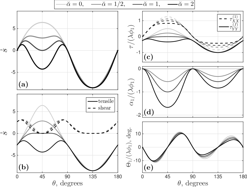
Figure 6: Characteristics of the dynamic anisotropy model for various values of $\breve{\alpha}$ as a function of the angle $\theta$ between porosity perturbations and the shear plane. In all panels, $\alpha_{0}=1$, $\beta_{0}=0$, $\lambda=27$, and $\phi_{0}=0.05$. (a) Full growth-rate $\dot{s}$ from eqn. (15). (b) Growth-rate from eqn. (15) split into the tensile-instability term (solid lines) and the shear-instability term (dashed lines). (c) Band-normal forcing stress (solid lines; eqn. (12a)) and band-parallel perturbation stress (dashed lines; eqn. (32)). Both are divided by $\lambda\phi_{1}$. Calculation details are in Appendix B. (d) and (e) The anisotropy perturbations $\alpha_{1}$ and $\Theta_{1}$ divided by $\lambda\phi_{1}$, calculated according to eqn. (35).

The growth-rate of porosity perturbations $\dot{s}$ is shown in panel (a) of Figure 6 for $\alpha_{0}=1$ and for values of $\breve{\alpha}$ ranging from zero to two. Although $\breve{\alpha}=0$ does not exclude linearised variations in $\Theta$, comparison with the $\dot{s}$-curve in Fig. 5b confirms that variations in $\Theta$ are ineffectual; with $\breve{\alpha}=0$ the expected band angle is $45^{\circ}$. For increasing $\breve{\alpha}$, the growth-rate peak again splits into peaks at low and high angles. It is important to note that the mean value of $\alpha$ ($\alpha_{0}$) is not changed in this exercise — only the amplitude of variations about that mean. Consistent with the numerical results of Figure 1, dynamic variations in the magnitude of anisotropy can sharply reduce band angles, even at moderate $\alpha_{0}$ for which the static anisotropy model predicts a high band angle ($45^{\circ}$).

Figure 6b breaks the full growth rate into two parts, each associated with one of the terms of equation (15). Dashed lines, representing the shear instability, are almost unaffected by $\breve{\alpha}$. In contrast, the tensile instability is strongly stabilised with increasing $\breve{\alpha}$. This stabilisation causes the peak of the full growth rate in panel (a) to split into low- and high-angle peaks. To understand why dynamic anisotropy promotes low band angles, it is therefore sufficient to understand why it stabilises the tensile instability.

The tensile instability is driven by $\tau^{(f)}_{YY}$, as discussed in §5.1. This represents the normal stress (tension positive) that arises when viscosity perturbations interact with the base-state strain rate. The detailed form of the forcing stress for the dynamic anisotropy model is given in equation (31). Figure 6c shows that the forcing normal stress $\tau^{(f)}_{YY}$ varies significantly with $\breve{\alpha}$ (whereas the forcing shear stress, not shown, is almost unaffected by $\breve{\alpha}$). The system compliances, which are leading-order quantities, are not affected by dynamic anisotropy. Therefore, it is the variation of $\tau^{(f)}_{YY}$ that is responsible for stabilisation of the tensile instability under dynamic anisotropy.

To develop a physical understanding of the detailed dependence of $\tau^{(f)}_{YY}$ on $\phi_{1}$, $\alpha_{1}$ and $\Theta_{1}$ (eqn. (31a)), focus attention on $\theta=45^{\circ}$, as this is the dominant band angle when $\breve{\alpha}=0$. For bands at $45^{\circ}$, solid curves in panel (c) of Figure 6 show that the forcing stress goes from a positive perturbation (in phase with $\phi_{1}$) to a negative perturbation (anti-phased with $\phi_{1}$) with increasing $\breve{\alpha}$ — hence the forcing stress $\tau_{YY}^{(f)}$ in the high-porosity bands goes from tensile to compressive. This change is due to an increase in the magnitude of anisotropy perturbation $\alpha_{1}=\breve{\alpha}\Delta\tau^{(1)}$, shown in panel (d). Since $\tau^{(1)}_{XY}=\tau^{(1)}_{YY}=0$, the deviatoric stress perturbation $\Delta\tau^{(1)}$ is entirely due to the band-parallel normal stress perturbation $\tau^{(1)}_{XX}$ (according to eqn. (32)), which is shown by dashed curves in panel (c). Because $\tau^{(0)}_{XX}<0$, $\tau^{(1)}_{XX}>0$ signifies a magnitude reduction of $\tau_{XX}$ in the high-porosity bands; the largest change occurs for bands at $\theta=45^{\circ}$. As sensitivity $\breve{\alpha}$ to deviatoric stress increases, $\alpha_{1}$ becomes more negative (panel (d)). Negative values of $\alpha_{1}$ (anti-phased with $\phi_{1}$) mean high-porosity bands have lower deviatoric stress and weaker anisotropy than the low-porosity, inter-band regions. This is consistent with numerical results in Fig. 1d.

Figure 5d–f shows that $\alpha_{0}$ increases the normal compliance $\widetilde{C}^{(0)}_{YYYY}$ at angles between zero and 90^∘. A negative perturbation to $\alpha_{0}$ therefore makes the high-porosity bands in this range of angles less compliant to tensile stress and the low-porosity inter-bands more compliant. Overall, then, the perturbation in anisotropy amplitude $\alpha_{1}$ tends to cancel the direct effect of the porosity perturbation $\phi_{1}$ on the normal compliance, and hence $\alpha_{1}$ works to stabilise the tensile instability.

The comparison between the static and dynamic anisotropy models developed in this section is summarised in Table 1. These two models are identical at leading order but different at first order. Therefore, stabilisation of the tensile mechanism due to more compressive base-state stress ($\tau_{YY}^{(0)}$) and destabilisation of the shear mechanism due to shear stress-induced expansion ($\widetilde{C}^{(0)}_{YYXY}$) occur in both the static and the dynamic anisotropy model. These two cases differ, however, in that further stabilisation of the tensile mechanism occurs due to the dynamic variation of anisotropy magnitude ($\alpha_{1}$). This effect hardens the band regions and weakens the inter-band regions under dynamic anisotropy. This additional factor ($\bigcirc$ in Table 1) significantly lowers the band angle.

It is interesting to note that dynamic perturbations to the angle of anisotropy $\Theta_{1}$ are not an important control on band angle. Figure 6e shows that they are not affected by $\breve{\alpha}$. More importantly, $\Theta_{1}$ is always zero for bands orientated at $\theta=45^{\circ}$. This indicates that the stabilisation of the tensile instability and the lowering of band angle under dynamic anisotropy cannot be attributed to $\Theta_{1}$. In numerical simulations (Fig. 1e), the variations of $\Theta$ do not contribute to the lowering of band angle that is observed in Fig 1c, though they are well-explained by the stability analysis at $\theta\simeq 10^{\circ}$ (red dashed line).

5.3 The effect of contiguity increase in the $\tau_{1}$-direction

Until now, we have neglected $\beta$ and focused on the effects of $\alpha$, which quantifies contiguity decrease in the direction of maximum tension. Non-zero $\alpha$ represents a weakening in the $\tau_{3}$ direction that (i) reduces the magnitude of tensile stress and leads to (ii) shear strain-induced compression and (iii) shear stress-induced extension (Takei and Katz, 2013). We have shown that the tensile mechanism is stabilised around $\theta=45^{\circ}$ by the first of these and is stabilised around $\theta=0^{\circ}$ and $90^{\circ}$ by the second; we have also shown that the shear mechanism is destabilised by (iii). The parameter $\beta$ quantifies the contiguity increase in the direction of maximum compression. Even if $\alpha$ is zero, a non-zero $\beta$ creates viscous anisotropy (see eqn. (2b)), causing the couplings (ii) and (iii). However, Fig. 4 shows that $\beta_{0}$ does not cause the weakening (i). It is this weakening, by $\alpha$ only, that is responsible for splitting the growth-rate peak in both static and dynamic models. On this basis, we expect the effect of $\beta_{0}$ to be small. This is indeed the case: as shown below, $\beta$ alone does not cause a lowering of band angle, but it can affect the lowering by $\alpha$.

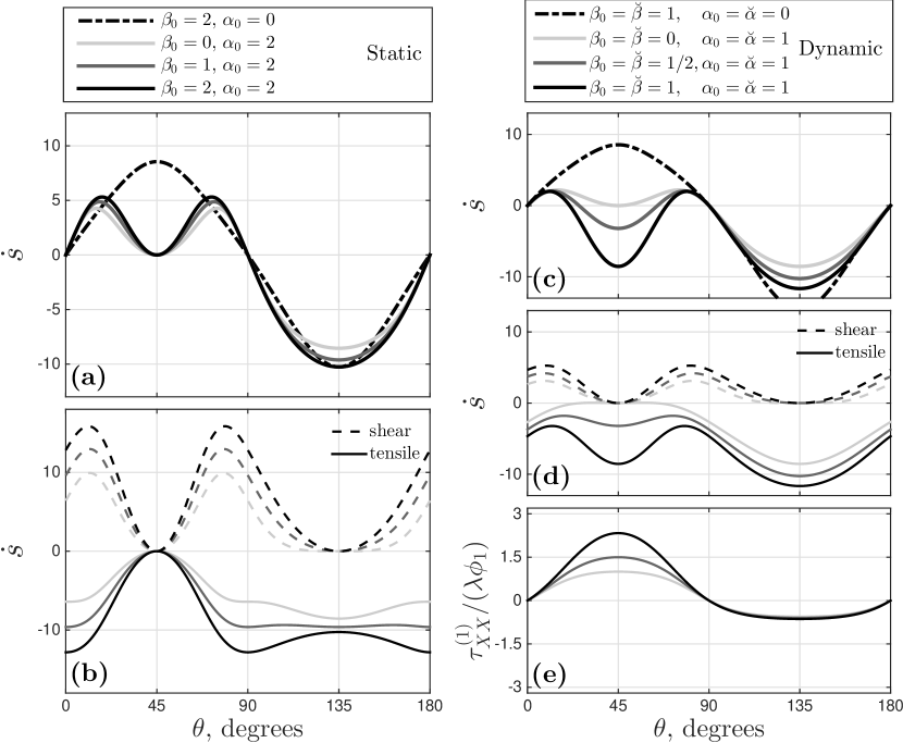
Figure 7: The effect of $\beta$ on the growth rate of porosity perturbations for static (left column) and dynamic (right column) anisotropy. (a) Full growth rate $\dot{s}$ from eqn. (21) for $\alpha_{0}=2$ and various values of $\beta_{0}$. A single curve for $\alpha_{0}=0$ and $\beta_{0}=2$ is also shown. In panel (b), the cases with $\alpha_{0}=2$ are decomposed into tensile and shear parts. Line greyscale has the same meaning as in panel (a); there is no curve for $\alpha_{0}=0$. (c) Full growth rate $\dot{s}$ from eqn. (15) for $\alpha_{0}=\breve{\alpha}=1$ and various values of $\beta_{0}=\breve{\beta}$. A single curve for $\alpha_{0}=\breve{\alpha}=0$ and $\beta_{0}=\breve{\beta}=1$ is also plotted. In panel (d), cases with $\alpha_{0}=\breve{\alpha}=1$ are decomposed into tensile and shear parts. (e) The band-parallel, normal stress perturbation $\tau^{(1)}_{XX}$.

The left column of Figure 7 illustrates the effect of $\beta$ under static anisotropy. Panel (a) shows that under static anisotropy, $\dot{s}$ is split into high and low angle peaks for any value of $\beta_{0}=0$ when $\alpha_{0}=2$ (solid curves), whereas it is peaked at $45^{\circ}$ for any value of $\beta_{0}$ when $\alpha_{0}=0$ ($\beta_{0}=2$ shown by dash-dot curve). For $\alpha_{0}=2$, increasing $\beta_{0}$ causes a modest shift to more compressive $\tau_{YY}^{(0)}$ at $\theta\sim 0^{\circ}$ and $\sim 90^{\circ}$ and a modest increase in the amplitude of shear stress $\tau_{XY}^{(0)}$ (Fig. 3, right column). Therefore, as Figure 7b shows, $\beta_{0}$ causes stabilisation of the tensile instability and destabilisation of shear instability in equal measure. These two effects compensate each other and the solid growth-rate curves in Figure 7a are thus all very similar to that for $\beta_{0}=0$.

The right column of Figure 7 shows how $\beta$ affects dynamic anisotropy. Panel (c) shows that for $\dot{s}$ in the dynamic anisotropy model, a two-peaked growth rate occurs for $\alpha_{0}=\breve{\alpha}=1$ and $\beta_{0}=\breve{\beta}=0$ (light gray curve) but does not for $\alpha_{0}=\breve{\alpha}=0$ and $\beta_{0}=\breve{\beta}=1$ (dash-dot curve). In the former case of non-zero $\alpha$ with a double peak, increasing $\beta_{0}$ enhances the stabilisation of the tensile mechanism at $45^{\circ}$ and deepens the valley between low-angle and high-angle peaks of $\dot{s}$ (Fig. 7c–d). This occurs because $\tau^{(1)}_{XX}$ is enhanced by the overall strengthening effect of $\beta_{0}$ (Fig. 7e). The very low band angles that emerge in the numerical simulation with dynamic anisotropy and $r_{\beta}=1$ (Fig. 1) are therefore a consequence of both the dynamic effect of $\alpha$ and the enhancement by $\beta$.

6 Summary and discussion

We have developed and analysed a model of coupled magma/mantle dynamics with anisotropic viscosity. The anisotropy is controlled by the orientation of principal stresses and the amount of deviatoric stress. The model presented here introduces small modifications on that of Takei and Katz (2013); in particular, the parameter $\beta$ models an increase in contiguity of grains in the direction of maximum compressive stress and the parameter $\tau_{\textrm{offset}}$ allows for a finer control on the magnitude of anisotropy and its sensitivity to stress (for $r_{\beta}=\textrm{const.}$). This description of viscous anisotropy is physically consistent with experiments and relatively simple, so its analysis should clarify the mechanics of rocks for which the assumptions hold. Existing experimental data, however, are not enough to quantitatively constrain all parameter values. The parameter studies performed here aim to understand the underlying physics.

It is known from previous theoretical work that anisotropic viscosity lowers the angle of emergent, high-porosity bands. Numerical solutions (Fig. 1) compare uniform anisotropy imposed a priori with anisotropy that varies according to local conditions of stress. They show that dynamic anisotropy leads to lowering of band angle as compared with uniform anisotropy, where the mean magnitude and angle from the dynamic case are used in the static case. Moreover, dynamic anisotropy produces low-angle bands even when its mean values wouldn’t do so if applied uniformly and held constant. The physical reasons for this have not previously been clear. Indeed, the question of why anisotropic viscosity lowers band angle at all has not previously been addressed.

Static viscous anisotropy, in which viscous resistance to extension in the most tensile direction is decreased, predicts low-angles of high-porosity bands for two reasons: (a) it suppresses the mode of instability in which tension causes extension across high-porosity bands; (b) it creates a mode of instability in which shear stress causes extension across high-porosity bands. The tensile instability has a peak perturbation growth rate in the maximum tensile direction ($\theta=45^{\circ}$). When this instability is suppressed by static anisotropy, the peak growth rate shifts to the smaller angles that are favoured by the emergent shear instability. And although the growth of the lowest angle bands are enhanced by the shear instability, perturbations parallel to the shear plane ($\theta=0^{\circ}$) are stable because of the compressive stress created by the base-state flow. Therefore, a low but finite angle of high-porosity bands is predicted by this model. Allowing for an increase in contiguity and viscosity in the direction of maximum compression has counter-balancing effects that leave predicted band angles almost unchanged.

Dynamic viscous anisotropy, in which the anisotropy parameters are allowed to vary with the local orientation and magnitude of deviatoric stress, tends to further lower band angles. It does so because it suppresses the tensile instability around $\theta=45^{\circ}$ via the following dynamic effect. Lower deviatoric stress in viscously weak bands gives lower anisotropy there, which makes them less compliant to tensile stress across them. Enhanced anisotropy in the interleaved, lower-porosity regions makes those regions more compliant. This effect over-compensates the compliance variations directly due to porosity weakening; it favours melt segregation from the bands into the inter-bands. Allowing for an increase in contiguity and viscosity in the direction of maximum compressional stress increases the contrast in band-parallel compressional stress (and deviatoric stress) between bands and inter-bands. This enhances the contrast in anisotropy and further suppresses the tensile instability. Dynamic anisotropy makes almost no modification to the shear instability.

The additional effects of dynamic anisotropy and the anisotropic increase of contiguity are important because they make more robust the prediction of low band angles. Under static anisotropy, the mean magnitude of anisotropy must be quite high to produce low-angle bands; moderate levels are insufficient. In contrast, under dynamic anisotropy with contiguity-increase in the direction of maximum compression, moderate levels of mean anisotropy efficiently produce low-angle bands. This helps to support the hypothesis that low-angle bands in experiments are due to anisotropic viscosity because it expands the parameter space in which the theoretical predictions should hold.

These conclusions were reached by use of stability analysis in a coordinate system that is rotated with respect to the plane of simple shear; in particular, the coordinate system is aligned with the wavefronts of the harmonic perturbations. This rotation leads to simpler expressions for the growth rate of perturbations: the tensile and shear modes appear as distinct terms that are amenable to physical understanding. For this reason, our analysis represents a framework in which to test and understand the family of rheologies that potentially produce low-angle bands in shearing flows. This includes variants of isotropic and anisotropic viscosity, but also potentially of dilatational granular rheology, damage, or composite rheologies (e.g. Rudge and Bercovici, 2015).

An application of the rotated coordinate system to the isotropic power-law creep model with stress exponent $n$ (Katz et al., 2006) is presented in Appendix A. As with all other models considered here, porosity perturbations reduce viscosity in the bands, resulting in the enhancement of the normal and shear strain rates, $\dot{e}^{(1)}_{YY}$ and $\dot{e}^{(1)}_{XY}$. In this model, however, the enhanced strain rates further reduce the viscosity, which feeds back to further enhance the strain rates. The importance of this non-Newtonian feedback relative to the porosity-weakening feedback is roughly approximated by $n-1$. Both normal and shear strain rates contribute to the non-Newtonian feedback; the relative importance of the shear component increases with increasing $r_{\xi}$. Therefore, if $n$ and $r_{\xi}$ are sufficiently large, shear strain rate is the key weakening factor and the growth rate reaches a maximum at a substantially lowered angle. However, in contrast to anisotropic viscosity, strain-rate weakening viscosity does not give rise to the shear instability — it merely lowers the most favorable angle for the tensile instability (comparison in Tab. 1). Although the details differ, both models predict an important role for shear stress in the lowering mechanism; both predict a low but finite angle with localised shear strain in the higher-porosity bands.

The model of viscous anisotropy used here seems promising as an explanation for laboratory experiments on deformation of partially molten rocks. Although its detailed form must be considered tentative, we are not aware of another theory that reproduces the low-angle bands found in experiments (Holtzman et al., 2003) while respecting the measured stress-dependence of creep viscosity (King et al., 2010). Furthermore, radially inward migration of magma in experiments employing torsional deformation (King et al., 2011; Qi et al., 2015) may be direct evidence of base-state segregation, a feature that arises naturally from viscous anisotropy (Takei and Katz, 2013) but may be impossible to reconcile with isotropic viscosity. Although the present study focuses on the angle of bands, the growth rate of bands is also affected by static and dynamic anisotropy; the growth rate is lowered by static anisotropy and further lowered by dynamic anisotropy (Figs. 5 and 6). This can be also discerned in the different total strain and different ranges of porosity in Figs. 1a and 1b. Therefore, a quantitative comparison between the measured and predicted growth rate becomes important for further refining and testing the theory.

In the present theory, $\alpha$, $\beta$, and $\Theta$ are assumed to depend on stress, based on the experimental results by Daines and Kohlstedt (1997) and Takei (2010). Although this assumption is considered to be valid at small strain, possible evolution of these parameters with increasing strain has to be investigated to model the system at large strains. Indeed, for more than 200% strain under simple shear, Zimmerman et al. (1999) observed that the long axis of melt pockets is predominantly oriented at an angle of $20^{\circ}$ from $\tau_{1}$; this is difficult to explain by stress alone. It should be noted, however, that microstructural analysis in laboratory studies has been performed in terms of shape and orientation of melt pockets; an analysis in terms of observed contiguity is more appropriate for comparison with and incorporation into the model. Numerical simulation using dynamic anisotropy and an empirically justified evolution equation for contiguity will be important in future work.

Acknowledgements   The research leading to these results has received funding from the European Research Council (ERC) under the European Union’s Seventh Framework Programme (FP7/2007–2013)/ERC grant agreement 279925. R.F.K. visited the Earthquake Research Institute of the University of Tokyo with support from the International Research Promotion Office; he is grateful for support by the Leverhulme Trust. Numerical simulations were performed at the Advanced Research Computing facility of the University of Oxford. The authors are grateful for stimulating discussions with M. Spiegelman, D.L. Kohlstedt, and C. Qi, and for helpful and encouraging reviews by S. Butler and two anonymous referees.

Appendix A Power-law creep model by Katz et al. (2006)

The model of band-formation under power-law viscosity by Katz et al. (2006) is formulated by equations (1) and the viscous constitutive relations

$$C_{ijkl}=\eta(\phi,\dot{e}_{II})　\times\bordermatrix{ij\!\downarrow&kl\!\rightarrow XX&YY&XY\cr XX&r_{\xi}+\frac{4}{3}&r_{\xi}-\frac{2}{3}&0\cr YY&\cdot&r_{\xi}+\frac{4}{3}&0\cr XY&\cdot&\cdot&1},$$ (23)

where only 6 of the 16 components of the two-dimensional version are shown due to the symmetry of $C_{ijkl}$. The normalised shear viscosity $\eta(\phi,\dot{e}_{II})$ depends on porosity and the second invariant of the strain-rate tensor, $\dot{e}_{II}=\sqrt{\dot{e}_{ij}\dot{e}_{ij}/2}$, as

$$\eta(\phi,\dot{e}_{II})=\exp\left[-\lambda(\phi-\phi_{0})/n\right]\dot{e}_{II}^{\frac{1-n}{n}}$$ (24)

(Katz et al., 2006; Takei and Holtzman, 2009b). Equation (24) represents a power-law viscosity that, to represent deformation by dislocation creep, has an exponent $n\approx 3.5$ (e.g. Karato and Wu, 1993) ($n=1$ corresponds to Newtonian viscosity). Under dislocation creep, the strain rate is highly sensitive to the stress because dislocation velocity and density both increase with increasing stress. Hence the model of Katz et al. (2006) incorporates strain-rate weakening in addition to the porosity weakening.

Katz et al. (2006) demonstrated that strain-rate weakening viscosity works to lower the band angle. Although the mechanism of this lowering is briefly discussed in their paper, further analysis of their model using the perturbation-oriented coordinate system is helpful to understand their explanation and to compare it with the mechanism of viscous anisotropy. For consistency with the foregoing development, $\eta_{L}=0$ is assumed here. We can expand (24) into base-state and perturbation terms as

$$\eta=\eta_{0}\left\{1-\epsilon\left[\frac{\lambda\phi_{1}}{n}+2\frac{n-1}{n}\left(2\dot{e}^{(0)}_{XY}\dot{e}^{(1)}_{XY}+\dot{e}^{(0)}_{YY}\dot{e}^{(1)}_{YY}\right)\right]\right\},$$ (25)

where $\eta_{0}=\left(\dot{e}_{II}^{(0)}\right)^{\frac{1-n}{n}}=2^{\frac{n-1}{n}}$ and we have used $\dot{e}_{II}^{(0)}=1/2$ and $\dot{e}^{(1)}_{XX}=0$. Combining (23) and (25) with stress balance (10b) and (10c), we obtain

$$C^{(0)}_{YYYY}\dot{e}^{(1)}_{YY} =\left[\frac{\lambda}{n}\phi_{1}+2\frac{n-1}{n}\left(\dot{e}^{(0)}_{YY}\dot{e}^{(1)}_{YY}+2\dot{e}^{(0)}_{XY}\dot{e}^{(1)}_{XY}\right)\right]\tau^{(0)}_{YY},$$ (26a)

$$2C^{(0)}_{XYXY}\dot{e}^{(1)}_{XY} =\left[\frac{\lambda}{n}\phi_{1}+2\frac{n-1}{n}\left(\dot{e}^{(0)}_{YY}\dot{e}^{(1)}_{YY}+2\dot{e}^{(0)}_{XY}\dot{e}^{(1)}_{XY}\right)\right]\tau^{(0)}_{XY}.$$ (26b)

This formulation is not the most amenable to inversion for the strain-rate perturbations, but it allows for a clear comparison with equations (11) and (12). We have moved terms to the right-hand side that can be considered to comprise the forcing stresses $\tau^{(f)}_{YY}$ and $\tau^{(f)}_{XY}$. Two points are evident: First, the forcing stresses retain the term representing base-state stress operating on porosity perturbations. Second, there are new terms that cross-couple the equations (26).

The cross-coupling terms in (26) arise because normal $\dot{e}_{YY}$ and shear $\dot{e}_{XY}$ components both affect $\dot{e}_{II}$ and hence modify the viscosity (by way of an increase in dislocation density). Two feedback mechanisms are thus at work, causing growth of porosity perturbations. The first of these is a direct effect: when $\lambda>0$, high-porosity bands are weaker by virtue of their higher porosity. The second is indirect: porosity-weakened bands have a larger strain-rate that, when $n>1$, further weakens them through the non-linear viscosity. The relative importance of the 2nd mechanism to the 1st one increases with increasing $n-1$.

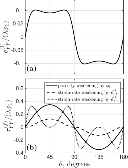
Figure 8: Characteristics of the power-law isotropic viscosity model as a function of the angle between porosity perturbations and the shear plane. In both panels, $n=5$. (a) Normal strain rate perturbation, which shows a double peak. (b) Forcing normal stress $\tau^{(f)}_{YY}$ due to porosity weakening (solid curve), strain-rate weakening associated with $\dot{e}^{(1)}_{YY}$ (dashed curve), and strain-rate weakening associated with $\dot{e}^{(1)}_{XY}$ (dotted curve). The three curves in panel (b) sum to the curve in panel (a).

Solving equations (26) for $\dot{e}^{(1)}_{YY}$ and $\dot{e}^{(1)}_{XY}$ and using equations (10a) and (23), the growth-rate is

$$\dot{s}=(1-\phi_{0})\frac{\lambda}{n}\frac{\tau_{YY}^{(0)}}{C^{(0)}_{YYYY}}\left[1-4\frac{n-1}{n}\left(\dot{e}^{(0)}_{XY}\right)^{2}-2\frac{n-1}{n}\left(1-\tfrac{r_{\xi}-2/3}{r_{\xi}+4/3}\right)\left(\dot{e}^{(0)}_{YY}\right)^{2}\right]^{-1}.$$ (27)

Takei and Holtzman (2009b) obtained the identical result for $\dot{s}$ and showed that a single peak splits into two at large $n$. Here, to understand the mechanism of the split, the forcing stress associated with tension, $\tau^{(f)}_{YY}$, is plotted in Figure 8b for each of the three terms in the RHS of (26a). Although the tensile forcing stress due to the porosity and normal-strain rate perturbations are maximum at $\theta=45^{\circ}$ (solid and dashed curves), that due to the enhanced shear strain rate $\dot{e}^{(1)}_{XY}$ has peaks at $\theta\simeq 10^{\circ}$ and $80^{\circ}$ (dotted curve). The sum of these three curves determines the profile of $\dot{e}^{(1)}_{YY}$ in panel (a) and hence determines the growth-rate. Panel (b) confirms that the weakening of viscosity by the enhanced shear-strain rate $\dot{e}^{(1)}_{XY}$ is the main cause of the peak split of the growth rate.

Appendix B Calculation of the dynamic-anisotropy growth rate

To solve the first-order equations of force balance (10), we need an expansion of the viscosity tensor into its base-state and perturbation components. Equation (2b) gives $C_{ijkl}$ as a function of $\phi$, $\alpha$, $\beta$, and $\Theta$. Under the dynamic anisotropy model, it is necessary to account for non-zero perturbations $\alpha_{1}$, $\beta_{1}$, and $\Theta_{1}$. In that case, $C^{(0)}_{ijkl}$ and $C^{(1)}_{ijkl}$ are calculated as

$$C^{(0)}_{ijkl} =C_{ijkl}(\phi_{0},\alpha_{0},\beta_{0},\Theta_{0}),$$ (28a)

$$C^{(1)}_{ijkl} =\displaystyle\left.\frac{\partial{C_{ijkl}}}{\partial{\phi}}\right|_{0}\,\phi_{1}+\left(\left.\frac{\partial{C_{ijkl}}}{\partial{\alpha}}\right|_{0}+r_{\beta}\left.\frac{\partial{C_{ijkl}}}{\partial{\beta}}\right|_{0}\right)\alpha_{1}+\left.\frac{\partial{C_{ijkl}}}{\partial{\Theta}}\right|_{0}\,\Theta_{1}.$$ (28b)

From the equation for anisotropy magnitude (4a),

$$\alpha_{0}=1+\tanh\left(\frac{2\Delta\tau^{(0)}-2\tau_{\textrm{offset}}}{\tau_{\textrm{sat}}}\right),$$ (29)

where $\Delta\tau^{(0)}=2(1-(\alpha_{0}-\beta_{0})/4)$. Then from equation (28b), the stress perturbation is written as

$$\tau^{(1)}_{ij}=C^{(0)}_{ijkl}\dot{e}^{(1)}_{kl}-\lambda\phi_{1}\tau_{ij}^{(0)}+\alpha_{1}\left(\left.\frac{\partial{C_{ijkl}}}{\partial{\alpha}}\right|_{0}+r_{\beta}\left.\frac{\partial{C_{ijkl}}}{\partial{\beta}}\right|_{0}\right)\dot{e}^{(0)}_{kl}+\Theta_{1}\left.\frac{\partial{C_{ijkl}}}{\partial{\Theta}}\right|_{0}\dot{e}^{(0)}_{kl}.$$ (30)

Using (30), (2b), (7), and $\Theta_{0}=\pi/4+\theta$, the mechanical equilibrium conditions $\tau^{(1)}_{XY}=\tau^{(1)}_{YY}=0$ from equations (10) are written as

$$C^{(0)}_{YYYY}\dot{e}^{(1)}_{YY}+2C^{(0)}_{YYXY}\dot{e}^{(1)}_{XY} =\lambda\phi_{1}\tau_{YY}^{(0)}+\frac{1-r_{\beta}}{4}\left(\alpha_{1}\sin 2\theta+2\alpha_{0}\Theta_{1}\cos 2\theta\right)+\frac{1+r_{\beta}}{4}\alpha_{1},$$ (31a)

$$C^{(0)}_{XYYY}\dot{e}^{(1)}_{YY}+2C^{(0)}_{XYXY}\dot{e}^{(1)}_{XY} =\lambda\phi_{1}\tau_{XY}^{(0)}+\frac{1-r_{\beta}}{4}\left(\alpha_{1}\cos 2\theta-2\alpha_{0}\Theta_{1}\sin 2\theta\right),$$ (31b)

where the right-hand sides of these equations are the dynamic-anisotropy version of the forcing stresses $\tau^{(f)}_{YY}$ and $\tau^{(f)}_{XY}$, respectively. The normal-stress perturbation in the $X$-direction is

$$\tau^{(1)}_{XX} =C^{(0)}_{XXYY}\dot{e}^{(1)}_{YY}+2C^{(0)}_{XXXY}\dot{e}^{(1)}_{XY}-\lambda\phi_{1}\tau_{XX}^{(0)}$$

$$-\frac{1+r_{\beta}}{4}\alpha_{1}+\frac{1-r_{\beta}}{4}\left(\alpha_{1}\sin 2\theta+2\alpha_{0}\Theta_{1}\cos 2\theta\right).$$ (32)

Microstructural anisotropy is determined by deviatoric stress. From the total differentials of equations (3) and (4a), and from $\tau_{XY}^{(1)}=\tau_{YY}^{(1)}=0$, $\alpha_{1}$ and $\Theta_{1}$ are related to $\tau_{XX}^{(1)}$ as

$$\alpha_{1} =\breve{\alpha}\Delta\tau^{(1)}=\breve{\alpha}\frac{\tau_{XX}^{(0)}-\tau_{YY}^{(0)}}{\Delta\tau^{(0)}}\tau_{XX}^{(1)},$$ (33a)

$$\Theta_{1} =-\frac{\sin 4\Theta_{0}}{4}\frac{\tau_{XX}^{(1)}}{\tau_{XX}^{(0)}-\tau_{YY}^{(0)}},$$ (33b)

with

$$\breve{\alpha}=\left.\frac{\partial\alpha}{\partial\Delta\tau}\right|_{\Delta\tau=\Delta\tau^{(0)}}=\frac{2}{\tau_{\textrm{sat}}}\mbox{sech}^{2}\displaystyle\left(\frac{2(\Delta\tau^{(0)}-\tau_{\textrm{offset}})}{\tau_{\textrm{sat}}}\right).$$ (34)

Then we use the expression (32) for $\tau_{XX}^{(1)}$ and equations (33) to obtain

$$\alpha_{1} =2\zeta\left(C^{(0)}_{XXYY}\dot{e}^{(1)}_{YY}+2C^{(0)}_{XXXY}\dot{e}^{(1)}_{XY}-\lambda\phi_{1}\tau_{XX}^{(0)}\right),$$ (35a)

$$\Theta_{1} =\frac{\zeta\Delta\tau^{(0)}\sin 4\theta}{2\breve{\alpha}(\tau_{XX}^{(0)}-\tau_{YY}^{(0)})^{2}}\left(C^{(0)}_{XXYY}\dot{e}^{(1)}_{YY}+2C^{(0)}_{XXXY}\dot{e}^{(1)}_{XY}-\lambda\phi_{1}\tau_{XX}^{(0)}\right),$$ (35b)

where

$$\zeta^{-1}=\left(\frac{1+r_{\beta}}{2}-\frac{1-r_{\beta}}{2}\sin 2\theta\right)+\frac{2\Delta\tau^{(0)}}{\breve{\alpha}(\tau_{XX}^{(0)}-\tau_{YY}^{(0)})}\left[1-\frac{(\alpha_{0}-\beta_{0})}{8(\tau_{XX}^{(0)}-\tau_{YY}^{(0)})}\cos 2\theta\sin 4\theta\right].$$ (36)

Equations (35) can be substituted into the stress-balance equations (31) giving a system in which the only first-order quantities are $\phi_{1}$, $\dot{e}^{(1)}_{XY}$, and $\dot{e}^{(1)}_{YY}$.

References

- Allwright and Katz [2014] J. Allwright and R. Katz. Pipe poiseuille flow of viscously anisotropic, partially molten rock. Geophys. J. Int., 199(3):1608–1624, 2014. doi: 10.1093/gji/ggu345.
- Balay et al. [2001] S. Balay, K. Buschelman, W. Gropp, D. Kaushik, M. Knepley, L. McInnes, B. Smith, and H. Zhang. http://www.mcs.anl.gov/petsc, 2001.
- Balay et al. [2004] S. Balay, K. Buschelman, W. Gropp, D. Kaushik, M. Knepley, L. McInnes, B. Smith, and H. Zhang. PETSc users manual. Technical report, Argonne National Lab, 2004.
- Butler [2012] S. Butler. Numerical Models of Shear-Induced Melt Band Formation with Anisotropic Matrix Viscosity. Phys. Earth Planet. In., 200-201:28–36, 2012. doi: 10.1016/j.pepi.2012.03.011.
- Cooper et al. [1989] R. Cooper, D. Kohlstedt, and K. Chyung. Solution-precipitation enhanced creep in solid–liquid aggregates which display a non-zero dihedral angle. Acta Metall, 37:1759–1771, 1989.
- Daines and Kohlstedt [1997] M. Daines and D. Kohlstedt. Influence of deformation on melt topology in peridotites. J. Geophys. Res., 102:10257–10271, 1997.
- Drew [1983] D. Drew. Mathematical modeling of two-phase flow. Annual Review Of Fluid Mechanics, 15:261–291, 1983. doi: 10.1146/annurev.fl.15.010183.001401.
- Holtzman and Kohlstedt [2007] B. Holtzman and D. Kohlstedt. Stress-driven melt segregation and strain partitioning in partially molten rocks: Effects of stress and strain. J. Petrol., 48:2379–2406, 2007. doi: 10.1093/petrology/egm065.
- Holtzman et al. [2003] B. Holtzman, N. Groebner, M. Zimmerman, S. Ginsberg, and D. Kohlstedt. Stress-driven melt segregation in partially molten rocks. Geochem. Geophys. Geosys., 4, 2003. doi: 10.1029/2001GC000258.
- Karato and Wu [1993] S. Karato and P. Wu. Rheology of the upper mantle - a synthesis. Science, 260, 1993.
- Katz and Takei [2013] R. Katz and Y. Takei. Consequences of viscous anisotropy in a deforming, two-phase aggregate: 2. Numerical solutions of the full equations. J. Fluid Mech., 734:456–485, 2013. doi: 10.1017/jfm.2013.483.
- Katz et al. [2006] R. Katz, M. Spiegelman, and B. Holtzman. The dynamics of melt and shear localization in partially molten aggregates. Nature, 442, 2006. doi: 10.1038/nature05039.
- Katz et al. [2007] R. Katz, M. Knepley, B. Smith, M. Spiegelman, and E. Coon. Numerical simulation of geodynamic processes with the Portable Extensible Toolkit for Scientific Computation. Phys. Earth Planet. In., 163:52–68, 2007. doi: 10.1016/j.pepi.2007.04.016.
- King et al. [2010] D. King, M. Zimmerman, and D. Kohlstedt. Stress-driven melt segregation in partially molten olivine-rich rocks deformed in torsion. J. Petrol., 51:21–42, 2010. doi: 10.1093/petrology/egp062.
- King et al. [2011] D. S. H. King, B. K. Holtzman, and D. L. Kohlstedt. An experimental investigation of the interactions between reaction-driven and stress-driven melt segregation: 1. Application to mantle melt extraction. Geochemistry Geophysics Geosystems, 12, 2011. doi: 10.1029/2011GC003684.
- McKenzie [1984] D. McKenzie. The generation and compaction of partially molten rock. J. Petrol., 25, 1984.
- Mei et al. [2002] S. Mei, W. Bai, T. Hiraga, and D. Kohlstedt. Influence of melt on the creep behavior of olivine-basalt aggregates under hydrous conditions. Earth Plan. Sci. Lett., 201:491–507, 2002.
- Qi et al. [2015] C. Qi, D. Kohlstedt, R. Katz, and Y. Takei. An experimental test of the viscous anisotropy hypothesis for partially molten rocks. Proc. Nat. Acad. Sci., 2015. doi: 10.1073/pnas.1513790112.
- Rudge and Bercovici [2015] J. Rudge and D. Bercovici. Melt-band instabilities with two-phase damage. Geophys. J. Int., 201(2):640–651, 2015. doi: 10.1093/gji/ggv040.
- Rudge et al. [2011] J. F. Rudge, D. Bercovici, and M. Spiegelman. Disequilibrium melting of a two phase multicomponent mantle. Geophys. J. Int., 184(2):699–718, 2011.
- Simpson et al. [2010a] G. Simpson, M. Spiegelman, and M. Weinstein. A multiscale model of partial melts: 1. Effective equations. Journal Of Geophysical Research, 115, 2010a. doi: 10.1029/2009JB006375.
- Simpson et al. [2010b] G. Simpson, M. Spiegelman, and M. Weinstein. A multiscale model of partial melts: 2. Numerical results. Journal Of Geophysical Research, 115, 2010b. doi: 10.1029/2009JB006376.
- Spiegelman [2003] M. Spiegelman. Linear analysis of melt band formation by simple shear. Geochem. Geophys. Geosys., 2003. doi: 10.1029/2002GC000499.
- Stevenson [1989] D. Stevenson. Spontaneous small-scale melt segregation in partial melts undergoing deformation. Geophys. Res. Letts., 16, 1989.
- Takei [1998] Y. Takei. Constitutive mechanical relations of solid-liquid composites in terms of grain-boundary contiguity. Journal Of Geophysical Research, 103:18183–18203, 1998.
- Takei [2010] Y. Takei. Stress-induced anisotropy of partially molten rock analogue deformed under quasi-static loading test. Journal Of Geophysical Research, 115:B03204, 2010. doi: 10.1029/2009JB006568.