Abstract

Chimera is a relatively new emerging phenomenon where coexistence of synchronous and asynchronous state is observed in symmetrically coupled dynamical units. We report observation of the chimera state in multiplex networks where individual layer is represented by 1-d lattice with non-local interactions. While, multiplexing does not change the type of the chimera state and retains the multi-chimera state displayed by the isolated networks, it changes the regions of the incoherence. We investigate emergence of coherent-incoherent bifurcation upon varying the control parameters, namely, the coupling strength and the network size. Additionally, we investigate the effect of initial condition on the dynamics of the chimera state. Using a measure based on the differences between the neighboring nodes which distinguishes smooth and non-smooth spatial profile, we find the critical coupling strength for the transition to the chimera state. Observing chimera in a multiplex network with one to one inter layer coupling is important to gain insight to many real world complex systems which inherently posses multilayer architecture.

1 Introduction

In past few decades, network science has discovered a plethora of novel phenomena while trying to mimic real world systems in a better manner. One of such discovery is an observation of the chimera state. It was first reported by Kuramato et. al. in 2002 while investigating non locally coupled identical oscillators in a ring network  [Kuramoto & Battogtokh (2002)]. Later, it was analyzed and christened by Abrams and Strogatz in 2006 as chimera state  [Abrams & Strogatz (2006)]. Like, its counterpart in Greek mythology, a chimera state has come to be referred as a mathematical hybrid state in which coherent and incoherent dynamics coexist in non-locally coupled identical oscillators in a structurally symmetric network.

Chimera has been extensively investigated both theoretically [Sethia et al. (2008), Laing (2009), Omelchenko et al. (2011)] and experimentally [Hagerstrom et al. (2012), Larger et al. (2013)]. It has been observed in plenty of networks including phase oscillators [Abrams et al. (2004)), Abrams & Strogatz (2006), Maistrenko et al. (2014), Omel’chenko et al. (2012), Sethia et al. (2008), Laing (2009)], chemical [Tinsley et al. (2012), Nkomo et al. (2013)], mechanical oscillators [Martens et al. (2013)], neuron models [Hizanidis et al. (2014)], planar oscillators [Laing (2010)], boolean networks [Rosin et al. (2014), Rosin (2015)], 1D superconducting meta material [Lazarides et al. (2015)], etc. Chimera was originally reported for non-locally coupled oscillators, recently it has been reported in feed back delayed networks [Omel’chenko et al. (2008), Sheeba et al. (2010)], globally coupled networks [Schmidt et al. (2014), Yeldesbay et al. (2014)], time varying networks [Buscarino et al. (2015)] and networks with purely local coupling [Laing (2015)]. Moreover, different types of chimera has been reported including multi cluster chimera [Xie et al. (2014), Omelchenko et al. (2013)], virtual [Larger et al. (2013)], breathing [Abrams et al. (2008)] and two dimensional chimera [Omel’chenko et al. (2012), Panaggio & Abrams (2015)]. A recent work suggests emergence of Chimera, dependent on nonhyperbolicity of dynamical systems for both the time-discrete and time continuous cases [Semenova et al. (2015)].

The chimera state has also been reported for various real world networks models such as Rosenzweig-MacArthur oscillators for ecological networks [Dutta & Banerjee (2015)]. Chimera has also been characterized by the state of the dynamical evolution of the network. Type - I chimera is characteristic of the hyper chaotic behavior with many positive Lyapunov exponents [Wolfrum et al. (2011)]. This type of chimera has primarily been observed for time-continuous systems like complex Ginzburg-Landau oscillators or Kuramoto oscillators. In Type-II chimera, only spatial chaos has been observed with a rather simple temporal behavior (mostly periodic). Though, this type of chimera has been reported mainly for the time-discrete systems (maps) [Omelchenko et al. (2011), Omelchenko et al. (2012), Hagerstrom et al. (2012)], it has recently been observed for the time-continuous Stuart-Landau oscillators as well [Zakharova et al. (2014)].

Further, modeling real world complex systems under the multiplex network framework is one of the recent advancements in the network theory [Boccaletti et al. (2014), Lee et al. (2012), Wang et al. (2015), Kivelä et al. (2014)]. We consider a multiplex network consisting of the same nodes across the layers (Fig. 1) and investigate the occurrence of chimera state in the multiplex ring networks. In this structure, each node has exactly the same connection architecture. We observe Type-II chimera with spatial chaos and periodic temporal behavior. Though, the chimera state, upon multiplexing, remains of the same type as observed for the isolated network, the multiplexing changes the region of incoherence. Dependence of the chimera state on initial conditions is observed for the multiplex networks as already observed for the isolated networks. Additionally we present a measure in terms of distance variable to distinguish between the coherent and the chimera state and to identify the transition point for the coherent-incoherent bifurcation. We also investigate role of the size of the network in determining the critical coupling strength for the symmetry breaking and thus emergence of the chimera state.

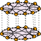
Figure 1: Schematic diagram for multiplex network consisting of two layers. Each layer is represented by 1D lattice with non-local interaction. Each node (circle) has the same coupling architecture.

2 Model

We consider a multiplex $S^{1}$ ring network with N nodes in each layer, where $S^{1}$ represents one dimensional symmetric cyclic group with elements being invariant to the permutation operation [Jacobson (2009)]. Considering $z_{t}(i),i=1,...,mN$ as a real dynamical variable at time $t$ for the $i^{th}$ node, the dynamics of the network can be described as,

$$z_{t+1}(i)=f(z_{t}(i))+\frac{\varepsilon}{(2rN+1)}\sum_{j=1}^{mN}A_{ij}[f(z_{t}(j))-f(z_{t}(i))]$$ (1)

where $\varepsilon$ represents the coupling strength, $m$ represent number of layers, $r$ represents the coupling radius defined by $r=P/N$, with $P$ signifying the number of neighbours in each direction in a layer. The elements of the adjacency matrix A of a network is defined as $A_{ij}=1$ or $0$ depending upon whether $i^{th}$ and $j^{th}$ nodes are connected or not. The diagonal entries $A_{ij}=0$ represents no self connection in the network. The adjacency matrix $A$ for the multiplex network can be written as,

$$A=\begin{pmatrix}A^{1}&I&.&.&.&I\\ I&A^{2}&I&.&.&I\\ .&I&A^{3}&.&.&.\\ .&.&.&.&.&.\\ .&.&.&.&.&.\\ I&.&.&.&.&A^{m}\\ \end{pmatrix},$$

where $A^{1}$,$A^{2}$,…,$A^{m}$ represent the adjacency matrix of the first, second,…,$m^{th}$ layer, respectively and $I$ is an unit NxN matrix. Note that the number of nodes in each layer of the multiplex network is same. A mismatch in the network size of the layers will yield nodes in different layers having different interaction patterns and hence we can not define the chimera state. We use logistic map $f(z)=\mu z(z-1)$ with the bifurcation parameter $\mu=3.8$ at which individual logistic map exhibits chaotic behavior. We consider coupling radius $r=0.32$ for each layer indicating degree of each node being 64. A state of the network is defined as spatially coherent if for any node $i\in S^{1}$, the spatial distance between the neighboring nodes approaches to zero for $t\rightarrow\infty$

$$\lim\limits_{t\rightarrow\infty}\mid{z_{t}(i+1)-z_{t}(i)}\mid\rightarrow 0,\,\,\,\,\forall\;i\in S^{1}$$ (2)

Geometrically, this signifies a smooth profile of the spatial curve. Smoothness of the curve, signifying the correlated spatial values of the neighboring nodes, is defined with the absence of any discontinuity in the spatial curve. Whereas, temporal coherence (synchronization) is defined as, $\lim\limits_{t\rightarrow\infty}\mid{z_{t}(j)-z_{t}(i)}\mid\rightarrow 0$ for $\forall\;i,j\in S^{1}$. Therefore, temporal coherence can be written as $z_{t}(1)=z_{t}(2)=......=z_{t}$ which leads to a straight line for the spatial curve associated with the temporal coherence.

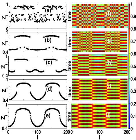
Figure 2: Snapshots and spatio-temporal plots for multiplex $S^{1}$ ring network. (a) and (f) are for $\varepsilon=0.1$, (b) and (g) $\varepsilon=0.28$, (c) and (h) $\varepsilon=0.30$, (d) and (i) $\varepsilon=0.40$, (e) and (j) $\varepsilon=0.44$. Number of nodes in each layer remains $N=100$ and coupling radius $r=0.32$. Initial transient is taken as 5000. results are presented for time range 5000 to 5015.

Appearance of discontinuity in the smooth spatial curve implies coexistence of the coherence and incoherence regions. To demonstrate the absence of smoothness, we define a measure based on the spatial distance as follows,

$$d(i)=(z(i+1)-z(i))-(z(i)-z(i-1))$$ (3)

which captures the difference of the spatial distances between the neighboring nodes. For smooth spatial profile $d(i)=0$, signifying a symmetric distribution of the distances between neighboring nodes, while discontinuity in the spatial profile, signifying the transition point, is indicated as kinks in the distribution. We use this measure to find the critical coupling strength for the symmetry breaking and thus resulting the chimera state.

3 Coherent-Incoherent bifurcation

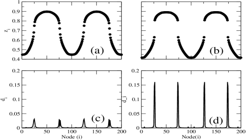
Figure 3: Distance measure for multiplex $S^{1}$ ring network (a),(c) for $\varepsilon=0.44$ and (b),(d) for $\varepsilon=0.4$. Network size is $N=100$ in each layer and coupling range is $r=0.32$.

We evolve Eq. 1 starting with a set of special initial conditions and after an initial transient, study the spatio temporal patterns of the multiplex network. Note that uniform or the Gaussian distributed random initial conditions lead to either a completely coherent, spanning all the nodes, or a completely incoherent state depending upon the coupling strength. For $0.28\leq\varepsilon\leq 0.32$ leads to the incoherent evolution of all the nodes. Motivated from [Kuramoto & Battogtokh (2002), Abrams & Strogatz (2006)], we use a hump back function to generate initial conditions as follows. We choose an uniform random number $z_{0}(i)$ for initial state for $i^{th}$ node within some interval which varies like a Gaussian function as:

$$z_{0}(i)=exp\big{[}-\frac{(i-\frac{N}{2})^{2}}{2\sigma^{2}}\big{]}$$ (4)

The variance $\sigma$ is chosen depending upon the size of the network such that the random variable lies between $0$ and $1$. The same initial condition is used for both the layers in the multiplex network. A very narrow width of the function leads to almost very close value of the initial conditions for a fraction of nodes leading to the coherent state.

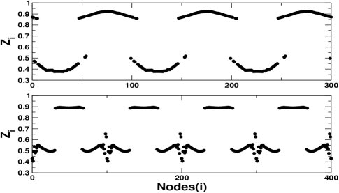
Figure 4: Snapshots for (a) Three layer and (b) Four layer multiplex network. Parameters are $\varepsilon=0.28$ and $r=0.32$. Number of nodes $N=100$ for each layer.

In the absence of any coupling between the nodes ($\varepsilon=0$) or for weak couplings, all the nodes evolve independently and no spatial coherence is observed. For instance, as demonstrated in Fig. 2(a), for $\varepsilon=0.1$ , the evolution of the nodes in the multiplex network yields an incoherent state with no correlations in the neighboring nodes. As the coupling strength is increased, a partially coherent state emerges at $\varepsilon=0.28$ with correlated spatial values of the neighboring nodes in the end and in the middle regions of each layer, however, the spatial range of the incoherent region is more than the coherent region (Fig. 2(b)). This coexistence of the coherent and incoherent dynamics corresponds to the chimera state in the multiplex network.

Figure 5: Spatial entropy as a function of $\varepsilon$. Figure are plotted for $N=100$ and $r=0.32$

The dynamical behaviour of two layers of a multiplex network is a replica of each other manifesting exactly the same spatio-temporal patterns (Fig. 2). Exactly same behaviour is observed for multiplex networks having more than two layers (Fig.4).

At the same coupling value, the spatio-temporal dynamics (Fig. 2 (g)) reflects non-regular skeletal type pattern in the incoherent regions. This irregularity of the pattern suggests that, in the multiplex network framework, a node may get attracted to either of the upper or lower region depending on its initial value as reported for the isolated network [Omelchenko et al. (2011)].

As we increase the coupling strength further, range of the incoherent region decreases as depicted by Fig. 2(c) for $\varepsilon=0.3$. At $\varepsilon=0.4$, we observe a sharp discontinuity in the otherwise smooth profile of $z(j)$ and the incoherency appears at two distinct points in each layer. This is a bifurcation point for the coherent-incoherent transition. Above this coupling value, all the nodes in the multiplex network acquire the complete coherent state as indicated by the appearance of a smooth geometric profile at $\varepsilon=0.44$ (Fig. 2(e)). Fig.2 depicts spatial regions of incoherent nodes and thus indicates a non-zero spatial entropy with the periodic temporal dynamics, representing a Type II chimera state. Further, the regions of incoherence in the spatial profile continues to exist for narrower intervals with an increase in the coupling strength (Fig. 2).

Furthermore, in the Chimera state, the time evolution of all the nodes in the network depict periodic behaviour with the periodicity two depicting temporal regularity. The coupled dynamics displays the spatial chaos which is defined by the non-zero spatial entropy given by $h=d$ $\log_{e}(2)$, where $d$ represents fraction of the incoherent nodes in network [Omelchenko et al. (2011), Coullet et al. (1987)]. We show that the distance measure (Eq.3) is able to easily distinguish between coherent and chimera state. The discontinuous spatial profile (Fig. 3(b)) at $\varepsilon=0.4$ gives rise to the kinks (Fig. 3(d)) in the distance measure distribution signifying transition to the chimera state. We calculate the spatial entropy as a function of the coupling strength ($\varepsilon$) in order to demonstrate the transition between the chimera to the coherent state. A transition from the chimera to coherent state is indicated by the discontinuous change in spatial entropy of the network (Fig.5).

4 Multiplex network versus isolated network

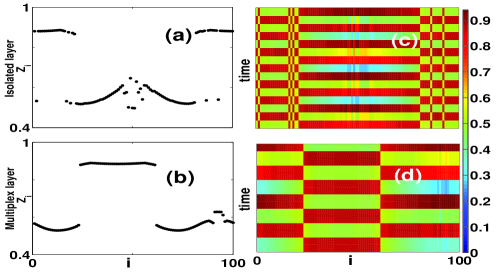
Figure 6: Snapshot and Spatio temporal Pattern for (a,c) Single and (b,d) first $S^{1}$ ring of multiplexed network are shown. Parameters are $\varepsilon=0.30$ and $r=0.32$. Number of nodes $N=100$ for each layer. Initial transient is taken as 5000. results are presented for time range 5000 to 5015.

In order to see the impact of multiplexcity on the dynamical behavior of nodes, we compare the dynamical state of an isolated 1D lattice with that of the multiplexed with another 1D lattice. We find that while the chimera state is retained after multiplexing, the dynamical evolution of the network differs. The multiplexing may enhance or suppress the incoherency. For instance, at $\varepsilon=0.30$, the isolated network displays the chimera state with incoherence in the middle regions of the spatio temporal pattern (Fig. 6 (a) and (c)). After multiplexing, the region of incoherence shrinks to a point discontinuity in the middle and intermediate regions (Fig. 6). Thus, multiplexing here retains the chimera state as well as the type of the chimera state, but leads to a change in the region of incoherence as well as in the dynamical evolution.

5 Sensitivity to initial conditions

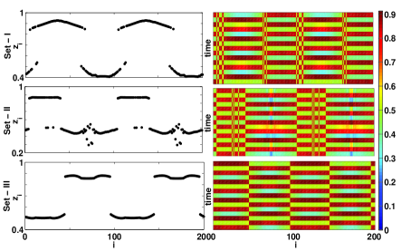
Figure 7: Spatio temporal pattern for multiplex $S^{1}$ rings for different realizations of the initial conditions. Parameters are $\varepsilon=0.32$ and $r=0.32$. Number of nodes $N=100$ for each layer. Initial transient is taken as 5000. results are presented for time range 5000 to 5015.

Furthermore, similar to the isolated networks, in the multiplex networks as well, the chimera exhibits dependency on the initial conditions. As already discussed in the section III, the spatial profile displayed by the chimera state can be very different for different profile of initial conditions for the same set of control parameters, namely $\mu$ and $r$. But interestingly, even for the initial condition given by the same profile as Eq. 4 with a constant value $\sigma$ for a given network size $N$, different realizations of the initial conditions can lead to a different incoherent regions. For example, at $\varepsilon=0.30$, for three different realizations of the initial conditions, all given by Eq. 4, three different spatio temporal patterns are observed (Fig. 7). Though, the multi-chimera state is evident for all the realizations, the region of incoherence differs without any consistent behavior.

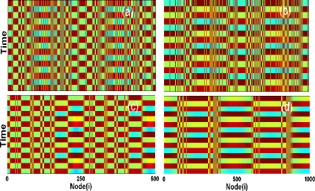
Figure 8: Spatio temporal pattern for multiplex $S^{1}$ rings with coupling strength (a) $\varepsilon=0.21$ (b) $\varepsilon=0.23$ (c) $\varepsilon=0.28$ and (d) $\varepsilon=0.27$ . Coupling range $r=0.32$ and network size for (a),(c) $N=500$ and (b),(d) $N=1000$. Initial transient is taken as 5000. results are presented for time range 5000 to 5015.

Figure 9: Distance measure for multiplex $S^{1}$ ring network. (a),(c) for $\varepsilon=0.44$ and (b),(d) for $\varepsilon=0.41$. Network size $N=500$ and coupling range $r=0.32$ in each layer.

Moreover, we investigated the impact of network size on emergence of chimera state as well as on the critical coupling strength below which one observes incoherent-coherent regime. Fig. 8 presents chimera state for a multiplex ring network with two different network size. For both the network sizes, the coupled evolution exhibits the coexistence of coherence-incoherence dynamics. However, the critical coupling strength for the coherent-incoherent bifurcation increases to $\varepsilon=0.41$ (Fig.9) as compared to $\varepsilon=0.4$ for network size $N=200$ as indicated by Fig. 2.

6 Conclusion

To summarize, we report an emergence of the chimera in the multiplex networks with the layers being represented by 1-d lattice architecture having non-local couplings. We find that an emergence of the chimera is identical in the mirror layers arising due to the underlying symmetry of the network. Furthermore, while the temporal behavior of the network remains periodic even after multiplexing, the range of the coupling strength for which chimera is observed changes. The chimera in the multiplex network is found to be sensitive to the changes in the initial conditions, which is revealed through the changes in the incoherent region of the dynamical evolution for different sets of initial conditions. We also show that the critical coupling strength increases with the size of the network. The results presented here may provide a better understanding to the peculiar nature of the chimera state observed in many natural systems like unihemispheric sleep, ventricular fibrillation, brain networks which incorporates multilayer network architecture [Panaggio & Abrams (2015)].

7 Acknowledgments

SJ is grateful to Department of Science and Technology (DST), Government of India and Council of Scientific and Industrial Research, Government of India project grants EMR/2014/000368 and 25(0205)/12/EMR-II respectively for financial support. SG acknowledges DST, Government of India, for the INSPIRE fellowship (IF150149) as well as the Complex Systems Lab members for timely help and useful discussions. Authors acknowledge Conference on Nonlinear Systems and Dynamics 2015 held at IISER Mohali where this work was initiated.

References

- [Kuramoto & Battogtokh (2002)] Kuramoto,Y. & Battogtokh,D. [2002] “Coexistence of Coherence and Incoherence in Nonlocally Coupled Phase Oscillators,” Nonlinear Phenom. Complex Syst. 380.
- [Abrams & Strogatz (2006)] Abrams,D.M. & Strogatz,S.H. [2006] “Chimera States In a Ring Of Nonlocally Coupled Oscillators,” Int. J. Bifurc. Chaos 16, 21.
- [Sethia et al. (2008)] Sethia,G.C., Sen,A. & Atay,F.M. [2008] “Clustered Chimera States in Delay-Coupled Oscillator Systems,” Phys. Rev. Lett. 100, 144102.
- [Laing (2009)] Laing,C.R. [2009] “The dynamics of chimera states in heterogeneous Kuramoto networks,” Phys. D Nonlinear Phenom. 238, 1569.
- [Omelchenko et al. (2011)] Omelchenko,I., Maistrenko, Y., Hvel, P. & Schll, E. [2011] “Loss of Coherence in Dynamical Networks: Spatial Chaos and Chimera States,” Phys. Rev. Lett. 106, 234102.
- [Hagerstrom et al. (2012)] Hagerstrom, A. M., Murphy, T. E., Roy, R., Hvel, P., Omelchenko I. and Schll E. [2012] “Experimental observation of chimeras in coupled-map lattices,” Nat. Phys. 8 658–661.
- [Larger et al. (2013)] Larger, L., Penkovsky, B. & Maistrenko, Y. [2013] “Virtual Chimera States for Delayed-Feedback Systems,” Phys. Rev. Lett. 111 054103.
- [Abrams et al. (2004))] Abrams, D. M. & Strogatz, S. H. [2004] “Chimera States for Coupled Oscillators,” Phys. Rev. Lett. 93 174102.
- [Maistrenko et al. (2014)] Maistrenko, Y. L., Vasylenko, A., Sudakov, O., Levchenko, R. & Maistrenko, V. L. [2014] “Cascades of Multiheaded Chimera States for Coupled Phase Oscillators,” Int. J. Bifurc. Chaos 24 1440014.
- [Omel’chenko et al. (2012)] Omel’chenko, O. E., Wolfrum, M., Yanchuk, S., Maistrenko, Y. L. & Sudakov, O. [2012] “Stationary patterns of coherence and incoherence in two-dimensional arrays of non-locally-coupled phase oscillators,” Phys. Rev. E. 85 036210.
- [Tinsley et al. (2012)] Tinsley, M. R., Nkomo, S. & Showalter, K. [2012] “Chimera and phase-cluster states in populations of coupled chemical oscillators,” Nat. Phys. 8 662–665.
- [Nkomo et al. (2013)] Nkomo, S., Tinsley, M. R. & Showalter, K. [2013] “Chimera States in Populations of Nonlocally Coupled Chemical Oscillators,” Phys. Rev. Lett. 110 244102.
- [Martens et al. (2013)] Martens, E. A., Thutupalli, S., Fourrire, A. & Hallatschek, O. [2013] “Chimera states in mechanical oscillator networks,” Proc. Natl. Acad. Sci. U. S. A. 110 pp. 10563–10567.
- [Hizanidis et al. (2014)] Hizanidis, J., Kanas, V. G., Bezerianos, A. & Bountis T. [2014] “Chimera States in Networks of Nonlocally Coupled Hindmarsh–Rose Neuron Models,” Int. J. Bifurc. Chaos 24 1450030.
- [Laing (2010)] Laing, C. R. [2010] “Chimeras in networks of planar oscillators,” Phys. Rev. E. 81 066221.
- [Rosin et al. (2014)] Rosin, D. P., Rontani, D., Haynes, N. D., Schll, E. & Gauthier, D. J. [2014] “Transient scaling and resurgence of chimera states in networks of Boolean phase oscillators,” Phys. Rev. E. 90 030902.
- [Rosin (2015)] Rosin,D.P. [2015] Dynamics of Complex Autonomous Boolean Networks (Springer International Publishing, Cham).
- [Lazarides et al. (2015)] Lazarides, N., Neofotistos, G. & Tsironis, G. P. [2015] “Chimeras in SQUID metamaterials,” Phys. Rev. B. 91 054303.
- [Omel’chenko et al. (2008)] Omel’chenko, O. E., Maistrenko, Y. L. & Tass, P. A. [2008] “Chimera States: The Natural Link Between Coherence and Incoherence,” Phys. Rev. Lett. 100 044105.
- [Sheeba et al. (2010)] Sheeba, J. H., Chandrasekar, V. K. & Lakshmanan, M. [2010] “Chimera and globally clustered chimera: Impact of time delay,” Phys. Rev. E. 81 046203.
- [Schmidt et al. (2014)] Schmidt, L., Schnleber, K., Krischer, K. & Garca-Morales, V. [2014] “Coexistence of synchrony and incoherence in oscillatory media under nonlinear global coupling,” Chaos 24 013102.
- [Yeldesbay et al. (2014)] Yeldesbay, A., Pikovsky, A. & Rosenblum, M. [2014] “Chimeralike States in an Ensemble of Globally Coupled Oscillators,” Phys. Rev. Lett. 112 144103.
- [Buscarino et al. (2015)] Buscarino, A., Frasca, M., Gambuzza, L. V. & Hvel, P. [2015] “Chimera states in time-varying complex networks,” Phys. Rev. E. 91 022817.
- [Laing (2015)] Laing,C. R. [2015] “Chimeras in networks with purely local coupling,” Phys. Rev. E. 92, 050904(R)
- [Xie et al. (2014)] Xie, J., Knobloch, E. & Kao, H. C. [2014] “Multicluster and traveling chimera states in nonlocal phase-coupled oscillators,” Phys. Rev. E. 90 022919.
- [Omelchenko et al. (2013)] Omelchenko, I., Omel’chenko, O. E., Hvel, P. & Schll E. [2013] “When Nonlocal Coupling between Oscillators Becomes Stronger: Patched Synchrony or Multichimera States,” Phys. Rev. Lett., 110 224101.
- [Abrams et al. (2008)] Abrams,D.M., Mirollo,R., Strogatz, S.H. & Wiley,D.A. [2008] “Solvable Model for Chimera States of Coupled Oscillators,” Phys. Rev. Lett. 101 084103.
- [Panaggio & Abrams (2015)] Panaggio, M. J. & Abrams D. M. [2015] “Chimera states on the surface of a sphere,” Phys. Rev. E. 91 022909.
- [Semenova et al. (2015)] Semenova,N., Zakharova, A., Schll,E. & Anishchenko,V. [2015] “Does hyperbolicity impede emergence of chimera states in networks of nonlocally coupled chaotic oscillators?,” EPL 112 40002.
- [Dutta & Banerjee (2015)] Dutta,P. S. & Banerjee,T. [2015] “Spatial coexistence of synchronized oscillation and death: A chimeralike state,” Phys. Rev. E. 92 042919
- [Wolfrum et al. (2011)] Wolfrum, M., Omel’chenko, O. E., Yanchuk, S. & Maistrenko, Y. L. [2011] “Spectral properties of chimera states,” Chaos 21 013112.
- [Omelchenko et al. (2012)] Omelchenko, I., Riemenschneider, B., Hvel, P., Maistrenko, Y. L. & Schll, E. [2012] “Transition from spatial coherence to incoherence in coupled chaotic systems,” Phys. Rev. E. 85 026212.
- [Zakharova et al. (2014)] Zakharova, A., Kapeller, M. & Schll, E. [2014] “Chimera Death: Symmetry Breaking in Dynamical Networks,” Phys. Rev. Lett. 112 154101.
- [Boccaletti et al. (2014)] Boccaletti S. et al. [2014] “The structure and dynamics of multilayer networks,” Phys. Rep. 544 pp 1–122.
- [Lee et al. (2012)] Lee, K. M., Kim, J. Y., Cho, W., Goh K. I. & Kim, I. M. [2012] “Correlated multiplexity and connectivity of multiplex random networks,” New J. Phys. 14 033027.
- [Wang et al. (2015)] Wang, Z., Wang, L., Szolnoki, A. & Perc, M. [2015] “Evolutionary games on multilayer networks: a colloquium,” Eur. Phys. J. B 88 124.
- [Kivelä et al. (2014)] Kivelä, M. et al. [2014] “Multilayer Networks,” Journal of Complex Networks 2 3 pp 203–271.
- [Jacobson (2009)] Jacobson, N. [2009] Basic Algebra I (Dover Publications).
- [Panaggio & Abrams (2015)] Panaggio, M. J. & Abrams D. M. [2015] “Chimera states: coexistence of coherence and incoherence in networks of coupled oscillators,” Nonlinearity 28 R67–87.
- [Coullet et al. (1987)] Coullet, P., Elphick, C. & Repaux D. [1987] “Nature of Spatial Chaos,” Phys. Rev. Lett. 58 431.