Aperiodic Crystals and Beyond

Abstract

Crystals are paradigms of ordered structures. While order was once seen as synonymous with lattice periodic arrangements, the discoveries of incommensurate crystals and quasicrystals led to a more general perception of crystalline order, encompassing both periodic and aperiodic crystals. The current definition of crystals rests on their essentially point-like diffraction. Considering a number of recently investigated toy systems, with particular emphasis on non-crystalline ordered structures, the limits of the current definition are explored.

1 What is order?

The human brain is very skilled at detecting patterns and recognising order in a structure, and ordered structures permeate cultural achievements of human civilisations, be it in the arts, architecture or music. The ability to detect and describe patterns is also at the basis of all scientific enquiry; see Mumford & Desolneux (2010) for more on pattern theory. It may thus be surprising that a concept as fundamental as order does not have any well-defined precise meaning, and that it appears to be rather challenging to come up with a proper definition of what constitutes order in a structure. As a consequence, there currently is no satisfactory measure to quantify order in any given spatial structure.

There are two common approaches to tackle this issue. One is to employ diffraction, which effectively measures two-point correlations in the structure; see Cowley (1995) for background. For kinematic diffraction, in the far-field approximation, the diffraction measure is the Fourier transform of the autocorrelation (or Patterson) function. Diffraction is the approach taken to characterise crystalline materials. The current definition of a crystal, which is based on its diffraction, derives from a definition which first appeared in the terms of reference of the IUCr Commission on Aperiodic Crystals, published in the 1991 report of the IUCr Executive Committee (International Union of Crystallography, 1992, p. 928); in fact, it is less general than what the commission proposed. The following quotes the more specific definition given in Authier and Chapuis (2014), and used in the IUCr Online Dictionary of Crystallography.

A material is a crystal if it has essentially a sharp diffraction pattern. The word essentially means that most of the intensity of the diffraction is concentrated in relatively sharp Bragg peaks, besides the always present diffuse scattering. In all cases, the positions of the diffraction peaks can be expressed by

$$\mathbf{H}\,=\sum_{i=1}^{n}h_{i}\,\mathbf{a}_{i}^{*}\qquad(n\geq 3).$$ (1)

Here $\mathbf{a}_{i}^{*}$ and $h_{i}$ are the basis vectors of the reciprocal lattice and integer coefficients respectively and the number $n$ is the minimum for which the positions of the peaks can be described with integer coefficient $h_{i}$.

The conventional crystals are a special class, though very large, for which $n=3$.

The prominent role of the word essentially shows that this is a humble definition, in the sense that it reflects our limited knowledge of the structures we may potentially encounter in nature. The interpretation given in the definition that ‘essentially’ means that most of the intensity is concentrated in Bragg peaks means that the integrated contribution from the background must be weak compared to the Bragg diffraction, which is rather arbitrary, as any Bragg diffraction indicates order. By allowing the integer $n$ to be larger than the three space dimensions we live in, aperiodic crystals are included in this definition, and conventional (periodic) crystals have become a special class (for which $n=3$). Note that $n$ is restricted to be finite here, so this particular form of the definition excludes pure point diffractive systems with non-finitely generated Fourier modules (over integer coefficients); the definition stipulates that Bragg peaks in crystals can be indexed by a finite number of integer coefficients. Note that the definition originally proposed in 1991 did not include this restriction (International Union of Crystallography, 1992, p. 928).

Because the inverse problem of diffraction is inherently difficult (Bombieri & Taylor, 1986) and, in general, not unique (Patterson, 1944), we do not have a complete characterisation of structures that show pure point diffraction (which means that the diffraction consists of Bragg peaks only), even in the idealised case of an ideal, perfect structure. Neither do we have a good understanding of what structures with an essentially pure point spectrum may look like.

The second approach, which is particularly suited to stochastic systems, employs the entropy of a structure. Entropy takes into account the number of different local configurations of a system, and how this number grows with the system size; normally you are looking at an exponential growth with the system size, and any sub-exponential growth corresponds to zero entropy. Clearly, entropy can distinguish deterministic from random systems, and looking at different forms of scaling behaviour makes it possible to differentiate, at least to some extent, between different degrees of disorder. However, any deterministic structure has zero entropy (as has any sufficiently small deviation from it), so entropy is a rather crude measure of order.

In this article, the current state of knowledge of mathematical diffraction of structures is summarised and discussed in relation with our notion of crystalline order. The current article attempts to present a broad overview only; for details on calculations and further background, we refer to recent survey articles (Baake & Grimm 2011a, Baake & Grimm 2012) and to the monograph by Baake & Grimm (2013), as well as to references therein. Using a number of explicit example structures with different types of diffraction spectrum, the range of possibilities is explored, contributing to the ongoing discussion on what order means in crystals and beyond (van Enter & Miȩkisz 1992, Lifshitz 2003, 2007, 2011).

2 Mathematical diffraction

In 2014, we were celebrating the international year of crystallography, and were looking back at a century of rapid developments in crystallography since von Laue (Friedrich, Knipping & von Laue 1912, von Laue 1912) and father and son Bragg (Bragg & Bragg 1913) first employed X-ray diffraction to analyse the atomic structure of crystalline materials; see Authier (2013) for a historical account. In the simplest setting, which is suitable in particular for X-ray diffraction, it is sufficient to describe the kinematic scattering of radiation by the sample, and consider the far-field (Fraunhofer) limit for the outgoing radiation. The calculation of the diffraction pattern of a given structure then becomes possible by means of harmonic analysis, while the corresponding inverse problem of determining a structure from its pattern of diffraction intensities is, in general, difficult and non-unique, even in this simplified setting. This section attempts to present a summary of mathematical diffraction theory, highlighting the ideas and the flavour of the approach without going into technicalities, while trying to explain some of the technical terms by means of simple examples and familiar notions; for mathematical details, the reader is referred to Baake & Grimm (2013).

2.1 What is a measure?

A mathematically satisfactory approach to describe extended (infinite) systems, such as ideal crystals, is provided by using measures to describe both the distribution of matter in the scattering medium and the distribution of scattered radiation intensity in space. In mathematics, measures are the natural concept to quantify spatial distributions, and are related to the notion of integration. The general approach to measures in mathematics is rather technical, but there is a simpler way to think of measures (which is due to a result called the Riesz-Markov representation theorem; see Reed & Simon (1980) for details). Indeed, it is possible to regard a measure as a linear functional, which is a linear map that associates a number to each function from an appropriate space. A familiar example is the integral of a function, which is the example we start with.

A well-known and widely used measure in mathematics is Lebesgue measure, which is commonly used in integration of functions on the real numbers $\mathbb{R}$. We denote Lebesgue measure by the letter $\lambda$. If $f\!:\;x\mapsto f(x)$ is a function on $\mathbb{R}$, the Lebesgue measure of $f$ is

$$\lambda(f)\,=\,\int_{\mathbb{R}}f(x)\,\mathrm{d}\lambda(x)\,=\,\int_{\mathbb{R}}f(x)\,\mathrm{d}x\,,$$

where the usual shorthand $\mathrm{d}x$ is used for integration with respect to Lebesgue measure. So Lebesgue measure associates to a function $f$ a number, which is its integral.

The Lebesgue measure of a set $A\subset\mathbb{R}$, written as $\lambda(A)$, is given by

$$\lambda(A)\,=\,\lambda(1_{A})\,=\,\int_{\mathbb{R}}1_{A}(x)\,\mathrm{d}x\,=\,\int_{A}\mathrm{d}x\,=\,\mathrm{vol}(A)\,,$$

where $1_{A}$ is the characteristic function (or indicator function) of $A$, which takes the value $1_{A}(x)=1$ for all $x\in A$, and $1_{A}(x)=0$ otherwise. The Lebesgue measure of a set is what we call the volume (as in this case we are in one dimension, the volume is a length); for instance, the Lebesgue measure of the interval $I=[a,b]$ with $b\geq a$ is $\lambda(I)=\lambda([a,b])=b-a$. Lebesgue measure is the unique translation-invariant measure on $\mathbb{R}$ (meaning that $\lambda(A)=\lambda(A+t)$ for any translation $t\in\mathbb{R}$) that assigns the volume $1$ to the unit interval $[0,1]$. Lebesgue measure on $\mathbb{R}$ generalises in the familiar way to $d$-dimensional space $\mathbb{R}^{d}$, corresponding to $d$-dimensional (multiple) integrals. For simplicity, we will mainly consider the case $d=1$ in what follows.

Another well-known and important measure is the Dirac measure (or point measure) at a point $x\in\mathbb{R}$, denoted by $\delta_{x}$. It describes a localised structure at a point $x$ in space, with total measure $1$. This means that, if $f$ is a function on $\mathbb{R}$, its point measure at $x$ is $\delta_{x}(f)=f(x)$. In the physics literature, the point measure is often written like a function $\delta(x)$ (which can be considered a generalised function or distribution obtained as a limit of functions, for instance of a sequence of Gaussian functions of integral $1$, centred at the origin, and with a decreasing width, which then become increasingly sharper), with the suggestive notation

$$\delta_{x}(f)\,=\,\int_{\mathbb{R}}f(y)\,\delta(x-y)\,\mathrm{d}y\,=\,f(x)\,.$$

This notation can be used consistently as long as one remembers that Dirac’s $\delta$ is not a function in the usual sense. As above, one can also define the point measure of a set $A\subset\mathbb{R}$, which is $\delta_{x}(A)=\delta(1_{A})=1_{A}(x)$, so $\delta_{x}(A)=1$ if $x\in A$ and $0$ otherwise.

2.2 Dirac combs

Point measures are often used to describe a set of localised scatterers in space. Given a set of scatterers located at points in a subset $\varLambda\subset\mathbb{R}$ (which we usually assume to be a Delone set, which means that it neither contains points that are arbitrarily close to each other nor holes of arbitrary size), we can associate a measure

$$\delta_{\varLambda}\,:=\,\sum_{x\in\varLambda}\delta_{x}$$

which we call the Dirac comb (a term coined by de Bruijn (1986); see also Córdoba (1989)) of $\varLambda$. An example of such a Dirac comb is $\delta_{\mathbb{Z}}=\sum_{n\in\mathbb{Z}}\delta_{n}$, which is the uniform Dirac comb on the integer lattice.

By introducing scattering weights $w(x)$ at position $x\in\mathbb{R}$ (which in general can be complex numbers, but we will assume to be real for the purpose of this exposition), we arrive at a weighted Dirac comb

$$\omega\,=\,w\,\delta_{\varLambda}\,=\,\sum_{x\in\varLambda}w(x)\,\delta_{x}\,,$$ (2)

which can serve as a model representing a scattering medium containing different types of scatterers. Any measure of this type, consisting of a (weighted) sum of point measures, is called a pure point measure (with respect to Lebesgue measure). It is possible to include realistic scattering profiles by considering convolutions with appropriate motives, so this approach is not as restrictive as it may seem. A schematic representation of an example, the weighted (periodic) Dirac comb

$$\omega\,=\,\delta_{\mathbb{Z}}+\tfrac{1}{2}\,\delta_{\mathbb{Z}+\frac{1}{2}}+\tfrac{1}{4}\,\delta_{\mathbb{Z}+\{\frac{1}{4},\frac{3}{4}\}}$$ (3)

is shown in Figure 1.

Figure 1: Schematic representation of the weighted (periodic) Dirac comb $\omega$ of Eq. (3). Point measures $a\,\delta_{x}$ are represented as columns at position $x$ of height proportional to their weight $a$.

Attaching scattering profiles to a Dirac comb is one way to represent a continuous scattering intensity in space. Of course, there is a more direct approach if the scattering intensity is described by a continuous distribution is space. If $\varrho$ is a such a continuous (or, at least, locally integrable) function on $\mathbb{R}$, it defines a measure $\mu$ on $\mathbb{R}$ via

$$\mu(f)\,=\,\int_{\mathbb{R}}f(x)\,\mathrm{d}\mu(x)\,=\,\int_{\mathbb{R}}f(x)\,\varrho(x)\,\mathrm{d}x\,.$$

In this case $\varrho$ is called the density of the measure $\mu$. Any measure $\mu$ that can be written in this form is called an absolutely continuous measure (with respect to Lebesgue measure).

The measures we are interested in are those which describe distributions (of scatterers or scattering intensity) in space, and one physical restriction we would like to impose is that any finite region of space can only contain a finite total scattering strength or finite intensity. The measures that satisfy this property are called translation bounded measures. A Dirac comb $\delta_{\varLambda}$ of a Delone set $\varLambda\subset\mathbb{R}$ is always translation bounded, because there can be only finitely many points in any finite region of space, due to the minimum distance between points. The same is true for a weighted Dirac comb provided that the weight function $w(x)$ is bounded. An examples of a measure that is not translation bounded would be a Dirac comb of a point set with an accumulation point, for instance $\sum_{n\in\mathbb{Z}\setminus\{0\}}\delta_{1/n}$. For this measure, any interval containing the origin contains infinitely many point measures, and thus has infinite measure.

2.3 Lebesgue decomposition

A central result in measure theory is Lebesgue’s decomposition theorem. It states that any measure can be written as a sum of three components in a unique way (with respect to a reference measure, which is our case will always be Lebesgue measure). If $\mu$ is a measure on $\mathbb{R}$, the three components are denoted as

$$\mu\,=\,\mu_{\mathsf{pp}}+\mu_{\mathsf{sc}}+\mu_{\mathsf{ac}}$$

and are called the pure point component $\mu_{\mathsf{pp}}$, the singular continuous component $\mu_{\mathsf{sc}}$ and the absolutely continuous component $\mu_{\mathsf{ac}}$. We have met typical examples of pure point and absolutely continuous measures above, so the obvious question is what a singular continuous measure looks like. As it is defined, it is all that is ‘left’ if you remove the pure point part (consisting of a sum of weighted point measures) and the absolutely continuous part (which is described by a locally integrable density function) — but this does not really help to gain an understanding of what such a measure represents. Singular continuous measures are rather weird objects indeed; they do not give weight to any single point in space (because otherwise it would have a pure point component), but are concentrated on sets of vanishing volume (because otherwise you could describe part of it by a density function).

Figure 2: Sketch of the classic middle thirds Cantor set construction (inset) and the ‘Devil’s staircase’ distribution function $F$ of the corresponding singular continuous measure.

The best-known example of a singular continuous measure is provided by the classic middle-thirds Cantor set; see Figure 2. Starting from the unit interval, the Cantor set is constructed by removing the middle third of it, then removing the middle thirds of the two resulting intervals, and iterating this procedure ad infinitum. The corresponding Cantor measure is constructed by starting from the Lebesgue measure on the interval, so we have total measure $1$, and at each step distributing the mass equally onto the constituent intervals. In the limit, the total measure is thus still $1$, but there is neither any isolated point that carries a finite measure (since the measure of each interval in the $n$th step is $2^{-n}$, so it vanishes in the limit) nor any interval of finite length that is in the support of the measure (meaning that the measure does not vanish on it). The measure constructed in this way is thus singularly continuous, and can be described in terms of a distribution function which is a ‘Devil’s staircase’. This function is constant almost everywhere, and displays a hierarchy of plateaux in its graph (see Figure 2) which reflect the hierarchy of gaps produced by the excision steps in the Cantor construction. This function plays the role of the integrated density for the singular continuous measure.

Lebesgue’s decomposition provides a rigorous way to separate the diffraction measure of a structure into its pure point (Bragg) part and its singular and absolutely continuous components. However, using this as the definition really only makes sense if one works with infinite systems (because finite systems will always have absolutely continuous diffraction). This is similar in spirit to the definition of a phase transition in materials (as a discontinuity in a thermodynamic potential), which again only applies in the mathematically rigorous sense to an infinite system (because for finite systems these potentials are smooth functions). Nevertheless, these concepts have proved useful for applications to macroscopically large (albeit finite) systems.

2.4 Autocorrelation and diffraction

A key quantity in diffraction theory is the autocorrelation, which quantifies the two-point correlation of a structure. In crystallography, this is often called the Patterson function. If the material is described by a (real) density function $\varrho$ on $\mathbb{R}$ (so we deal with an absolutely continuous distribution), the autocorrelation is an absolutely continuous measure whose density is the familiar convolution

$$P(x)\,=\,\int_{\mathbb{R}}\varrho(y)\,\varrho(y+x)\,\mathrm{d}x\,=\,\bigl{(}\varrho*\widetilde{\varrho}\bigr{)}(x)\,,$$

where $\widetilde{\varrho}$ is the function defined by $\widetilde{\varrho}(x)=\varrho(-x)$.

In the case that the material is described by a one-dimensional weighted Dirac comb $\omega$ of the form given in Eq. (2) (with real weight function $w(x)$), the autocorrelation is a pure point measure

$$\gamma\,=\,\sum_{z\in\varLambda-\varLambda}\eta(z)\,\delta_{z}\,,$$

with non-vanishing contributions only at distances $z$ in the difference set $\varLambda-\varLambda=\{x-y\mid x,y\in\varLambda\}$ (which you may interpret as the set of interatomic distances). The point masses for interatomic distances $z$ are weighted by the autocorrelation coefficients $\eta(z)$, which are given by

$$\eta(z)\,=\,\lim_{R\to\infty}\frac{1}{2R}\sum_{\begin{subarray}{c}|x|\leq R,x\in\varLambda\\ z-x\in\varLambda\end{subarray}}w(x)\,w(z-x)\,,$$

provided that these limits exist. Note that $2R$ is the length of the interval $(-R,R)$, so the autocorrelation coefficient $\eta(z)$ is precisely the volume-averaged two-point correlation for the interatomic distance $z$.

Using the language of measures, these equations can be neatly summarised as follows. Given a (translation bounded) real measure $\omega$, again for simplicity in one dimension, its autocorrelation measure $\gamma$ is defined as

$$\gamma\,=\,\omega\circledast\widetilde{\omega}\,:=\lim_{R\to\infty}\frac{\;\omega|_{R}\ast\widetilde{\omega|_{R}}\;}{2R},$$ (4)

provided the limit exists. Here, $\omega|_{R}$ denotes the restriction of $\omega$ to the interval $(-R,R)$, and $\widetilde{\mu}$ is defined via $\widetilde{\mu}(g)=\mu(\widetilde{g})$ with $\widetilde{g}(x)=\overline{g(-x)}$ as above. Finally, $\ast$ denotes the standard convolution of measures, which is the appropriate generalisation of the convolution of functions. The autocorrelation of $\omega$ is thus the volume-averaged convolution $\circledast$ (also called the Eberlein convolution) of $\omega$ with its ‘flipped-over’ version $\widetilde{\omega}$, and thus picks out the two-point correlations in the structure described by $\omega$. This approach to mathematical diffraction was pioneered by Hof (1995).

The diffraction measure is then the Fourier transform $\widehat{\gamma}$ of the autocorrelation, so essentially it provides a spectral analysis for the two-point correlations in the original structure. It is a translation bounded, positive measure, which quantifies how much of the kinematic scattering intensity reaches a given volume in space. Lebesgue’s decomposition

$$\widehat{\gamma}\;=\;\widehat{\gamma}_{\mathrm{pp}}+\widehat{\gamma}_{\mathrm{sc}}+\widehat{\gamma}_{\mathrm{ac}}$$

into its pure point part (the Bragg peaks, of which there are at most countably many), its absolutely continuous part (the diffuse background scattering, described by a locally integrable density function) and its singular continuous part (which encompasses anything that remains) provides a mathematically rigorous definition of the different types of diffraction. For the definition of a crystal cited above, it is the pure point part $\widehat{\gamma}_{\mathrm{pp}}$ that matters — a crystal is a structure where this part represents the majority of the diffracted intensity (there will always be some continuous diffraction in practice), though this alone does not guarantee that the positions of Bragg peaks can be indexed by a finite number of integers. Indeed, there are examples of systems that are pure point diffractive, meaning that $\widehat{\gamma}=\widehat{\gamma}_{\mathrm{pp}}$, where this is not the case; we shall meet an example below.

3 Periodic crystals

A conventional, periodic crystal is described as a lattice-periodic structure, corresponding to an ideal infinite crystal without defects or surfaces. A periodic crystal is characterised by its periods (translations that keep the crystal invariant), which form a lattice $\varGamma$ (because any linear combinations of periods are also periods), and by the distribution of scatterers in a unit cell (fundamental domain) of this lattice. Here, a lattice $\varGamma$ in $d$-dimensional space is the set of integer linear combinations of $d$ linearly independent basis vectors, so it can be written in the form

$$\varGamma\,:=\,\left\{\textstyle\sum_{i=1}^{d}a_{i}v_{i}\mid a_{i}\in\mathbb{Z}\right\},$$

where $v_{i}\in\mathbb{R}^{d}$, for $1\leq i\leq d$, are linearly independent vectors in $\mathbb{R}^{d}$. Familiar examples are the integer lattice $\mathbb{Z}$ in one dimension, the square lattice $\mathbb{Z}^{2}$ in two dimensions and the simple (primitive) cubic lattice $\mathbb{Z}^{3}$ in three dimensions.

If the scattering medium has a (periodic) crystal structure described by a lattice $\varGamma$, it can always be represented as a measure

$$\omega\,=\,\mu\ast\delta_{\varGamma}\,,$$ (5)

where $\mu$ can be chosen as a finite measure which describes the decoration of the fundamental domain, while the Dirac comb $\delta_{\varGamma}$ ensures lattice periodicity.

The corresponding autocorrelation measure is a $\varGamma$-periodic measure that can be calculated from the appropriate generalisation of Eq. (4) as

$$\gamma\,=\,\mathrm{dens}(\varGamma)\,(\mu\ast\widetilde{\mu})\ast\delta_{\varGamma}\,,$$ (6)

using $\widetilde{\delta_{\varGamma}}=\delta_{\varGamma}$ and $\delta_{\varGamma}\circledast\delta_{\varGamma}=\mathrm{dens}(\varGamma)\,\delta_{\varGamma}$, where $\mathrm{dens}(\varGamma)$ denotes the density (per unit volume) of the lattice $\varGamma$. The diffraction measure $\widehat{\gamma}$ is then given by

$$\widehat{\gamma}\,=\,\bigl{(}\mathrm{dens}(\varGamma)\bigr{)}^{2}\,\big{|}\widehat{\mu}\big{|}^{2}\,\delta_{\varGamma^{*}}\,.$$ (7)

This provides the familiar result for periodic crystals: Any perfect periodic crystal with lattice of periods $\varGamma$ shows pure point diffraction with Bragg peaks located on the reciprocal lattice $\varGamma^{*}$, and the intensity of the Bragg peak is determined by the density of the crystal lattice $\varGamma$ and by the continuous function $\big{|}\widehat{\mu}\big{|}^{2}$, which depends on the distribution of scatterers in a fundamental domain of $\varGamma$. By expressing the reciprocal lattice positions as linear combinations of basis vectors of the reciprocal lattice $\varGamma^{*}$, this can be cast in the form of Eq. (1) with $n=d$.

As a one-dimensional example, consider the weighted Dirac comb $\omega$ of Eq. (3) and Figure 1. It can be written as

$$\omega\,=\,\left(\delta_{0}+\tfrac{1}{4}\,\delta_{\frac{1}{4}}+\tfrac{1}{2}\,\delta_{\frac{1}{2}}+\tfrac{1}{4}\,\delta_{\frac{3}{4}}\right)*\delta_{\mathbb{Z}}\,,$$

so here $\mu=\delta_{0}+\frac{1}{4}\delta_{\frac{1}{4}}+\frac{1}{2}\delta_{\frac{1}{2}}+\frac{1}{4}\delta_{\frac{3}{4}}$ describes the four scatterers within the fundamental domain $[0,1)$ of the lattice $\varGamma=\mathbb{Z}$. Note that in this case we have

$$\widetilde{\omega}\,=\,\left(\delta_{0}+\tfrac{1}{4}\,\delta_{-\frac{1}{4}}+\tfrac{1}{2}\,\delta_{-\frac{1}{2}}+\tfrac{1}{4}\,\delta_{-\frac{3}{4}}\right)*\delta_{\mathbb{Z}}\,=\,\omega\,,$$

due to the equivalence of positions differing by integers in the periodic lattice and the symmetric distributions of scatterers in the fundamental domain. Let us now calculate the autocorrelation and diffraction of this comb.

Clearly, since all distances are multiples of $\frac{1}{4}$, the autocorrelation in this case will have a similar form as the comb $\omega$ itself, just with different coefficients, which are given by summing up the products of the weights of scatterers with a given separation. To obtain these coefficients, one can compute the convolution of $\omega$ with itself (or equivalently of $\mu$ with itself) term by term, using the relation $\delta_{x}*\delta_{y}=\delta_{x+y}$. This gives

$$\gamma\,=\,\left(\tfrac{11}{8}\,\delta_{0}+\tfrac{3}{4}\,\delta_{\frac{1}{4}}+\tfrac{9}{8}\,\delta_{\frac{1}{2}}+\tfrac{3}{4}\,\delta_{\frac{3}{4}}\right)*\delta_{\mathbb{Z}}\,.$$

For instance, the coefficient $\frac{11}{8}=1^{2}+(\frac{1}{4})^{2}+(\frac{1}{2})^{2}+(\frac{1}{4})^{2}$ of $\delta_{0}$ comes from adding up the contributions to integer distances. A schematic presentation of the autocorrelation $\gamma$ is shown in Figure 3.

The corresponding diffraction measure $\widehat{\gamma}$ is obtained by taking the Fourier transform, using that $\widehat{a\delta_{x}}=a\mathrm{e}^{2\pi\mathrm{i}kx}$. This gives

$$\begin{split}\widehat{\gamma}\,&=\,\left(\tfrac{11}{8}+\tfrac{9}{8}(-1)^{k}+\tfrac{3}{2}\cos(\tfrac{\pi k}{2})\right)*\delta_{\mathbb{Z}}\\ &=\,4\,\delta_{4\mathbb{Z}}+\delta_{4\mathbb{Z}+2}+\tfrac{1}{4}\,\delta_{4\mathbb{Z}+\{1,3\}}\,.\end{split}$$

The diffraction pattern is thus periodic, but with period $4$ (due to the smallest distance between scatterers being $\frac{1}{4}$). A schematic picture of the diffraction pattern is shown in Figure 3.

Figure 3: Schematic representation of the autocorrelation (top) and diffraction (bottom) of the weighted Dirac comb $\omega$ of Eq. (3) and Figure 1.

As a second example, consider a two-dimensional crystal with lattice of periods $\varGamma=\mathbb{Z}^{2}$, with two scatterers (of unit scattering strength) per unit cell, one placed at lattice points and the other at an arbitrary position $(a,b)\in[0,1)^{2}$. The corresponding point set is $\varLambda=\mathbb{Z}^{2}\cup\bigl{(}\mathbb{Z}^{2}+(a,b)\bigr{)}$, and the Dirac comb can be written as $\omega=\varrho*\delta_{\mathbb{Z}^{2}}=(\delta_{0,0}+\delta_{a,b})*\delta_{\mathbb{Z}^{2}}$. Its autocorrelation is

$$\begin{split}\gamma&\,=\,\bigl{(}\varrho*\widetilde{\varrho}\bigr{)}*\delta_{\mathbb{Z}^{2}}\\ &\,=\,(\delta_{(0,0)}+\delta_{(a,b)})*(\delta_{(0,0)}+\delta_{-(a,b)})*\delta_{\mathbb{Z}^{2}}\\ &\,=\,\bigl{(}2\,\delta_{(0,0)}+\delta_{(a,b)}+\delta_{-(a,b)}\bigr{)}*\delta_{\mathbb{Z}^{2}}.\end{split}$$

The corresponding diffraction measure is then

$$\begin{split}\widehat{\gamma}&\,=\,\lvert\widehat{\varrho}\,\rvert^{2}(k,\ell)\,\delta_{\mathbb{Z}^{2}}\\ &\,=\,\bigl{(}2+2\,\mathrm{Re}(\mathrm{e}^{-2\pi\mathrm{i}(ka+\ell b)})\bigr{)}\,\delta_{\mathbb{Z}^{2}}\\ &\,=\,\left(2+2\cos\bigl{(}(2\pi(ka+\ell b)\bigr{)}\right)\,\delta_{\mathbb{Z}^{2}}\\ &\,=\,\left(2\cos\bigl{(}\pi(ka+\ell b)\bigr{)}\right)^{2}\,\delta_{\mathbb{Z}^{2}}\end{split}$$

for $k,\ell\in\mathbb{Z}$. Note that, while the diffraction measure is supported on $\mathbb{Z}^{2}$ as expected (as $\mathbb{Z}^{2}$ is self-dual), it need not have any non-trivial period. In fact, $\widehat{\gamma}$ is periodic in one or two directions precisely if one or both coordinates $a$ and $b$ are rational, respectively; an example with one periodic direction is shown in Figure 4. Although the positions of Bragg spots for a lattice-periodic structure are again lattice-periodic, in general the intensities will not respect the periodicity of the dual lattice.

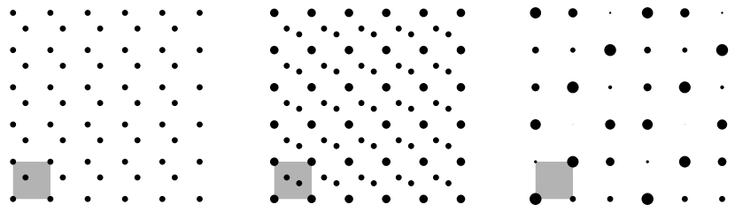
Figure 4: The left panel shows a schematic representation of the two-dimensional toy crystal discussed in the text, with two scatterers of equal strength at positions $(0,0)$ and $(a,b)=(\frac{1}{3},\frac{1}{\sqrt{3}})$ of the fundamental domain (indicated by shading). The corresponding autocorrelation $\gamma$ is shown in the central panel, while the corresponding diffraction measure $\widehat{\gamma}$ is displayed in the right panel. Here, a point measure is represented by a dot that is centred at the position of the peak and has an area proportional to the weight of the point measure. The irrational position in the vertical direction leads to an incommensurate modulation of the peak intensities in this direction, which the diffraction is periodic with period $3$ in the horizontal direction.

4 Aperiodic crystals

The arguably best understood class of aperiodic structures are cut and project sets, also called model sets. Model sets can be viewed as a natural generalisation of the notion of quasiperiodic functions, which goes back to Harald Bohr (1947), and were first introduced by Yves Meyer (1972) in the context of harmonic analysis. The basic idea of the construction is to obtain an aperiodic structure as a suitable ‘slice’ of a higher-dimensional periodic lattice, which is then projected onto a suitable space of the desired dimension. For simplicity, we mainly consider the case where the higher-dimensional space is a Euclidean space of the form $\mathbb{R}^{d+m}$, with $\mathbb{R}^{d}$ being the physical space (sometimes also called the direct or the parallel space) that hosts the aperiodic structure (so $1\leq d\leq 3$ for physically relevant cases), and $\mathbb{R}^{m}$ the internal (or perpendicular) space which is used in the construction.

Let us start with an example, where $d=m=1$. In this case, we are projecting a one-dimensional aperiodic structure from a two-dimensional (periodic) lattice. In this example, the lattice $\mathcal{L}$ is given by all integer linear combinations of two basis vectors, which we choose as $(1,1)$ and $(\tau,1-\tau)$, where $\tau=(1+\sqrt{5})/2$ is the golden ratio, so we have

$$\mathcal{L}\,=\,\mathbb{Z}\,(1,1)+\mathbb{Z}\,(\tau,1-\tau)\,=\,\bigl{\{}m\,(1,1)+n\,(\tau,1-\tau)\;\big{|}\;m,n\in\mathbb{Z}\bigr{\}}\,.$$

The lattice points are shown as black dots in Figure 5. The lattice is oriented such that the horizontal space along the $(1,0)$ direction is the physical space and the vertical direction along $(0,1)$ corresponds to the internal space. We call the projection to the physical space $\pi$, and the projection to the internal space $\pi_{\mathrm{int}}$. The projections of all lattice points $L=\pi(\mathcal{L})$ to physical space and $L^{\star}=\pi_{\mathrm{int}}(\mathcal{L})$ to internal space are both dense in their corresponding one-dimensional spaces. The set $L$ is explicitly given by $L=\mathbb{Z}[\tau]=\{m+n\tau\mid m,n\in\mathbb{Z}\}$, so all integer combinations of multiples of $1$ and $\tau$, which is dense because $\tau$ is irrational, and $L^{\star}$ has the same form. Note that the projections are one-to-one in both directions. In particular, any point in $L$ corresponds to a uniquely defined point in $\mathcal{L}$. In fact, $\pi^{-1}(x)=(x,x^{\star})$, where the $\star$-map is defined by mapping $1$ to $1$ and $\tau$ to $1-\tau$ (which corresponds to the ‘algebraic conjugation’ $\sqrt{5}\mapsto-\sqrt{5}$), so $(m+n\tau)^{\star}=m+n(1-\tau)=m+n-n\tau$ for all $m,n\in\mathbb{Z}$.

The final ingredient that we require is a ‘window’ $W$ in the internal space, which we choose to be the half-open interval $W=(-1,\tau-1]$. Shifting it along the physical space sweeps out the shaded horizontal strip in Figure 5. The lattice points that fall within this strip produce the set $\{x\in\mathcal{L}\mid\pi_{\mathrm{int}}(x)\in W\}$, and their projection onto the physical space thus $\varLambda=\{\pi(x)\mid x\in\mathcal{L}\text{ and }\pi_{\mathrm{int}}(x)\in W\}$. Using $\pi(\mathcal{L})=L$ and the $\star$-map, this point set can equivalently be written as

$$\varLambda\,=\,\{x\in L\mid x^{\star}\in W\}\,.$$ (8)

Sets of this form are called cut and project sets or model sets. The condition that $x^{\star}\in W$ selects a discrete subset of the dense set point set $L$, in fact, a very special discrete subset where points are separated either by intervals of length $1$ (for short intervals $s$) or by intervals of length $\tau$ (for long intervals $\ell$). As it turns out, this projection yields the famous Fibonacci sequence $\dots\ell s\ell\ell s\ell s\ell\dots$ of long ($\ell$) and short ($s$) intervals, which can be generated by the two-letter substitution rule $\ell\mapsto\ell s$, $s\mapsto\ell$. In particular, dividing the window into two parts as follows

$$W_{s}\,=\,(\tau-2,\tau-1]\quad\text{and}\quad W_{\ell}\,=\,(-1,\tau-2]$$

shows that the sets of left endpoints of short or long intervals are given by the projection of lattice points that fall within the corresponding sub-strip, so

$$\varLambda_{s}\,=\,\{x\in L\mid x^{\star}\in W_{s}\}\quad\text{and}\quad\varLambda_{\ell}\,=\,\{x\in L\mid x^{\star}\in W_{\ell}\}\,,$$

with $\varLambda=\varLambda_{s}\cup\varLambda_{\ell}$. Hence the set of left endpoints of short or of long intervals separately are model sets with windows $W_{s}$ and $W_{\ell}$, respectively, while the set of all left interval endpoints is a model set with window $W=W_{s}\cup W_{\ell}$; compare Figure 5.

Figure 5: Schematic representation of a natural projection approach for the Fibonacci chain from the planar lattice spanned by the vectors $(1,1)$ and $(\tau,1-\tau)$.

As mentioned above, this construction can be generalised to physical and internal spaces of any dimension. The general cut and project scheme (CPS) for Euclidean model sets can be summarised in the following diagramme

$$\begin{array}[]{r@{}ccccc@{}l}&\mathbb{R}^{d}&\xleftarrow{\,\;\;\pi\;\;\,}&\mathbb{R}^{d}\times\,\mathbb{R}^{m}\!&\xrightarrow{\;\pi_{\mathrm{int}\;}}&\mathbb{R}^{m}&\\ &\cup&&\cup&&\cup&\raisebox{1.0pt}{\text{\footnotesize dense}}\\ &\pi(\mathcal{L})&\xleftarrow{\;1-1\;}&\mathcal{L}&\xrightarrow{\;\hphantom{1-1}\;}&\pi_{\mathrm{int}}(\mathcal{L})&\\ &\|&&&&\|&\\ &L&\lx@intercol\hfil\xrightarrow{\qquad\quad\quad\;\;\;\star\;\;\;\quad\quad\qquad}\hfil\lx@intercol&{L}^{\star}&\\ \end{array}$$ (9)

Here, $\mathcal{L}\subset\mathbb{R}^{d+m}$ is a lattice in the $(d+m)$-dimensional space $\mathbb{R}^{d}\times\mathbb{R}^{m}=\mathbb{R}^{d+m}$, and $\pi$ and $\pi_{\mathrm{int}}$ denote the natural projections from this space onto the physical and internal spaces $\mathbb{R}^{d}$ and $\mathbb{R}^{m}$, respectively. We assume that the point set $L=\pi(\mathcal{L})\subset\mathbb{R}^{d}$, which is the projection of the lattice points into the physical space, is a bijective image of $\mathcal{L}$, which means that no two lattice points in $\mathcal{L}$ project onto the same point in $L$. In other words, each point in $L$ can be ‘lifted’ to a unique lattice point in $\mathcal{L}$, and the inverse map $\pi^{-1}$ is well-defined on all elements of $L$. This ensures that the star-map $\star\!:\;x\mapsto x^{\star}$ is well-defined on $L$, so each point in $L$ has a unique associate in internal space; see Moody (2000) for details. Finally, we assume that the corresponding set $L^{\star}=\pi_{\mathrm{int}}(\mathcal{L})\subset\mathbb{R}^{m}$ in internal space is dense.

Given a CPS, the second ingredient in the definition of a cut and project set is the window (sometimes also called an acceptance domain) $W\subset\mathbb{R}^{m}$, which is assumed to be a sufficiently nice subset of $\mathbb{R}^{m}$ (technically, a relatively compact subset with non-empty interior). A cut and project set is then defined by selecting all points $x$ in the projected lattice $L$ whose companion $x^{\star}$ in internal space falls inside the window $W$. Expressed as an equation, this means that any set of the form

$$\varLambda\,=\,\bigl{\{}x\in L\mid x^{\star}\in W\bigr{\}},$$ (10)

or indeed any translate of such a set, is what we call a model set. The technical conditions on the window $W$ ensure that $\varLambda$ is a Meyer set (Meyer 1972, Moody 2000), which means that the difference set

$$\varLambda-\varLambda\,:=\,\{x-y\mid x,y\in\varLambda\}$$

is uniformly discrete (so different distances between point in the structure differ by at least a fixed amount) and that the set $\varLambda$ is relatively dense (which means that there are no arbitrarily large ‘holes’ in the point set). If the boundary $\partial W$ of the window $W$ is nice in the sense that it has zero volume (in the sense of Lebesgue measure), we refer to $\varLambda$ as a regular model set. The setting of Eq. (9) can be generalised further to allow for the internal space to be a locally compact Abelian group (Meyer 1972, Moody 2000, Schlottmann 2000).

It is worth mentioning that there are various equivalent ways of interpreting the cut and project construction. One commonly used approach attaches an inverted copy of the window as a ‘target’ to each lattice point, and projected points are then obtained as the intersection of these targets with the physical space; see Figure 6 for an illustration of the Fibonacci case. Albeit equivalent, this description offers a simpler way of interpreting experimental data, and is therefore the preferred presentation of the cut and project approach in experimental research papers, where it is often referred to as the section method. Apart from providing an intuitive meaning for the targets as ‘atomic surfaces’, this approach allows for additional variation (by deformations of the targets) that can be exploited, for instance in the description of modulated phases. For further variants of the cut and project method, the reader is referred to Chapter 7.5 in Baake & Grimm (2013).

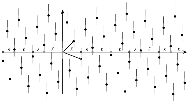
Figure 6: Equivalent description of the Fibonacci chain in terms of ‘targets’, often referred to as ‘occupation domains’ or ‘atomic surfaces’.

Familiar examples of model sets are some one-dimensional substitution-based structures such as the Fibonacci chain discussed above, and some of its generalisations. Planar examples include the Penrose tiling and the Tübingen triangle tiling with decagonal symmetry, the Ammann-Beenker tiling with octagonal symmetry and the shield tiling with dodecagonal symmetry, which can all be obtained by projection from four-dimensional lattices. Structure models of icosahedral quasicrystals usually employ model sets based on the (primitive, face-centred or body-centred) hypercubic lattice in six dimensions. These examples have direct application to the crystallography of quasicrystals, and serve as models for the structure of decagonal, octagonal, dodecagonal and icosahedral quasicrystals, respectively; compare Steurer & Deloudi (2009) for details. Realisations of model sets with other symmetries, such as planar sevenfold symmetry for instance, have as yet not been observed in nature, and the same is true for model sets where the internal space is not Euclidean. Nevertheless, such systems share many properties with the familiar quasicrystalline cases, and should not be excluded a priori. Even if it may prove impossible to realise such structures in self-assembled systems, we may be able to produce these in purpose-made manufactured structures at various length scales, from macroscopic to nanometre and atomic scales.

Arguably the most important result in the theory of model sets, in the context of mathematical diffraction theory, is the proof that regular model sets have pure point diffraction. Three different approaches have been used to prove this statement. The first proof using methods of dynamical systems theory was completed by Schlottmann (2000), employing an argument by Dworkin (1993) and the mathematical diffraction approach of Hof (1995); see also Lenz & Strungaru (2009) for further developments. An alternative approach employs the theory of almost periodic measures (Baake & Moody 2004, Moody & Strungaru 2004, Strungaru 2005). Following a suggestion by Lagarias, Baake & Grimm (2013) present a proof based on Poisson’s summation formula for the embedding lattice in conjunction with Weyl’s lemma on uniform distribution, which exploits the uniform distribution of projected lattice points in internal space. Although it has not been developed into a proof, there is also a somewhat complementary approach based on an average periodic structure; we refer to the recent review by Wolny, Kozakowski, Kuczera, Strzalka & Wnek, A. (2011) and references therein for details.

Essentially, the pure point diffraction of a model set is a consequence of the underlying higher-dimensional lattice periodicity. Let us first discuss the example of the Fibonacci model set $\varLambda$ of Eq. (8); compare also Figure 5. The pure point diffraction pattern is obtained again as a projection to physical space, but this time of the dual (or reciprocal) higher-dimensional lattice $\mathcal{L}^{*}$. In our case, this is the lattice generated by the dual basis vectors $\frac{2\tau-1}{5}(\tau-1,\tau)$ and $\frac{2\tau-1}{5}(1,-1)$. The corresponding Fourier module is then

$$L^{\circledast}\,=\,\pi(\mathcal{L}^{*})\,=\,\frac{1}{\sqrt{5}}\,\mathbb{Z}[\tau]\,,$$

where $\mathbb{Z}[\tau]=\{m+n\tau\mid m,n\in\mathbb{Z}\}$ as above. The determines the positions of Bragg peaks, but what about their intensities? It turns out that the intensity is a function of the distance of the projected lattice point from the physical space, and roughly the larger the internal coordinate the smaller the intensity. The function in question is the absolute square of the Fourier transform of the window function (the characteristic function of the window), which is the function that takes the value $1$ on the window and $0$ otherwise. Its Fourier transform is

$$A(k)\,=\,\mathrm{e}^{\pi\mathrm{i}k^{\star}(\tau-2)}\,\frac{\tau+2}{5}\,\mathrm{sinc}(\pi\tau k^{\star})\,,$$ (11)

where $\mathrm{sinc}(x)=\sin(x)/x$, and $k^{\star}$ is the image of $k$ under the $\star$-map introduced above. A sketch of the diffraction pattern is shown in Figure 7.

Figure 7: Sketch of the projection of the dual lattice points giving rise to Bragg peaks in the diffraction pattern for the Fibonacci point set $\varLambda$, with scatterers of unit weight at all points. The function displayed on the right-hand side is the intensity function $\lvert A(k)\rvert^{2}$. The Bragg peak at $0$ has height $(\mathrm{dens}(\varLambda))^{2}=(\tau+1)/5\approx 0.5206$, and the entire pattern (once all reflections are included) is reflection symmetric.

Let us now return to the general result. For a regular model set $\varLambda$ with Dirac comb $\delta_{\varLambda}$, the diffraction measure $\widehat{\gamma}$ can be written as

$$\widehat{\gamma}\,=\sum_{k\in L^{\circledast}}\lvert A(k)\rvert^{2}\,\delta_{k}\,,$$ (12)

where $L^{\circledast}=\pi(\mathcal{L}^{*})$, the projection of the higher-dimensional dual lattice, is the corresponding Fourier module on which the pure point diffraction is supported. For a Euclidean model set with the CPS (9), $\mathcal{L}$ is a lattice in a Euclidean space $\mathbb{R}^{d+m}$, and the Fourier module $L^{\circledast}$ is thus finitely generated, with rank $d+m$. By choosing appropriate generating vectors, the pure point diffraction of Eq. (12) can thus be recast in the form of Eq. (1) with $n=d+m$. However, in the general situation, where the internal space can be any locally compact Abelian group, this is not necessarily the case, as the Fourier module $L^{\circledast}=\pi(\mathcal{L}^{*})$ does not have to be finitely generated. Note that the latter case is not covered by the definition of a crystal cited above, while it does include any model set based on a Euclidean CPS.

The diffraction amplitudes $A(k)$ are obtained by the Fourier transform of the characteristic function $1_{W}$ of the window $W$,

$$A(k)\,=\,\frac{\mathrm{dens}(\varLambda)}{\mathrm{vol}(W)}\,\widehat{1_{W}}(-k^{\star})\,.$$ (13)

According to Eq. (12), it is the absolute square of these amplitudes that determine the intensity of a Bragg peak as position $k\in L^{\circledast}$, with $k^{\star}$ denoting the corresponding point in internal space. Eq. (13) gives the result for Euclidean model sets, the only difference for the general case is that the volume (with respect to Lebesgue measure in Euclidean space) is replaced by the suitable invariant measure (Haar measure) on the locally compact Abelian group.

5 Order beyond crystals

The current definition of crystals thus covers conventional periodic crystals, incommensurate crystals and quasicrystals, and hence all currently known realisations of perfectly ordered structures in nature. While the question asked by Bombieri & Taylor (1986) has not yet been satisfactorily answered, it is clear that pure point diffraction is a severe constraint on the possible structure (Baake, Lenz & Richard 1997), and recent results by Lenz & Moody (2009, 2011) indicate that model sets play a major role in a potential abstract parametrisation of the inverse problem. However, there are clearly well-ordered structures that do not possess this property, and this section will discuss a few characteristic examples. But first, we start with an example of a pure point diffractive system with non-finitely generated Fourier module, which thus possesses a diffraction pattern where Bragg peaks cannot be indexed by a finite number of integers.

5.1 Pure point diffraction with non-finitely generated support

Well-known examples of systems with non-Euclidean internal spaces are limit-periodic structures. Let us explain this with the arguably simplest example, based on the period doubling substitution rule $\varrho\!:1\mapsto 10,0\mapsto 11$, on the two-letter alphabet $\{0,1\}$. Any bi-infinite word $w\in\{0,1\}^{\mathbb{Z}}$ that satisfies the fixed point property $\varrho^{2}(w)=w$ is specified completely by $w(2n)=1$, $w(4n+1)=0$ and $w(4n+3)=w(n)$ for $n\in\mathbb{Z}$, while either letter can be chosen at position $n=-1$. The two possible choices lead to two locally indistinguishable sequences (which means that any finite subsequence of one occurs in the other), and hence define the same system.

The word $w$ possesses a Toeplitz structure consisting of a hierarchy of scaled and shifted copies of $\mathbb{Z}$ which carry the same letter. Defining the point set

$$\varLambda\,=\,\{n\in\mathbb{Z}\mid w(n)=1\}\subset\mathbb{Z}$$ (14)

of the positions of the letter $1$ in $w$, it is clear from the relations above that $2\mathbb{Z}\subset\varLambda$, as all letters at even positions are $1$. But then, due to $w(4n+3)=w(n)$, so are all letters $w(8n+3)=w(2n)=1$, so $8\mathbb{Z}+3\subset\varLambda$, and inductively one recognises that $2\cdot 4^{\ell}\mathbb{Z}+(4^{\ell}-1)\subset\varLambda$ for all integer $\ell\geq 0$. In fact, this hierarchy of scaled integer lattices describes the complete set, and we obtain the following representation for the set as a union (Baake, Moody & Schlottman 1998, Baake & Moody 2004, Baake & Grimm 2013)

$$\varLambda\,=\,2\,\mathbb{Z}\cup(8\,\mathbb{Z}+3)\cup(32\,\mathbb{Z}+15)\cup\dots\,=\,\bigcup_{\ell\geq 0}\bigl{(}(2\cdot 4^{\ell}\,\mathbb{Z}+(4^{\ell}-1)\bigr{)}$$ (15)

of scaled (and shifted) lattices. Note that this result is for the case where we choose $w(-1)=0$ (otherwise $-1$ has to be added to the right-hand side). A schematic representation of the corresponding Dirac comb $\delta_{\varLambda}$ is shown in Figure 8.

Figure 8: Schematic representation of the Dirac comb $\delta_{\varLambda}$ of the period doubling point set of Eq. (14). All point measures have the same mass. The different shading highlights the Toeplitz structure, with point masses at even integers shown in black, point masses on $8\mathbb{Z}+3$ in dark grey and a single point mass in $32\mathbb{Z}+15$ in lighter grey.

Figure 9: Schematic representation of the diffraction intensity pattern of the Dirac comb $\delta_{\varLambda}$ of Figure 8. The pattern is periodic with period $1$ and consists of a dense set of Bragg peaks, where increasingly smaller peaks are located at rational numbers whose denominators are increasingly larger powers of $2$. Note that only peaks corresponding to $r=0,1,2,3$ in Eqs. (16) and (17) are visible here.

Using this representation for the point set $\varLambda$, the diffraction of the Dirac comb $\delta_{\varLambda}$ can be computed explicitly; see Baake & Grimm (2011b) for details. The scaled lattices with geometrically increasing period in the union in Eq. (15) give rise to Bragg peaks supported on the corresponding dual lattices, which are successively finer integer lattices scaled with the inverse factor. The diffraction spectrum is pure point, and the Fourier module can be parametrised as

$$L^{\circledast}\,=\,\mathbb{Z}[\tfrac{1}{2}]\,=\,\bigl{\{}\tfrac{m}{2^{r}}\mid(r=0,m\in\mathbb{Z})\text{ or }(r\geq 1,m\text{ odd})\bigr{\}}\,.$$ (16)

The diffraction measure is of the form of Eq. (12), with diffraction amplitudes

$$A\bigl{(}\tfrac{m}{2^{r}}\bigr{)}\,=\,\frac{2}{3}\,\frac{(-1)^{r}}{2^{r}}\,\mathrm{e}^{2^{1-r}\pi\mathrm{i}m}$$ (17)

at the positions in $L^{\circledast}$. The factor of $\frac{2}{3}$ reflects the density of scatterers, as two thirds of positions are occupied. It is no coincidence that the model set expression applies — in fact, the set $\varLambda$ can be described as a model set, but with a non-Euclidean internal space; in this case, the internal space is what is known as the space of $2$-adic integers (which essentially consists of all fractions whose denominators are powers of $2$, but with a specific definition of the distance of two numbers). A schematic representation of the diffraction pattern for the period doubling chain is shown in Figure 9.

It is easy to generalise this example to other lattice-based substitutions in one or more dimensions; any substitution of constant length $p$ with a coincidence in the sense of Dekking (1978), which means that the same letter appears at the same position for the images of all letters under a certain power of the substitution rule, is a good candidate, because it is always pure point diffractive and carries a natural $p$-adic structure. A well-known example of this type is the chair tiling, in its representation as a two-dimensional block substitution; see Robinson (1999) and Baake & Grimm (2013) for details.

5.2 Order and singular continuous diffraction

The paradigm of singular continuous diffraction is provided by the Thue–Morse system and its generalisations (Kakutani 1972, Baake & Grimm 2008). Here, we consider a family of generalised Thue–Morse substitutions (Baake, Gähler & Grimm 2012)

$$\varrho^{(k,\ell)}:\;\begin{array}[]{r@{\;}c@{\;}l}1&\mapsto&1^{k}\,\bar{1}^{\ell}\\ \bar{1}&\mapsto&\bar{1}^{k}\,1^{\ell}\end{array}$$ (18)

on the two-letter alphabet $\{1,\bar{1}\}$, where $k,\ell\in\mathbb{N}$ and the case $k=\ell=1$ corresponds to the classic Thue–Morse case. Note that $1^{j}$ denotes a string of $j$ consecutive letters $1$ here. The one-sided fixed point $v=\varrho^{(k,\ell)}(v)$ satisfies

$$v_{(k+\ell)m+r}\,=\,\begin{cases}v_{m},&\text{if $0\leq r\leq k-1$},\\ \bar{v}_{m},&\text{if $k\leq r\leq k+\ell-1$}\end{cases}$$ (19)

where $m\geq 0$ and $0\leq r\leq k+\ell-1$ and $\bar{\bar{1}}=1$. It extends (by setting $v_{-i-1}=v_{i}$ for $i\geq 0$) to a symmetric bi-infinite fixed point word under the square of the substitution $\varrho^{(k,\ell)}$. For instance, the symmetric bi-infinite fixed point for the classic Thue–Morse case $k=\ell=1$ has core

$$\ldots\bar{1}11\bar{1}1\bar{1}\bar{1}1\bar{1}11\bar{1}\bar{1}11\bar{1}1\bar{1}\bar{1}1\big{|}1\bar{1}\bar{1}1\bar{1}11\bar{1}\bar{1}11\bar{1}1\bar{1}\bar{1}1\bar{1}11\bar{1}\ldots$$

where the vertical bar denotes the origin. A schematic representation of the corresponding Dirac comb is shown in Figure 10.

Figure 10: Schematic representation of the Dirac comb of the Thue–Morse chain with weights $\pm 1$. Note that this is ‘balanced’ in the sense that positive and negative weights are equally frequent, so the average scattering strength is zero.

The corresponding weighted Dirac comb on $\mathbb{Z}$, interpreting the two letters as weights (with $\bar{1}$ interpreted as $-1$), is thus given by $\omega=\sum_{i\in\mathbb{Z}}v_{i}\delta_{i}$. Its autocorrelation $\gamma=\sum_{m\in\mathbb{Z}}\eta(m)\delta_{m}$ is also a Dirac comb on $\mathbb{Z}$, where the autocorrelation coefficients $\eta(m)$ satisfy $\eta(0)=1$, $\eta(-m)=\eta(m)$ and the recursion relation

$$\begin{split}\eta\bigl{(}(k+\ell)m+r\bigr{)}\,=\,\frac{1}{k+\ell}\Bigl{(}&\alpha(k,\ell,r)\,\eta(m)+\\ &\alpha(k,\ell,k+\ell-r)\,\eta(m+1)\Bigr{)}\end{split}$$ (20)

for arbitrary $m\in\mathbb{Z}$ and $0\leq r\leq k+\ell-1$. The recursion follows directly from Eq. (19), with $\alpha(k,\ell,r)=k+\ell-r-2\min(k,\ell,r,k+\ell-r)$. This system has a unique solution, and properties of the solution show that the corresponding diffraction measure $\widehat{\gamma}$ is purely singular continuous; see Baake, Gähler & Grimm (2012) for the mathematical details of the argument.

       

       

Figure 11: Approximating density functions $f^{(N)}$ (top) and corresponding approximating distribution function $F^{(N)}$ (bottom) for the diffraction of the classic Thue–Morse chain ($k=\ell=1$) with $N=4$ (left), $N=5$ (centre) and $N=6$ (right).

The diffraction measure is periodic with period $1$ (due to the fact that the Dirac comb is supported on the integer lattice $\mathbb{Z}$) and the diffraction intensity can be represented as a limit of a product,

$$f^{(N)}(x)\,=\prod_{n=0}^{N}\vartheta\bigl{(}(k+\ell)^{n}x\bigr{)}\,,$$

which is known as a Riesz product, with

$$\vartheta(x)\,=\,1+\frac{2}{k+\ell}\!\sum_{r=1}^{k+\ell-1}\!\!\alpha(k,\ell,r)\,\cos(2\pi rx).$$

The limit as $N\to\infty$ has to be considered carefully. While the truncated product $f^{(N)}$ is a smooth function that can be interpreted as a density of an absolutely continuous measure, this is not the case in the limit, because it represents a purely singular continuous measure. Accordingly, the approximating density functions $f^{(N)}$ become increasingly spiky with growing value of $N$; see Figure 11 for an example. Mathematically, we speak of a limit in the vague topology. However, the corresponding distribution function $F^{(N)}(x)=\int_{0}^{x}f^{(N)}(x)\,\mathrm{d}x$ (which corresponds to the integrated diffraction intensity) converges and possesses a continuous limit; compare the bottom part of Figure 11. The limit function can be calculated and expressed as an explicit Fourier series; several examples are shown in Figure 12.

       

Figure 12: Continuous distribution functions for the diffraction of generalised Thue–Morse chains with $\ell=1$ and $k=2$ (left), $k=3$ (centre) and $k=4$ (right).

While this case has no point spectrum (the trivial Bragg peak at $0$ being absent due to our balanced choice of weights, corresponding to zero average scattering strength), it is by no means featureless. In fact, there are peaks that grow with certain scaling exponents (in terms of the system size) at certain points in Fourier space (the most prominent examples can be found at rational positions $\frac{1}{3}$ and $\frac{2}{3}$ in Figure 11), while the growth is not well defined at uncountably many other positions (due to the non-convergence of the density functions); see Baake, Grimm & Nilsson (2014) for a detailed account of the classic Thue–Morse case.

Clearly, the generalised Thue–Morse systems possess hierarchical order, although this is not reflected in a pure point component in their diffraction measures. However, this ‘hidden’ order is visible in other correlations. Explicitly, it can be revealed by looking at the two-point correlations of pairs rather than of single points. Looking at pairs can be described by considering the image of the bi-infinite fixed point word $v$ under a sliding block map $\phi$, which maps pairs of adjacent letters to $a$ or $b$ according to whether they are equal or different, so $\phi\!:\,11,\bar{1}\bar{1}\mapsto a,\;1\bar{1},\bar{1}1\mapsto b$; see Figure 13 for an illustration.

Figure 13: The action of the sliding block map $\phi$ on a Thue–Morse word produces a period doubling word.

This maps the set of generalised Thue–Morse words to bi-infinite words which are locally indistinguishable to fixed point words of the generalised period doubling substitution

$$a\mapsto b^{k-1}ab^{\ell-1}b,\quad b\mapsto b^{k-1}ab^{\ell-1}a,$$

which reduces to the period doubling substitution (with $a=1$ and $b=0$) in the case $k=\ell=1$. This map is globally $2:1$, meaning that there are precisely two generalised Thue–Morse words that are mapped onto the same generalised period doubling word. This is most easily seen by noticing that, when going backwards from a generalised period doubling word, there is a single free choice for one letter $a$ or $b$ at one position, where either preimage can be chosen, after which all other preimages are uniquely determined (due to the overlap of adjacent pairs). As the generalised period doubling substitution has a coincidence in the sense of Dekking (1978), it is pure point diffractive, as discussed above for the (standard) period doubling case. In fact, the corresponding point sets are model sets, this time with $(k+\ell)$-adic numbers as internal space, and the pure point diffraction is supported on the set $\mathbb{Z}[\frac{1}{k+\ell}]$, which contains all inverse powers of $(k+\ell)$ as generating elements.

In the language of dynamical systems, the dynamical system (where the dynamics is given by shifting the sequence by an integer) corresponding to generalised period doubling words constitutes a factor of the dynamical system associated to the generalised Thue–Morse words. Here, the word factor refers to the fact that it is the image under the sliding block map $\phi$. What happens in this case is that the diffraction spectrum of the factor (the generalised period doubling system) picks up a non-trivial point spectrum, which is ‘hidden’ in the Thue–Morse system, in the sense that it does not show up in its diffraction spectrum (even in the case of general weights). However, this pure point spectrum is part of the so-called dynamical spectrum of the Thue–Morse system, where the dynamical spectrum refers to the spectrum of the operator which generates the translation action; see Queffélec (2010) for details. The dynamical spectrum is, in general, richer than the diffraction spectrum. This can be intuitively understood because diffraction, as the Fourier transform of the autocorrelation, only measures two-point correlations, while the dynamical spectrum ‘knows’ about more general properties under the shift action, so effectively can probe higher correlations. We shall come back to this point at the end of this section.

5.3 Order and absolutely continuous diffraction

Absolutely continuous (‘diffuse’) diffraction is commonly associated with randomness. Indeed, stochastic systems typically show absolutely continuous diffraction; the simplest case is the Bernoulli shift, based on a random sequence

$$X\,=\,(\ldots,X_{-2},X_{-1},X_{0},X_{1},X_{2},\ldots)\,\in\,\{\pm 1\}^{\mathbb{Z}}$$

of independent and identically distributed (i.i.d.) events with outcome $\pm 1$, with probability $p$ for outcome $1$ and probability $1-p$ for outcome $-1$. The Bernoulli shift has (metric) entropy $H(p)=-p\log(p)-(1\!-\!p)\log(1\!-\!p)$, which is greater than zero except for the deterministic limiting cases $p=0$ and $p=1$. All the examples discussed earlier were deterministic sequences with zero entropy.

A random sequence $X\in\{\pm 1\}^{\mathbb{Z}}$ leads to a Dirac comb $\omega=\sum_{j\in\mathbb{Z}}X_{j}\delta_{j}$, which is a translation bounded random measure with autocorrelation $\gamma_{\mathrm{B}}=\sum_{m\in\mathbb{Z}}\eta_{\mathrm{B}}(m)\,\delta_{m}$. The autocorrelation coefficients are, almost surely (in the probabilistic sense, so with probability $1$), given by

$$\begin{split}\eta_{\mathrm{B}}(m)\,=\,\begin{cases}1,&m=0,\\ (2p\!-\!1)^{2},&m\neq 0.\end{cases}\end{split}$$

as a consequence of the strong law of large numbers. The corresponding diffraction measure then, almost surely, is given by

$$\widehat{\gamma_{\mathrm{B}}}\,=\,(2p-1)^{2}\delta_{\mathbb{Z}}\,+\,4p(1-p)\,\lambda\,,$$

which contains both pure point (for $p\neq\frac{1}{2}$) and absolutely continuous components (for $p\not\in\{0,1\}$). The pure point part vanishes when both weights appear with equal probability, while the absolutely continuous part vanishes in the two deterministic, periodic cases.

Figure 14: Schematic representation of the Dirac comb of the Rudin–Shapiro chain with weights $\pm 1$, which is again ‘balanced’ in the sense that the average scattering strength is zero.

It is, however, possible to construct deterministic systems with absolutely continuous diffraction as well. The paradigm for this situation is the Rudin–Shapiro chain (Rudin 1959, Shapiro 1951, Queffélec 2010). Its binary version $w\in\{\pm 1\}^{\mathbb{Z}}$ can be defined by initial conditions $w(-1)=-1$, $w(0)=1$, and the recursion

$$w(4n+\ell)=\begin{cases}w(n),&\mbox{for $\,\ell\in\{0,1\}$,}\\ (-1)^{n+\ell}\,w(n),&\mbox{for $\,\ell\in\{2,3\}$.}\end{cases}$$ (21)

A schematic representation of the corresponding Dirac comb is shown in Figure 14. By considering the recursion relation for autocorrelation coefficients induced by Eq. (21), in a similar way as for the generalised Thue–Morse case above, on can show (Baake & Grimm 2009) that the autocorrelation has the simple form $\gamma_{\mathrm{RS}}=\delta_{0}$, which means that all correlations (apart from the trivial case with distance zero) average to zero along the chain. According to the two-point correlations, the Rudin–Shapiro chain hence looks completely uncorrelated, exactly as the random chain with probability $p=\frac{1}{2}$. As a consequence, the diffraction measure is Lebesgue measure, $\widehat{\gamma_{\mathrm{RS}}}=\lambda$, which is clearly absolutely continuous with respect to itself. This means that the diffraction intensity is constant in space, and hence completely featureless, reflecting the complete absence of two-point correlation in the structure. This example shows that two very different systems such as the $p=\frac{1}{2}$ Bernoulli chain with entropy $\log(2)$ and the completely deterministic binary Rudin–Shapiro chain (with zero entropy) can produce the same autocorrelation and hence the same diffraction measure. Such structures are called homometric (Patterson 1944) and show that the inverse problem does not have a unique solution in general.

In fact, the situation is worse than that, as from the results above one can construct an entire one-parameter family of stochastic Dirac combs which all are homometric with the Rudin–Shapiro chain. This is done by the Bernoullisation procedure (Baake & Grimm 2009). Applying it to the Rudin–Shapiro Dirac comb, the weight at any position is changed randomly with probability $1-p$, resulting in

$$\omega\,=\,\sum_{j\in\mathbb{Z}}w_{j}\,X_{j}\,\delta_{j}\,,$$

with the Rudin–Shapiro sequence $w\in\{\pm 1\}^{\mathbb{Z}}$ and the random sequence $X\in\{\pm 1\}^{\mathbb{Z}}$ as defined above. This is a ‘model of second thoughts’ in the sense that, when starting from a Rudin–Shapiro sequence, weights are randomly changed with probability $1-p$ independently at each position along the chain. We thus can continuously interpolate between the Rudin–Shapiro chain with entropy $0$ and the $p=\frac{1}{2}$ Bernoulli chain with entropy $\log(2)$, with all systems sharing the same absolutely continuous diffraction.

It is interesting to note that the Rudin–Shapiro chain, like the generalised Thue–Morse chains above, possesses a ‘hidden’ limit-periodic order that is revealed when looking at an appropriate dynamical factor. Using the same sliding block map $\phi$ as above, one obtains once more a factor with pure point diffraction spectrum, in this case supported on $\mathbb{Z}[\frac{1}{2}]$, as for the period doubling case; see Baake & Grimm (2013) for details. Clearly, this does not happen for the stochastic chain, which does not have any ‘hidden’ order.

5.4 Discrete structures with continuous symmetry

An interesting (and still somewhat mysterious) class of structures is provided by discrete systems which possess a continuous symmetry. The paradigm for such a structure is the Conway–Radin pinwheel tiling (Radin 1994). It is an inflation tiling based on a single triangular prototile of edge lengths $1$, $2$ and $\sqrt{5}$ together with its reflected version. The inflation rule is shown in Figure 15; it consists of a linear rescaling by the inflation factor $\sqrt{5}$ (first step) and the dissection of the inflated triangle into five copies of the original prototile (second step), where both orientations occur. The reflected rule applies to the reflected triangle, and hence the tiling is reflection symmetric. A realisation of the tiling is shown in Figure 16.

Figure 15: Inflation rule for the pinwheel tiling. The dot marks the reference point, and the shading emphasises that the particular triangle is in the original position and orientation, ensuring that repeated application of the inflation rule produces a fixed point tiling.

Figure 16: A building at Melbourne’s Federation Square featuring a pinwheel tiling façade.

What makes this inflation rule special is the rotation it introduces between copies of the prototiles. This rotation by an angle $\vartheta=-\arctan(\frac{1}{2})$ is incommensurate with $\pi$, and as a result introduces new, independent directions under inflation. Iteration of the inflation rule on an initial patch thus leads to patches comprising an exponentially increasing number of triangles occurring in a linearly growing number of independent directions. In the limit of an infinite tiling, triangles appear in infinitely many different orientations. While for the familiar cases of Penrose-type tilings inflation rules produce tilings with discrete (in the Penrose case decagonal) symmetry (in the sense that the tiling space defined by the fixed point tilings has decagonal symmetry; see Baake & Grimm (2013) for details), the pinwheel inflation produces a tiling space with complete circular symmetry (Radin 1994, Radin 1997, Moody, Postnikoff & Strungaru 2006). As a consequence, its diffraction is circularly symmetric as well, and hence cannot have any pure point component apart from the trivial Bragg peak at the origin.

In fact, the rotation is rather special, because it is a coincidence rotation for the planar square lattice, as $\tan(\vartheta)=-\frac{1}{2}$ is rational; see Baake (1997) for background. This property is behind the observation that the point set of pinwheel reference points can either be seen as a subset of rotated square lattices or a subset of scaled square lattices, with scaling by inverse powers of $5$ (Baake, Frettlöh & Grimm 2007a), which makes it possible to draw conclusions on the diffraction spectrum by using a radial version of Poisson’s summation formula. This provides evidence that the diffraction consists of sharp rings, and that it is surprisingly similar to a toy model of powder diffraction of square lattice structures (Baake, Frettlöh & Grimm 2007a, 2007b). A diffraction measure supported on sharp rings in the plane is singular continuous, and it is clear that the diffraction of the pinwheel tiling contains singular continuous components of this type; however, to date there is no complete characterisation of the diffraction spectrum of this example. Results of numerical investigations suggest that an absolutely continuous component may also be present. An approximation of the radially averaged diffraction is shown in Figure 17.

Figure 17: Approximation of radial diffraction intensity $I(k)$ for the pinwheel diffraction (black line), based on data from a finite system. The grey columns indicate the sharp rings observed in a toy model of powder diffraction from a planar square-lattice structure, with the relative scale adjusted according to the first main peak; see Baake, Frettlöh & Grimm (2007a, 2007b) for details.

While the pinwheel tiling may seem a rather exotic structure, it is generated by a quite simple inflation rule with only a single shape up to congruency. There are many other structures of this type; see Frettlöh (2008) for some examples.

5.5 Diffraction versus dynamical spectra

The examples of the Thue–Morse and Rudin–Shapiro systems show that systems can possess ‘hidden’ order that does not manifest itself by a pure point component in the diffraction pattern. However, this order can show up in the dynamical spectrum, which is related to the analysis of the translation action on the structure. There is a close relationship between these two spectral quantities — indeed, the first proofs of the pure point diffractivity of model sets employed the link to dynamical spectra, using the results that the diffraction spectrum is pure point if and only if the dynamical spectrum is. In general, however, the dynamical spectrum can be richer (van Enter & Miȩkisz 1992), and the Thue–Morse and Rudin–Shapiro systems are examples; in both cases, the dynamical spectrum contains the pure point component $\mathbb{Z}[\frac{1}{2}]$ which arises because both examples stem from primitive substitutions of constant length $2$ (in the Rudin–Shapiro case, the underlying substitution employs four different letters, and the binary system is derived from this by identifying pairs of letters; see Baake & Grimm (2013) for details).

A particularly simple yet striking example, originally suggested by van Enter, is discussed in Baake & van Enter (2011). It considers the set of certain configurations of $\pm 1$ on the integer lattice $\mathbb{Z}$. The allowed configurations $w\in\{\pm 1\}^{\mathbb{Z}}$ are obtained by partitioning the lattice into pairs of neighbouring points (there are two ways to do this), and then randomly assigning to each pair either the values $(+1,-1)$ or $(-1,+1)$. Turning a configuration $w$ into a signed Dirac comb with weights $w_{i}\in\{\pm 1\}$, it is easy to show, by an application of the strong law of large numbers, that the autocorrelation is (almost surely) given by $\gamma=\delta_{0}-\frac{1}{2}(\delta_{1}+\delta_{-1})$. The corresponding diffraction measure is then

$$\widehat{\gamma}\,=\,\bigl{(}1-\cos(2\pi k)\bigr{)}\lambda\,,$$

and hence purely absolutely continuous, where the Radon-Nikodym density relative to $\lambda$ is written as a function of $k$. However, the dynamical spectrum of this system contains eigenvalues (hence a pure point part), reflecting the order in the system imposed by the ‘dimer’ condition on pairs. This can be revealed by considering a block map similar to to the map $\phi$ used above. Explicitly, setting $u_{i}=-w_{i}w_{i+1}$ for $i\in\mathbb{Z}$ maps $w$ to a new sequence $u$, which (almost surely) has the diffraction measure

$$\widehat{\gamma_{u}}\,=\,\tfrac{1}{4}\,\delta_{\mathbb{Z}/2}+\tfrac{1}{2}\,\lambda\,;$$

see Baake & van Enter (2011) for details. The ‘dimer’ structure is reflected in the presence of the pure point part supported on $\frac{1}{2}\mathbb{Z}$, which also is the entire point part of the dynamical spectrum.

This example again shows that the ‘hidden’ order can also be seen in diffraction, but not in the original system. Note that simply changing the weights of the scatterers will not achieve this, although it may contribute a trivial Bragg part. However, choosing a suitable factor (or a family of factors) as an image of a continuous map such as the sliding block map $\phi$ used above, makes it possible to detect the ‘hidden’ order via its diffraction. That this is a general property of the relation between dynamical and diffraction spectrum is a recent non-trivial insight; see Baake, Lenz & van Enter (2013) for the latest developments in this direction.

6 Conclusions

The discoveries of incommensurately modulated and aperiodically ordered solids in the twentieth century (de Wolff 1974, Janner & Janssen 1977, Shechtman, Blech, Gratias & Cahn 1984, Ishimasa, Nissen & Fukano 1985) have changed our view of crystallography. Crystallography is no longer restricted to the analysis of lattice periodic arrangements of atoms or molecules, but takes a broader view which includes certain aperiodically ordered structures, such as incommensurate crystals and quasicrystals. The definition of a crystal has been amended to reflect this broader view.

The definition of a crystal is based on the currently known catalogue of periodic and aperiodic crystals. We presently do not know of any materials that have aperiodically ordered structures beyond incommensurate crystals (including composite structures) and quasicrystals. For the latter, so far only symmetries corresponding to the smallest embedding dimension (in the sense of model sets) have been observed, with octogonal, decagonal and dodecagonal quasicrystal planes corresponding to projections from four-dimensional periodic structures, and icosahedral quasicrystals being described by projection from six-dimensional lattices. However, there is no a priori reason that excludes other symmetries completely, or indeed aperiodically ordered structures that are not described by model sets obtained from projections of a lattice in a finite-dimensional Euclidean space.

The definition of a crystal also reflects the current lack of understanding of what constitutes order in matter (and more generally), and in this sense should be seen as a working definition that may well need to be revised in the future. In crystallography, order is linked to diffraction, which makes sense because diffraction is the method of choice to experimentally determine the structure of a solid. The examples discussed above demonstrate that there are ordered structures which are not captured by the current definition, either because their pure point diffraction fails to be finitely generated, or because they do not have any non-trivial point component in their diffraction. While we do not know whether such structures are realised in nature, it should become possible to manufacture such materials with purpose-designed structures and properties. In this sense, these structures are relevant and should be considered to be within the realm of crystallography.

From a mathematical point of view, a more satisfying attempt at defining order might employ the dynamical spectrum, which is a generalisation of the diffraction spectrum. The results above are in line with the intuition by van Enter & Miȩkisz (1992) that an apparent disorder at an ‘atomic’ scale could be accompanied by order at a ‘molecular’ scale, with diffraction of derived factor structures probing the latter. While diffraction itself only measures the averaged two-point correlations in a structure, the dynamical spectrum probes the repetitivity of a structure under translations, and hence also higher-order correlations, which generally can distinguish homometric systems (Grünbaum & Moore 1995). While these are not necessarily directly accessible by experiment, the additional information contained in the dynamical spectrum is, in principle, encoded in diffraction spectra of derived systems; see Baake, Lenz & van Enter (2013) for recent developments on establishing this connection. Defining order via a non-trivial pure point component of the dynamical spectrum would include structures such as the Thue–Morse and Rudin–Shapiro systems, though presumably examples of pinwheel type (for which the dynamical spectrum is not known) would be excluded. In this sense, it probably is still not completely satisfactory to capture all possible manifestations of order, but it may provide a first step towards a better understanding.

In this paper, the discussion was limited to deterministic systems, apart from the brief excursion on the Bernoulli chain. Clearly, moving to partially ordered systems, which contain an element of stochastic disorder, is relevant as well. Not only does even the most perfect crystal contain some amount of disorder, but there are also entropically stabilised structures with intrinsic configurational disorder, among them many quasicrystalline phases. In this context, the notion of ‘entropic order’ is relevant, which has been investigated in statistical physics, in particular with respect to the physics of glasses; see, for instance, Kurchan & Levine (2011), Sasa (2012a, 2012b) and Wolff & Levine (2014) for recent work along these lines.

Although the importance of random tiling structures was pointed out early on (Elser 1985), and while there is some good heuristic information from scaling considerations (Henley 1999), there are as yet very few mathematically rigorous results for non-trivial random tiling structures in two or more dimensions, the only examples known being related to solvable models of lattice statistical mechanics (Baake & Höffe 2000). We refer to Baake, Birkner & Grimm (2015) for a recent review on what is known about the diffraction of partially ordered and stochastic systems.

References

Authier, A. (2013). Early Days of X-ray Crystallography, Oxford: Oxford University Press.

Authier, A. & Chapuis, G. (2014). A Little Dictionary of Crystallography, International Union of Crystallography.

Baake, M. (1997). Solution of the coincidence problem in dimensions $d\leq 4$, in: The Mathematics of Long-Range Aperiodic Order, edited by R.V. Moody, pp. 9–44, Kluwer: Dordrecht.

Baake, M., Birkner, M. & Grimm U. (2015). Non-periodic systems with continuous diffraction measures, in: Mathematics of Aperiodic Order, edited by J. Kellendonk, D. Lenz & J. Savinien, in press, Boston: Birkhäuser.

Baake, M., Frettlöh, D. & Grimm, U. (2007a). A radial analogue of Poisson’s summation formula with applications to powder diffraction and pinwheel patterns. J. Geom. Phys. 57, 1331–1343. arXiv:math.SP/0610408.

Baake, M., Frettlöh, D. & Grimm, U. (2007b). Pinwheel patterns and powder diffraction, Philos. Mag. 87, 2831–2838. arXiv:math-ph/0610012.

Baake M., Gähler F. & Grimm U. (2012). Spectral and topological properties of a family of generalised Thue-Morse sequences, J. Math. Phys. 53, 032701. arXiv:1201.1423.

Baake, M., Gähler, F. & Grimm, U. (2013). Examples of substitution systems and their factors. J. Int. Seq. 16, article 13.2.14: 1–18. arXiv:1211.5466.

Baake, M. & Grimm, U. (2007). Homometric model sets and window covariograms. Z. Krist. 222, 54–58. arXiv:math.MG/0610411.

Baake, M. & Grimm, U.(2008). The singular continuous diffraction measure of the Thue-Morse chain. J. Phys. A: Math. Theor. 41, 422001: 1–6. arXiv:0809.0580.

Baake, M. & Grimm, U. (2009). Kinematic diffraction is insufficient to distinguish order from disorder. Phys. Rev. B 79, 020203(R): 1–4 and Phys. Rev. B 80, 029903(E). arXiv:0810.5750.

Baake, M. & Grimm, U. (2011a). Kinematic diffraction from a mathematical viewpoint. Z. Krist. 226, 711–725. arXiv:1105.0095.

Baake, M. & Grimm, U. (2011b). Diffraction of limit periodic point sets, Philos. Mag. 91, 2661–2670. arXiv:1007.0707.

Baake, M. & Grimm, U. (2012). Mathematical diffraction of aperiodic structures. Chem. Soc. Rev. 41, 6821–6843. arXiv:1205.3633.

Baake, M. & Grimm, U. (2013). Aperiodic Order. Vol. 1: A Mathematical Invitation. Cambridge: Cambridge University Press.

Baake, M. & Grimm, U. (2014). Squirals and beyond: Substitution tilings with singular continuous spectrum. Ergodic Theory and Dynamical Systems 34, 1077–1102. arXiv:1205.1384.

Baake, M., Grimm, U. & Nilsson, J. (2014). Scaling of the Thue-Morse diffraction measure, Acta Phys. Pol. A 126, 431–434. arXiv:1311.4371

Baake, M. & Höffe, M. (2000). Diffraction of random tilings: some rigorous results, J. Stat. Phys. 99, 219–261. arXiv:math-ph/9904005.

Baake, M., Lenz, D. & Richard, C. (1997). Pure point diffraction implies zero entropy for Delone sets with uniform cluster frequencies, Lett. Math. Phys. 82, 61–77. arXiv:0706.1677.

Baake, M., Lenz, D. & van Enter, A.C.D. (2013). Dynamical versus diffraction spectrum for structures with finite local complexity, Preprint arXiv:1307.5718.

Baake, M. & Moody, R.V. (2004). Weighted Dirac combs with pure point diffraction, J. reine angew. Math. (Crelle) 573, 61–94. arXiv:math.MG/0203030.

Baake, M., Moody, R.V. & Schlottmann, M. (1998). Limit-(quasi)periodic point sets as quasicrystals with $p$-adic internal spaces, J. Phys. A: Math. Gen. 31, 5755–5765. arXiv:math-ph/9901008.

Baake, M. & van Enter, A.C.D. (2011). Close-packed dimers on the line: diffraction versus dynamical spectrum, J. Stat. Phys. 143, 88–101. arXiv:1011.1628.

Bohr, H. (1947). Almost Periodic Functions, reprint, Chelsea: New York.

Bombieri, E. & Taylor, J.E. (1986). Which distributions of matter diffract? An initial investigation. J. Phys. Colloques 47, C3-19–C3-28.

Bragg, W.H. & Bragg, W.L. (1913). The reflection of X-rays by crystals. Proc. Roy. Soc. A 88, 428–438.

Córdoba, A. (1989). Dirac combs, Lett. Math. Phys. 17, 191–196.

Cowley, J.M. (1995). Diffraction Physics, 3rd edition, North-Holland: Amsterdam.

Dekking, F.M. (1978). The spectrum of dynamical systems arising from substitutions of constant length, Z. Wahrscheinlichkeitsth. verw. Geb. 41, 221–239.

de Bruijn. N.G. (1986). Quasicrystals and their Fourier transforms. Indag. Math. (Proc.) 89, 123–152.

de Wolff, P.M. (1974). The pseudo-symmetry of modulated crystal structures, Acta Cryst. A 30, 777–785.

Dworkin, S. (1993). Spectral theory and x-ray diffraction, J. Math. Phys. 34, 2965–2967.

Elser, V. (1985). Comment on “Quasicrystals: A new class of ordered structures”, Phys. Rev. Lett. 54, 1730.

Frettlöh, D. (2008). Substitution tilings with statistical circular symmetry, Europ. J. Combin. 29, 1881–1893. arXiv:0704.2521.

Friedrich, W., Knipping, P. & von Laue, M. (1912). Interferenz-Erscheinungen bei Röntgenstrahlen. Sitzungsberichte der Kgl. Bayer. Akad. der Wiss., 303–322.

Grünbaum, F.A. & Moore, C.C. (1995). The use of higher-order invariants in the determination of generalized Patterson cyclotomic sets, Acta Cryst. A 51, 310–323.

Henley, C.L. (1999). Random tiling models, in: Quasicrystals: The State of the Art, edited by D. P. DiVincenzo & P. J. Steinhardt, 2nd edition, pp 459–560, World Scientific: Singapore.

Hof, A. (1995) On diffraction by aperiodic structures, Commun. Math. Phys. 169, 25–43.

International Union of Crystallography (1992). Report of the Executive Committee for 1991. Acta Cryst. A 48, 922–946.

Ishimasa, T., Nissen H.-U. & Fukano, Y. (1985). New ordered state between crystalline and amorphous in Ni-Cr particles, Phys. Rev. Lett. 55, 511–513.

Janner, A. & and Janssen, T. (1977). Symmetry of periodically distorted crystals, Phys. Rev. B 15, 643–658.

Janssen, T. & Janner, A. (2014). Aperiodic crystals and superspace concepts. Acta Cryst. B 70, 617–651.

Kakutani, S. (1972). Strictly ergodic symbolic dynamical systems, in: Proc. 6th Berkeley Symposium on Math. Statistics and Probability, edited by L. M. LeCam, J. Neyman & E. L. Scott, pp. 319–326. Berkeley: University of California Press.

Kurchan, J. & Levine D. (2011). Order in glassy systems, J. Phys. A: Math. Theor. 44, 035001.

Lenz, D. & Moody, R.V. (2009). Extinctions and correlations for uniformly discrete point processes with pure point dynamical spectra, Commun. Math. Phys. 289, 907–923. arXiv:0902.0567.

Lenz, D. & Moody, R.V. (2011). Stationary processes with pure point diffraction. Preprint arXiv:1111.3617.

Lenz, D. & Strungaru, N. (2009). Pure point spectrum for measure dynamical systems on locally compact Abelian groups, J. Math. Pures Appl. 92, 323–341. arXiv:0704.2498.

Lifshitz, R. (2003). Quasicrystals: A matter of definition, Foundatiions of Physics 33, 1703–1711.

Lifshitz, R. (2007). What is a crystal? Z. Kristallogr. 222, 313–317.

Lifshitz, R. (2011). Symmetry breaking and order in the age of quasicrystals, Isr. J. Chem. 51, 1156–1167.

Meyer, Y. (1972). Algebraic Numbers and Harmonic Analysis, North Holland: Amsterdam.

Moody, R.V. (2000). Model sets: A survey, in: From Quasicrystals to More Complex Systems, edited by F. Axel, F. Dénoyer & J. P. Gazeau, pp. 145–166, EDP Sciences: Les Ulis, and Springer: Berlin. arXiv:math.MG/0002020.

Moody, R.V., Postnikoff D. & Strungaru N. (2006). Circular symmetry of pinwheel diffraction, Ann. Henri Poincaré 7, 711–730.

Moody, R.V. & Strungaru, N. (2004). Point sets and dynamical systems in the autocorrelation topology, Canad. Math. Bull. 47, 82–99.

Mumford, D. & Desolneux, A. (2010). Pattern Theory: The Stochastic Analysis of Real-World Signals, A K Peters: Natick, MA.

Patterson, A.L. (1944). Ambiguities in the X-ray analysis of crystal structures. Phys. Rev. 65, 195–201.

Queffélec, M. (2010). Substitution Dynamical Systems — Spectral Analysis, LNM 1294, 2nd edition, Springer: Berlin.

Radin, C. (1994). The pinwheel tilings of the plane, Ann. Math. 139, 661–702.

Radin, C. (1997). Aperiodic tilings, ergodic theory and rotations, in: The Mathematics of Long-Range Aperiodic Order, edited by R.V. Moody, pp. 499–519, Kluwer: Dordrecht.

Reed, M. & Simon, B. (1980). Methods of Modern Mathematical Physics I: Functional Analysis, 2nd edition, Academic Press: San Diego.

Robinson, E.A. (1999). On the table and the chair, Indag. Math. 10, 581–599.

Rudin, W. (1959). Some theorems on Fourier coefficients, Proc. Amer. Math. Soc. 10, 855–859.

Sasa S. (2012a). Statistical mechanics of glass transition in lattice molecule models, J. Phys. A: Math. Theor. 45, 035002.

Sasa S. (2012b). Pure glass in finite dimensions, Phys. Rev. Lett. 109, 165702.

Schlottmann, M. (2000). Generalised model sets and dynamical systems, in: Directions in Mathematical Quasicrystals, CRM Monograph Series, vol. 13, edited by M. Baake & R. V. Moody, pp. 143–159, AMS: Providence, RI.

Shapiro, H.S. (1951). Extremal Problems for Polynomials and Power Series, Masters Thesis, MIT: Boston.

Shechtman, D., Blech, I., Gratias, D. & Cahn, J.W. (1984). Metallic phase with long-range orientational order and no translational symmetry, Phys. Rev. Lett. 53, 1951–1953.

Steurer W. & Deloudi S. (2009). Crystallography of Quasicrystals: Concepts, Methods and Structures, Springer: Berlin.

Strungaru, N. (2005). Almost periodic measures and long-range order in Meyer sets, Discr. Comput. Geom. 33, 483–505.

van Enter, A.C.D. & Miȩkisz, J. (1992). How should one define a weak crystal? J. Stat. Phys. 66, 1147–1153.

von Laue, M. (1912). Eine quantitative Prüfung der Theorie für die Interferenz-Erscheinungen bei Röntgenstrahlen. Sitzungsberichte der Kgl. Bayer. Akad. der Wiss., 363–373.

Wolff, G. & Levine D. (2014) Ordered amorphous spin system , Europhys. Lett. 107, 17005.

Wolny, J., Kozakowski, B., Kuczera, P., Strzalka, R. & Wnek, A. (2011). Real space structure factor for different quasicrystals, Israel J. Chem. 51, 1275–1291.