Robust Estimation of Structured Covariance Matrix for Heavy-Tailed Elliptical Distributions

Ying Sun, Prabhu Babu, and Daniel P. Palomar Ying Sun, Prabhu Babu, and Daniel P. Palomar are with the Hong Kong University of Science and Technology (HKUST), Hong Kong. E-mail: {ysunac, eeprabhubabu, palomar}@ust.hk.This work was supported by the Hong Kong RGC 16207814 research grant.Part of the results in this paper were preliminary presented at [1].
Abstract

This paper considers the problem of robustly estimating a structured covariance matrix with an elliptical underlying distribution with known mean. In applications where the covariance matrix naturally possesses a certain structure, taking the prior structure information into account in the estimation procedure is beneficial to improve the estimation accuracy. We propose incorporating the prior structure information into Tyler’s M-estimator and formulate the problem as minimizing the cost function of Tyler’s estimator under the prior structural constraint. First, the estimation under a general convex structural constraint is introduced with an efficient algorithm for finding the estimator derived based on the majorization minimization (MM) algorithm framework. Then, the algorithm is tailored to several special structures that enjoy a wide range of applications in signal processing related fields, namely, sum of rank-one matrices, Toeplitz, and banded Toeplitz structure. In addition, two types of non-convex structures, i.e., the Kronecker structure and the spiked covariance structure, are also discussed, where it is shown that simple algorithms can be derived under the guidelines of MM. Numerical results show that the proposed estimator achieves a smaller estimation error than the benchmark estimators at a lower computational cost.

Index Terms:
Robust estimation, Tyler’s M-estimator, structural constraint, majorization minimization.

I Introduction

Estimating the covariance matrix is a ubiquitous problem that arises in various fields such as signal processing, wireless communication, bioinformatics, and financial engineering [2, 3, 4]. It has been noticed that the covariance matrix in some applications naturally possesses some special structures. Exploiting the structure information in the estimation process usually implies a reduction in the number of parameters to be estimated, and thus is beneficial to improving the estimation accuracy [5]. Various types of structures have been studied. For example, the Toeplitz structure with applications in time series analysis and array signal processing was considered in [6, 5, 7]. A sparse graphical model was studied in [8], where sparsity was imposed on the inverse of the covariance matrix. Banding or tapering the sample covariance matrix was proposed in [3]. A spiked covariance structure, which is closely related to the problem of component analysis and subspace estimation, was introduced in [9]. Other structures such as group symmetry and the Kronecker structure were considered in [10, 11, 12].

While the previously mentioned works have shown that enforcing a prior structure on the covariance estimator improves its performance in many applications, most of them either assume that the samples follow a Gaussian distribution or attempt to regularize the sample covariance matrix. It has been realized that the sample covariance matrix, which turns out to be the maximum likelihood estimator of the covariance matrix when the samples are assumed to be independent identically normally distributed, performs poorly in many real-world applications. A major factor that causes the problem is that the distribution of a real-world data set is often heavy-tailed or contains outliers. In this case, a single erroneous observation can lead to a completely unreliable estimate [13].

A way to address the aforementioned problem is to find a robust structured covariance matrix estimator that performs well even if the underlying distribution deviates from the Gaussian assumption. One approach is to refer to the minimax principle and seek the “best” estimate of the covariance for the worst case noise. To be precise, the underlying probability distribution of the samples f()𝑓f\left(\cdot\right) is assumed to belong to an uncertainty set of functions \mathcal{F} that contains the Gaussian distribution, and the desired minimax robust estimator is the one whose maximum asymptotic variance over the set \mathcal{F} is less than that of any other estimator. Two types of uncertainty sets \mathcal{F}, namely the ε𝜀\varepsilon-contamination and the Kolmogorov class, were considered in [14], where a structured maximum likelihood type estimate (M-estimate) was derived as the solution of a constrained optimization problem. The uncertainty set that we are interested in is the family of elliptically symmetric distributions. It was proved by Tyler in [15] that given K𝐾K-dimensional independent and identically distributed (i.i.d.) samples {𝐱i}i=1,,Nsubscriptsubscript𝐱𝑖𝑖1𝑁\left\{{\bf x}_{i}\right\}_{i=1,\ldots,N} drawn from an elliptical distribution, the Tyler’s estimator defined as the solution to the fixed-point equation

𝐑=KNi=1N𝐱i𝐱iT𝐱iT𝐑1𝐱i,𝐑𝐾𝑁superscriptsubscript𝑖1𝑁subscript𝐱𝑖superscriptsubscript𝐱𝑖𝑇superscriptsubscript𝐱𝑖𝑇superscript𝐑1subscript𝐱𝑖{\bf R}=\frac{K}{N}\sum_{i=1}^{N}\frac{{\bf x}_{i}{\bf x}_{i}^{T}}{{\bf x}_{i}^{T}{\bf R}^{-1}{\bf x}_{i}},

is a minimax robust estimator. Additionally, it is “distribution-free” in the sense that its asymptotic variance does not depend on the parametric form of the underlying distribution.

The problem of obtaining a structured Tyler’s estimator was investigated in the recent works [16] and [17]. In particular, the authors of [16] focused on the group symmetry structure and proved that it is geodesically convex. As the Tyler’s estimator can be defined alternatively as the minimizer of a cost function that is also geodesically convex, it is concluded that any local minimum of the cost function on a group symmetry constraint set is a global minimum. A numerical algorithm was also proposed to solve the constrained minimization problem. In [17], a convex structural constraint set was studied and a generalized method of moments type covariance estimator, COCA, was proposed. A numerical algorithm was also provided based on semidefinite relaxation. It was proved that COCA is an asymptotically consistent estimator. However, the algorithm suffers from the drawback that the computational cost increases as either N𝑁N or K𝐾K grows.

In this paper, we formulate the structured covariance estimation problem as the minimization of Tyler’s cost function under the structural constraint. Our work generalizes [16] by considering a much larger family of structures, which includes the group symmetry structure. Instead of attempting to obtain a global optimal solution, which is a challenging task due to the non-convexity of the objective function, we focus on devising algorithms that converge to a stationary point of the problem. We first work out an algorithm framework for the general convex structural constraint based on the majorization minimization (MM) framework, where a sequence of convex programming is required to be solved. Then we consider several special cases that appear frequently in practical applications. By exploiting specific problem structures, the algorithm is particularized, significantly reducing the computational load. We further discuss in the end two types of widely studied non-convex structures that turn out to be computationally tractable under the MM framework; one of them being the Kronecker structure and the other one being the spiked covariance structure. Although theoretically the algorithms can only be proved to converge to a stationary point, for all the specific structures that are considered in this paper, it is observed that the proposed algorithms converge to a unique point (in 𝐑𝐑\mathbf{R}) with random initialization in the numerical simulations.

The paper is organized as follows. In Section II, we introduce the robust covariance estimation problem with structural constraint and derive a majorization minimization based algorithm framework for the general convex structure. Several special cases are considered in Section III, where the algorithm is particularized obtaining higher efficiency by considering the specific form of the structure. Section IV discusses the Kronecker structure and the spiked covariance structure, which are non-convex but algorithmically tractable. Numerical results are presented in Section V and we conclude in Section VI.

II Tyler’s Estimator with Structural Constraint

Consider a number of N𝑁N samples {𝐱1,,𝐱N}subscript𝐱1subscript𝐱𝑁\left\{{\bf x}_{1},\ldots,{\bf x}_{N}\right\} in Ksuperscript𝐾\mathbb{R}^{K} drawn independently from an elliptical underlying distribution with density function as follows:

f(𝐱)=det(𝐑0)12g(𝐱T𝐑01𝐱),𝑓𝐱superscriptsubscript𝐑012𝑔superscript𝐱𝑇superscriptsubscript𝐑01𝐱f\left({\bf x}\right)=\det\left({\bf R}_{0}\right)^{-\frac{1}{2}}g\left({\bf x}^{T}{\bf R}_{0}^{-1}{\bf x}\right), (1)

where 𝐑0𝕊++Ksubscript𝐑0superscriptsubscript𝕊absent𝐾{\bf R}_{0}\in\mathbb{S}_{++}^{K} is the scatter parameter that is proportional to the covariance matrix if it exists, and g()𝑔g\left(\cdot\right) characterizes the shape of the distribution. Tyler’s estimator for 𝐑0subscript𝐑0{\bf R}_{0} is defined as the solution to the following fixed-point equation:

𝐑=KNi=1N𝐱i𝐱iT𝐱iT𝐑1𝐱i,𝐑𝐾𝑁superscriptsubscript𝑖1𝑁subscript𝐱𝑖superscriptsubscript𝐱𝑖𝑇superscriptsubscript𝐱𝑖𝑇superscript𝐑1subscript𝐱𝑖{\bf R}=\frac{K}{N}\sum_{i=1}^{N}\frac{{\bf x}_{i}{\bf x}_{i}^{T}}{{\bf x}_{i}^{T}{\bf R}^{-1}{\bf x}_{i}}, (2)

which can be interpreted as a weighted sum of rank one matrices 𝐱i𝐱iTsubscript𝐱𝑖superscriptsubscript𝐱𝑖𝑇{\bf x}_{i}{\bf x}_{i}^{T} with the weight decreasing as 𝐱isubscript𝐱𝑖{\bf x}_{i} gets farther from the center. It is known that if 𝐱𝐱{\bf x} is elliptically distributed, then the normalized random variable 𝐬=𝐱𝐱2𝐬𝐱subscriptnorm𝐱2{\bf s}=\frac{{\bf x}}{\left\|{\bf x}\right\|_{2}} follows an angular central Gaussian distribution with the probability density function (pdf) taking the form

f(𝐬)det(𝐑0)12(𝐬T𝐑01𝐬)K2.proportional-to𝑓𝐬superscriptsubscript𝐑012superscriptsuperscript𝐬𝑇superscriptsubscript𝐑01𝐬𝐾2f\left({\bf s}\right)\propto\det\left({\bf R}_{0}\right)^{-\frac{1}{2}}\left({\bf s}^{T}{\bf R}_{0}^{-1}{\bf s}\right)^{-\frac{K}{2}}. (3)

Tyler’s estimator coincides with the maximum likelihood estimator (MLE) of 𝐑0subscript𝐑0{\bf R}_{0} by fitting the normalized samples {𝐬i}subscript𝐬𝑖\left\{{\bf s}_{i}\right\} to f(𝐬)𝑓𝐬f\left({\bf s}\right). In other words, the estimator 𝐑^^𝐑\hat{{\bf R}} is the minimizer of the following cost function

L(𝐑)=logdet(𝐑)+KNi=1Nlog(𝐱iT𝐑1𝐱i)𝐿𝐑𝐑𝐾𝑁superscriptsubscript𝑖1𝑁superscriptsubscript𝐱𝑖𝑇superscript𝐑1subscript𝐱𝑖L\left({\bf R}\right)=\log\det\left({\bf R}\right)+\frac{K}{N}\sum_{i=1}^{N}\log\left({\bf x}_{i}^{T}{\bf R}^{-1}{\bf x}_{i}\right) (4)

on the positive definite cone 𝕊++Ksuperscriptsubscript𝕊absent𝐾\mathbb{S}_{++}^{K}. The estimator is proved to be consistent and asymptotically normal with the variance independent of g()𝑔g\left(\cdot\right). Furthermore, it is a minimax robust covariance estimator with the underlying distribution being elliptically symmetric [18].

It has been noticed that in some applications, the covariance matrix possesses a certain structure and taking account this information into the estimation yields a better estimate of 𝐑0subscript𝐑0{\bf R}_{0} [11, 10, 14, 12]. Motivated by this idea, we focus on the problem of including a prior structure information into the Tyler’s estimator to improve its estimation accuracy. To formulate the problem, we assume that 𝐑0subscript𝐑0{\bf R}_{0} is constrained in a non-empty set 𝒮𝒮\mathcal{S} that is the intersection of a closed set, which characterizes the covariance structure, and the positive semidefinite cone 𝕊+Ksuperscriptsubscript𝕊𝐾\mathbb{S}_{+}^{K}, and then proceed to solve the optimization problem:

minimize𝐑𝐑minimize\displaystyle\underset{{\bf R}}{\text{minimize}} logdet(𝐑)+KNi=1Nlog(𝐱iT𝐑1𝐱i)𝐑𝐾𝑁superscriptsubscript𝑖1𝑁superscriptsubscript𝐱𝑖𝑇superscript𝐑1subscript𝐱𝑖\displaystyle\log\det\left({\bf R}\right)+\frac{K}{N}\sum_{i=1}^{N}\log\left({\bf x}_{i}^{T}{\bf R}^{-1}{\bf x}_{i}\right) (5)
subject to 𝐑𝒮.𝐑𝒮\displaystyle{\bf R}\in\mathcal{S}.

The minimizer 𝐑^^𝐑\hat{{\bf R}} of the above problem is the one in the structural set 𝒮𝒮\mathcal{S} that maximizes the likelihood of the normalized samples {𝐬i}subscript𝐬𝑖\left\{{\bf s}_{i}\right\}.

Throughout the paper, we make the following assumption.
Assumption 1: The cost function L(𝐑t)+𝐿subscript𝐑𝑡L\left({\bf R}_{t}\right)\to+\infty when the sequence {𝐑t}subscript𝐑𝑡\left\{{\bf R}_{t}\right\} tends to a singular limit point of the constraint set 𝒮𝒮\mathcal{S}.

Under this assumption, the case that 𝐑𝐑{\bf R} is singular can be excluded in the analysis of the algorithms hereafter.

Note that the assumption
Assumption 2: f(𝐱)𝑓𝐱f\left({\bf x}\right) is a continuous probability distribution, and N>K𝑁𝐾N>K ,

implies L(𝐑t)+𝐿subscript𝐑𝑡L\left({\bf R}_{t}\right)\to+\infty whenever 𝐑tsubscript𝐑𝑡{\bf R}_{t} tends to the boundary of the positive semidefinite cone 𝕊+Ksuperscriptsubscript𝕊𝐾\mathbb{S}_{+}^{K} with probability one [19] . It is therefore also a sufficient condition for the assumption to be held as 𝒮𝕊+K𝒮superscriptsubscript𝕊𝐾\mathcal{S}\subseteq\mathbb{S}_{+}^{K}.

Problem (5) is difficult to solve for two reasons. First, the constraint set 𝒮𝒮\mathcal{S} is too general to tackle. Second, even if 𝒮𝒮\mathcal{S} possesses a nice property such as convexity, the objective function is still non-convex. Instead of trying to find the global minimizer, which appears to be too ambitious for the reasons pointed out above, we aim at devising efficient algorithms that are capable of finding a stationary point of (5). We rely on the MM framework to derive the algorithms, which is briefly stated next for completeness.

II-A The Majorization Minimization Algorithm

For a general optimization problem

minimize𝐱𝐱minimize\displaystyle\underset{{\bf x}}{\text{minimize}} h(𝐱)𝐱\displaystyle h\left({\bf x}\right) (6)
subject to 𝐱𝒳,𝐱𝒳\displaystyle{\bf x}\in\mathcal{X},

where 𝒳𝒳\mathcal{X} is a closed convex set, the MM algorithm finds a stationary point of (6) by successively solving a sequence of simpler optimization problems. The iterative algorithm starts at some arbitrary feasible initial point 𝐱0subscript𝐱0{\bf x}_{0}, and at the (t+1)𝑡1\left(t+1\right)-th iteration the update of 𝐱𝐱{\bf x} is given by

𝐱t+1=argmin𝐱𝒳g(𝐱|𝐱t),subscript𝐱𝑡1subscript𝐱𝒳𝑔conditional𝐱subscript𝐱𝑡{\bf x}_{t+1}=\arg\min_{{\bf x}\in\mathcal{X}}g\left({\bf x}|{\bf x}_{t}\right),

with the surrogate function g(𝐱|𝐱t)𝑔conditional𝐱subscript𝐱𝑡g\left({\bf x}|{\bf x}_{t}\right) satisfying the following assumptions:

h(𝐱t)subscript𝐱𝑡\displaystyle h\left({\bf x}_{t}\right) =\displaystyle= g(𝐱t|𝐱t),𝐱t𝒳𝑔conditionalsubscript𝐱𝑡subscript𝐱𝑡for-allsubscript𝐱𝑡𝒳\displaystyle g\left({\bf x}_{t}|{\bf x}_{t}\right),\ \forall{\bf x}_{t}\in\mathcal{X}
h(𝐱)𝐱\displaystyle h\left({\bf x}\right) \displaystyle\leq g(𝐱|𝐱t),𝐱,𝐱t𝒳𝑔conditional𝐱subscript𝐱𝑡for-all𝐱subscript𝐱𝑡𝒳\displaystyle g\left({\bf x}|{\bf x}_{t}\right),\ \forall{\bf x},{\bf x}_{t}\in\mathcal{X} (7)
h(𝐱t;𝐝)superscriptsubscript𝐱𝑡𝐝\displaystyle h^{\prime}\left({\bf x}_{t};{\bf d}\right) =\displaystyle= g(𝐱t;𝐝|𝐱t),𝐱t+𝐝𝒳,superscript𝑔subscript𝐱𝑡conditional𝐝subscript𝐱𝑡for-allsubscript𝐱𝑡𝐝𝒳\displaystyle g^{\prime}\left({\bf x}_{t};{\bf d}|{\bf x}_{t}\right),\ \forall{\bf x}_{t}+{\bf d}\in\mathcal{X},

where h(𝐱;𝐝)superscript𝐱𝐝h^{\prime}\left({\bf x};{\bf d}\right) stands for the directional derivative of h()h\left(\cdot\right) at 𝐱𝐱{\bf x} along the direction 𝐝𝐝{\bf d}, and g(𝐱|𝐱t)𝑔conditional𝐱subscript𝐱𝑡g\left({\bf x}|{\bf x}_{t}\right) is continuous in both 𝐱𝐱{\bf x} and 𝐱tsubscript𝐱𝑡{\bf x}_{t}.

It is proved in [20] that any limit point of the sequence {𝐱t}subscript𝐱𝑡\left\{{\bf x}_{t}\right\} generated by the MM algorithm is a stationary point of problem (6). If it is further assumed that the initial level set {𝐱|h(𝐱)h(𝐱0)}conditional-set𝐱𝐱subscript𝐱0\left\{{\bf x}|h\left({\bf x}\right)\leq h\left({\bf x}_{0}\right)\right\} is compact, then a stronger statement, as follows, can be made:

limt+d(𝐱t,𝒳)=0,subscript𝑡𝑑subscript𝐱𝑡superscript𝒳0\lim_{t\to+\infty}d\left({\bf x}_{t},\mathcal{X}^{\star}\right)=0,

where 𝒳superscript𝒳\mathcal{X}^{\star} stands for the set of all stationary points of (6).

The idea of majorizing h(𝐱)𝐱h\left({\bf x}\right) by a surrogate function can also be applied blockwise. Specifically, 𝐱𝐱{\bf x} is partitioned into m𝑚m blocks as 𝐱=(𝐱(1),,𝐱(m))𝐱superscript𝐱1superscript𝐱𝑚{\bf x}=\left({\bf x}^{\left(1\right)},\ldots,{\bf x}^{\left(m\right)}\right), where each nisubscript𝑛𝑖n_{i}-dimensional block 𝐱(i)𝒳isuperscript𝐱𝑖subscript𝒳𝑖{\bf x}^{\left(i\right)}\in\mathcal{X}_{i} and 𝒳=i=1m𝒳i𝒳superscriptsubscriptproduct𝑖1𝑚subscript𝒳𝑖\mathcal{X}=\prod_{i=1}^{m}\mathcal{X}_{i}.

At the (t+1)𝑡1\left(t+1\right)-th iteration, 𝐱(i)superscript𝐱𝑖{\bf x}^{\left(i\right)} is updated by solving the following problem:

minimize𝐱(i)superscript𝐱𝑖minimize\displaystyle\underset{{\bf x}^{\left(i\right)}}{\text{minimize}} gi(𝐱(i)|𝐱t)subscript𝑔𝑖conditionalsuperscript𝐱𝑖subscript𝐱𝑡\displaystyle g_{i}\left({\bf x}^{\left(i\right)}|{\bf x}_{t}\right) (8)
subject to 𝐱(i)𝒳isuperscript𝐱𝑖subscript𝒳𝑖\displaystyle{\bf x}^{\left(i\right)}\in\mathcal{X}_{i}

with i=(tmodm)+1𝑖𝑡mod𝑚1i=\left(t\ {\rm mod}\ m\right)+1 and the continuous surrogate function gi(𝐱(i)|𝐱t)subscript𝑔𝑖conditionalsuperscript𝐱𝑖subscript𝐱𝑡g_{i}\left({\bf x}^{\left(i\right)}|{\bf x}_{t}\right) satisfying the following properties:

h(𝐱t)subscript𝐱𝑡\displaystyle h\left({\bf x}_{t}\right) =\displaystyle= gi(𝐱t(i)|𝐱t),subscript𝑔𝑖conditionalsuperscriptsubscript𝐱𝑡𝑖subscript𝐱𝑡\displaystyle g_{i}\left({\bf x}_{t}^{\left(i\right)}|{\bf x}_{t}\right),
h(𝐱t(1),,𝐱(i),,𝐱t(m))superscriptsubscript𝐱𝑡1superscript𝐱𝑖superscriptsubscript𝐱𝑡𝑚\displaystyle h\left({\bf x}_{t}^{\left(1\right)},\ldots,{\bf x}^{\left(i\right)},\ldots,{\bf x}_{t}^{\left(m\right)}\right) \displaystyle\leq gi(𝐱(i)|𝐱t)𝐱(i)𝒳i,subscript𝑔𝑖conditionalsuperscript𝐱𝑖subscript𝐱𝑡for-allsuperscript𝐱𝑖subscript𝒳𝑖\displaystyle g_{i}\left({\bf x}^{\left(i\right)}|{\bf x}_{t}\right)\ \forall{\bf x}^{\left(i\right)}\in\mathcal{X}_{i},
h(𝐱t;𝐝i0)superscriptsubscript𝐱𝑡superscriptsubscript𝐝𝑖0\displaystyle h^{\prime}\left({\bf x}_{t};{\bf d}_{i}^{0}\right) =\displaystyle= gi(𝐱t(i);𝐝i|𝐱t)superscriptsubscript𝑔𝑖superscriptsubscript𝐱𝑡𝑖conditionalsubscript𝐝𝑖subscript𝐱𝑡\displaystyle g_{i}^{\prime}\left({\bf x}_{t}^{\left(i\right)};{\bf d}_{i}|{\bf x}_{t}\right)
𝐱t(i)+𝐝i𝒳i,for-allsuperscriptsubscript𝐱𝑡𝑖subscript𝐝𝑖subscript𝒳𝑖\displaystyle\forall{\bf x}_{t}^{\left(i\right)}+{\bf d}_{i}\in\mathcal{X}_{i},
𝐝i0(𝟎;;𝐝i;;𝟎).superscriptsubscript𝐝𝑖00subscript𝐝𝑖0\displaystyle\ {\bf d}_{i}^{0}\triangleq\left({\bf 0};\ldots;{\bf d}_{i};\ldots;{\bf 0}\right).

In short, at each iteration, the block MM applies the ordinary MM algorithm to one block while keeping the value of the other blocks fixed. The blocks are updated in cyclic order.

In the rest of this paper, we are going to derive the specific form of the surrogate function g(𝐑|𝐑t)𝑔conditional𝐑subscript𝐑𝑡g\left({\bf R}|{\bf R}_{t}\right) based on a detailed characterization of various kinds of 𝒮𝒮\mathcal{S}. In addition, we are going to show how the algorithm can be particularized at a lower computational cost with a finer structure of 𝒮𝒮\mathcal{S} available. Before moving to the algorithmic part, we first compare our formulation with several related works in the literature.

II-B Related Works

In [14], the authors derived a minimax robust covariance estimator assuming that f(𝐱)𝑓𝐱f\left({\bf x}\right) is a corrupted Gaussian distribution with noise that belongs to the ε𝜀\varepsilon-contamination class and the Kolmogorov class. The estimator is defined as the solution of a constrained optimization problem similar to (5), but with a different cost function. Apart from the distinction that the family of distributions we consider is the set of elliptical distributions, the focus of our work, which completely differs from [14], is on developing efficient numerical algorithms for different types of structural constraint set 𝒮𝒮\mathcal{S}.

Two other closely related works are [16] and [17]. In [16], the authors have investigated a special case of (5), where 𝒮𝒮\mathcal{S} is the set of all positive semidefinite matrices with group symmetry structure. It has been shown that both L(𝐑)𝐿𝐑L\left({\bf R}\right) and the group symmetry constraint are geodesically convex, therefore any local minimizer of (5) is global. Several examples, including the circulant and persymmetry structure, have been proven to be a special case of the group symmetry constraint. A numerical algorithm has also been provided that decreases the cost function monotonically. Our work includes the group symmetry structure as a special case since the constraint is linear, and provides an alternative algorithm to solve the problem.

In [17], the authors have considered imposing convex constraint on Tyler’s estimator. A generalized method of moment type estimator based on semidefinite relaxation defined as the solution of the following problem:

minimize𝐑𝒮,di𝐑𝒮subscript𝑑𝑖minimize\displaystyle\underset{{\bf R}\in\mathcal{S},d_{i}}{\text{minimize}} 𝐑1Ni=1Ndi𝐱i𝐱iTnorm𝐑1𝑁superscriptsubscript𝑖1𝑁subscript𝑑𝑖subscript𝐱𝑖superscriptsubscript𝐱𝑖𝑇\displaystyle\left\|{\bf R}-\frac{1}{N}\sum_{i=1}^{N}d_{i}{\bf x}_{i}{\bf x}_{i}^{T}\right\| (9)
subject to 𝐑1Kdi𝐱i𝐱iT,i=1,,N,formulae-sequencesucceeds-or-equals𝐑1𝐾subscript𝑑𝑖subscript𝐱𝑖superscriptsubscript𝐱𝑖𝑇for-all𝑖1𝑁\displaystyle{\bf R}\succeq\frac{1}{K}d_{i}{\bf x}_{i}{\bf x}_{i}^{T},\ \forall i=1,\ldots,N,
di>0,i=1,,N,formulae-sequencesubscript𝑑𝑖0for-all𝑖1𝑁\displaystyle d_{i}>0,\ \forall i=1,\ldots,N,

was proposed and proved to be asymptotically consistent. Nevertheless, the number of constraints grows linearly in N𝑁N and as it was pointed out in the paper, the algorithm becomes computationally demanding either when the problem dimension K𝐾K or the number of samples N𝑁N is large. On the contrary, our algorithm based on formulation (5) is less affected by the number of samples N𝑁N and is therefore more computationally tractable.

III Tyler’s Estimator with Convex structural constraint

In this section, we are going to derive a general algorithm for problem (5) with 𝒮𝒮\mathcal{S} being a closed convex subset of 𝕊+Ksuperscriptsubscript𝕊𝐾\mathbb{S}_{+}^{K}, which enjoys a wide range of applications. For instance, the Toeplitz structure can be imposed on the covariance matrix of the received signal in direction-of-arrival estimation (DOA) problems. Banding is also considered as a way of regularizing a covariance matrix whose entries decay fast as they get far away from the main diagonal.

Since 𝒮𝒮\mathcal{S} is closed and convex, constructing a convex surrogate function g(𝐑|𝐑t)𝑔conditional𝐑subscript𝐑𝑡g\left({\bf R}|{\bf R}_{t}\right) for L(𝐑)𝐿𝐑L\left({\bf R}\right) turns out to be a natural idea since then 𝐑t+1subscript𝐑𝑡1{\bf R}_{t+1} can be found via

𝐑t+1=argmin𝐑𝒮g(𝐑|𝐑t),subscript𝐑𝑡1subscript𝐑𝒮𝑔conditional𝐑subscript𝐑𝑡{\bf R}_{t+1}=\arg\min_{{\bf R}\in\mathcal{S}}\ g\left({\bf R}|{\bf R}_{t}\right), (10)

which is a convex programming.

Proposition 1.

At any 𝐑t𝟎succeedssubscript𝐑𝑡0{\bf R}_{t}\succ{\bf 0}, the objective function L(𝐑)𝐿𝐑L\left({\bf R}\right) can be upperbounded by the convex surrogate function

g(𝐑|𝐑t)=Tr(𝐑t1𝐑)+KNi=1N𝐱iT𝐑1𝐱i𝐱iT𝐑t1𝐱i+const.𝑔conditional𝐑subscript𝐑𝑡Trsuperscriptsubscript𝐑𝑡1𝐑𝐾𝑁superscriptsubscript𝑖1𝑁superscriptsubscript𝐱𝑖𝑇superscript𝐑1subscript𝐱𝑖superscriptsubscript𝐱𝑖𝑇superscriptsubscript𝐑𝑡1subscript𝐱𝑖const.g\left({\bf R}|{\bf R}_{t}\right)=\text{Tr}\left({\bf R}_{t}^{-1}{\bf R}\right)+\frac{K}{N}\sum_{i=1}^{N}\frac{{\bf x}_{i}^{T}{\bf R}^{-1}{\bf x}_{i}}{{\bf x}_{i}^{T}{\bf R}_{t}^{-1}{\bf x}_{i}}+\text{const.} (11)

with equality achieved at 𝐑tsubscript𝐑𝑡{\bf R}_{t}.

Proof:

Since logdet()\log\det\left(\cdot\right) is concave, logdet(𝐑)𝐑\log\det\left({\bf R}\right) can be upperbounded by its first order Taylor expansion at 𝐑tsubscript𝐑𝑡{\bf R}_{t}:

logdet(𝐑)logdet(𝐑t)+Tr(𝐑t1𝐑)K𝐑subscript𝐑𝑡Trsuperscriptsubscript𝐑𝑡1𝐑𝐾\log\det\left({\bf R}\right)\leq\log\det\left({\bf R}_{t}\right)+{\rm Tr}\left({\bf R}_{t}^{-1}{\bf R}\right)-K (12)

with equality achieved at 𝐑tsubscript𝐑𝑡{\bf R}_{t}.

Also, by the concavity of the log()\log\left(\cdot\right) function we have

log(x)loga+xa1,a>0,formulae-sequence𝑥𝑎𝑥𝑎1for-all𝑎0\log\left(x\right)\leq\log a+\frac{x}{a}-1,\ \forall a>0, (13)

which leads to the bound

log(𝐱iT𝐑1𝐱i)𝐱iT𝐑1𝐱i𝐱iT𝐑t1𝐱i+log(𝐱iT𝐑t1𝐱i)1superscriptsubscript𝐱𝑖𝑇superscript𝐑1subscript𝐱𝑖superscriptsubscript𝐱𝑖𝑇superscript𝐑1subscript𝐱𝑖superscriptsubscript𝐱𝑖𝑇superscriptsubscript𝐑𝑡1subscript𝐱𝑖superscriptsubscript𝐱𝑖𝑇superscriptsubscript𝐑𝑡1subscript𝐱𝑖1\log\left({\bf x}_{i}^{T}{\bf R}^{-1}{\bf x}_{i}\right)\leq\frac{{\bf x}_{i}^{T}{\bf R}^{-1}{\bf x}_{i}}{{\bf x}_{i}^{T}{\bf R}_{t}^{-1}{\bf x}_{i}}+\log\left({\bf x}_{i}^{T}{\bf R}_{t}^{-1}{\bf x}_{i}\right)-1

with equality achieved at 𝐑tsubscript𝐑𝑡{\bf R}_{t}. ∎

The variable 𝐑𝐑{\bf R} then can be updated as (10) with surrogate function (11).

By the convergence result of the MM algorithm, it can be concluded that every limit point of the sequence {𝐑t}subscript𝐑𝑡\left\{{\bf R}_{t}\right\} is a stationary point of problem (5). Note that for all of the structural constraints that we are going to consider in this work, the set 𝒮𝒮\mathcal{S} possesses the property that

𝐑𝒮iffr𝐑𝒮,r>0.formulae-sequence𝐑𝒮iff𝑟𝐑𝒮for-all𝑟0{\bf R}\in\mathcal{S}\ \text{iff}\ r{\bf R}\in\mathcal{S},\ \forall r>0. (14)

Since the cost function L(𝐑)𝐿𝐑L\left({\bf R}\right) is scale-invariant in the sense that L(𝐑)=L(r𝐑)𝐿𝐑𝐿𝑟𝐑L\left({\bf R}\right)=L\left(r{\bf R}\right), we can add a trace normalization step after the update of 𝐑tsubscript𝐑𝑡{\bf R}_{t} without affecting the value of the objective function. The algorithm for a general convex structural set is summarized in Algorithm 1.

Algorithm 1 Robust covariance estimation under convex structure
1:Set t=0𝑡0t=0, initialize 𝐑tsubscript𝐑𝑡{\bf R}_{t} to be any positive definite matrix.
2:repeat
3:     Compute 𝐌t=KNi=1N𝐱i𝐱iT𝐱iT𝐑t1𝐱isubscript𝐌𝑡𝐾𝑁superscriptsubscript𝑖1𝑁subscript𝐱𝑖superscriptsubscript𝐱𝑖𝑇superscriptsubscript𝐱𝑖𝑇superscriptsubscript𝐑𝑡1subscript𝐱𝑖{\bf M}_{t}=\frac{K}{N}\sum_{i=1}^{N}\frac{{\bf x}_{i}{\bf x}_{i}^{T}}{{\bf x}_{i}^{T}{\bf R}_{t}^{-1}{\bf x}_{i}}.
4:     Update 𝐑t+1subscript𝐑𝑡1{\bf R}_{t+1} as
𝐑~t+1subscript~𝐑𝑡1\displaystyle\tilde{{\bf R}}_{t+1} =\displaystyle= argmin𝐑𝒮Tr(𝐑t1𝐑)+Tr(𝐌t𝐑1)subscript𝐑𝒮Trsuperscriptsubscript𝐑𝑡1𝐑Trsubscript𝐌𝑡superscript𝐑1\displaystyle\arg\min_{{\bf R}\in\mathcal{S}}{\rm Tr}\left({\bf R}_{t}^{-1}{\bf R}\right)+\textrm{Tr}\left({\bf M}_{t}{\bf R}^{-1}\right) (15)
𝐑t+1subscript𝐑𝑡1\displaystyle{\bf R}_{t+1} =\displaystyle= 𝐑~t+1/Tr(𝐑~t+1).subscript~𝐑𝑡1Trsubscript~𝐑𝑡1\displaystyle\tilde{{\bf R}}_{t+1}/\text{Tr}\left(\tilde{{\bf R}}_{t+1}\right). (16)
5:     tt+1𝑡𝑡1t\leftarrow t+1.
6:until Some convergence criterion is met
Proposition 2.

If the set 𝒮𝒮\mathcal{S} satisfies (14), then the sequence {𝐑t}subscript𝐑𝑡\left\{{\bf R}_{t}\right\} generated by Algorithm 1 satisfies

limtd(𝐑t,𝒮)=0,subscript𝑡𝑑subscript𝐑𝑡superscript𝒮0\lim_{t\to\infty}d\left({\bf R}_{t},\mathcal{S}^{\star}\right)=0, (17)

where 𝒮superscript𝒮\mathcal{S}^{\star} is the set of stationary points of problem (5).

Proof:

Since the objective function L(𝐑)𝐿𝐑L\left({\bf R}\right) is scale-invariant, and the constraint set satisfies (14), solving (5) is equivalent to solving

minimize𝐑𝒮𝐑𝒮minimize\displaystyle\underset{{\bf R}\in\mathcal{S}}{\text{minimize}} logdet(𝐑)+KNi=1Nlog(𝐱iT𝐑1𝐱i)𝐑𝐾𝑁superscriptsubscript𝑖1𝑁superscriptsubscript𝐱𝑖𝑇superscript𝐑1subscript𝐱𝑖\displaystyle\log\det\left({\bf R}\right)+\frac{K}{N}\sum_{i=1}^{N}\log\left({\bf x}_{i}^{T}{\bf R}^{-1}{\bf x}_{i}\right)
subject to Tr(𝐑)=1.Tr𝐑1\displaystyle{\rm Tr}\left({\bf R}\right)=1.

The conclusion follows by a similar argument to Proposition 17 in [21]. ∎

III-A General Linear Structure

In this subsection we further assume that the set 𝒮𝒮\mathcal{S} is the intersection of 𝕊+Ksuperscriptsubscript𝕊𝐾\mathbb{S}_{+}^{K} and an affine set 𝒜𝒜\mathcal{A}. The following lemma shows that in this case, the update of 𝐑𝐑{\bf R} (eqn. (15)) can be recast as an SDP.

Lemma 3.

Problem (15) is equivalent to

minimize𝐒,𝐑𝒮𝐒𝐑𝒮minimize\displaystyle\underset{{\bf S},{\bf R}\in\mathcal{S}}{\textrm{minimize}} Tr(𝐑t1𝐑)+Tr(𝐌t𝐒)Trsuperscriptsubscript𝐑𝑡1𝐑Trsubscript𝐌𝑡𝐒\displaystyle\textrm{Tr}\left({\bf R}_{t}^{-1}{\bf R}\right)+\textrm{Tr}\left({\bf M}_{t}{\bf S}\right) (18)
subject to [𝐒𝐈𝐈𝐑]𝟎,succeeds-or-equalsdelimited-[]𝐒𝐈𝐈𝐑0\displaystyle\left[\begin{array}[]{cc}{\bf S}&{\bf I}\\ {\bf I}&{\bf R}\end{array}\right]\succeq{\bf 0},

in the sense that if (𝐒,𝐑)superscript𝐒superscript𝐑\left({\bf S}^{\star},{\bf R}^{\star}\right) solves (18), then 𝐑superscript𝐑{\bf R}^{\star} solves (15).

Proof:

Problem (15) can be written equivalently as

minimize𝐒,𝐑𝒮𝐒𝐑𝒮minimize\displaystyle\underset{{\bf S},{\bf R}\in\mathcal{S}}{\textrm{minimize}} Tr(𝐑t1𝐑)+Tr(𝐌t𝐒)Trsuperscriptsubscript𝐑𝑡1𝐑Trsubscript𝐌𝑡𝐒\displaystyle\textrm{Tr}\left({\bf R}_{t}^{-1}{\bf R}\right)+\textrm{Tr}\left({\bf M}_{t}{\bf S}\right)
subject to 𝐒=𝐑1.𝐒superscript𝐑1\displaystyle{\bf S}={\bf R}^{-1}.

Now we relax the constraint 𝐒=𝐑1𝐒superscript𝐑1{\bf S}={\bf R}^{-1} as 𝐒𝐑1succeeds-or-equals𝐒superscript𝐑1{\bf S}\succeq{\bf R}^{-1}. By the Schur complement lemma for a positive semidefinite matrix, if 𝐑𝟎succeeds𝐑0{\bf R}\succ{\bf 0}, then 𝐒𝐑1succeeds-or-equals𝐒superscript𝐑1{\bf S}\succeq{\bf R}^{-1} is equivalent to

[𝐒𝐈𝐈𝐑]𝟎.succeeds-or-equalsdelimited-[]𝐒𝐈𝐈𝐑0\left[\begin{array}[]{cc}{\bf S}&{\bf I}\\ {\bf I}&{\bf R}\end{array}\right]\succeq{\bf 0}.

Therefore (18) is a convex relaxation of (15).

The relaxation is tight since Tr(𝐌t𝐒)Tr(𝐌t𝐑1)Trsubscript𝐌𝑡𝐒Trsubscript𝐌𝑡superscript𝐑1{\rm Tr}\left({\bf M}_{t}{\bf S}\right)\geq{\rm Tr}\left({\bf M}_{t}{\bf R}^{-1}\right) if 𝐌t𝟎succeeds-or-equalssubscript𝐌𝑡0{\bf M}_{t}\succeq{\bf 0} and 𝐒𝐑1succeeds-or-equals𝐒superscript𝐑1{\bf S}\succeq{\bf R}^{-1}. ∎

Lemma 3 reveals that for linear structural constraint, Algorithm 1 can be particularized as solving a sequence of SDPs.

An application is the case that 𝐑𝐑{\bf R} can be parametrized as

𝐑=j=1Laj𝐁j𝐑superscriptsubscript𝑗1𝐿subscript𝑎𝑗subscript𝐁𝑗{\bf R}=\sum_{j=1}^{L}a_{j}{\bf B}_{j} (19)

with ajsubscript𝑎𝑗a_{j}\in\mathbb{R} being the variable and 𝐁jK×Ksubscript𝐁𝑗superscript𝐾𝐾{\bf B}_{j}\in\mathbb{R}^{K\times K} being the corresponding given basis matrix, and 𝐑𝐑{\bf R} is constrained to be in 𝕊+Ksuperscriptsubscript𝕊𝐾\mathbb{S}_{+}^{K}. Using expression (19), the minimization problem (18) can be simplified as

minimize𝐒,{aj}𝐒subscript𝑎𝑗minimize\displaystyle\underset{{\bf S},\left\{a_{j}\right\}}{\textrm{minimize}} j=1LajTr(𝐑t1𝐁j)+Tr(𝐌t𝐒)superscriptsubscript𝑗1𝐿subscript𝑎𝑗Trsuperscriptsubscript𝐑𝑡1subscript𝐁𝑗Trsubscript𝐌𝑡𝐒\displaystyle\sum_{j=1}^{L}a_{j}\textrm{Tr}\left({\bf R}_{t}^{-1}{\bf B}_{j}\right)+\textrm{Tr}\left({\bf M}_{t}{\bf S}\right) (20)
subject to [𝐒𝐈𝐈j=1Laj𝐁j]𝟎.succeeds-or-equalsdelimited-[]𝐒𝐈𝐈superscriptsubscript𝑗1𝐿subscript𝑎𝑗subscript𝐁𝑗0\displaystyle\left[\begin{array}[]{cc}{\bf S}&{\bf I}\\ {\bf I}&\sum_{j=1}^{L}a_{j}{\bf B}_{j}\end{array}\right]\succeq{\bf 0}.

IV Tyler’s Estimator with Special Convex Structures

Having introduced the general algorithm framework for a convex structure in the previous section, we are going to discuss in detail some convex structures that arise frequently in signal processing related fields, and show that by exploiting the problem structure the algorithm can be particularized with a significant reduction in the computational load.

IV-A Sum of Rank-One Matrices Structure

The structure set 𝒮𝒮\mathcal{S} that we study in this part is

𝒮={𝐑|𝐑=j=1Lpj𝐚j𝐚jH,pj0},𝒮conditional-set𝐑formulae-sequence𝐑superscriptsubscript𝑗1𝐿subscript𝑝𝑗subscript𝐚𝑗superscriptsubscript𝐚𝑗𝐻subscript𝑝𝑗0\mathcal{S}=\left\{{\bf R}|{\bf R}=\sum_{j=1}^{L}p_{j}{\bf a}_{j}{\bf a}_{j}^{H},\ p_{j}\geq 0\right\}, (21)

where the 𝐚jsubscript𝐚𝑗{\bf a}_{j}’s are known vectors in Ksuperscript𝐾\mathbb{C}^{K}. The matrix 𝐑𝐑{\bf R} can be interpreted as a weighted sum of given matrices 𝐚j𝐚jHsubscript𝐚𝑗superscriptsubscript𝐚𝑗𝐻{\bf a}_{j}{\bf a}_{j}^{H}.

As an example application where structure (21) appears, consider the following signal model

𝐱=𝐀𝜷+𝜺,𝐱𝐀𝜷𝜺{\bf x}={\bf A}\boldsymbol{\beta}+\boldsymbol{\varepsilon}, (22)

where 𝐀=[𝐚1,,𝐚L]𝐀subscript𝐚1subscript𝐚𝐿{\bf A}=\left[{\bf a}_{1},\ldots,{\bf a}_{L}\right]. Assuming that the signal 𝜷𝜷\boldsymbol{\beta} and noise 𝜺𝜺\boldsymbol{\varepsilon} are zero-mean random variables and any two elements of them are uncorrelated, then the covariance matrix of 𝐱𝐱{\bf x} takes the form

Cov(𝐱)=j=1Lpj𝐚j𝐚jH+𝚺,Cov𝐱superscriptsubscript𝑗1𝐿subscript𝑝𝑗subscript𝐚𝑗superscriptsubscript𝐚𝑗𝐻𝚺{\rm Cov}\left({\bf x}\right)=\sum_{j=1}^{L}p_{j}{\bf a}_{j}{\bf a}_{j}^{H}+\boldsymbol{\Sigma}, (23)

where pj=Var(βj)subscript𝑝𝑗Varsubscript𝛽𝑗p_{j}={\rm Var}\left(\beta_{j}\right) is the signal variance and 𝚺=diag(σ1,,σK)𝚺diagsubscript𝜎1subscript𝜎𝐾\boldsymbol{\Sigma}={\rm diag}\left(\sigma_{1},\ldots,\sigma_{K}\right) is the noise covariance matrix.

Define 𝐩=[p1,pL]T𝐩superscriptsubscript𝑝1subscript𝑝𝐿𝑇{\bf p}=\left[p_{1},\ldots p_{L}\right]^{T} and 𝐏=diag(𝐩)𝐏diag𝐩{\bf P}={\rm diag}\left({\bf p}\right), then 𝐑𝐑{\bf R} can be written compactly as 𝐑=𝐀𝐏𝐀H+𝚺𝐑superscript𝐀𝐏𝐀𝐻𝚺{\bf R}={\bf A}{\bf P}{\bf A}^{H}+\boldsymbol{\Sigma}. Further define

𝐏~~𝐏\displaystyle\tilde{{\bf P}} =diag(p1,,pL,σ1,,σK)absentdiagsubscript𝑝1subscript𝑝𝐿subscript𝜎1subscript𝜎𝐾\displaystyle={\rm diag}\left(p_{1},\ldots,p_{L},\sigma_{1},\ldots,\sigma_{K}\right) (24)
𝐀~~𝐀\displaystyle\tilde{{\bf A}} =[𝐀,𝐈]absent𝐀𝐈\displaystyle=\left[{\bf A},{\bf I}\right]

then 𝐑=𝐀~𝐏~𝐀~H𝐑~𝐀~𝐏superscript~𝐀𝐻{\bf R}=\tilde{{\bf A}}\tilde{{\bf P}}\tilde{{\bf A}}^{H}. Therefore, without loss of generality, we can focus on the expression 𝐑=𝐀𝐏𝐀H𝐑superscript𝐀𝐏𝐀𝐻{\bf R}={\bf A}{\bf P}{\bf A}^{H}, assuming that every K𝐾K columns of 𝐀𝐀{\bf A} are linearly independent and L>K𝐿𝐾L>K.

Note that in example (22), 𝐑𝐑{\bf R} is complex-valued and problem (5), which is formulated based on the real-valued elliptical distribution f(𝐱)𝑓𝐱f\left({\bf x}\right), needs to be modified to

minimize𝐑,𝐏𝟎succeeds-or-equals𝐑𝐏0minimize\displaystyle\underset{{\bf R},{\bf P}\succeq{\bf 0}}{\text{minimize}} logdet(𝐑)+KNi=1Nlog(𝐱iH𝐑1𝐱i)𝐑𝐾𝑁superscriptsubscript𝑖1𝑁superscriptsubscript𝐱𝑖𝐻superscript𝐑1subscript𝐱𝑖\displaystyle\log\det\left({\bf R}\right)+\frac{K}{N}\sum_{i=1}^{N}\log\left({\bf x}_{i}^{H}{\bf R}^{-1}{\bf x}_{i}\right) (25)
subject to 𝐑=𝐀𝐏𝐀H,𝐑superscript𝐀𝐏𝐀𝐻\displaystyle{\bf R}={\bf A}{\bf P}{\bf A}^{H},

where the 𝐱isubscript𝐱𝑖{\bf x}_{i}’s are assumed follow a complex-valued elliptical distribution instead.

Since 𝐑𝐑{\bf R} is linear in the pjsubscript𝑝𝑗p_{j}’s, Algorithm 1 can be applied. In the following, we are going to provide a more efficient algorithm by substituting 𝐑=𝐀𝐏𝐀H𝐑superscript𝐀𝐏𝐀𝐻{\bf R}={\bf A}{\bf P}{\bf A}^{H} into the objective function L(𝐑)𝐿𝐑L\left({\bf R}\right) and applying the MM procedure with 𝐏𝐏{\bf P} being the variable.

Proposition 4.

At any 𝐏t𝟎succeedssubscript𝐏𝑡0{\bf P}_{t}\succ{\bf 0}, the objective function

L(𝐏)=logdet(𝐀𝐏𝐀H)+KNi=1Nlog(𝐱iH(𝐀𝐏𝐀H)1𝐱i)𝐿𝐏superscript𝐀𝐏𝐀𝐻𝐾𝑁superscriptsubscript𝑖1𝑁superscriptsubscript𝐱𝑖𝐻superscriptsuperscript𝐀𝐏𝐀𝐻1subscript𝐱𝑖L\left({\bf P}\right)=\log\det\left({\bf A}{\bf P}{\bf A}^{H}\right)+\frac{K}{N}\sum_{i=1}^{N}\log\left({\bf x}_{i}^{H}\left({\bf A}{\bf P}{\bf A}^{H}\right)^{-1}{\bf x}_{i}\right) (26)

can be upperbounded by the surrogate function

g(𝐏|𝐏t)=𝐰tT𝐩+𝐝tT𝐩1+const.𝑔conditional𝐏subscript𝐏𝑡superscriptsubscript𝐰𝑡𝑇𝐩superscriptsubscript𝐝𝑡𝑇superscript𝐩1constg\left({\bf P}|{\bf P}_{t}\right)={\bf w}_{t}^{T}{\bf p}+{\bf d}_{t}^{T}{\bf p}^{-1}+{\rm const}. (27)

with equality achieved at 𝐏=𝐏t𝐏subscript𝐏𝑡{\bf P}={\bf P}_{t}, where 𝐩1superscript𝐩1{\bf p}^{-1} stands for the element-wise inverse of 𝐩𝐩{\bf p}, and

𝐑tsubscript𝐑𝑡\displaystyle{\bf R}_{t} =𝐀𝐏t𝐀Habsentsubscript𝐀𝐏𝑡superscript𝐀𝐻\displaystyle={\bf A}{\bf P}_{t}{\bf A}^{H} (28)
𝐌tsubscript𝐌𝑡\displaystyle{\bf M}_{t} =KNi=1N𝐱i𝐱iT𝐱iT𝐑t1𝐱iabsent𝐾𝑁superscriptsubscript𝑖1𝑁subscript𝐱𝑖superscriptsubscript𝐱𝑖𝑇superscriptsubscript𝐱𝑖𝑇superscriptsubscript𝐑𝑡1subscript𝐱𝑖\displaystyle=\frac{K}{N}\sum_{i=1}^{N}\frac{{\bf x}_{i}{\bf x}_{i}^{T}}{{\bf x}_{i}^{T}{\bf R}_{t}^{-1}{\bf x}_{i}}
𝐰tsubscript𝐰𝑡\displaystyle{\bf w}_{t} =diag(𝐀H𝐑t1𝐀)absentdiagsuperscript𝐀𝐻superscriptsubscript𝐑𝑡1𝐀\displaystyle={\rm diag}\left({\bf A}^{H}{\bf R}_{t}^{-1}{\bf A}\right)
𝐝tsubscript𝐝𝑡\displaystyle{\bf d}_{t} =diag(𝐏t𝐀H𝐑t1𝐌t𝐑t1𝐀𝐏t).absentdiagsubscript𝐏𝑡superscript𝐀𝐻superscriptsubscript𝐑𝑡1subscript𝐌𝑡superscriptsubscript𝐑𝑡1subscript𝐀𝐏𝑡\displaystyle={\rm diag}\left({\bf P}_{t}{\bf A}^{H}{\bf R}_{t}^{-1}{\bf M}_{t}{\bf R}_{t}^{-1}{\bf A}{\bf P}_{t}\right).
Proof:

First, observe that inequalities (12) and (13) imply that

L(𝐏)𝐿𝐏\displaystyle L\left({\bf P}\right) \displaystyle\leq 𝐰tT𝐩+Tr(𝐌t𝐑1)+const.superscriptsubscript𝐰𝑡𝑇𝐩Trsubscript𝐌𝑡superscript𝐑1const\displaystyle{\bf w}_{t}^{T}{\bf p}+{\rm Tr}\left({\bf M}_{t}{\bf R}^{-1}\right)+{\rm const.} (29)

with equality achieved at 𝐏=𝐏t𝐏subscript𝐏𝑡{\bf P}={\bf P}_{t}.

Assume that 𝐏𝟎succeeds𝐏0{\bf P}\succ{\bf 0}, from the identity

𝐒=𝐒absent\displaystyle{\bf S}= [𝐑t1𝐀𝐏t𝐏1𝐏t𝐀H𝐑t1𝐈𝐈𝐀𝐏𝐀H]delimited-[]superscriptsubscript𝐑𝑡1subscript𝐀𝐏𝑡superscript𝐏1subscript𝐏𝑡superscript𝐀𝐻superscriptsubscript𝐑𝑡1𝐈𝐈superscript𝐀𝐏𝐀𝐻\displaystyle\left[\begin{array}[]{cc}{\bf R}_{t}^{-1}{\bf A}{\bf P}_{t}{\bf P}^{-1}{\bf P}_{t}{\bf A}^{H}{\bf R}_{t}^{-1}&{\bf I}\\ {\bf I}&{\bf A}{\bf P}{\bf A}^{H}\end{array}\right]
=\displaystyle= [𝐑t1𝐀𝐏t𝐏1/2𝐀𝐏1/2][𝐏1/2𝐏t𝐀H𝐑t1𝐏1/2𝐀H],delimited-[]superscriptsubscript𝐑𝑡1subscript𝐀𝐏𝑡superscript𝐏12superscript𝐀𝐏12delimited-[]superscript𝐏12subscript𝐏𝑡superscript𝐀𝐻superscriptsubscript𝐑𝑡1superscript𝐏12superscript𝐀𝐻\displaystyle\left[\begin{array}[]{c}{\bf R}_{t}^{-1}{\bf A}{\bf P}_{t}{\bf P}^{-1/2}\\ {\bf A}{\bf P}^{1/2}\end{array}\right]\left[\begin{array}[]{cc}{\bf P}^{-1/2}{\bf P}_{t}{\bf A}^{H}{\bf R}_{t}^{-1}&{\bf P}^{1/2}{\bf A}^{H}\end{array}\right],

we know that 𝐒𝟎succeeds-or-equals𝐒0{\bf S}\succeq{\bf 0}. By the Schur complement, 𝐒𝟎succeeds-or-equals𝐒0{\bf S}\succeq{\bf 0} is equivalent to

𝐑t1𝐀𝐏t𝐏1𝐏t𝐀H𝐑t1(𝐀𝐏𝐀H)1.succeeds-or-equalssuperscriptsubscript𝐑𝑡1subscript𝐀𝐏𝑡superscript𝐏1subscript𝐏𝑡superscript𝐀𝐻superscriptsubscript𝐑𝑡1superscriptsuperscript𝐀𝐏𝐀𝐻1{\bf R}_{t}^{-1}{\bf A}{\bf P}_{t}{\bf P}^{-1}{\bf P}_{t}{\bf A}^{H}{\bf R}_{t}^{-1}\succeq\left({\bf A}{\bf P}{\bf A}^{H}\right)^{-1}. (30)

Since 𝐌t𝟎succeeds-or-equalssubscript𝐌𝑡0{\bf M}_{t}\succeq{\bf 0}, we have

Tr(𝐌t𝐑1)Tr(𝐌t𝐑t1𝐀𝐏t𝐏1𝐏t𝐀H𝐑t1)Trsubscript𝐌𝑡superscript𝐑1Trsubscript𝐌𝑡superscriptsubscript𝐑𝑡1subscript𝐀𝐏𝑡superscript𝐏1subscript𝐏𝑡superscript𝐀𝐻superscriptsubscript𝐑𝑡1{\rm Tr}\left({\bf M}_{t}{\bf R}^{-1}\right)\leq{\rm Tr}\left({\bf M}_{t}{\bf R}_{t}^{-1}{\bf A}{\bf P}_{t}{\bf P}^{-1}{\bf P}_{t}{\bf A}^{H}{\bf R}_{t}^{-1}\right) (31)

with equality achieved at 𝐏=𝐏t𝐏subscript𝐏𝑡{\bf P}={\bf P}_{t}.

Since 𝐑𝟎succeeds𝐑0{\bf R}\succ{\bf 0}, the left hand side of (31) is finite. Therefore (31) is also valid for 𝐏𝟎succeeds-or-equals𝐏0{\bf P}\succeq{\bf 0}. Substituting (31) into (29) yields the surrogate function (27). ∎

The update of 𝐏𝐏{\bf P} then can be found in closed-form as

(pj)t+1subscriptsubscript𝑝𝑗𝑡1\displaystyle\left(p_{j}\right)_{t+1} =(dj)t/(wj)t.absentsubscriptsubscript𝑑𝑗𝑡subscriptsubscript𝑤𝑗𝑡\displaystyle=\sqrt{\left(d_{j}\right)_{t}/\left(w_{j}\right)_{t}}. (32)

The algorithm is summarized in Algorithm 2.

Compared to Algorithm 1, in which the minimization problem (10) has no closed-form solution and typically requires an iterative algorithm, the new algorithm only requires a single loop iteration in 𝐩𝐩{\bf p} and is expected to converge faster.

Algorithm 2 Robust covariance estimation under sum of rank-one matrices structure
1:Set t=0𝑡0t=0, initialize 𝐩tsubscript𝐩𝑡{\bf p}_{t} to be any positive vector.
2:repeat
3:     𝐑~t=𝐀𝐏t𝐀Hsubscript~𝐑𝑡subscript𝐀𝐏𝑡superscript𝐀𝐻\tilde{{\bf R}}_{t}={\bf A}{\bf P}_{t}{\bf A}^{H}, 𝐑t=𝐑~t/Tr(𝐑~t).subscript𝐑𝑡subscript~𝐑𝑡Trsubscript~𝐑𝑡{\bf R}_{t}=\tilde{{\bf R}}_{t}/\text{Tr}\left(\tilde{{\bf R}}_{t}\right).
4:     Compute 𝐌tsubscript𝐌𝑡{\bf M}_{t}, 𝐰tsubscript𝐰𝑡{\bf w}_{t}, 𝐝tsubscript𝐝𝑡{\bf d}_{t} with (28)
5:     (pj)t+1=(dj)t/(wj)tsubscriptsubscript𝑝𝑗𝑡1subscriptsubscript𝑑𝑗𝑡subscriptsubscript𝑤𝑗𝑡\left(p_{j}\right)_{t+1}=\sqrt{\left(d_{j}\right)_{t}/\left(w_{j}\right)_{t}}
6:     tt+1𝑡𝑡1t\leftarrow t+1.
7:until some convergence criterion is met

IV-B Toeplitz Structure

Consider the constraint set being the class of real-valued positive semidefinite Toeplitz matrices TKsubscript𝑇𝐾T_{K}. If 𝐑TK𝐑subscript𝑇𝐾{\bf R}\in T_{K}, then it can be completely determined by its first row111Following the convention, the indices for the Toeplitz structure start from 00. [r0,,rK1]subscript𝑟0subscript𝑟𝐾1\left[r_{0},\ldots,r_{K-1}\right].

In this subsection, we are going to show that based on the technique of circulant embedding, Algorithm 2 can be adopted to solve the Toeplitz structure constrained problem at a lower cost than applying the sequential SDP algorithm (Algorithm 1).

The idea of embedding a Toeplitz matrix as the upper-left part of a larger circulant matrix has been discussed in [5, 7, 22]. It was proved in [6] that any positive definite Toeplitz matrix 𝐑𝐑{\bf R} of size K×K𝐾𝐾K\times K can be embedded in a positive definite circulant matrix 𝐂𝐂{\bf C} of larger size L×L𝐿𝐿L\times L parametrized by its first row of the form

[r0,r1,,rK1,,,,rK1,,r1],subscript𝑟0subscript𝑟1subscript𝑟𝐾1subscript𝑟𝐾1subscript𝑟1\left[r_{0},r_{1},\ldots,r_{K-1},\ast,\ldots,\ast,r_{K-1},\ldots,r_{1}\right],

where \ast denotes some real number. 𝐑𝐑{\bf R} then can be written as

𝐑=[𝐈K𝟎]𝐂[𝐈K𝟎]T.𝐑delimited-[]subscript𝐈𝐾0𝐂superscriptdelimited-[]subscript𝐈𝐾0𝑇{\bf R}=\left[\begin{array}[]{cc}{\bf I}_{K}&{\bf 0}\end{array}\right]{\bf C}\left[\begin{array}[]{cc}{\bf I}_{K}&{\bf 0}\end{array}\right]^{T}. (33)

Clearly, for any fixed L𝐿L, if 𝐂𝐂{\bf C} is positive semidefinite, so is 𝐑𝐑{\bf R}. However, the statement is false the other way around. In other words, the set

TKL{𝐑|𝐑=[𝐈K𝟎]𝐂[𝐈K𝟎]T,𝐂CL},superscriptsubscript𝑇𝐾𝐿conditional-set𝐑formulae-sequence𝐑delimited-[]subscript𝐈𝐾0𝐂superscriptdelimited-[]subscript𝐈𝐾0𝑇𝐂subscript𝐶𝐿T_{K}^{L}\triangleq\left\{{\bf R}|{\bf R}=\left[\begin{array}[]{cc}{\bf I}_{K}&{\bf 0}\end{array}\right]{\bf C}\left[\begin{array}[]{cc}{\bf I}_{K}&{\bf 0}\end{array}\right]^{T},{\bf C}\in C_{L}\right\}, (34)

where CLsubscript𝐶𝐿C_{L} denotes the set of real-valued positive semidefinite circulant matrices of size L×L𝐿𝐿L\times L, is a subset of TKsubscript𝑇𝐾T_{K}.

Instead of TKsubscript𝑇𝐾T_{K}, we restrict the feasible set to be TKLsuperscriptsubscript𝑇𝐾𝐿T_{K}^{L} with L2K1𝐿2𝐾1L\geq 2K-1. Since a symmetric circulant matrix can be diagonalized by the Fourier matrix, if 𝐑TKL𝐑superscriptsubscript𝑇𝐾𝐿{\bf R}\in T_{K}^{L} then it can be written as

𝐑=𝐀diag(p0,,pL1)𝐀H,𝐑𝐀diagsubscript𝑝0subscript𝑝𝐿1superscript𝐀𝐻{\bf R}={\bf A}\text{diag}\left(p_{0},\ldots,p_{L-1}\right){\bf A}^{H}, (35)

where

𝐀=[𝐈K𝟎]𝐅L,𝐀delimited-[]subscript𝐈𝐾0subscript𝐅𝐿{\bf A}=\left[\begin{array}[]{cc}{\bf I}_{K}&{\bf 0}\end{array}\right]{\bf F}_{L}, (36)

with 𝐅Lsubscript𝐅𝐿{\bf F}_{L} being the normalized Fourier transform matrix of size L×L𝐿𝐿L\times L and pj=pLj,j=1,,L1formulae-sequencesubscript𝑝𝑗subscript𝑝𝐿𝑗for-all𝑗1𝐿1p_{j}=p_{L-j},\ \forall j=1,\ldots,L-1.

The robust covariance estimation problem over the restricted set of Toeplitz matrices TKLsuperscriptsubscript𝑇𝐾𝐿T_{K}^{L} then takes the form

minimize𝐑,𝐏𝟎succeeds-or-equals𝐑𝐏0minimize\displaystyle\underset{{\bf R},{\bf P}\succeq{\bf 0}}{\text{minimize}} logdet(𝐑)+KNi=1Nlog(𝐱iH𝐑1𝐱i)𝐑𝐾𝑁superscriptsubscript𝑖1𝑁superscriptsubscript𝐱𝑖𝐻superscript𝐑1subscript𝐱𝑖\displaystyle\log\det\left({\bf R}\right)+\frac{K}{N}\sum_{i=1}^{N}\log\left({\bf x}_{i}^{H}{\bf R}^{-1}{\bf x}_{i}\right) (37)
subject to 𝐑=𝐀𝐏𝐀H𝐑superscript𝐀𝐏𝐀𝐻\displaystyle{\bf R}={\bf A}{\bf P}{\bf A}^{H}
pj=pLj,j=1,,L1,formulae-sequencesubscript𝑝𝑗subscript𝑝𝐿𝑗for-all𝑗1𝐿1\displaystyle p_{j}=p_{L-j},\ \forall j=1,\ldots,L-1,

which is the same as (25) except that the last equality constraint on the pjsubscript𝑝𝑗p_{j}’s.

By Proposition 4, the inner minimization problem takes the form

minimize𝐩𝟎𝐩0minimize\displaystyle\underset{{\bf p}\geq{\bf 0}}{\text{minimize}} 𝐰tT𝐩+𝐝tT𝐩1superscriptsubscript𝐰𝑡𝑇𝐩superscriptsubscript𝐝𝑡𝑇superscript𝐩1\displaystyle{\bf w}_{t}^{T}{\bf p}+{\bf d}_{t}^{T}{\bf p}^{-1} (38)
subject to pj=pLj,j=1,,L1.formulae-sequencesubscript𝑝𝑗subscript𝑝𝐿𝑗for-all𝑗1𝐿1\displaystyle p_{j}=p_{L-j},\ \forall j=1,\ldots,L-1.

Note that by the property of the Fourier transform matrix, we have 𝐚j=𝐚¯Lj,j=1,,L1formulae-sequencesubscript𝐚𝑗subscript¯𝐚𝐿𝑗for-all𝑗1𝐿1{\bf a}_{j}=\bar{{\bf a}}_{L-j},\ \forall j=1,\ldots,L-1, where the upper bar stands for element-wise complex conjugate. As a result, for j=1,,L1𝑗1𝐿1j=1,\ldots,L-1,

(wj)tsubscriptsubscript𝑤𝑗𝑡\displaystyle\left(w_{j}\right)_{t} =(wLj)tabsentsubscriptsubscript𝑤𝐿𝑗𝑡\displaystyle=\left(w_{L-j}\right)_{t} (39)
(dj)tsubscriptsubscript𝑑𝑗𝑡\displaystyle\left(d_{j}\right)_{t} =(dLj)t,absentsubscriptsubscript𝑑𝐿𝑗𝑡\displaystyle=\left(d_{L-j}\right)_{t},

which implies that the constraint pj=pLjsubscript𝑝𝑗subscript𝑝𝐿𝑗p_{j}=p_{L-j} will be satisfied automatically.

The algorithm for the Toeplitz structure based on circulant embedding is summarized in Algorithm 3. Notice that Algorithm 3 can be generalized easily to noisy observations by the augmented representation (24).

Algorithm 3 Robust covariance estimation under the Toeplitz structure (Circulant Embedding)
1:Set L𝐿L to be an integer such that L2K1𝐿2𝐾1L\geq 2K-1.
2:Construct matrix 𝐀=[𝐈K𝟎]𝐅L𝐀delimited-[]subscript𝐈𝐾0subscript𝐅𝐿{\bf A}=\left[\begin{array}[]{cc}{\bf I}_{K}&{\bf 0}\end{array}\right]{\bf F}_{L}
3:Call Algorithm 2.

IV-C Banded Toeplitz Structure

In addition to imposing the Toeplitz structure on the covariance matrix, in some applications we can further require that the Toeplitz matrix is k𝑘k-banded, i.e., rj=0subscript𝑟𝑗0r_{j}=0 if j>k𝑗𝑘j>k. For example, the covariance matrix of a stationary moving average process of order k𝑘k satisfies the above assumption. One may also consider banding the covariance matrix if it is known in prior that the correlation of xtsubscript𝑥𝑡x_{t} and xtτsubscript𝑥𝑡𝜏x_{t-\tau} decreases as τ𝜏\tau increases.

Based on the circulant embedding technique introduced in the last subsection, the problem can be formulated as

minimize𝐑,𝐏𝟎succeeds-or-equals𝐑𝐏0minimize\displaystyle\underset{{\bf R},{\bf P}\succeq{\bf 0}}{\text{minimize}} logdet(𝐑)+KNi=1Nlog(𝐱iH𝐑1𝐱i)𝐑𝐾𝑁superscriptsubscript𝑖1𝑁superscriptsubscript𝐱𝑖𝐻superscript𝐑1subscript𝐱𝑖\displaystyle\log\det\left({\bf R}\right)+\frac{K}{N}\sum_{i=1}^{N}\log\left({\bf x}_{i}^{H}{\bf R}^{-1}{\bf x}_{i}\right) (40)
subject to 𝐑=𝐀𝐏𝐀H𝐑superscript𝐀𝐏𝐀𝐻\displaystyle{\bf R}={\bf A}{\bf P}{\bf A}^{H}
pj=pLj,j=1,,L1formulae-sequencesubscript𝑝𝑗subscript𝑝𝐿𝑗for-all𝑗1𝐿1\displaystyle p_{j}=p_{L-j},\ \forall j=1,\ldots,L-1
rj=0,j=k+1,,K1.formulae-sequencesubscript𝑟𝑗0for-all𝑗𝑘1𝐾1\displaystyle r_{j}=0,\ \forall j=k+1,\ldots,K-1.

By Proposition 4, the inner minimization problem becomes

minimize𝐩𝟎𝐩0minimize\displaystyle\underset{{\bf p}\geq{\bf 0}}{\text{minimize}} 𝐰tT𝐩+𝐝tT𝐩1superscriptsubscript𝐰𝑡𝑇𝐩superscriptsubscript𝐝𝑡𝑇superscript𝐩1\displaystyle{\bf w}_{t}^{T}{\bf p}+{\bf d}_{t}^{T}{\bf p}^{-1} (41)
subject to pj=pLj,j=1,,L1formulae-sequencesubscript𝑝𝑗subscript𝑝𝐿𝑗for-all𝑗1𝐿1\displaystyle p_{j}=p_{L-j},\ \forall j=1,\ldots,L-1
rj=0,j=k+1,,K1,formulae-sequencesubscript𝑟𝑗0for-all𝑗𝑘1𝐾1\displaystyle r_{j}=0,\ \forall j=k+1,\ldots,K-1,

which can be rewritten compactly as

minimize𝐩𝟎𝐩0minimize\displaystyle\underset{{\bf p}\geq{\bf 0}}{\text{minimize}} 𝐰tT𝐩+𝐝tT𝐩1superscriptsubscript𝐰𝑡𝑇𝐩superscriptsubscript𝐝𝑡𝑇superscript𝐩1\displaystyle{\bf w}_{t}^{T}{\bf p}+{\bf d}_{t}^{T}{\bf p}^{-1} (42)
subject to [𝟎(Kk1)×k+1𝐈Kk1]𝐀𝐩=𝟎delimited-[]subscript0𝐾𝑘1𝑘1subscript𝐈𝐾𝑘1𝐀𝐩0\displaystyle\left[\begin{array}[]{cc}{\bf 0}_{\left(K-k-1\right)\times k+1}&{\bf I}_{K-k-1}\end{array}\right]{\bf A}{\bf p}={\bf 0}
pj=pLj,j=1,,L1.formulae-sequencesubscript𝑝𝑗subscript𝑝𝐿𝑗for-all𝑗1𝐿1\displaystyle p_{j}=p_{L-j},\ \forall j=1,\ldots,L-1.

Define real-valued quantities

𝐀~~𝐀\displaystyle\tilde{{\bf A}} =\displaystyle= Re{[2𝐚0,𝐚1,,𝐚L12]}Re2subscript𝐚0subscript𝐚1subscript𝐚𝐿12\displaystyle{\rm Re}\left\{\left[\sqrt{2}{\bf a}_{0},{\bf a}_{1},\ldots,{\bf a}_{\left\lceil\frac{L-1}{2}\right\rceil}\right]\right\} (43)
𝐰~~𝐰\displaystyle\tilde{{\bf w}} =\displaystyle= [2w0,w1,,wL12]2subscript𝑤0subscript𝑤1subscript𝑤𝐿12\displaystyle\left[\sqrt{2}w_{0},w_{1},\ldots,w_{\left\lceil\frac{L-1}{2}\right\rceil}\right] (44)
𝐝~~𝐝\displaystyle\tilde{{\bf d}} =\displaystyle= [d0/2,d1,,dL12],subscript𝑑02subscript𝑑1subscript𝑑𝐿12\displaystyle\left[d_{0}/\sqrt{2},d_{1},\ldots,d_{\left\lceil\frac{L-1}{2}\right\rceil}\right], (45)

we have the equivalent problem

minimize𝐩~𝟎~𝐩0minimize\displaystyle\underset{\tilde{{\bf p}}\geq{\bf 0}}{\text{minimize}} 𝐰~tT𝐩~+j=0L12d~j/p~jsuperscriptsubscript~𝐰𝑡𝑇~𝐩superscriptsubscript𝑗0𝐿12subscript~𝑑𝑗subscript~𝑝𝑗\displaystyle\tilde{{\bf w}}_{t}^{T}\tilde{{\bf p}}+\sum_{j=0}^{\left\lceil\frac{L-1}{2}\right\rceil}\tilde{d}_{j}/\tilde{p}_{j} (46)
subject to 𝐀~𝐩~=𝟎,~𝐀~𝐩0\displaystyle\tilde{{\bf A}}\tilde{{\bf p}}={\bf 0},

where the variables 𝐩~~𝐩\tilde{{\bf p}} and 𝐩𝐩{\bf p} are related by

𝐩~=[p0/2,p1,,pL12].~𝐩subscript𝑝02subscript𝑝1subscript𝑝𝐿12\tilde{{\bf p}}=\left[p_{0}/\sqrt{2},p_{1},\ldots,p_{\left\lceil\frac{L-1}{2}\right\rceil}\right]. (47)

Compared to (42), the equivalent problem has a lower computational cost as both the number of variables and constraints are reduced. The algorithm for the banded Toeplitz structure is summarized in Algorithm 4.

Algorithm 4 Robust covariance estimation under the Banded Toeplitz structure (Circulant Embedding)
1:Set L𝐿L to be an integer such that L2K1𝐿2𝐾1L\geq 2K-1.
2:Construct matrix 𝐀=[𝐈K𝟎]𝐅L𝐀delimited-[]subscript𝐈𝐾0subscript𝐅𝐿{\bf A}=\left[\begin{array}[]{cc}{\bf I}_{K}&{\bf 0}\end{array}\right]{\bf F}_{L} and 𝐀~~𝐀\tilde{\bf A} with (43).
3:Set t=0𝑡0t=0, initialize 𝐩tsubscript𝐩𝑡{\bf p}_{t} to be any positive vector.
4:repeat
5:     𝐑~t=𝐀𝐏t𝐀Hsubscript~𝐑𝑡subscript𝐀𝐏𝑡superscript𝐀𝐻\tilde{\bf R}_{t}={\bf A}{\bf P}_{t}{\bf A}^{H}, 𝐑t=𝐑~t/Tr(𝐑~t).subscript𝐑𝑡subscript~𝐑𝑡Trsubscript~𝐑𝑡{\bf R}_{t}=\tilde{{\bf R}}_{t}/\text{Tr}\left(\tilde{{\bf R}}_{t}\right).
6:     Compute 𝐌tsubscript𝐌𝑡{\bf M}_{t}, 𝐰tsubscript𝐰𝑡{\bf w}_{t}, 𝐝tsubscript𝐝𝑡{\bf d}_{t} with (28).
7:     Compute 𝐰~~𝐰\tilde{\bf w} and 𝐝~~𝐝\tilde{\bf d} with (44) and (45), and update 𝐩~~𝐩\tilde{\bf p} as the minimizer of (46).
8:     Compute 𝐩𝐩\bf p with (47), 𝐩t𝐩subscript𝐩𝑡𝐩{\bf p}_{t}\leftarrow{\bf p}
9:     tt+1𝑡𝑡1t\leftarrow t+1
10:until some convergence criterion is met

IV-D Convergence Analysis

We consider Algorithm 2, and the argument for Algorithms 3, and 4 would be similar.

As Proposition 4 requires 𝐏t𝟎succeedssubscript𝐏𝑡0{\bf P}_{t}\succ{\bf 0}, we consider the following ϵitalic-ϵ\epsilon-approximation of problem (25):

minimize𝐑,𝐩𝟎𝐑𝐩0minimize\displaystyle\underset{{\bf R},{\bf p}\geq{\bf 0}}{\text{minimize}} logdet(𝐑+ϵ𝐀𝐀H)𝐑italic-ϵsuperscript𝐀𝐀𝐻\displaystyle\log\det\left({\bf R}+\epsilon{\bf A}{\bf A}^{H}\right) (48)
+KNi=1Nlog(𝐱iH(𝐑+ϵ𝐀𝐀H)1𝐱i)𝐾𝑁superscriptsubscript𝑖1𝑁superscriptsubscript𝐱𝑖𝐻superscript𝐑italic-ϵsuperscript𝐀𝐀𝐻1subscript𝐱𝑖\displaystyle+\frac{K}{N}\sum_{i=1}^{N}\log\left({\bf x}_{i}^{H}\left({\bf R}+\epsilon{\bf A}{\bf A}^{H}\right)^{-1}{\bf x}_{i}\right)
subject to 𝐑=𝐀𝐏𝐀H𝐑superscript𝐀𝐏𝐀𝐻\displaystyle{\bf R}={\bf A}{\bf P}{\bf A}^{H}

with ε>0𝜀0\varepsilon>0, where the upperbound derived in Proposition 4 can be applied for 𝐏~𝐏+ϵ𝐈~𝐏𝐏italic-ϵ𝐈\tilde{{\bf P}}\triangleq{\bf P}+\epsilon{\bf I}. Algorithm 2 can be easily modified to solve problem (48), and under Assumption 1, the limit point of the sequence {𝐩tϵ}superscriptsubscript𝐩𝑡italic-ϵ\left\{{\bf p}_{t}^{\epsilon}\right\} generated by Algorithm 2 converges to the set of stationary points of (48).

That is, if (𝐩ϵ)superscriptsuperscript𝐩italic-ϵ\left({\bf p}^{\epsilon}\right)^{\star} is a limit point of {𝐩tϵ}superscriptsubscript𝐩𝑡italic-ϵ\left\{{\bf p}_{t}^{\epsilon}\right\}, then

Lϵ((𝐩ϵ))T𝐝𝟎superscript𝐿italic-ϵsuperscriptsuperscriptsuperscript𝐩italic-ϵ𝑇𝐝0\nabla L^{\epsilon}\left(\left({\bf p}^{\epsilon}\right)^{\star}\right)^{T}{\bf d}\geq{\bf 0} (49)

for any feasible direction 𝐝𝐝{\bf d}, where Lϵ((𝐩ϵ))superscript𝐿italic-ϵsuperscriptsuperscript𝐩italic-ϵ\nabla L^{\epsilon}\left(\left({\bf p}^{\epsilon}\right)^{\star}\right) is the gradient of the objective function Lϵ(𝐩)superscript𝐿italic-ϵ𝐩L^{\epsilon}\left({\bf p}\right) at (𝐩ϵ)superscriptsuperscript𝐩italic-ϵ\left({\bf p}^{\epsilon}\right)^{\star}.

Proposition 5.

Under Assumption 1, let ϵksubscriptitalic-ϵ𝑘\epsilon_{k} be a positive sequence with limk+ϵk=0subscript𝑘subscriptitalic-ϵ𝑘0{\displaystyle\lim_{k\to+\infty}\epsilon_{k}=0}, then any limit point 𝐩superscript𝐩{\bf p}^{\star} of the sequence {(𝐩ϵk)}superscriptsuperscript𝐩subscriptitalic-ϵ𝑘\left\{\left({\bf p}^{\epsilon_{k}}\right)^{\star}\right\} is a stationary point of problem (25).

Proof:

The conclusion follows from the continuity of Lϵ((𝐩ϵ))superscript𝐿italic-ϵsuperscriptsuperscript𝐩italic-ϵ\nabla L^{\epsilon}\left(\left({\bf p}^{\epsilon}\right)^{\star}\right) in (𝐩ϵ)superscriptsuperscript𝐩italic-ϵ\left({\bf p}^{\epsilon}\right)^{\star} and ϵitalic-ϵ\epsilon under Assumption 2. ∎

In practice, as ϵitalic-ϵ\epsilon can be chosen as an arbitrarily small number, directly applying Algorithms 2, 3 and 4 or adapting them to solving the ϵitalic-ϵ\epsilon-approximation problem would be virtually the same.

V Tyler’s Estimator with Non-Convex Structure

In the previous sections we have proposed algorithms for Tyler’s estimator with a general convex structural constraint and discussed in detail some special cases. For the non-convex structure, the problem is more difficult to handle. In this section, we are going to introduce two popular non-convex structures that are tractable by applying the MM algorithm, namely the spiked covariance structure and the Kronecker structure.

V-A The Spiked Covariance Structure

The term “spiked covariance” was introduced in [23] and refers to the covariance matrix model

𝐑=j=1Lpj𝐚j𝐚jT+σ2𝐈,𝐑superscriptsubscript𝑗1𝐿subscript𝑝𝑗subscript𝐚𝑗superscriptsubscript𝐚𝑗𝑇superscript𝜎2𝐈{\bf R}=\sum_{j=1}^{L}p_{j}{\bf a}_{j}{\bf a}_{j}^{T}+\sigma^{2}{\bf I}, (50)

where L𝐿L is some integer that is less than K𝐾K, and the 𝐚jsubscript𝐚𝑗{\bf a}_{j}’s are unknown orthonormal basis vectors. Note that although (50) and (23) share similar form, they differ from each other essentially since the 𝐚jsubscript𝐚𝑗{\bf a}_{j}’s in (23) are known and are not necessarily orthogonal. The model is directly related to principle component analysis, subspace estimation, and also plays an important role in sensor array applications [4, 9]. This model, referred to as factor model, is also very popular in financial time series analysis [24].

The constrained optimization problem is formulated as

minimize𝐑,𝐚j,𝐩𝟎,σformulae-sequence𝐑subscript𝐚𝑗𝐩0𝜎minimize\displaystyle\underset{{\bf R},{\bf a}_{j},{\bf p}\geq{\bf 0},\sigma}{\text{minimize}} logdet(𝐑)+KNi=1Nlog(𝐱iT𝐑1𝐱i)𝐑𝐾𝑁superscriptsubscript𝑖1𝑁superscriptsubscript𝐱𝑖𝑇superscript𝐑1subscript𝐱𝑖\displaystyle\log\det\left({\bf R}\right)+\frac{K}{N}\sum_{i=1}^{N}\log\left({\bf x}_{i}^{T}{\bf R}^{-1}{\bf x}_{i}\right) (51)
  subject to 𝐑=j=1Lpj𝐚j𝐚jT+σ2𝐈,𝐑superscriptsubscript𝑗1𝐿subscript𝑝𝑗subscript𝐚𝑗superscriptsubscript𝐚𝑗𝑇superscript𝜎2𝐈\displaystyle{\bf R}=\sum_{j=1}^{L}p_{j}{\bf a}_{j}{\bf a}_{j}^{T}+\sigma^{2}{\bf I},
𝐀𝐀T=𝐈,superscript𝐀𝐀𝑇𝐈\displaystyle{\bf A}{\bf A}^{T}={\bf I},

where 𝐀=[𝐚1,,𝐚L]𝐀subscript𝐚1subscript𝐚𝐿{\bf A}=\left[{\bf a}_{1},\ldots,{\bf a}_{L}\right].

Applying the upperbound (13) for the second term in the objective function yields the following inner minimization problem:

minimize𝐑,𝐚j,𝐩𝟎,σformulae-sequence𝐑subscript𝐚𝑗𝐩0𝜎minimize\displaystyle\underset{{\bf R},{\bf a}_{j},{\bf p}\geq{\bf 0},\sigma}{\text{minimize}} logdet(𝐑)+KNi=1N𝐱iT𝐑1𝐱i𝐱iT𝐑t1𝐱i𝐑𝐾𝑁superscriptsubscript𝑖1𝑁superscriptsubscript𝐱𝑖𝑇superscript𝐑1subscript𝐱𝑖superscriptsubscript𝐱𝑖𝑇superscriptsubscript𝐑𝑡1subscript𝐱𝑖\displaystyle\log\det\left({\bf R}\right)+\frac{K}{N}\sum_{i=1}^{N}\frac{{\bf x}_{i}^{T}{\bf R}^{-1}{\bf x}_{i}}{{\bf x}_{i}^{T}{\bf R}_{t}^{-1}{\bf x}_{i}} (52)
  subject to 𝐑=j=1Lpj𝐚j𝐚jT+σ𝐈,𝐑superscriptsubscript𝑗1𝐿subscript𝑝𝑗subscript𝐚𝑗superscriptsubscript𝐚𝑗𝑇𝜎𝐈\displaystyle{\bf R}=\sum_{j=1}^{L}p_{j}{\bf a}_{j}{\bf a}_{j}^{T}+\sigma{\bf I},
𝐀𝐀T=𝐈.superscript𝐀𝐀𝑇𝐈\displaystyle{\bf A}{\bf A}^{T}={\bf I}.

Although the problem is non-convex, a global minimizer can be found in closed-form as

(σ)2superscriptsuperscript𝜎2\displaystyle\left(\sigma^{\star}\right)^{2} =\displaystyle= 1KLj=L+1Kλj1𝐾𝐿superscriptsubscript𝑗𝐿1𝐾subscript𝜆𝑗\displaystyle\frac{1}{K-L}\sum_{j=L+1}^{K}\lambda_{j}
pjsuperscriptsubscript𝑝𝑗\displaystyle p_{j}^{\star} =\displaystyle= λj(σ)2subscript𝜆𝑗superscriptsuperscript𝜎2\displaystyle\lambda_{j}-\left(\sigma^{\star}\right)^{2} (53)
𝐚jsuperscriptsubscript𝐚𝑗\displaystyle{\bf a}_{j}^{\star} =\displaystyle= 𝐮j,subscript𝐮𝑗\displaystyle{\bf u}_{j},

where λ1λKsubscript𝜆1subscript𝜆𝐾\lambda_{1}\geq\cdots\geq\lambda_{K} are the sorted eigenvalues of matrix KNi=1N𝐱i𝐱iT𝐱iT𝐑t1𝐱i𝐾𝑁superscriptsubscript𝑖1𝑁subscript𝐱𝑖superscriptsubscript𝐱𝑖𝑇superscriptsubscript𝐱𝑖𝑇superscriptsubscript𝐑𝑡1subscript𝐱𝑖{\displaystyle\frac{K}{N}\sum_{i=1}^{N}\frac{{\bf x}_{i}{\bf x}_{i}^{T}}{{\bf x}_{i}^{T}{\bf R}_{t}^{-1}{\bf x}_{i}}} and the 𝐮jsubscript𝐮𝑗{\bf u}_{j}’s are the associated eigenvectors [25]. The algorithm for the spiked covariance structure is summarized in Algorithm 5.

Algorithm 5 Robust covariance estimation under the spiked covariance structure
1:Initialize 𝐑0subscript𝐑0{\bf R}_{0} to be an arbitrary feasible positive definite matrix.
2:repeat
3:     𝐌t=KNi=1N𝐱i𝐱iT𝐱iT𝐑t1𝐱isubscript𝐌𝑡𝐾𝑁superscriptsubscript𝑖1𝑁subscript𝐱𝑖superscriptsubscript𝐱𝑖𝑇superscriptsubscript𝐱𝑖𝑇superscriptsubscript𝐑𝑡1subscript𝐱𝑖{\bf M}_{t}=\frac{K}{N}\sum_{i=1}^{N}\frac{{\bf x}_{i}{\bf x}_{i}^{T}}{{\bf x}_{i}^{T}{\bf R}_{t}^{-1}{\bf x}_{i}}.
4:     Eigendecompose 𝐌tsubscript𝐌𝑡{\bf M}_{t} as 𝐌t=j=1Lλj𝐮j𝐮jTsubscript𝐌𝑡superscriptsubscript𝑗1𝐿subscript𝜆𝑗subscript𝐮𝑗superscriptsubscript𝐮𝑗𝑇{\bf M}_{t}=\sum_{j=1}^{L}\lambda_{j}{\bf u}_{j}{\bf u}_{j}^{T}, where λ1λKsubscript𝜆1subscript𝜆𝐾\lambda_{1}\geq\cdots\geq\lambda_{K}.
5:     Compute σsuperscript𝜎\sigma^{\star}, pjsuperscriptsubscript𝑝𝑗p_{j}^{\star}, 𝐚jsuperscriptsubscript𝐚𝑗{\bf a}_{j}^{\star} with (53)
6:     𝐑~t+1=j=1Lpj𝐚j(𝐚j)T+σ𝐈.subscript~𝐑𝑡1superscriptsubscript𝑗1𝐿superscriptsubscript𝑝𝑗superscriptsubscript𝐚𝑗superscriptsuperscriptsubscript𝐚𝑗𝑇superscript𝜎𝐈\tilde{{\bf R}}_{t+1}=\sum_{j=1}^{L}p_{j}^{\star}{\bf a}_{j}^{\star}\left({\bf a}_{j}^{\star}\right)^{T}+\sigma^{\star}{\bf I}.
7:     𝐑t+1=𝐑~t+1/Tr(𝐑~t+1).subscript𝐑𝑡1subscript~𝐑𝑡1Trsubscript~𝐑𝑡1{\bf R}_{t+1}=\tilde{{\bf R}}_{t+1}/\text{Tr}\left(\tilde{{\bf R}}_{t+1}\right).
8:     tt+1𝑡𝑡1t\leftarrow t+1.
9:until Some convergence criterion is met.

As the feasible set is not convex, the convergence statement of the MM algorithm in [20] needs to be modified as follows.

Proposition 6.

Any limit point 𝐑superscript𝐑{\bf R}^{\star} generated by the algorithm satisfies

Tr(L(𝐑)T𝐑)0,𝐑𝒯𝒮(𝐑),formulae-sequenceTr𝐿superscriptsuperscript𝐑𝑇𝐑0for-all𝐑subscript𝒯𝒮superscript𝐑{\rm Tr}\left(\nabla L\left({\bf R}^{\star}\right)^{T}{\bf R}\right)\geq 0,\ \forall{\bf R}\in\mathcal{T}_{\mathcal{S}}\left({\bf R}^{\star}\right),

where 𝒯𝒮(𝐑)subscript𝒯𝒮superscript𝐑\mathcal{T}_{\mathcal{S}}\left({\bf R}^{\star}\right) stands for the tangent cone of 𝒮𝒮\mathcal{S} at 𝐑superscript𝐑{\bf R}^{\star}.

Proof:

The result follows by combining the standard convergence proof of the MM algorithm [20] and the necessity condition of 𝐑superscript𝐑{\bf R}^{\star} being the global minimal of g(𝐑|𝐑)𝑔conditional𝐑superscript𝐑g\left({\bf R}|{\bf R}^{\star}\right) over an arbitrary set 𝒮𝒮\mathcal{S} (see Proposition 4.7.1 in [26]):

Tr(g(𝐑|𝐑)T𝐑)0,𝐑𝒯𝒮(𝐑).formulae-sequenceTr𝑔superscriptconditionalsuperscript𝐑superscript𝐑𝑇𝐑0for-all𝐑subscript𝒯𝒮superscript𝐑{\rm Tr}\left(\nabla g\left({\bf R}^{\star}|{\bf R}^{\star}\right)^{T}{\bf R}\right)\geq 0,\ \forall{\bf R}\in\mathcal{T}_{\mathcal{S}}\left({\bf R}^{\star}\right).

V-B The Kronecker Structure

In this subsection we consider the covariance matrix that can be expressed as the Kronecker product of two matrices, i.e.,

𝐑=𝐀𝐁,𝐑tensor-product𝐀𝐁{\bf R}={\bf A}\otimes{\bf B}, (54)

where 𝐀𝕊+p𝐀superscriptsubscript𝕊𝑝{\bf A}\in\mathbb{S}_{+}^{p} and 𝐁𝕊+q𝐁superscriptsubscript𝕊𝑞{\bf B}\in\mathbb{S}_{+}^{q}.

Substituting 𝐑=𝐀𝐁𝐑tensor-product𝐀𝐁{\bf R}={\bf A}\otimes{\bf B} into the objective function yields the equivalent problem:

minimize𝐀𝟎,𝐁𝟎formulae-sequencesucceeds-or-equals𝐀0succeeds-or-equals𝐁0minimize\displaystyle\underset{{\bf A}\succeq{\bf 0},{\bf B}\succeq{\bf 0}}{\text{minimize}} pqNi=1NlogTr(𝐀1𝐌iT𝐁1𝐌i)𝑝𝑞𝑁superscriptsubscript𝑖1𝑁Trsuperscript𝐀1superscriptsubscript𝐌𝑖𝑇superscript𝐁1subscript𝐌𝑖\displaystyle\frac{pq}{N}\sum_{i=1}^{N}\log\text{Tr}\left({\bf A}^{-1}{\bf M}_{i}^{T}{\bf B}^{-1}{\bf M}_{i}\right) (55)
+qlogdet(𝐀)+plogdet(𝐁)𝑞𝐀𝑝𝐁\displaystyle+q\log\det\left({\bf A}\right)+p\log\det\left({\bf B}\right)

where 𝐌iq×psubscript𝐌𝑖superscript𝑞𝑝{\bf M}_{i}\in\mathbb{R}^{q\times p} and 𝐌i=vec(𝐱i)subscript𝐌𝑖vecsubscript𝐱𝑖{\bf M}_{i}={\rm vec}\left({\bf x}_{i}\right). Denote the objective function of (55) as L(𝐀,𝐁)𝐿𝐀𝐁L\left({\bf A},{\bf B}\right).

Note that although the objective function of the equivalent problem is still non-convex, the constraint set of the equivalent problem (55) becomes the Cartesian product of two convex sets, which is convex.

V-B1 Gauss-Seidel

Since L(𝐑)𝐿𝐑L\left({\bf R}\right) is scale-invariant, we can make the restriction that Tr(𝐀)=1Tr𝐀1{\rm Tr}\left({\bf A}\right)=1 and Tr(𝐁)=1Tr𝐁1{\rm Tr}\left({\bf B}\right)=1 and then problem (55) can be solved by updating 𝐀𝐀{\bf A} and 𝐁𝐁{\bf B} alternatively.

Specifically, for fixed 𝐁=𝐁t𝐁subscript𝐁𝑡{\bf B}={\bf B}_{t}, we need to solve the following problem:

minimize𝐀𝟎succeeds-or-equals𝐀0minimize\displaystyle\underset{{\bf A}\succeq{\bf 0}}{\text{minimize}} logdet(𝐀)+pNi=1NlogTr(𝐀1𝐌iT𝐁t1𝐌i)𝐀𝑝𝑁superscriptsubscript𝑖1𝑁Trsuperscript𝐀1superscriptsubscript𝐌𝑖𝑇superscriptsubscript𝐁𝑡1subscript𝐌𝑖\displaystyle\log\det\left({\bf A}\right)+\frac{p}{N}\sum_{i=1}^{N}\log\text{Tr}\left({\bf A}^{-1}{\bf M}_{i}^{T}{\bf B}_{t}^{-1}{\bf M}_{i}\right) (56)
subject to Tr(𝐀)=1.Tr𝐀1\displaystyle\text{Tr}\left({\bf A}\right)=1.

Setting the gradient of the objective function to zero yields the fixed-point equation

𝐀=pNi=1N𝐌iT𝐁t1𝐌iTr(𝐀1𝐌iT𝐁t1𝐌i).𝐀𝑝𝑁superscriptsubscript𝑖1𝑁superscriptsubscript𝐌𝑖𝑇superscriptsubscript𝐁𝑡1subscript𝐌𝑖Trsuperscript𝐀1superscriptsubscript𝐌𝑖𝑇superscriptsubscript𝐁𝑡1subscript𝐌𝑖{\bf A}=\frac{p}{N}\sum_{i=1}^{N}\frac{{\bf M}_{i}^{T}{\bf B}_{t}^{-1}{\bf M}_{i}}{\text{Tr}\left({\bf A}^{-1}{\bf M}_{i}^{T}{\bf B}_{t}^{-1}{\bf M}_{i}\right)}. (57)

As objective function of (56) is essentially the same as the Tyler’s cost function (4), an argument similar to Theorem 2.1 in [15] reveals that the solution to (57) is unique up to a positive scaling factor, and under Assumption 1, the iteration

𝐀~~𝐀\displaystyle\tilde{{\bf A}} =pNi=1N𝐌iT𝐁t1𝐌iTr(𝐀r1𝐌iT𝐁t1𝐌i)absent𝑝𝑁superscriptsubscript𝑖1𝑁superscriptsubscript𝐌𝑖𝑇superscriptsubscript𝐁𝑡1subscript𝐌𝑖Trsuperscriptsubscript𝐀𝑟1superscriptsubscript𝐌𝑖𝑇superscriptsubscript𝐁𝑡1subscript𝐌𝑖\displaystyle=\frac{p}{N}\sum_{i=1}^{N}\frac{{\bf M}_{i}^{T}{\bf B}_{t}^{-1}{\bf M}_{i}}{\text{Tr}\left({\bf A}_{r}^{-1}{\bf M}_{i}^{T}{\bf B}_{t}^{-1}{\bf M}_{i}\right)} (58)
𝐀r+1subscript𝐀𝑟1\displaystyle{\bf A}_{r+1} =𝐀~/Tr(𝐀~)absent~𝐀Tr~𝐀\displaystyle=\tilde{{\bf A}}/\text{Tr}\left(\tilde{{\bf A}}\right)

converges to the unique global minimum of (56) as r+𝑟r\to+\infty.

Assign 𝐀t+1=limr+𝐀rsubscript𝐀𝑡1𝑟subscript𝐀𝑟{\bf A}_{t+1}=\underset{r\to+\infty}{\lim}{\bf A}_{r}, similarly we have the fixed-point iteration for 𝐁𝐁{\bf B} as

𝐁~~𝐁\displaystyle\tilde{{\bf B}} =qNi=1N𝐌i𝐀t+11𝐌iTTr(𝐀t+11𝐌iT𝐁r𝐌i)absent𝑞𝑁superscriptsubscript𝑖1𝑁subscript𝐌𝑖superscriptsubscript𝐀𝑡11superscriptsubscript𝐌𝑖𝑇Trsuperscriptsubscript𝐀𝑡11superscriptsubscript𝐌𝑖𝑇subscript𝐁𝑟subscript𝐌𝑖\displaystyle=\frac{q}{N}\sum_{i=1}^{N}\frac{{\bf M}_{i}{\bf A}_{t+1}^{-1}{\bf M}_{i}^{T}}{\text{Tr}\left({\bf A}_{t+1}^{-1}{\bf M}_{i}^{T}{\bf B}_{r}{\bf M}_{i}\right)} (59)
𝐁r+1subscript𝐁𝑟1\displaystyle{\bf B}_{r+1} =𝐁~/Tr(𝐁~),absent~𝐁Tr~𝐁\displaystyle=\tilde{{\bf B}}/\text{Tr}\left(\tilde{{\bf B}}\right),

and 𝐁t+1=limr+𝐁rsubscript𝐁𝑡1𝑟superscript𝐁𝑟{\bf B}_{t+1}=\underset{r\to+\infty}{\lim}{\bf B}^{r}.

Proposition 7.

Under Assumption 1, every limit point of the sequence {(𝐀t,𝐁t)}subscript𝐀𝑡subscript𝐁𝑡\left\{\left({\bf A}_{t},{\bf B}_{t}\right)\right\} generated by Algorithm 6 is a stationary point of (55).

Proof:

Application of Proposition 2.7.1 in [27]. ∎

Algorithm 6 Robust covariance estimation under the Kronecker structure (Gauss-Seidel)
1:Initialize 𝐀0subscript𝐀0{\bf A}_{0} and 𝐁0subscript𝐁0{\bf B}_{0} to be arbitrary positive definite matrices of size p×p𝑝𝑝p\times p and q×q𝑞𝑞q\times q, respectively.
2:repeat
3:     Update 𝐀𝐀\bf A with (58).
4:     Update 𝐁𝐁\bf B with (59).
5:     tt+1𝑡𝑡1t\leftarrow t+1.
6:until Some convergence criterion is met.

V-B2 Block Majorization Minimization

A stationary point of L(𝐀,𝐁)𝐿𝐀𝐁L\left({\bf A},{\bf B}\right) can also be found by block majorization minimization algorithm (Block MM).

By Proposition 1, with the value of 𝐁tsubscript𝐁𝑡{\bf B}_{t} fixed to be 𝐁tsubscript𝐁𝑡{\bf B}_{t}, a convex upperbound of L(𝐀,𝐁)𝐿𝐀𝐁L\left({\bf A},{\bf B}\right) on 𝕊+psuperscriptsubscript𝕊𝑝\mathbb{S}_{+}^{p} at point 𝐀tsubscript𝐀𝑡{\bf A}_{t} (ignoring a constant term and up to a scale factor of q𝑞q) can be found as

g(𝐀|𝐀t,𝐁t)=Tr(𝐀t1𝐀)+pNi=1NTr(𝐀1𝐌iT𝐁t1𝐌i)Tr(𝐀t1𝐌iT𝐁t1𝐌i).𝑔conditional𝐀subscript𝐀𝑡subscript𝐁𝑡Trsuperscriptsubscript𝐀𝑡1𝐀𝑝𝑁superscriptsubscript𝑖1𝑁Trsuperscript𝐀1superscriptsubscript𝐌𝑖𝑇superscriptsubscript𝐁𝑡1subscript𝐌𝑖Trsuperscriptsubscript𝐀𝑡1superscriptsubscript𝐌𝑖𝑇superscriptsubscript𝐁𝑡1subscript𝐌𝑖g\left({\bf A}|{\bf A}_{t},{\bf B}_{t}\right)={\rm Tr}\left({\bf A}_{t}^{-1}{\bf A}\right)+\frac{p}{N}\sum_{i=1}^{N}\frac{\text{Tr}\left({\bf A}^{-1}{\bf M}_{i}^{T}{\bf B}_{t}^{-1}{\bf M}_{i}\right)}{\text{Tr}\left({\bf A}_{t}^{-1}{\bf M}_{i}^{T}{\bf B}_{t}^{-1}{\bf M}_{i}\right)}. (60)
Lemma 8.

Under Assumption 1, for any 𝐀t,𝐁t𝟎succeedssubscript𝐀𝑡subscript𝐁𝑡0{\bf A}_{t},{\bf B}_{t}\succ{\bf 0}, the matrix

𝐌(𝐀t,𝐁t)=pNi=1N𝐌iT𝐁t1𝐌iTr(𝐀t1𝐌iT𝐁t1𝐌i)𝐌subscript𝐀𝑡subscript𝐁𝑡𝑝𝑁superscriptsubscript𝑖1𝑁superscriptsubscript𝐌𝑖𝑇superscriptsubscript𝐁𝑡1subscript𝐌𝑖Trsuperscriptsubscript𝐀𝑡1superscriptsubscript𝐌𝑖𝑇superscriptsubscript𝐁𝑡1subscript𝐌𝑖{\bf M}\left({\bf A}_{t},{\bf B}_{t}\right)=\frac{p}{N}\sum_{i=1}^{N}\frac{{\bf M}_{i}^{T}{\bf B}_{t}^{-1}{\bf M}_{i}}{\text{Tr}\left({\bf A}_{t}^{-1}{\bf M}_{i}^{T}{\bf B}_{t}^{-1}{\bf M}_{i}\right)}

is nonsingular.

Proof:

At (𝐀t,𝐁t)subscript𝐀𝑡subscript𝐁𝑡\left({\bf A}_{t},{\bf B}_{t}\right) (ignoring a constant term and up to a scale factor of q𝑞q) the function L(𝐀,𝐁t)𝐿𝐀subscript𝐁𝑡L\left({\bf A},{\bf B}_{t}\right) can be upperbounded by

g~(𝐀|𝐀t,𝐁t)=logdet(𝐀)+Tr(𝐀1𝐌(𝐀t,𝐁t)).~𝑔conditional𝐀subscript𝐀𝑡subscript𝐁𝑡𝐀Trsuperscript𝐀1𝐌subscript𝐀𝑡subscript𝐁𝑡\tilde{g}\left({\bf A}|{\bf A}_{t},{\bf B}_{t}\right)=\log\det\left({\bf A}\right)+\text{Tr}\left({\bf A}^{-1}{\bf M}\left({\bf A}_{t},{\bf B}_{t}\right)\right). (61)

If 𝐌(𝐀t,𝐁t)𝐌subscript𝐀𝑡subscript𝐁𝑡{\bf M}\left({\bf A}_{t},{\bf B}_{t}\right) is singular, we can eigendecompose 𝐌(𝐀t,𝐁t)𝐌subscript𝐀𝑡subscript𝐁𝑡{\bf M}\left({\bf A}_{t},{\bf B}_{t}\right) as 𝐌(𝐀t,𝐁t)=𝐔diag(λ1,,λp)𝐔T𝐌subscript𝐀𝑡subscript𝐁𝑡𝐔diagsubscript𝜆1subscript𝜆𝑝superscript𝐔𝑇{\bf M}\left({\bf A}_{t},{\bf B}_{t}\right)={\bf U}{\rm diag}\left(\lambda_{1},\ldots,\lambda_{p}\right){\bf{\bf U}}^{T} with λ1=0subscript𝜆10\lambda_{1}=0, and set 𝐀1=𝐔diag(σ1,,σp)𝐔Tsuperscript𝐀1𝐔diagsubscript𝜎1subscript𝜎𝑝superscript𝐔𝑇{\bf A}^{-1}={\bf U}{\rm diag}\left(\sigma_{1},\ldots,\sigma_{p}\right){\bf{\bf U}}^{T}.

Letting σ10subscript𝜎10\sigma_{1}\to 0 would lead to g~(𝐀|𝐀t,𝐁t)~𝑔conditional𝐀subscript𝐀𝑡subscript𝐁𝑡\tilde{g}\left({\bf A}|{\bf A}_{t},{\bf B}_{t}\right) unbounded below, which implies L(𝐀,𝐁t)𝐿𝐀subscript𝐁𝑡L\left({\bf A},{\bf B}_{t}\right) is also unbounded below and contradicts Assumption 1. ∎

An immediate implication of Lemma 8 is that g(𝐀|𝐀t,𝐁t)𝑔conditional𝐀subscript𝐀𝑡subscript𝐁𝑡g\left({\bf A}|{\bf A}_{t},{\bf B}_{t}\right) is strictly convex on 𝕊++psuperscriptsubscript𝕊absent𝑝\mathbb{S}_{++}^{p} and has a unique closed-form minimizer given by

𝐀t+1=𝐀t1/2(𝐀t1/2𝐌𝐀t1/2)1/2𝐀t1/2,subscript𝐀𝑡1superscriptsubscript𝐀𝑡12superscriptsuperscriptsubscript𝐀𝑡12superscriptsubscript𝐌𝐀𝑡1212superscriptsubscript𝐀𝑡12{\bf A}_{t+1}={\bf A}_{t}^{1/2}\left({\bf A}_{t}^{-1/2}{\bf M}{\bf A}_{t}^{-1/2}\right)^{1/2}{\bf A}_{t}^{1/2}, (62)

where 𝐌=pNi=1N𝐌iT𝐁t1𝐌iTr(𝐀t1𝐌iT𝐁t1𝐌i).𝐌𝑝𝑁superscriptsubscript𝑖1𝑁superscriptsubscript𝐌𝑖𝑇superscriptsubscript𝐁𝑡1subscript𝐌𝑖Trsuperscriptsubscript𝐀𝑡1superscriptsubscript𝐌𝑖𝑇superscriptsubscript𝐁𝑡1subscript𝐌𝑖{\displaystyle{\bf M}=\frac{p}{N}\sum_{i=1}^{N}\frac{{\bf M}_{i}^{T}{\bf B}_{t}^{-1}{\bf M}_{i}}{\text{Tr}\left({\bf A}_{t}^{-1}{\bf M}_{i}^{T}{\bf B}_{t}^{-1}{\bf M}_{i}\right)}}.

Symmetrically, we have the the update for 𝐁𝐁{\bf B} given by

𝐁t+1=𝐁t1/2(𝐁t1/2𝐌𝐁t1/2)1/2𝐁t1/2,subscript𝐁𝑡1superscriptsubscript𝐁𝑡12superscriptsuperscriptsubscript𝐁𝑡12superscriptsubscript𝐌𝐁𝑡1212superscriptsubscript𝐁𝑡12{\bf B}_{t+1}={\bf B}_{t}^{1/2}\left({\bf B}_{t}^{-1/2}{\bf M}{\bf B}_{t}^{-1/2}\right)^{1/2}{\bf B}_{t}^{1/2}, (63)

where 𝐌=qNi=1N𝐌i𝐀t+11𝐌iTTr(𝐀t+11𝐌iT𝐁t1𝐌i)𝐌𝑞𝑁superscriptsubscript𝑖1𝑁subscript𝐌𝑖superscriptsubscript𝐀𝑡11superscriptsubscript𝐌𝑖𝑇Trsuperscriptsubscript𝐀𝑡11superscriptsubscript𝐌𝑖𝑇superscriptsubscript𝐁𝑡1subscript𝐌𝑖{\displaystyle{\bf M}=\frac{q}{N}\sum_{i=1}^{N}\frac{{\bf M}_{i}{\bf A}_{t+1}^{-1}{\bf M}_{i}^{T}}{\text{Tr}\left({\bf A}_{t+1}^{-1}{\bf M}_{i}^{T}{\bf B}_{t}^{-1}{\bf M}_{i}\right)}}.

Proposition 9.

Under Assumption 1, every limit point of the pair generated by Algorithm 7 is a stationary point of the problem (55).

Proof:

Application of Theorem 2 (a) in [20]. ∎

Compared to Algorithm 6, which is a double loop algorithm, Algorithm 7 only performs a single loop iteration.

Note that with the surrogate function of the form (60), we can easily impose additional convex structures on 𝐀𝐀{\bf A} and 𝐁𝐁{\bf B}, and the update is found by solving the convex problem:

𝐀t+1subscript𝐀𝑡1\displaystyle{\bf A}_{t+1} =argmin𝐀𝒜g(𝐀|𝐀t,𝐁t),absentsubscript𝐀𝒜𝑔conditional𝐀subscript𝐀𝑡subscript𝐁𝑡\displaystyle=\arg\min_{{\bf A}\in\mathcal{A}}g\left({\bf A}|{\bf A}_{t},{\bf B}_{t}\right), (64)
𝐁t+1subscript𝐁𝑡1\displaystyle{\bf B}_{t+1} =argmin𝐁g(𝐁|𝐀t+1,𝐁t),absentsubscript𝐁𝑔conditional𝐁subscript𝐀𝑡1subscript𝐁𝑡\displaystyle=\arg\min_{{\bf B}\in\mathcal{B}}g\left({\bf B}|{\bf A}_{t+1},{\bf B}_{t}\right),

with 𝒜𝒜\mathcal{A} and \mathcal{B} being the convex structural constraint sets.

Algorithm 7 Robust covariance estimation under the Kronecker structure (Block Majorization Minimization)
1:Initialize 𝐀0subscript𝐀0{\bf A}_{0} and 𝐁0subscript𝐁0{\bf B}_{0} to be arbitrary positive definite matrices of size p×p𝑝𝑝p\times p and q×q𝑞𝑞q\times q, respectively.
2:repeat
3:     Update 𝐀𝐀\bf A with (62).
4:     Update 𝐁𝐁\bf B with (63).
5:     tt+1𝑡𝑡1t\leftarrow t+1.
6:until Some convergence criterion is met.

VI Numerical Results

In this section, we present numerical results that demonstrate the effect of imposing structure on the covariance estimator on reducing estimation error, and provide a comparison of the proposed estimator with some state-of-the-art estimators. The estimation error is evaluated by the normalized mean-square error, namely

NMSE(𝐑^)=E𝐑^𝐑0F2𝐑0F2,NMSE^𝐑𝐸superscriptsubscriptnorm^𝐑subscript𝐑0𝐹2superscriptsubscriptnormsubscript𝐑0𝐹2\textrm{NMSE}\left(\hat{{\bf R}}\right)=\frac{E\left\|\hat{{\bf R}}-{\bf R}_{0}\right\|_{F}^{2}}{\left\|{\bf R}_{0}\right\|_{F}^{2}}, (65)

where all of the matrices are normalized by their trace. The expected value is approximated by 100 Monte Carlo simulations. In the following, we mainly compare the performance of four estimators, namely, the SCM, unconstrained Tyler’s estimator (fixed-point equation of (2)), COCA (solution to (9)), and the proposed structure constrained Tyler’s estimator. The samples in all of the simulations of this section, if not otherwise specified, are i.i.d. following 𝐱iτ𝐮similar-tosubscript𝐱𝑖𝜏𝐮{\bf x}_{i}\sim\sqrt{\tau}{\bf u}, where τχ2similar-to𝜏superscript𝜒2\tau\sim\chi^{2} and 𝐮𝒩(𝟎,𝐑0)similar-to𝐮𝒩0subscript𝐑0{\bf u}\sim\mathcal{N}\left({\bf 0},{\bf R}_{0}\right). The dimension K𝐾K is set to be 151515.

VI-A Toeplitz Structure

In this simulation, 𝐑0subscript𝐑0{\bf R}_{0} is set to be a Toeplitz matrix. The parameter 𝐑0subscript𝐑0{\bf R}_{0} is set to be 𝐑(β)𝐑𝛽{\bf R}\left(\beta\right), whose ij𝑖𝑗ij-th entry is of the form

(𝐑(β))ij=β|ij|.subscript𝐑𝛽𝑖𝑗superscript𝛽𝑖𝑗\left({\bf R}\left(\beta\right)\right)_{ij}=\beta^{\left|i-j\right|}. (66)

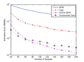
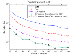
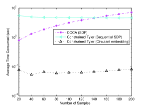
Fig. 1 shows the NMSE of the estimators with β=0.8𝛽0.8\beta=0.8 . The result indicates that the structure constrained Tyler’s estimator achieves the smallest estimation error. In addition, we see that although the circulant embedding algorithm (Algorithm 2) with L=2K1𝐿2𝐾1L=2K-1 approximately solves the Toeplitz structure constrained problem, it achieves virtually the same estimation error as imposing the Toeplitz structure and solving the problem via the sequential SDP algorithm (Algorithm 1). However, the computational cost of circulant embedding is much lower than that of sequential SDP and COCA, as shown in the average time cost plotted in Fig. 2.
Refer to caption
Figure 1: The estimation error (NMSE) of different estimators under the Toeplitz structure of the form (66).
Refer to caption
Figure 2: Average time (in seconds) consumed by COCA and the constrained Tyler’s estimator via sequential SDP (Algorithm 1) and circulant embedding (Algorithm 2).

VI-B Banded Toeplitz Structure

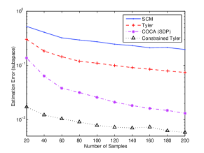
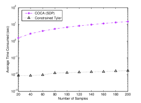
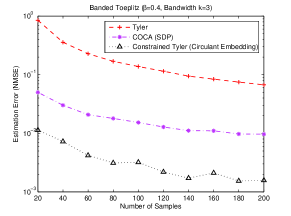
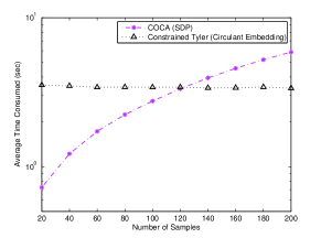
Next we investigate the case that 𝐑0subscript𝐑0{\bf R}_{0} is a k𝑘k-banded Toeplitz matrix Bk(𝐑0)subscript𝐵𝑘subscript𝐑0B_{k}\left({\bf R}_{0}\right), where Bk(𝐑0)subscript𝐵𝑘subscript𝐑0B_{k}\left({\bf R}_{0}\right) defines a matrix with the ij𝑖𝑗ij-th entry equals to that of 𝐑0subscript𝐑0{\bf R}_{0} if |ij|k𝑖𝑗𝑘\left|i-j\right|\leq k, and equals zero otherwise. 𝐑0=𝐑(0.4)subscript𝐑0𝐑0.4{\bf R}_{0}={\bf R}\left(0.4\right) and the bandwidth k𝑘k is chosen to be 333. The NMSE is plotted in Fig. 3, where the constrained Tyler’s estimator achieves the smallest estimation error. Fig. 4 plots the average time consumed by COCA and the constrained Tyler’s estimator. As the number of semidefinite constraints that COCA has is proportional to N𝑁N, the time consumption is approximately linearly increasing in N𝑁N, while the time cost by the algorithm for the constrained Tyler’s estimator remains roughly the same as N𝑁N grows. When N𝑁N is small, the algorithm for COCA runs faster than ours since the scale of the SDP that COCA solves is small. In the regime that N𝑁N is large, the computational cost of COCA increases, as reflected both in the time and the memory required to run the algorithm.
Refer to caption
Figure 3: The estimation error (NMSE) of different estimators under the banded Toeplitz structure.
Refer to caption
Figure 4: Average time (in seconds) consumed by COCA and constrained Tyler’s estimator.

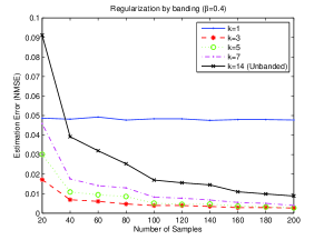
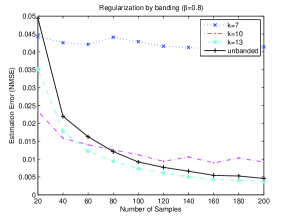
In the third simulation, we consider 𝐑0subscript𝐑0{\bf R}_{0} being a non-banded Toeplitz matrix with the property that (𝐑0)ijsubscriptsubscript𝐑0𝑖𝑗\left({\bf R}_{0}\right)_{ij} decays rapidly as |ij|𝑖𝑗\left|i-j\right| increases. We investigate the cases of 𝐑0=𝐑(0.4)subscript𝐑0𝐑0.4{\bf R}_{0}={\bf R}\left(0.4\right) (fast decay) and 𝐑0=𝐑(0.8)subscript𝐑0𝐑0.8{\bf R}_{0}={\bf R}\left(0.8\right) (slow decay) and impose a banded Toeplitz structure on the Tyler’s estimator with a varying bandwidth k𝑘k to regularize the estimator. Fig. 5 shows that the smallest error is obtained when k=3𝑘3k=3 in the β=0.4𝛽0.4\beta=0.4 case, and when k=13𝑘13k=13 in the β=0.8𝛽0.8\beta=0.8 case. In either case, with the right choice of bandwidth k𝑘k, the regularized estimator outperforms the unbanded one when the number of samples is relatively small compared to the dimension of the covariance matrix to be estimated.
Refer to caption
Refer to caption
Figure 5: NMSE of the regularized Tyler’s estimator by imposing the banded Toeplitz structure of different bandwidth k𝑘k when 𝐑0=𝐑(0.4)subscript𝐑0𝐑0.4{\bf R}_{0}={\bf R}\left(0.4\right) and 𝐑0=𝐑(0.8)subscript𝐑0𝐑0.8{\bf R}_{0}={\bf R}\left(0.8\right).

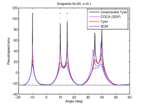
VI-C Direction of Arrival Estimation

In this subsection, we examine the robustness of the proposed estimator in the context of the direction of arrival estimation problem with the following signal model:

𝐱(t)=𝐀𝐬(t)+𝐧(t),𝐱𝑡𝐀𝐬𝑡𝐧𝑡{\bf x}\left(t\right)={\bf A}{\bf s}\left(t\right)+{\bf n}\left(t\right),

where 𝐀=[𝐚(θ1),,𝐚(θL)]𝐀𝐚subscript𝜃1𝐚subscript𝜃𝐿{\bf A}=\left[{\bf a}\left(\theta_{1}\right),\ldots,{\bf a}\left(\theta_{L}\right)\right] is the steering matrix and 𝐧𝐧{\bf n} is zero mean additive noise. We study the simple case of an ideal uniform linear array (ULA) with half-wavelength inter-element spacing, where

𝐚(θ)=[1,ejπsin(θ),,ejπ(K1)sin(θ)]T.𝐚𝜃superscript1superscript𝑒𝑗𝜋𝜃superscript𝑒𝑗𝜋𝐾1𝜃𝑇{\bf a}\left(\theta\right)=\left[1,e^{-j\pi\sin\left(\theta\right)},\ldots,e^{-j\pi\left(K-1\right)\sin\left(\theta\right)}\right]^{T}.

Assuming that the signal 𝐬(t)𝐬𝑡{\bf s}\left(t\right) is a wide-sense stationary random process with zero mean, the covariance of 𝐱(t)𝐱𝑡{\bf x}\left(t\right) is

𝐑=𝐀Cov(𝐬)𝐀H+Cov(𝐧).𝐑𝐀Cov𝐬superscript𝐀𝐻Cov𝐧{\bf R}={\bf A}{\rm Cov}\left({\bf s}\right){\bf A}^{H}+{\rm Cov}\left({\bf n}\right).

Further assume that the signals arriving from different directions are uncorrelated and that the noise is spatially white, i.e., Cov(𝐬)=diag(p1,,pL)Cov𝐬diagsubscript𝑝1subscript𝑝𝐿{\rm Cov}\left({\bf s}\right)={\rm diag}\left(p_{1},\ldots,p_{L}\right) and Cov(𝐧)=σ2𝐈Cov𝐧superscript𝜎2𝐈{\rm Cov}\left({\bf n}\right)=\sigma^{2}{\bf I}, the covariance model simplifies to be

𝐑=j=1Lpj𝐚(θj)𝐚(θj)H+σ2𝐈.𝐑superscriptsubscript𝑗1𝐿subscript𝑝𝑗𝐚subscript𝜃𝑗𝐚superscriptsubscript𝜃𝑗𝐻superscript𝜎2𝐈{\bf R}=\sum_{j=1}^{L}p_{j}{\bf a}\left(\theta_{j}\right){\bf a}\left(\theta_{j}\right)^{H}+\sigma^{2}{\bf I}.

We assume that the number of signals L𝐿L is known in prior.

In our simulation, 5 random signals are assumed arriving from directions 10°10°-10\textdegree, 10°10°10\textdegree, 15°15°15\textdegree, 35°35°35\textdegree, 40°40°40\textdegree with equal power p=1𝑝1p=1 and the noise power is set to be σ2=0.1superscript𝜎20.1\sigma^{2}=0.1. The received signal is assumed to be elliptically distributed. The number of sensors is K=15𝐾15K=15.

We first estimate 𝐑𝐑{\bf R} and then apply the MUSIC algorithm to estimate the arriving angles. The performance of SCM, Tyler’s estimator, COCA and the constrained Tyler’s estimator are compared. For the latter two estimators, 𝐀𝐀{\bf A} is constructed with the θlsubscript𝜃𝑙\theta_{l}’s uniformly located on the interval [π/2,π/2]𝜋2𝜋2\left[-\pi/2,\pi/2\right] with a stepsize of 5°5°5\textdegree. Fig. 6 shows the estimated arrival direction using different estimators with the number of snapshots N=20𝑁20N=20, and only the constrained Tyler’s estimator correctly recovers all of the arriving angles.

Fig. 7 shows the performance of different estimators in terms of NMSE and the estimation error of noise subspace evaluated by

𝐄^c𝐄^cH𝐄c𝐄cHF,subscriptnormsubscript^𝐄𝑐superscriptsubscript^𝐄𝑐𝐻subscript𝐄𝑐superscriptsubscript𝐄𝑐𝐻𝐹\left\|\hat{{\bf E}}_{c}\hat{{\bf E}}_{c}^{H}-{\bf E}_{c}{\bf E}_{c}^{H}\right\|_{F}, (67)

with N𝑁N varying from 20 to 200, where 𝐄csubscript𝐄𝑐{\bf E}_{c} denotes the noise subspace and 𝐄^csubscript^𝐄𝑐\hat{{\bf E}}_{c} denotes its estimate. Fig. 7 (a) reveals that the constrained Tyler’s estimator achieves the smallest NMSE when N𝑁N is small, while COCA performs better when N𝑁N is large. However, Fig. 7 (b) indicates that the constrained Tyler’s estimator can estimate the noise subspace more accurately for all values of N𝑁N, which is beneficial for algorithms that are based on 𝐄^csubscript^𝐄𝑐\hat{{\bf E}}_{c} such as MUSIC.

The average time cost by COCA and the constrained Tyler’s estimator is plotted in Fig. 8. It can be seen that the proposed method is much faster than COCA. In addition, unlike COCA, the consumed time of our algorithm is not sensitive to the number of samples N𝑁N.

Refer to caption
Figure 6: Arrival angle estimated by MUSIC with different covariance estimators.
Refer to caption
(a) NMSE
Refer to caption
(b) Subspace error
Figure 7: The estimation error of different estimators under the DOA structure: (a) NMSE, (b) estimation error of the noise subspace given by different estimators evaluated by (67).
Refer to caption
Figure 8: Average time (in seconds) consumed per data set by COCA and constrained Tyler’s estimator.

VI-D Spiked Covariance Structure

We construct the true covariance 𝐑0subscript𝐑0{\bf R}_{0} by the following model:

𝐑0=j=1Lpj𝐚j𝐚j+Hσ2𝐈,{\bf R}_{0}=\sum_{j=1}^{L}p_{j}{\bf a}_{j}{\bf a}_{j}{}^{H}+\sigma^{2}{\bf I},

where the 𝐚jsubscript𝐚𝑗{\bf a}_{j}’s are randomly generated orthonormal basis and the pjsubscript𝑝𝑗p_{j}’s are randomly generated corresponding eigenvectors uniformly distributed in [0.01,1]0.011\left[0.01,1\right]. σ2superscript𝜎2\sigma^{2} is set to be 0.010.010.01. The number of spikes L=10𝐿10L=10 is assumed to be known in prior. The matrix dimension is fixed to be K=100𝐾100K=100, and the number of samples is varied from N=105𝑁105N=105 to N=150𝑁150N=150. As COCA applies only for convex structural set and cannot be used here, we replace it by the projected Tyler’s estimator, which is a two step procedure that first obtains the Tyler’s estimator and then performs projection according to (53). Fig. 9 shows that imposing the spiked structure helps in reducing the NMSE and subspace estimation error measured by (67).
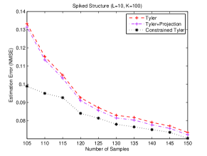
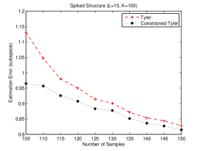
Refer to caption
(a) NMSE
Refer to caption
(b) Subspace error
Figure 9: The estimation error of different estimators under the spiked covariance structure: (a) NMSE, (b) estimation error of the noise subspace given by different estimators evaluated by (67).

VI-E Kronecker Structure

The parameters are set to be 𝐀0=𝐈subscript𝐀0𝐈{\bf A}_{0}={\bf I} , 𝐁0=𝐑(0.8)subscript𝐁0𝐑0.8{\bf B}_{0}={\bf R}\left(0.8\right), p=10𝑝10p=10, q=8𝑞8q=8, in the simulations. We first plot the convergence curve of Algorithms 6 and 7 with the number of samples N=4𝑁4N=4 in Fig. 10. The two algorithms converges in roughly the same number of iterations, and the objective value corresponds to Algorithm 7 (block MM) decreases more smoothly than Algorithm 6 (Gauss-Seidel), as the latter is a double loop algorithm while the former is a single loop algorithm.

Fig. 11 plots the NMSE of Tyler’s estimator with a Kronecker constraint on 𝐑𝐑{\bf R} and that with both a Kronecker constraint on 𝐑𝐑{\bf R} and a Toeplitz constraint on 𝐁𝐁{\bf B}. We can see that further imposing a Toeplitz structure on 𝐁𝐁{\bf B} helps in reducing the estimation error.
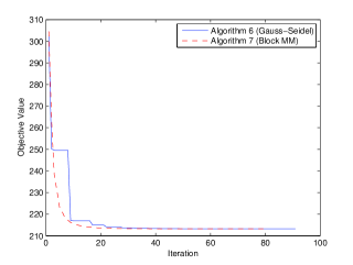
Refer to caption
Figure 10: Convergence Comparison of Algorithm 6 and 7 under the Kronecker structure.
Refer to caption
Figure 11: NMSE of Tyler’s estimator with a Kronecker structural constraint versus that with both a Kronecker and a Toeplitz structural constraint.

VII Conclusion

In this paper, we have discussed the problem of robustly estimating the covariance matrix with a prior structure information. The problem has been formulated as minimizing the negative log-likelihood function of the angular central Gaussian distribution subject to the prior structural constraint. For the general convex constraint, we have proposed a sequential convex programming algorithm based on the majorization minimization framework. The algorithm has been particularized with higher computational efficiency for several specific structures that are widely considered in the signal processing community. The spiked covariance model and the Kronecker structure, although belonging to the non-convex constraint, are also discussed and shown to be computationally tractable. The proposed estimator has been shown outperform the state-of-the-art methods in the numerical section.

References

  • [1] Y. Sun, P. Babu, and D. P. Palomar, “Robust estimation of structured covariance matrix for heavy-tailed distributions,” in Proc. IEEE Int Conf. Acoust., Speech, Signal Process. (ICCASP), 2015.
  • [2] O. Ledoit and M. Wolf, “A well-conditioned estimator for large-dimensional covariance matrices,” J. Multivar. Anal., vol. 88, no. 2, pp. 365 – 411, 2004.
  • [3] P. J. Bickel and E. Levina, “Regularized estimation of large covariance matrices,” Ann. Statist., pp. 199–227, 2008.
  • [4] E. Ollila, D. E. Tyler, V. Koivunen, and H. V. Poor, “Complex elliptically symmetric distributions: Survey, new results and applications,” IEEE Trans. Signal Process., vol. 60, no. 11, pp. 5597–5625, Nov 2012.
  • [5] D. R. Fuhrmann and M. I. Miller, “On the existence of positive-definite maximum-likelihood estimates of structured covariance matrices,” IEEE Trans. Inf. Theory, vol. 34, no. 4, pp. 722–729, 1988.
  • [6] A. Dembo, C. Mallows, and L. Shepp, “Embedding nonnegative definite Toeplitz matrices in nonnegative definite circulant matrices, with application to covariance estimation,” IEEE Trans. Inf. Theory, vol. 35, no. 6, pp. 1206–1212, 1989.
  • [7] M. I. Miller and D. L. Snyder, “The role of likelihood and entropy in incomplete-data problems: applications to estimating point-process intensities and Toeplitz constrained covariances,” Proc. IEEE, vol. 75, no. 7, pp. 892–907, 1987.
  • [8] J. Friedman, T. Hastie, and R. Tibshirani, “Sparse inverse covariance estimation with the graphical lasso,” Biostatistics, vol. 9, no. 3, pp. 432–441, 2008.
  • [9] S. Visuri, H. Oja, and V. Koivunen, “Subspace-based direction-of-arrival estimation using nonparametric statistics,” IEEE Trans. Signal Process., vol. 49, no. 9, pp. 2060–2073, Sep 2001.
  • [10] K. Werner, M. Jansson, and P. Stoica, “On estimation of covariance matrices with Kronecker product structure,” IEEE Trans. Signal Process., vol. 56, no. 2, pp. 478–491, 2008.
  • [11] P. Shah and V. Chandrasekaran, “Group symmetry and covariance regularization,” Electronic Journal of Statistics, vol. 6, pp. 1600–1640, 2012.
  • [12] P. Wirfalt and M. Jansson, “On Kronecker and linearly structured covariance matrix estimation,” IEEE Trans. Signal Process., vol. 62, no. 6, pp. 1536–1547, March 2014.
  • [13] A. M. Zoubir, V. Koivunen, Y. Chakhchoukh, and M. Muma, “Robust estimation in signal processing: A tutorial-style treatment of fundamental concepts,” IEEE Signal Processing Magazine, vol. 29, no. 4, pp. 61–80, 2012.
  • [14] D. B. Williams and D. H. Johnson, “Robust estimation of structured covariance matrices,” IEEE Trans. Signal Process., vol. 41, no. 9, pp. 2891–2906, 1993.
  • [15] D. E. Tyler, “A distribution-free M𝑀M-estimator of multivariate scatter,” Ann. Statist., vol. 15, no. 1, pp. 234–251, 03 1987.
  • [16] I. Soloveychik and A. Wiesel, “Group symmetry and non-Gaussian covariance estimation,” arXiv preprint arXiv:1306.4103, 2013.
  • [17] ——, “Tyler’s covariance matrix estimator in elliptical models with convex structure,” IEEE Trans. Signal Process., vol. 62, no. 20, pp. 5251–5259, Oct 2014.
  • [18] D. E. Tyler, “A distribution-free M𝑀M-estimator of multivariate scatter,” Ann. Statist., vol. 15, no. 1, pp. 234–251, 03 1987.
  • [19] J. T. Kent and D. E. Tyler, “Maximum likelihood estimation for the wrapped Cauchy distribution,” J. Appl. Statist., vol. 15, no. 2, pp. 247–254, 1988.
  • [20] M. Razaviyayn, M. Hong, and Z. Luo, “A unified convergence analysis of block successive minimization methods for nonsmooth optimization,” SIAM J. Optim., vol. 23, no. 2, pp. 1126–1153, 2013.
  • [21] Y. Sun, P. Babu, and D. P. Palomar, “Regularized Tyler’s scatter estimator: Existence, uniqueness, and algorithms,” IEEE Trans. Signal Process., vol. 62, no. 19, pp. 5143–5156, Oct 2014.
  • [22] M. I. Miller and D. L. Snyder, “An alternating maximization of the entropy/likelihood function for image reconstruction and spectrum estimation,” in Proc. SPIE.   San Diego, CA: International Society for Optics and Photonics, 1986, pp. 163–166.
  • [23] I. M. Johnstone, “On the distribution of the largest eigenvalue in principal components analysis,” Ann. Statist., pp. 295–327, 2001.
  • [24] D. Ruppert, Statistics and data analysis for financial engineering.   Springer Science & Business Media, 2010.
  • [25] M. E. Tipping and C. M. Bishop, “Probabilistic principal component analysis,” Journal of the Royal Statistical Society: Series B (Statistical Methodology), vol. 61, no. 3, pp. 611–622, 1999.
  • [26] D. P. Bertsekas, A. Nedić, and A. E. Ozdaglar, Convex analysis and optimization.   Athena Scientific Belmont, 2003.
  • [27] D. P. Bertsekas, Nonlinear Programming.   Athena Scientific, 1999.