Josephson effects in the junction formed by DIII-class topological and $s$-wave superconductors with an embedded quantum dot

Zhen Gao    Wan-Fei Shan    Wei-Jiang Gong gwj@mail.neu.edu.cn 1. College of Sciences, Northeastern University, Shenyang 110819, China
Abstract

We investigate the Josephson effects in the junction formed by DIII-class topological and $s$-wave superconductors, by embedding a quantum dot in the junction. Three dot-superconductor coupling manners are considered, respectively. As a result, the Josephson current is found to oscillate in $2\pi$ period. Moreover, the presence of Majorana doublet in the DIII-class superconductor renders the current finite at the case of zero phase difference, with its sign determined by the fermion parity of such a jucntion. In addition, the dot-superconductor coupling plays a nontrivial role in adjusting the Josephson current. When the $s$-wave superconductor couples to the dot in the weak limit, the current direction will have an opportunity to reverse. The results in this work will be helpful for understanding the transport properties of the DIII-class superconductor.

Time-Reversal Invariant; Topological Superconductor
pacs:
73.21.-b, 74.78.Na, 73.63.-b, 03.67.Lx

I Introduction

Topological superconductors (TSs) have received much attentions from experimental and theoretical aspects because Majorana modes appear at the ends of the one-dimensional TS which can potentially be used for topological quantum computation.Majorana1 ; RMP1 ; Zhang2 Due to the possibility of achieving Majorana modes, the systems with TSs show abundant and interesting physical characteristics.Majorana2 For instance, in the proximity-coupled semiconductor-TS devices, the Majorana zero modes induce the zero-bias anomaly.Fuliang A more compelling TS signature is the unusual Josephson current-phase relation. Namely, when the normal s-wave superconductor nano-wire is replaced by a TS wire with Majorana zero modes, the current-phase relation will be modified to be $I_{J}\sim{\cal P}\sin{\phi\over 2}$ with the period $4\pi$ ($\phi$ is the superconducting phase difference and $\cal P$ is the fermion parity). This is the so-called the fractional Josephson effect.Josephson1 ; Josephson2 ; Josephson3 ; Aguado

More recently, the time-reversal invariant TSs, i.e., the DIII symmetry-class TSs,Ryu ; Qi ; Teo ; Timm ; Beenakker2 have become one new concern.Deng ; Nakosai ; Wong In such a kind of TSs, the zero modes appear in pairs due to Kramers’s theorem, differently from the chiral TSs. Consequently, two Majorana bound states (MBSs) will be localized at each end of the DIII-TS nanowire, leading to the formation of one Kramers doublet.Zhang ; Nagaosa2 Since the Kramers doublet is protected by the time-reversal symmetry, it will inevitably drive some new transport phenomena, opposite to the single Majorana zero mode. Up to now, many groups have proposed proposals to achieve the DIII-TS nanowires, by using the proximity effects of $d$-wave, $p$-wave, $s\pm$-wave, or conventional $s$-wave superconductors.Stern ; Flensberg ; Haim ; ZhangF2 ; Sau ; Loss Meanwhile, physicists have paid attention to the quantum transport phenomena contributed by the Kramers doublet, and some important results have been reported.Qixl ; Liuxj ; Gong1 For instance, in the Josephson junction formed by the Majorana doublet, the period of the Josephson current will be varied by the change of fermion parity in this system.Liuxj This exactly embodies the nontrivial role of Majorana doublet in contributing to the Josephson effect. However, for further understanding the property of Majorana doublet, Josephson effects in any new junctions should be investigated.

In this work, we would like to discuss the Josephson effect in a complicate junction, i.e., one junction formed by the indirect coupling between a DIII-class TS and $s$-wave superconductor with one embedded quantum dot (QD). Our calculations show that the interplay between the DIII-class TS and the $s$-wave superconductor induce interesting results. Although the Josephson current oscillates in $2\pi$ period, the presence of Majorana doublet in the DIII-class TS renders it finite at the case of zero phase difference, with its sign determined by the fermion parity of the whole system. Also, QD plays a nontrivial role in adjusting the Josephson effect. To be concrete, in the extreme case where the $s$-wave superconductor couples weakly to the QD, the direction of the Josephson current will be reversed. All these results embodies the specific role of DIII-class TS in driving the Josephson effect.

Refer to caption
Figure 1: The junction formed by DIII-class topological and $s$-wave superconductors. One QD is embedded in the junction.

II Theoretical model

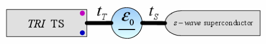
The considered Josephson junction is illustrated in Fig.1, where one DIII-class TS couples to one $s$-wave superconductor via one QD. The Hamiltonian of such a system can be written as $H=H_{p}+H_{s}+H_{D}+H_{T}$. The first two terms, i.e., $H_{p}$ and $H_{s}$, denote the Hamiltonians of the DIII-class TS and s-wave superconductor respectively, which is written asQixl

$\displaystyle H_{p}$ $\displaystyle=$ βˆ’ΞΌpβ€‹βˆ‘j​σcj​σ†​cjβ€‹Οƒβˆ’tβ€‹βˆ‘j​σ(cj+1,σ†​cj​σ+h.c.)+βˆ‘j​σ​σ′[(βˆ’i​σ1​σ2)σ​σ′​Δp​cj+1,σ†​cj​σ†+h.c.],subscriptπœ‡π‘subscriptπ‘—πœŽsuperscriptsubscriptπ‘π‘—πœŽβ€ subscriptπ‘π‘—πœŽπ‘‘subscriptπ‘—πœŽsuperscriptsubscript𝑐𝑗1πœŽβ€ subscriptπ‘π‘—πœŽh.c.subscriptπ‘—πœŽsuperscriptπœŽβ€²delimited-[]subscript𝑖subscript𝜎1subscript𝜎2𝜎superscriptπœŽβ€²subscriptΔ𝑝superscriptsubscript𝑐𝑗1πœŽβ€ superscriptsubscriptπ‘π‘—πœŽβ€ h.c.\displaystyle-\mu_{p}\sum_{j\sigma}c_{j\sigma}^{\dagger}c_{j\sigma}-t\sum_{j\sigma}(c_{j+1,\sigma}^{\dagger}c_{j\sigma}+\text{h.c.})+\sum_{j\sigma\sigma^{\prime}}[(-i\sigma_{1}\sigma_{2})_{\sigma\sigma^{\prime}}\Delta_{p}c_{j+1,\sigma}^{\dagger}c_{j\sigma}^{\dagger}+\text{h.c.}],
$\displaystyle H_{s}$ $\displaystyle=$ βˆ’ΞΌsβ€‹βˆ‘j​σfj​σ†​fjβ€‹Οƒβˆ’tβ€²β€‹βˆ‘j​σ(fj+1,σ†​fj​σ+h.c.)+βˆ‘j(Ξ”s​fj↑†​fj↓†+h.c.).subscriptπœ‡π‘ subscriptπ‘—πœŽsuperscriptsubscriptπ‘“π‘—πœŽβ€ subscriptπ‘“π‘—πœŽsuperscript𝑑′subscriptπ‘—πœŽsuperscriptsubscript𝑓𝑗1πœŽβ€ subscriptπ‘“π‘—πœŽh.c.subscript𝑗subscriptΔ𝑠superscriptsubscript𝑓↑𝑗absent†superscriptsubscript𝑓↓𝑗absent†h.c.\displaystyle-\mu_{s}\sum_{j\sigma}f_{j\sigma}^{\dagger}f_{j\sigma}-t^{\prime}\sum_{j\sigma}(f_{j+1,\sigma}^{\dagger}f_{j\sigma}+\text{h.c.})+\sum_{j}(\Delta_{s}f_{j\uparrow}^{\dagger}f_{j\downarrow}^{\dagger}+\text{h.c.}). (1)

cj​σ†subscriptsuperscriptπ‘β€ π‘—πœŽc^{\dagger}_{j\sigma} and fj​σ†subscriptsuperscriptπ‘“β€ π‘—πœŽf^{\dagger}_{j\sigma} ($c_{j\sigma}$ and $f_{j\sigma}$) are the electron creation (annihilation) operators in the DIII-class TS and $s$-wave superconductor, respectively. $\mu_{p}$ and ΞΌssubscriptπœ‡π‘ \mu_{s} are the chemical potentials of the superconductors, and $\Delta_{p}$ and $\Delta_{s}$ are the Copper-pair hopping terms. $H_{D}$ describes the Hamiltonian of the QD. For a single-level QD, it takes the form as $H_{D}=H_{d0}+H_{ee}$ with

$\displaystyle H_{d0}=\varepsilon_{0}\sum_{\sigma}(n_{\sigma}-{1\over 2}),~{}H_{ee}=U(n_{\uparrow}-{1\over 2})(n_{\downarrow}-{1\over 2}).$ (2)

nΟƒ=dσ†​dΟƒsubscriptπ‘›πœŽsubscriptsuperscriptπ‘‘β€ πœŽsubscriptπ‘‘πœŽn_{\sigma}=d^{\dagger}_{\sigma}d_{\sigma} is the electron-number operator, in which dσ†subscriptsuperscriptπ‘‘β€ πœŽd^{\dagger}_{\sigma} and $d_{\sigma}$ are the creation and annihilation operators in the QD. $\varepsilon_{0}$ is the QD level, and $U$ denotes the intradot Coulomb repulsion. $H_{T}$, the last term of $H$, represents the couplings between the QD and the superconductors. It can be given by

$\displaystyle H_{T}$ =βˆ’tTβ€‹βˆ‘Οƒ(ei​θT/2​c1​σ†​dΟƒ+h.c.)βˆ’tSβ€‹βˆ‘Οƒ(ei​θS/2​f1​σ†​dΟƒ+h.c.),absentsubscript𝑑𝑇subscript𝜎superscript𝑒𝑖subscriptπœƒπ‘‡2superscriptsubscript𝑐1πœŽβ€ subscriptπ‘‘πœŽh.c.subscript𝑑𝑆subscript𝜎superscript𝑒𝑖subscriptπœƒπ‘†2superscriptsubscript𝑓1πœŽβ€ subscriptπ‘‘πœŽh.c.\displaystyle=-t_{T}\sum_{\sigma}(e^{i\theta_{T}/2}c_{1\sigma}^{\dagger}d_{\sigma}+\text{h.c.})-t_{S}\sum_{\sigma}(e^{i\theta_{S}/2}f_{1\sigma}^{\dagger}d_{\sigma}+\text{h.c.}), (3)

where $t_{T}$ and $t_{S}$ are the QD-superconductor coupling coefficients, respectively.

It is well-known that the phase difference between superconductors drives finite current through one Josephson junction. With respect to such a junction, the current properties can be evaluated by the following formula

$$I_{J}={2e\over\hbar}{\partial{\langle H}\rangle\over\partial\theta}.$$ (4)

In this equation $\theta=\theta_{T}-\theta_{S}$ is the phase difference between the superconductors, and $\langle\cdots\rangle$ is the thermal average. As a typical case, i.e., the zero-temperature limit, the Josephson current can be simplified as

$$I_{J}={2e\over\hbar}{\partial E_{GS}\over\partial\theta}.$$ (5)

This formula shows that the calculation about the Josephson current is dependent on the ground-state (GS) level of this system.

In the low-energy region, DIII-class TS only contributes Majorana doublets to the Josephson effect, so $H_{p}$ describes the coupling between two Majorana doublets. For the extreme case of one infinitely-long TS, the coupling strength between the Majorana doublets decreases to zero.LossN Following this idea, we project $H_{T}$ onto its zero-energy subspace. As a result, $H$ can be rewritten as

$\displaystyle H$ $\displaystyle=$ Ξ΅0β€‹βˆ‘Οƒ(nΟƒβˆ’12)+U​(nβ†‘βˆ’12)​(nβ†“βˆ’12)+βˆ‘k​σξk​fk​σ†​fk​σ+Ξ”sβ€‹βˆ‘kfk↑†​fβˆ’k↓†subscriptπœ€0subscript𝜎subscriptπ‘›πœŽ12π‘ˆsubscript𝑛↑12subscript𝑛↓12subscriptπ‘˜πœŽsubscriptπœ‰π‘˜subscriptsuperscriptπ‘“β€ π‘˜πœŽsubscriptπ‘“π‘˜πœŽsubscriptΔ𝑠subscriptπ‘˜subscriptsuperscriptπ‘“β€ β†‘π‘˜absentsubscriptsuperscriptπ‘“β€ β†“π‘˜absent\displaystyle\varepsilon_{0}\sum_{\sigma}(n_{\sigma}-{1\over 2})+U(n_{\uparrow}-{1\over 2})(n_{\downarrow}-{1\over 2})+\sum_{k\sigma}\xi_{k}f^{\dagger}_{k\sigma}f_{k\sigma}+\Delta_{s}\sum_{k}f^{\dagger}_{k\uparrow}f^{\dagger}_{-k\downarrow} (6)
+tTβ€‹βˆ‘Οƒ(ei​θ/2​dΟƒβˆ’eβˆ’i​θ/2​dσ†)​γ0β€‹Οƒβˆ’βˆ‘k​σVk​S​fk​σ†​dΟƒ+h.c.,subscript𝑑𝑇subscript𝜎superscriptπ‘’π‘–πœƒ2subscriptπ‘‘πœŽsuperscriptπ‘’π‘–πœƒ2superscriptsubscriptπ‘‘πœŽβ€ subscript𝛾0𝜎subscriptπ‘˜πœŽsubscriptπ‘‰π‘˜π‘†superscriptsubscriptπ‘“π‘˜πœŽβ€ subscriptπ‘‘πœŽh.c.\displaystyle+t_{T}\sum_{\sigma}(e^{i\theta/2}d_{\sigma}-e^{-i\theta/2}d_{\sigma}^{\dagger})\gamma_{0\sigma}-\sum_{k\sigma}V_{kS}f_{k\sigma}^{\dagger}d_{\sigma}+\text{h.c.},

where $H_{s}$ has been projected into in the Bloch space with $\xi_{k}=-\mu^{\prime}-2t^{\prime}\cos k$ and $V_{kS}={1\over\sqrt{N}}\sum_{k}e^{ik}t_{S}$. $\gamma_{0\sigma}$, the Majorana operator, which obeys the anti-commutation relationship of $\{\gamma_{0\sigma},\gamma_{0\sigma^{\prime}}\}=2\delta_{\sigma\sigma^{\prime}}$. Based on the renewed expression of $H$, we next try to diagonalize the Hamiltonian of such a Josephson junction.

III Diagonalization of the junction Hamiltonian

The continuum state in the $s$-wave superconductor hinders the diagonalization of the system’s Hamiltonian. In order to present a comprehensive analysis, we would like to consider three cases, i.e., the cases of $t_{T}\gg t_{S}$, $t_{T}\approx t_{S}$, and $t_{T}\ll t_{S}$, followed by the utilization of different approximation methods. The following are the detailed discussion processes. For convenience, they are named as Case I, Case II, and Case III, respectively.

III.1 Diagonalization of $H$ in Case I

In Case I where $t_{T}\gg t_{S}$, the subsystem formed by the QD and Majorana doublet can be considered to be one system, whereas the $s$-wave superconductor can be viewed as a perturbation factor. We next simplify the system Hamiltonian by means of the perturbation theory. Ignoring the Coulomb interaction term in the QD, we can write out the action of the subsystem of QD and $s$-wave superconductor

$\displaystyle S$ $\displaystyle=$ βˆ«π‘‘Ο„β€‹[Ξ¨d†​(βˆ‚Ο„+β„‹d​0)​Ψd]+βˆ«π‘‘Ο„β€‹βˆ‘k{Ξ¨k†​[βˆ‚Ο„+β„‹s​(k)]​Ψkβˆ’[Ξ¨d†​𝒱k​S​Ψk+Ξ¨k†​𝒱k​S†​Ψd]},differential-d𝜏delimited-[]superscriptsubscriptΨ𝑑†subscript𝜏subscriptℋ𝑑0subscriptΨ𝑑differential-d𝜏subscriptπ‘˜superscriptsubscriptΞ¨π‘˜β€ delimited-[]subscript𝜏subscriptβ„‹π‘ π‘˜subscriptΞ¨π‘˜delimited-[]superscriptsubscriptΨ𝑑†subscriptπ’±π‘˜π‘†subscriptΞ¨π‘˜superscriptsubscriptΞ¨π‘˜β€ subscriptsuperscriptπ’±β€ π‘˜π‘†subscriptΨ𝑑\displaystyle\int d\tau\,[\Psi_{d}^{\dagger}(\partial_{\tau}+\mathcal{H}_{d0})\Psi_{d}]+\int d\tau\sum_{k}\{\Psi_{k}^{\dagger}[\partial_{\tau}+\mathcal{H}_{s}(k)]\Psi_{k}-[\Psi_{d}^{\dagger}{\cal V}_{kS}\Psi_{k}+\Psi_{k}^{\dagger}{\cal V}^{\dagger}_{kS}\Psi_{d}]\}, (7)

where ${\cal H}_{d0}=\varepsilon_{0}\sigma_{z}$, ${\cal H}_{s}=\xi_{k}\sigma_{z}+\Delta_{s}\sigma_{x}$, and ${\cal V}_{kS}=V_{kS}\sigma_{z}$. As for the field operators, they are given by $\Psi_{d}=\left[\begin{array}[]{c}d_{\uparrow}\\ d_{\downarrow}^{\dagger}\\ \end{array}\right]$ and Ξ¨k=[fk↑fβˆ’k↓†]subscriptΞ¨π‘˜delimited-[]subscriptπ‘“β†‘π‘˜absentsubscriptsuperscriptπ‘“β€ β†“π‘˜absent\Psi_{k}=\left[\begin{array}[]{c}f_{k\uparrow}\\ f^{\dagger}_{-k\downarrow}\\ \end{array}\right]. With the action $S$, we can express the partition function as a path integral, i.e., Z=Tr​[eβˆ’Ξ²β€‹H]=βˆ«π’Ÿβ€‹Ξ¨kβ€‹π’Ÿβ€‹Ξ¨k†​eβˆ’S𝑍Trdelimited-[]superscriptπ‘’π›½π»π’ŸsubscriptΞ¨π‘˜π’ŸsuperscriptsubscriptΞ¨π‘˜β€ superscript𝑒𝑆Z={\rm Tr}[e^{-\beta H}]=\int\mathcal{D}\Psi_{k}\mathcal{D}\Psi_{k}^{\dagger}e^{-S}, in which the measure $\mathcal{D}\Psi_{k}$ denotes all the possible integral paths. After integrating out the fermion field Ξ¨k,Ξ¨k†subscriptΞ¨π‘˜subscriptsuperscriptΞ¨β€ π‘˜\Psi_{k},\Psi^{\dagger}_{k} with a Gaussian integral, the partition function will become a β€œgenerating functional”

$\displaystyle Z[\Psi_{d},\Psi_{d}^{\dagger}]$ =det[βˆ‚Ο„+β„‹d​0]​exp⁑[βˆ«π‘‘Ο„β€‹π‘‘Ο„β€²β€‹βˆ‘kΞ¨d†​(Ο„)​𝒱k​S​G​(k,Ο„βˆ’Ο„β€²)​𝒱k​S†​Ψd​(Ο„β€²)].absentdelimited-[]subscript𝜏subscriptℋ𝑑0differential-d𝜏differential-dsuperscriptπœβ€²subscriptπ‘˜superscriptsubscriptΞ¨π‘‘β€ πœsubscriptπ’±π‘˜π‘†Gπ‘˜πœsuperscriptπœβ€²subscriptsuperscriptπ’±β€ π‘˜π‘†subscriptΨ𝑑superscriptπœβ€²\displaystyle=\det[\partial_{\tau}+\mathcal{H}_{d0}]\exp\left[\int d\tau d\tau^{\prime}\sum_{k}\Psi_{d}^{\dagger}(\tau){\cal V}_{kS}\textbf{G}(k,\tau-\tau^{\prime}){\cal V}^{\dagger}_{kS}\Psi_{d}(\tau^{\prime})\right]. (8)

G​(k,Ο„βˆ’Ο„β€²)=βˆ’βŸ¨Tτ​Ψk​(Ο„)βŠ—Ξ¨k†​(Ο„β€²)⟩Gπ‘˜πœsuperscriptπœβ€²delimited-⟨⟩tensor-productsubscriptπ‘‡πœsubscriptΞ¨π‘˜πœsuperscriptsubscriptΞ¨π‘˜β€ superscriptπœβ€²\textbf{G}(k,\tau-\tau^{\prime})=-\langle T_{\tau}\Psi_{k}(\tau)\otimes\Psi_{k}^{\dagger}(\tau^{\prime})\rangle is defined in the $s$-wave superconductor. It obeys the Fourier expansion $\textbf{G}(k,\tau)={1\over\beta}\sum_{n}e^{-i\omega_{n}\tau}\textbf{G}(k,i\omega_{n})$ with $\textbf{G}(k,i\omega_{n})=[\det(i\omega_{n}-\mathcal{H}_{s})]^{-1}\left[\begin{array}[]{cc}i\omega_{n}+\xi_{k}&\Delta_{s}e^{i\theta}\\ \Delta_{s}e^{-i\theta}&i\omega_{n}-\xi_{k}\\ \end{array}\right]$. This allows us to write out the effective expression of the action in the Fourier space directly, i.e.,

$\displaystyle S_{\text{eff}}$ $\displaystyle=-\sum_{i\omega_{n}}\text{Tr}\ln G^{-1}_{d0}(i\omega_{n})-\frac{t_{S}^{2}}{\beta}\sum_{k,i\omega_{n}}\Psi_{d}^{\dagger}\textbf{G}(k,i\omega_{n})\Psi_{d}$ (9)
$\displaystyle=-\sum_{i\omega_{n}}\ln\left[\omega_{n}^{2}+\varepsilon_{0}^{2}\right]-\frac{t_{S}^{2}}{\beta}\sum_{k}\Psi_{d}^{\dagger}[\frac{i\omega_{n}\sigma_{0}+\xi_{k}\sigma_{z}+\Delta_{s}\sigma_{x}}{\omega_{n}^{2}+\xi_{k}^{2}+\Delta_{s}^{2}}]\Psi_{d}.$

With the help of the expression of $S_{\text{eff}}$, it is not difficult for us to get the perturbative Hamiltonian of the $s$-wave superconductor on the QD

$\displaystyle H^{\prime}\simeq-\frac{t_{S}^{2}}{N}\sum_{k}\Psi_{d}^{\dagger}[\frac{\xi_{k}}{\xi_{k}^{2}+\Delta_{s}^{2}}\sigma_{z}+\frac{\Delta_{s}}{\xi_{k}^{2}+\Delta_{s}^{2}}\sigma_{x}]\Psi_{d}.$ (10)

Via a unitary transformation, the system Hamiltonian can be expressed as the following form

Heff=Ξ΅0β€‹βˆ‘Οƒ(nΟƒβˆ’12)+Ξ”~s​(ei​θ​d↑†​d↓†+eβˆ’i​θ​d↓​d↑)+U​(nβ†‘βˆ’12)​(nβ†“βˆ’12)+tTβ€‹βˆ‘Οƒ(dΟƒβˆ’dσ†)​γ0​σ,subscript𝐻effsubscriptπœ€0subscript𝜎subscriptπ‘›πœŽ12subscript~Δ𝑠superscriptπ‘’π‘–πœƒsuperscriptsubscript𝑑↑†superscriptsubscript𝑑↓†superscriptπ‘’π‘–πœƒsubscript𝑑↓subscriptπ‘‘β†‘π‘ˆsubscript𝑛↑12subscript𝑛↓12subscript𝑑𝑇subscript𝜎subscriptπ‘‘πœŽsuperscriptsubscriptπ‘‘πœŽβ€ subscript𝛾0𝜎\displaystyle H_{\rm eff}=\varepsilon_{0}\sum_{\sigma}(n_{\sigma}-{1\over 2})+\tilde{\Delta}_{s}(e^{i\theta}d_{\uparrow}^{\dagger}d_{\downarrow}^{\dagger}+e^{-i\theta}d_{\downarrow}d_{\uparrow})+U(n_{\uparrow}-{1\over 2})(n_{\downarrow}-{1\over 2})+t_{T}\sum_{\sigma}(d_{\sigma}-d_{\sigma}^{\dagger})\gamma_{0\sigma}, (11)

with $\tilde{\Delta}_{s}={t_{S}^{2}\over N}\sum_{k}{\Delta_{s}\over\xi_{k}^{2}+\Delta_{s}^{2}}$. Such a result indicates that the weak Andreev reflection between the $s$-wave superconductor and QD induces a weak $s$-wave pairing potential on the QD, which is exactly the so-called the proximity effect.

For the sake of diagonalizing such a Hamiltonian, we need to introduce local Majorana operators Ξ·i​ssubscriptπœ‚π‘–π‘ \eta_{is} through $d_{\sigma}=\frac{1}{\sqrt{2}}(\eta_{1\sigma}+i\eta_{2\sigma})$ and dσ†=12​(Ξ·1β€‹Οƒβˆ’i​η2​σ)superscriptsubscriptπ‘‘πœŽβ€ 12subscriptπœ‚1πœŽπ‘–subscriptπœ‚2𝜎d_{\sigma}^{\dagger}=\frac{1}{\sqrt{2}}(\eta_{1\sigma}-i\eta_{2\sigma}). And then, by defining Dirac fermionic operators $a=\frac{1}{\sqrt{2}}(\eta_{1\uparrow}+i\eta_{1\downarrow})$, $b=\frac{i}{\sqrt{2}}(\eta_{2\uparrow}+i\eta_{2\downarrow})$, and $\tilde{f}=\frac{1}{\sqrt{2}}(\gamma_{0\uparrow}+i\gamma_{0\downarrow})$, we can obtain a new expression of $H_{\rm eff}$, i.e.,

$\displaystyle H_{\rm eff}$ $\displaystyle=$ Ξ”~s​sin⁑θ​(a†​aβˆ’b†​b)+(Ξ΅0+i​Δ~s​cos⁑θ)​a†​b+(Ξ΅0βˆ’i​Δ~s​cos⁑θ)​b†​asubscript~Ξ”π‘ πœƒsuperscriptπ‘Žβ€ π‘Žsuperscript𝑏†𝑏subscriptπœ€0𝑖subscript~Ξ”π‘ πœƒsuperscriptπ‘Žβ€ π‘subscriptπœ€0𝑖subscript~Ξ”π‘ πœƒsuperscriptπ‘β€ π‘Ž\displaystyle\tilde{\Delta}_{s}\sin\theta(a^{\dagger}a-b^{\dagger}b)+(\varepsilon_{0}+i\tilde{\Delta}_{s}\cos\theta)a^{\dagger}b+(\varepsilon_{0}-i\tilde{\Delta}_{s}\cos\theta)b^{\dagger}a (12)
$\displaystyle-U(n_{a}-{1\over 2})(n_{b}-{1\over 2})-\sqrt{2}t_{T}(b^{\dagger}\tilde{f}+h.c.).$

According to Eq.(12), the Bogoliubov Cde Gennes equation $H_{\rm eff}\Psi=E\Psi$ can be built, and then the eigenvalues of $H_{\rm eff}$ can be worked out. On the basis of $\{|000\rangle,|001\rangle,|010\rangle,|100\rangle,|110\rangle,|101\rangle,|011\rangle,|111\rangle\}$, the matrix form of $H$ can be obtained ($|n_{a}n_{b}n_{f}\rangle=|n_{a}\rangle|n_{b}\rangle|n_{\tilde{f}}\rangle$, where na=a†​asubscriptπ‘›π‘Žsuperscriptπ‘Žβ€ π‘Žn_{a}=a^{\dagger}a, $n_{b}=b^{\dagger}b$, and $n_{\tilde{f}}=\tilde{f}^{\dagger}\tilde{f}$). Note that in the TS-existed system, only the parity of the average particle occupation number is the good quantum number, thus the matrix form of $H_{\rm eff}$ should be given according to fermion parity (FP). In the case of odd FP, $\Psi_{o}=c_{1}|001\rangle+c_{2}|010\rangle+c_{3}|100\rangle+c_{4}|111\rangle$, and then

Heff(o)=[βˆ’U4βˆ’2​tT00βˆ’2​tTβˆ’Ξ”~s​sin⁑θ+U4Ξ΅0βˆ’i​Δ~s​cos⁑θ00Ξ΅0+i​Δ~s​cos⁑θΔ~s​sin⁑θ+U40000βˆ’U4];subscriptsuperscriptπ»π‘œeffdelimited-[]π‘ˆ42subscript𝑑𝑇002subscript𝑑𝑇subscript~Ξ”π‘ πœƒπ‘ˆ4subscriptπœ€0𝑖subscript~Ξ”π‘ πœƒ00subscriptπœ€0𝑖subscript~Ξ”π‘ πœƒsubscript~Ξ”π‘ πœƒπ‘ˆ40000π‘ˆ4\displaystyle H^{(o)}_{\rm eff}=\left[\begin{array}[]{cccc}-{U\over 4}&-\sqrt{2}t_{T}&0&0\\ -\sqrt{2}t_{T}&-\tilde{\Delta}_{s}\sin\theta+{U\over 4}&\varepsilon_{0}-i\tilde{\Delta}_{s}\cos\theta&0\\ 0&\varepsilon_{0}+i\tilde{\Delta}_{s}\cos\theta&\tilde{\Delta}_{s}\sin\theta+{U\over 4}&0\\ 0&0&0&-{U\over 4}\end{array}\right]; (17)

In the case of even FP, $\Psi_{e}=c_{1}|000\rangle+c_{2}|011\rangle+c_{3}|101\rangle+c_{4}|110\rangle$, and

Heff(e)=[βˆ’U40000βˆ’Ξ”~s​sin⁑θ+U4Ξ΅0βˆ’i​Δ~s​cos⁑θ00Ξ΅0+i​Δ~s​cos⁑θΔ~s​sin⁑θ+U4βˆ’2​tT00βˆ’2​tTβˆ’U4].subscriptsuperscript𝐻𝑒effdelimited-[]π‘ˆ40000subscript~Ξ”π‘ πœƒπ‘ˆ4subscriptπœ€0𝑖subscript~Ξ”π‘ πœƒ00subscriptπœ€0𝑖subscript~Ξ”π‘ πœƒsubscript~Ξ”π‘ πœƒπ‘ˆ42subscript𝑑𝑇002subscriptπ‘‘π‘‡π‘ˆ4\displaystyle H^{(e)}_{\rm eff}=\left[\begin{array}[]{cccc}-{U\over 4}&0&0&0\\ 0&-\tilde{\Delta}_{s}\sin\theta+{U\over 4}&\varepsilon_{0}-i\tilde{\Delta}_{s}\cos\theta&0\\ 0&\varepsilon_{0}+i\tilde{\Delta}_{s}\cos\theta&\tilde{\Delta}_{s}\sin\theta+{U\over 4}&-\sqrt{2}t_{T}\\ 0&0&-\sqrt{2}t_{T}&-{U\over 4}\end{array}\right]. (22)

It is easy to find that $H^{(o)}_{\rm eff}(\theta)=H^{(e)}_{\rm eff}(\theta+\pi)$. Thus, the Josephson effect can be clarified by only analyzing the current oscillation result in one FP.

III.2 Diagonalization of $H$ in Case II

In Case II where $t_{T}\approx t_{S}$, $H$ is difficult to diagonalize due to the presence of continuum state in the $s$-wave superconductor. However, according to the previous works, the zero band-width approximation is feasible to solve the Josephson effect contributed by the $s$-wave superconductor.ZBA Within such an approximation, the Hamiltonian can be simplified as

$\displaystyle H_{\rm eff}$ $\displaystyle=$ Ξ΅0β€‹βˆ‘Οƒ(nΟƒβˆ’12)+U​(nβ†‘βˆ’12)​(nβ†“βˆ’12)+βˆ‘ΟƒΞΎβ€‹fσ†​fΟƒ+Ξ”s​(ei​θ​f↑†​f↓†+eβˆ’i​θ​f↓​f↑)subscriptπœ€0subscript𝜎subscriptπ‘›πœŽ12π‘ˆsubscript𝑛↑12subscript𝑛↓12subscriptπœŽπœ‰subscriptsuperscriptπ‘“β€ πœŽsubscriptπ‘“πœŽsubscriptΔ𝑠superscriptπ‘’π‘–πœƒsubscriptsuperscript𝑓†↑subscriptsuperscript𝑓†↓superscriptπ‘’π‘–πœƒsubscript𝑓↓subscript𝑓↑\displaystyle\varepsilon_{0}\sum_{\sigma}(n_{\sigma}-{1\over 2})+U(n_{\uparrow}-{1\over 2})(n_{\downarrow}-{1\over 2})+\sum_{\sigma}\xi f^{\dagger}_{\sigma}f_{\sigma}+\Delta_{s}(e^{i\theta}f^{\dagger}_{\uparrow}f^{\dagger}_{\downarrow}+e^{-i\theta}f_{\downarrow}f_{\uparrow}) (23)
+tTβ€‹βˆ‘Οƒ(dΟƒβˆ’dσ†)​γ0β€‹Οƒβˆ’βˆ‘ΟƒtS​fσ†​dΟƒ+h.c..subscript𝑑𝑇subscript𝜎subscriptπ‘‘πœŽsuperscriptsubscriptπ‘‘πœŽβ€ subscript𝛾0𝜎subscript𝜎subscript𝑑𝑆superscriptsubscriptπ‘“πœŽβ€ subscriptπ‘‘πœŽh.c.\displaystyle+t_{T}\sum_{\sigma}(d_{\sigma}-d_{\sigma}^{\dagger})\gamma_{0\sigma}-\sum_{\sigma}t_{S}f_{\sigma}^{\dagger}d_{\sigma}+\text{h.c.}.

By defining $f_{\sigma}=\frac{1}{\sqrt{2}}(\zeta_{1\sigma}+i\zeta_{2\sigma})$ and fσ†=12​(ΞΆ1β€‹Οƒβˆ’i​΢2​σ)superscriptsubscriptπ‘“πœŽβ€ 12subscript𝜁1πœŽπ‘–subscript𝜁2𝜎f_{\sigma}^{\dagger}=\frac{1}{\sqrt{2}}(\zeta_{1\sigma}-i\zeta_{2\sigma}) with $\alpha=\frac{1}{\sqrt{2}}(\zeta_{1\uparrow}+i\zeta_{1\downarrow})$ and $\beta=\frac{i}{\sqrt{2}}(\zeta_{2\uparrow}+i\zeta_{2\downarrow})$, we get the Hamiltonian in the spinless-fermion representation

$\displaystyle H_{\rm eff}$ $\displaystyle=$ Ξ΅0​(a†​b+b†​a)βˆ’U​(naβˆ’12)​(nbβˆ’12)subscriptπœ€0superscriptπ‘Žβ€ π‘superscriptπ‘β€ π‘Žπ‘ˆsubscriptπ‘›π‘Ž12subscript𝑛𝑏12\displaystyle\varepsilon_{0}(a^{\dagger}b+b^{\dagger}a)-U(n_{a}-{1\over 2})(n_{b}-{1\over 2}) (24)
+Ξ”s​sin⁑θ​(Ξ±β€ β€‹Ξ±βˆ’Ξ²β€ β€‹Ξ²)+(ΞΎ+i​Δs​cos⁑θ)​α†​β+(ΞΎβˆ’i​Δs​cos⁑θ)​β†​αsubscriptΞ”π‘ πœƒsuperscript𝛼†𝛼superscriptπ›½β€ π›½πœ‰π‘–subscriptΞ”π‘ πœƒsuperscriptπ›Όβ€ π›½πœ‰π‘–subscriptΞ”π‘ πœƒsuperscript𝛽†𝛼\displaystyle+\Delta_{s}\sin\theta(\alpha^{\dagger}\alpha-\beta^{\dagger}\beta)+(\xi+i\Delta_{s}\cos\theta)\alpha^{\dagger}\beta+(\xi-i\Delta_{s}\cos\theta)\beta^{\dagger}\alpha
βˆ’2​tT​(b†​f~+f~†​b)βˆ’tS​(b†​α+α†​b+a†​β+β†​a).2subscript𝑑𝑇superscript𝑏†~𝑓superscript~𝑓†𝑏subscript𝑑𝑆superscript𝑏†𝛼superscript𝛼†𝑏superscriptπ‘Žβ€ π›½superscriptπ›½β€ π‘Ž\displaystyle-\sqrt{2}t_{T}(b^{\dagger}\tilde{f}+\tilde{f}^{\dagger}b)-t_{S}(b^{\dagger}\alpha+\alpha^{\dagger}b+a^{\dagger}\beta+\beta^{\dagger}a).

On the basis of odd FP, the matrix of $H^{(o)}_{\rm eff}$ can be expressed as

$\displaystyle H^{(o)}_{\rm eff}=\left[\begin{array}[]{ccc}h^{(o)}_{I}&0&0\\ 0&h^{(o)}_{III}&0\\ 0&0&-{U\over 4}\end{array}\right],$ (28)

where

hI(o)=[U4Ξ΅00βˆ’tS0Ξ΅0U4βˆ’tS0βˆ’2​tT0βˆ’tSΞ”s​sinβ‘ΞΈβˆ’U4ΞΎ+i​Δs​cos⁑θ0βˆ’tS0ΞΎβˆ’i​Δs​cosβ‘ΞΈβˆ’Ξ”s​sinβ‘ΞΈβˆ’U400βˆ’2​tT00βˆ’U4]subscriptsuperscriptβ„Žπ‘œπΌdelimited-[]π‘ˆ4subscriptπœ€00subscript𝑑𝑆0missing-subexpressionmissing-subexpressionsubscriptπœ€0π‘ˆ4subscript𝑑𝑆02subscript𝑑𝑇missing-subexpressionmissing-subexpression0subscript𝑑𝑆subscriptΞ”π‘ πœƒπ‘ˆ4πœ‰π‘–subscriptΞ”π‘ πœƒ0missing-subexpressionmissing-subexpressionsubscript𝑑𝑆0πœ‰π‘–subscriptΞ”π‘ πœƒsubscriptΞ”π‘ πœƒπ‘ˆ40missing-subexpressionmissing-subexpression02subscript𝑑𝑇00π‘ˆ4missing-subexpressionmissing-subexpression\displaystyle h^{(o)}_{I}=\left[\begin{array}[]{ccccccc}{U\over 4}&\varepsilon_{0}&0&-t_{S}&0\\ \varepsilon_{0}&{U\over 4}&-t_{S}&0&-\sqrt{2}t_{T}\\ 0&-t_{S}&\Delta_{s}\sin\theta-{U\over 4}&\xi+i\Delta_{s}\cos\theta&0\\ -t_{S}&0&\xi-i\Delta_{s}\cos\theta&-\Delta_{s}\sin\theta-{U\over 4}&0\\ 0&-\sqrt{2}t_{T}&0&0&-{U\over 4}\end{array}\right] (34)

and

$\displaystyle h^{(o)}_{III}=\left[\begin{array}[]{cccccccccc}E_{1}&t_{N}&0&0&0&\sqrt{2}t_{T}&-t_{S}&0&0&0\\ t^{*}_{N}&E_{2}&0&-t_{S}&0&0&0&0&0&0\\ 0&0&-{U\over 4}&0&0&-t_{S}&0&0&t_{S}&0\\ 0&-t_{S}&0&{U\over 4}&0&0&\varepsilon_{0}&0&0&0\\ 0&0&0&0&-E_{1}&t^{*}_{N}&0&0&\varepsilon_{0}&0\\ \sqrt{2}t_{T}&0&-t_{S}&0&t_{N}&-E_{2}&0&\varepsilon_{0}&0&t_{S}\\ -t_{S}&0&0&\varepsilon_{0}&0&0&{U\over 4}&0&0&-\sqrt{2}t_{T}\\ 0&0&0&0&0&\varepsilon_{0}&0&-E_{2}&t_{N}&0\\ 0&0&t_{S}&0&\varepsilon_{0}&0&0&t^{*}_{N}&-E_{1}&-t_{S}\\ 0&0&0&0&0&t_{S}&-\sqrt{2}t_{T}&0&-t_{S}&-{U\over 4}\end{array}\right]$ (45)

with E1=Ξ”s​sinβ‘ΞΈβˆ’U4subscript𝐸1subscriptΞ”π‘ πœƒπ‘ˆ4E_{1}=\Delta_{s}\sin\theta-{U\over 4}, E2=βˆ’Ξ”s​sinβ‘ΞΈβˆ’U4subscript𝐸2subscriptΞ”π‘ πœƒπ‘ˆ4E_{2}=-\Delta_{s}\sin\theta-{U\over 4}, and tN=ΞΎ+i​Δs​cos⁑θsubscriptπ‘‘π‘πœ‰π‘–subscriptΞ”π‘ πœƒt_{N}=\xi+i\Delta_{s}\cos\theta. On the basis of even FP, the matrix of $H^{(e)}_{\rm eff}$ can be given by

$\displaystyle H^{(e)}_{\rm eff}=\left[\begin{array}[]{ccc}-{U\over 4}&0&0\\ 0&h^{(e)}_{IV}&0\\ 0&0&h^{(e)}_{II}\end{array}\right],$ (49)

where

hI​V(e)=[U4Ξ΅00βˆ’tS0Ξ΅0U4βˆ’tS0βˆ’2​tT0βˆ’tSβˆ’Ξ”s​sinβ‘ΞΈβˆ’U4ΞΎβˆ’i​Δs​cos⁑θ0βˆ’tS0ΞΎ+i​Δs​cos⁑θΔs​sinβ‘ΞΈβˆ’U400βˆ’2​tT00βˆ’U4]subscriptsuperscriptβ„Žπ‘’πΌπ‘‰delimited-[]π‘ˆ4subscriptπœ€00subscript𝑑𝑆0missing-subexpressionmissing-subexpressionsubscriptπœ€0π‘ˆ4subscript𝑑𝑆02subscript𝑑𝑇missing-subexpressionmissing-subexpression0subscript𝑑𝑆subscriptΞ”π‘ πœƒπ‘ˆ4πœ‰π‘–subscriptΞ”π‘ πœƒ0missing-subexpressionmissing-subexpressionsubscript𝑑𝑆0πœ‰π‘–subscriptΞ”π‘ πœƒsubscriptΞ”π‘ πœƒπ‘ˆ40missing-subexpressionmissing-subexpression02subscript𝑑𝑇00π‘ˆ4missing-subexpressionmissing-subexpression\displaystyle h^{(e)}_{IV}=\left[\begin{array}[]{ccccccc}{U\over 4}&\varepsilon_{0}&0&-t_{S}&0\\ \varepsilon_{0}&{U\over 4}&-t_{S}&0&-\sqrt{2}t_{T}\\ 0&-t_{S}&-\Delta_{s}\sin\theta-{U\over 4}&\xi-i\Delta_{s}\cos\theta&0\\ -t_{S}&0&\xi+i\Delta_{s}\cos\theta&\Delta_{s}\sin\theta-{U\over 4}&0\\ 0&-\sqrt{2}t_{T}&0&0&-{U\over 4}\end{array}\right] (55)

and

$\displaystyle h^{(e)}_{II}=\left[\begin{array}[]{cccccccccc}E_{2}&t^{*}_{N}&0&0&0&\sqrt{2}t_{T}&-t_{S}&0&0&0\\ t_{N}&E_{1}&0&-t_{S}&0&0&0&0&0&0\\ 0&0&-{U\over 4}&0&0&-t_{S}&0&0&t_{S}&0\\ 0&-t_{S}&0&{U\over 4}&0&0&\varepsilon_{0}&0&0&0\\ 0&0&0&0&-E_{2}&t_{N}&0&0&\varepsilon_{0}&0\\ \sqrt{2}t_{T}&0&-t_{S}&0&t^{*}_{N}&-E_{1}&0&\varepsilon_{0}&0&t_{S}\\ -t_{S}&0&0&\varepsilon_{0}&0&0&{U\over 4}&0&0&-\sqrt{2}t_{T}\\ 0&0&0&0&0&\varepsilon_{0}&0&-E_{1}&t^{*}_{N}&0\\ 0&0&t_{S}&0&\varepsilon_{0}&0&0&t_{N}&-E_{2}&-t_{S}\\ 0&0&0&0&0&t_{S}&-\sqrt{2}t_{T}&0&-t_{S}&-{U\over 4}\end{array}\right].$ (66)

Therefore, the different-FP matrix forms of $H_{\rm eff}$ obeys the relationship $H^{(o)}_{\rm eff}(\theta)=H^{(e)}_{\rm eff}(\theta+\pi)$, similar to the result in Case I.

III.3 Diagonalization of $H$ in Case III

In Case III, we turn to the discussion about the diagonalization of $H$ when $t_{T}\ll t_{S}$. In such a case, the QD will dip in the $s$-wave superconductor, leading to the formation of a composite $s$-wave superconductor. Consequently, the considered structure will be transformed into a junction in which the Majorana doublet couples to a $s$-wave superconductor directly. Its Hamiltonian can thus be written as

Heff=βˆ‘k​σWk​(Fkβ€‹Οƒβˆ’Fk​σ†)​γ0​σ+βˆ‘k​σξk​Fk​σ†​Fk​σ+Ξ”sβ€‹βˆ‘k(ei​θ​Fk↑†​Fβˆ’k↓†+eβˆ’i​θ​Fβˆ’k↓​Fk↑).subscript𝐻effsubscriptπ‘˜πœŽsubscriptπ‘Šπ‘˜subscriptπΉπ‘˜πœŽsuperscriptsubscriptπΉπ‘˜πœŽβ€ subscript𝛾0𝜎subscriptπ‘˜πœŽsubscriptπœ‰π‘˜subscriptsuperscriptπΉβ€ π‘˜πœŽsubscriptπΉπ‘˜πœŽsubscriptΔ𝑠subscriptπ‘˜superscriptπ‘’π‘–πœƒsubscriptsuperscriptπΉβ€ β†‘π‘˜absentsubscriptsuperscriptπΉβ€ β†“π‘˜absentsuperscriptπ‘’π‘–πœƒsubscriptπΉβ†“π‘˜absentsubscriptπΉβ†‘π‘˜absent\displaystyle H_{\rm eff}=\sum_{k\sigma}W_{k}(F_{k\sigma}-F_{k\sigma}^{\dagger})\gamma_{0\sigma}+\sum_{k\sigma}\xi_{k}F^{\dagger}_{k\sigma}F_{k\sigma}+\Delta_{s}\sum_{k}(e^{i\theta}F^{\dagger}_{k\uparrow}F^{\dagger}_{-k\downarrow}+e^{-i\theta}F_{-k\downarrow}F_{k\uparrow}). (67)

In Eq.(67), $F_{k\sigma}$ originates from the unitary transformation that $d_{\sigma}=\sum_{k}\nu_{k}F_{k\sigma}$ and $f_{k\sigma}=\sum_{k^{\prime}}\eta_{kk^{\prime}}F_{k^{\prime}\sigma}$, and $W_{k}=\nu_{k}t_{T}$ denotes the coupling between the Majorana doublet and the $s$-wave superconductor. It is easy to prove that in composite $s$-wave superconductor couples weakly to the Majorana doublet [See the appendix]. As a result, the composite $s$-wave superconductor can be considered as perturbation. With respect to the Hamiltonian in Eq.(67), the action can be written as

$\displaystyle S$ =βˆ«π‘‘Ο„β€‹βˆ‘k{Ξ¨~k†​[βˆ‚Ο„+β„‹s]​Ψ~k+[𝒲​(k)​Γ0†​Ψ~k+𝒲†​(k)​Ψ~k†​Γ0]+Ξ“0β€ β€‹βˆ‚Ο„Ξ“0},absentdifferential-d𝜏subscriptπ‘˜subscriptsuperscript~Ξ¨β€ π‘˜delimited-[]subscript𝜏subscriptℋ𝑠subscript~Ξ¨π‘˜delimited-[]π’²π‘˜superscriptsubscriptΞ“0†subscript~Ξ¨π‘˜superscriptπ’²β€ π‘˜superscriptsubscript~Ξ¨π‘˜β€ subscriptΞ“0superscriptsubscriptΞ“0†subscript𝜏subscriptΞ“0\displaystyle=\int d\tau\ \sum_{k}\left\{\tilde{\Psi}^{\dagger}_{k}[\partial_{\tau}+{\cal H}_{s}]\tilde{\Psi}_{k}+[{\cal W}(k)\Gamma_{0}^{\dagger}\tilde{\Psi}_{k}+{\cal W}^{\dagger}(k)\tilde{\Psi}_{k}^{\dagger}\Gamma_{0}]+\Gamma_{0}^{\dagger}\partial_{\tau}\Gamma_{0}\right\}, (68)

in which ${\cal H}_{s}=\left[\begin{array}[]{cc}\xi_{k}&\Delta_{s}e^{i\theta}\\ \Delta_{s}e^{-i\theta}&-\xi_{k}\\ \end{array}\right]$ and ${\cal W}(k)=W_{k}\sigma_{z}$ with Ξ¨~k=[Fk↑Fβˆ’k↓†]subscript~Ξ¨π‘˜delimited-[]subscriptπΉβ†‘π‘˜absentsubscriptsuperscriptπΉβ€ β†“π‘˜absent\tilde{\Psi}_{k}=\left[\begin{array}[]{c}F_{k\uparrow}\\ F^{\dagger}_{-k\downarrow}\\ \end{array}\right] and $\Gamma_{0}=\left[\begin{array}[]{c}\gamma_{0\uparrow}\\ \gamma_{0\downarrow}\\ \end{array}\right]$. Similar to the derivation process in Case I, we express the partition function as a path integral

Z=βˆ«π’Ÿβ€‹Ξ¨~kβ€‹π’Ÿβ€‹Ξ¨~k†​eβˆ’S=βˆ«π’Ÿβ€‹Ξ¨~kβ€‹π’Ÿβ€‹Ξ¨~k†​exp⁑[βˆ’βˆ«π‘‘Ο„β€‹βˆ‘k{Ξ¨~k†​[βˆ‚Ο„+β„‹s​(k)]​Ψ~k+(𝒲​Γ0†​Ψ~k+𝒲†​Ψ~k†​Γ0)}].π‘π’Ÿsubscript~Ξ¨π‘˜π’Ÿsuperscriptsubscript~Ξ¨π‘˜β€ superscriptπ‘’π‘†π’Ÿsubscript~Ξ¨π‘˜π’Ÿsuperscriptsubscript~Ξ¨π‘˜β€ differential-d𝜏subscriptπ‘˜subscriptsuperscript~Ξ¨β€ π‘˜delimited-[]subscript𝜏subscriptβ„‹π‘ π‘˜subscript~Ξ¨π‘˜π’²superscriptsubscriptΞ“0†subscript~Ξ¨π‘˜superscript𝒲†subscriptsuperscript~Ξ¨β€ π‘˜subscriptΞ“0\displaystyle Z=\int\mathcal{D}\tilde{\Psi}_{k}\mathcal{D}\tilde{\Psi}_{k}^{\dagger}e^{-S}=\int\mathcal{D}\tilde{\Psi}_{k}\mathcal{D}\tilde{\Psi}_{k}^{\dagger}\exp\left[-\int d\tau\;\sum_{k}\left\{\tilde{\Psi}^{\dagger}_{k}[\partial_{\tau}+\mathcal{H}_{s}(k)]\tilde{\Psi}_{k}+({\cal W}\Gamma_{0}^{\dagger}\tilde{\Psi}_{k}+{\cal W}^{\dagger}\tilde{\Psi}^{\dagger}_{k}\Gamma_{0})\right\}\right].

Integrating out the fermion field Ξ¨~k,Ξ¨~k†subscript~Ξ¨π‘˜subscriptsuperscript~Ξ¨β€ π‘˜\tilde{\Psi}_{k},\tilde{\Psi}^{\dagger}_{k} with a Gaussian integral, we simplify the partition function as

$\displaystyle Z[\Gamma_{0},\Gamma_{0}^{\dagger}]$ $\displaystyle=$ det[βˆ‚Ο„]⁑exp⁑[βˆ«π‘‘Ο„β€‹π‘‘Ο„β€²β€‹βˆ‘kΞ“0†​(Ο„)​𝒲​G~​(k,Ο„βˆ’Ο„β€²)​𝒲†​Γ0​(Ο„β€²)]delimited-[]subscript𝜏differential-d𝜏differential-dsuperscriptπœβ€²subscriptπ‘˜superscriptsubscriptΞ“0β€ πœπ’²~Gπ‘˜πœsuperscriptπœβ€²superscript𝒲†subscriptΞ“0superscriptπœβ€²\displaystyle\det[\partial_{\tau}]\exp\left[\int d\tau d\tau^{\prime}\sum_{k}\Gamma_{0}^{\dagger}(\tau){\cal W}\tilde{\textbf{G}}(k,\tau-\tau^{\prime}){\cal W}^{\dagger}\Gamma_{0}(\tau^{\prime})\right] (69)
$\displaystyle=$ det[βˆ‚Ο„]⁑exp⁑[βˆ«π‘‘Ο„β€‹π‘‘Ο„β€²β€‹Ξ“0†​(Ο„)​t~T​Gd​(Ο„βˆ’Ο„β€²)​t~T†​Γ0​(Ο„β€²)],delimited-[]subscript𝜏differential-d𝜏differential-dsuperscriptπœβ€²superscriptsubscriptΞ“0β€ πœsubscript~𝑑𝑇subscriptGπ‘‘πœsuperscriptπœβ€²superscriptsubscript~𝑑𝑇†subscriptΞ“0superscriptπœβ€²\displaystyle\det[\partial_{\tau}]\exp\left[\int d\tau d\tau^{\prime}\Gamma_{0}^{\dagger}(\tau)\tilde{t}_{T}\textbf{G}_{d}(\tau-\tau^{\prime})\tilde{t}_{T}^{\dagger}\Gamma_{0}(\tau^{\prime})\right],

where G~​(k,Ο„βˆ’Ο„β€²)=βˆ’βŸ¨Tτ​Ψ~k​(Ο„)βŠ—Ξ¨~k†​(Ο„β€²)⟩~Gπ‘˜πœsuperscriptπœβ€²delimited-⟨⟩tensor-productsubscriptπ‘‡πœsubscript~Ξ¨π‘˜πœsuperscriptsubscript~Ξ¨π‘˜β€ superscriptπœβ€²\tilde{\textbf{G}}(k,\tau-\tau^{\prime})=-\langle T_{\tau}\tilde{\Psi}_{k}(\tau)\otimes\tilde{\Psi}_{k}^{\dagger}(\tau^{\prime})\rangle, $\textbf{G}_{d}(\tau-\tau^{\prime})=-\langle T_{\tau}\Psi_{d}(\tau)\otimes\Psi_{d}^{\dagger}(\tau^{\prime})\rangle$, and $\tilde{t}_{T}=t_{T}\sigma_{z}$.

Since $\textbf{G}_{d}(\tau)$ obeys the relationship that $\textbf{G}_{d}(\tau)={1\over\beta}\sum_{n}e^{-i\omega_{n}\tau}\textbf{G}_{d}(i\omega_{n})$, in the Fourier space the effective action can be expressed as $S_{\text{eff}}=-\sum_{i\omega_{n}}\text{Tr}\ln[\omega_{n}^{2}]-\frac{1}{\beta}\sum_{i\omega_{n}}\Gamma_{0}^{\dagger}(i\omega_{n})\tilde{t}_{T}\textbf{G}_{d}(k,i\omega_{n})\tilde{t}_{T}^{\dagger}\Gamma_{0}(i\omega_{n})$. Accordingly, the Josephson Hamiltonian in Case III can be given by $H_{\text{eff}}(\theta)=-\frac{t_{T}^{2}}{\beta}\sum_{i\omega_{n}}\left[2i{\rm Im}G_{d,he}(i\omega_{n})\right]\gamma_{0\uparrow}\gamma_{0\downarrow}$. At the zero-frequency limit, the approximated form of $H_{\rm eff}$ can be written as $H_{\rm eff}=J(i\gamma_{0\uparrow}\gamma_{0\downarrow})\sin\theta$ with

J=βˆ’i​tT2β€‹βŸ¨d↑†​dβ†“β€ βŸ©β‰ˆΞ”s​tT2/tS2.𝐽𝑖superscriptsubscript𝑑𝑇2delimited-⟨⟩subscriptsuperscript𝑑†↑subscriptsuperscript𝑑†↓subscriptΔ𝑠superscriptsubscript𝑑𝑇2superscriptsubscript𝑑𝑆2J=-it_{T}^{2}\langle d^{\dagger}_{\uparrow}d^{\dagger}_{\downarrow}\rangle\approx\Delta_{s}t_{T}^{2}/t_{S}^{2}. (70)

By defining $\tilde{f}={1\over\sqrt{2}}(\gamma_{0\uparrow}+i\gamma_{0\downarrow})$, we obtain the result that $H_{\rm eff}=J(n_{\tilde{f}}-{1\over 2})\sin\theta$, i.e., $H^{(o/e)}_{\rm eff}=(+/-){J\over 2}\sin\theta$. Therefore, the Josephson current can be directly written as $I_{J}^{(o/e)}=[{e\over\hbar}](+/-)J\cos\theta$. Surely, such a result is consistent with that in Ref.Qixl .

Refer to caption
Figure 2: Spectra of odd-FP Josephson current in Case I of $U=0$ and $U=2.0$, respectively. The coupling strength between the QD and superconductors are taken to be $t_{T}=0.5$ and $\tilde{\Delta}_{s}=0.04$. (a)-(b) $U=0$; (c)-(d) $U=2.0$.

IV Numerical results and discussions

With the theory in the above section, we proceed to calculate the Josephson current in various cases. As a typical case, the system temperature is taken to be zero. Besides, we take $\Delta_{s}=1.0$ to be the energy unit in this junction.

Refer to caption
Figure 3: Odd-FP current in Case II of $U=0$ and $U=2.0$. In (a)-(b) $U=0$, and $U=2.0$ in (c)-(d). Relevant parameters are chosen as $t_{T}=t_{S}=0.5$.

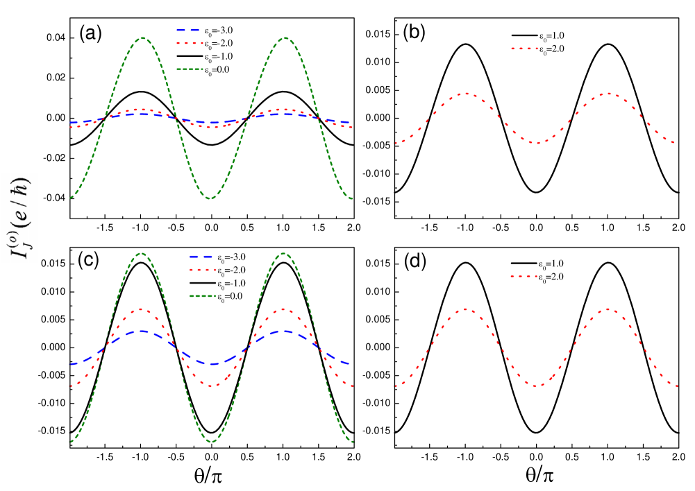
In Fig.2, we investigate the odd-FP Josephson current in Case I, and plot its spectra as a function of Josephson phase difference. As for the QD level and intradot Coulomb strength, we change $\varepsilon_{0}$ from $-3.0$ to $2.0$ in which $U$ is taken to be $0.0$ and $2.0$, respectively. In this figure, we find that despite the change of $\varepsilon_{0}$ and $U$, the leading oscillation property of the Josephson current is fixed. Namely, it reaches the maximum at the point $\theta=n\pi$ with its profile as $I^{(o)}_{J}\sim-\cos\theta$. However, the roles of QD level and Coulomb strength can also be clearly observed. With the departure of the QD level from energy zero point, the current amplitude will be suppressed gradually. Such a result is relatively apparent in Fig.2(a)-(b) where reflects the case of the zero Coulomb interaction. This can be explained as the weakness of the quantum coherence when the QD level is away from energy zero point. The effect of Coulomb interaction is notable in the region of $\varepsilon_{0}$, where the QD level is occupied. It can be found that Coulomb interaction suppresses the current amplitude as well. This should be attributed to the destruction of the quantum coherence induced by the QD-level splitting ($\varepsilon_{0}\to\varepsilon_{0}$ and $\varepsilon_{0}+U$) in the presence of Coulomb interaction.

Refer to caption
Figure 4: Josephson currents in Case III. The relevant parameters are taken to be $t_{T}=0.1$ and $t_{S}=0.5$. In the case of $\Delta_{s}=1.0$, the current amplitude $J$ will be equal to be $0.04$.
Refer to caption
Figure 5: (a)-(b) Geometries of the Josephson junction in Case I, Case II, and Case III in the Nambu representation, respectively.

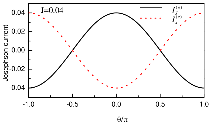
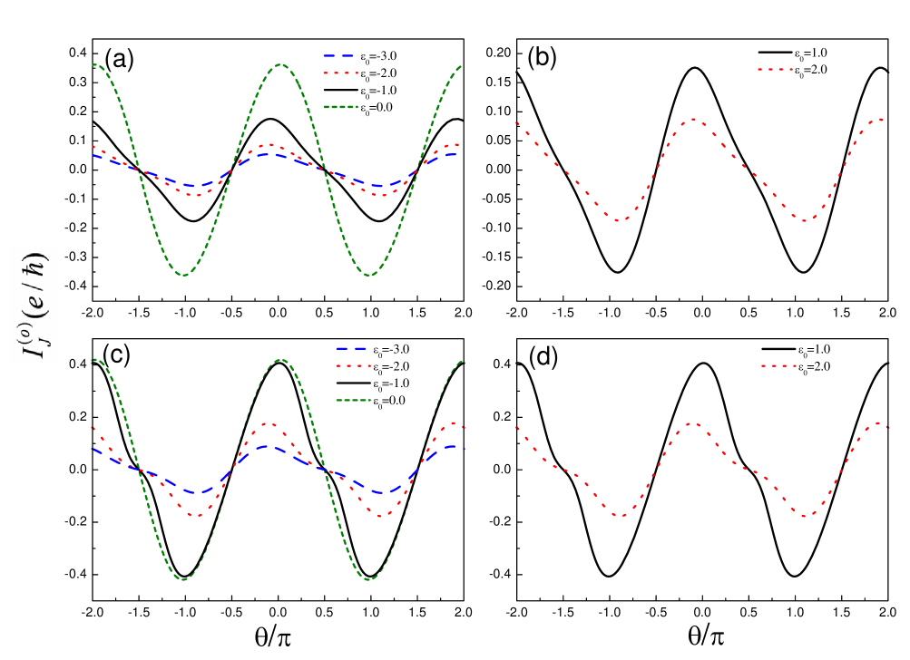
According to the discussion about Case II in the second part of Sec.II, when $t_{S}$ gets close to $t_{T}$, the $s$-wave superconductor should not be viewed as perturbation. It is natural to think that the Josephson current in such a case will show new properties. Next, we would like to increase the coupling strength between the QD and $s$-wave superconductor to discuss the change of Josephson effect. The numerical results are shown in Fig.3 where the $t_{T}=t_{S}=0.5$. In this figure, we see that in such a case, the current properties are completely different from those in Case I. Firstly, the current amplitude is efficiently enhanced by the increase of $t_{S}$. Secondly, the current direction is completely reversed and its profile is deviated from $I_{J}^{(o)}\sim\cos\theta$. If the coupling between the QD and $s$-wave superconductor further increases, the QD will be submerged in the $s$-wave superconductor. Consider the extreme case of the weak-coupling limit (i.e., Case III), the perturbation method can also be employed to evaluate the Josephson current, as displayed in the third part in Sec.II. It clearly shows that in such a case, the Majorana doublet couples weakly to the composite $s$-wave superconductor. Consequently, $I_{J}^{(o/e)}$ follow the relationship that $I_{J}^{(o/e)}=\pm J\cos\theta$ and their properties are clearly shown [See the results in Fig.4].

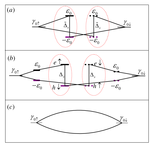
In view of the current results in Case I, Case II, and Case III, one can observe that at the case of $t_{T}\gg t_{S}$ (i.e., Case I), the current oscillation manner is opposite to that in the other two cases. In order to clarify the change of Josephson current from Case I to Case III, we present the geometries of these three cases in the Nambu representation, as shown in Fig.5. In Fig.5(a)-(c), we notice that the finite coupling between the two MBSs of Majorana doublet, despite the direct or indirect coupling, give rise to the occurrence of anomalous Josephson effect. On the other hand, the coupling strength between the QD and $s$-wave superconductor plays the role in altering the inter-MBS coupling property, leading to the change of the current oscillation manner. In the case of $t_{T}\ll t_{S}$, the MBSs couple directly to each other with a constant coupling parameter. In such case, the current direction is only dependent on the FP of the Majorana doublet with $I_{J}=[{e\over\hbar}]{\cal P}J\cos\theta$. In the other case where $t_{T}\gg t_{S}$, the coupling between the QD and Majorana doublet induces the indirect inter-MBS coupling, as shown in Fig.5(a). With respect to the inter-MBS coupling in these two cases, we find that in the former case, the MBSs couple to each other via a nonresonant Andreev reflection process, whereas in the latter case, one bound state is involved in the Andreev reflection process. It is well known that the quasi-particle phase will undergo a $\pi$-phase shift due to the presence of one bound state in the Andreev reflection process. Accordingly, for the case of identical FP, the current oscillations in Case I and Case III are opposite to each other. By the same token, we can easily see that in Case I and Case II, the oscillation manners of the Josephson current are opposite to each other, since an additional bound state is presented in the Andreev reflection process in Case II. Up to now, we have known the reason that in the considered junction, the current in the case of $t_{T}\gg t_{S}$ is different from that in the other cases. Also, note that in such a structure, the role of the $s$-wave superconductor is to provide a channel for the coupling between the MBSs in the Kramers doublet and the QD is to change the channel property. For this reason, the change of $\varepsilon_{0}$ and $U$ cannot induce any phase transition behaviors for the Josephson effect.

V Summary

In summary, in this work we have discussed the Josephson effects in the junction formed by a one dimensional DIII-class TS and a $s$-wave superconductor, by embedding a QD in such a junction. Via considering three QD-superconductor coupling manners, we have presented a comprehensive analysis about the Josephson effect in this system. As a consequence, it has been found that the Josephson current oscillates in $2\pi$ period. However, the presence of Majorana doublet in the DIII-class TS renders the Josephson current finite in the case of zero phase difference between the superconductors. With respect to the current direction, it is not only related to the FP of this junction but also depends on the coupling strength between the QD and $s$-wave superconductor. When the coupling between the QD and $s$-wave superconductor decreases to its weak limit, the direction of the Josephson current will have an opportunity to reverse. Via analyzing the particle motion in this structure, the reason for such a result has been clarified, namely, the QD-superconductor coupling manner can alter the property of the Andreev reflection between the MBSs in the Majorana doublet. It can be believed that this work be helpful for understanding the transport properties of the DIII-class TS.

Appendix

According to the Hamiltonian in Eq.(67), the coupling strength between the Majorana doublet and the $s$-wave superconductor, i.e., $\tilde{\Gamma}_{\sigma}=\pi\sum_{k}|W_{k}|^{2}\rho_{\sigma}$, where $\rho_{\sigma}$ is the density of state in the $s$-wave superconductor. Via a straightforward derivation, one can get the result that $\tilde{\Gamma}_{\sigma}=-t_{T}^{2}{\rm Im}G^{r}_{d\sigma}$. $G^{r}_{d\sigma}$, defined by Gd​σr​(t)=βˆ’i​θ​(t)β€‹βŸ¨{dσ​(t),dσ†}⟩subscriptsuperscriptπΊπ‘Ÿπ‘‘πœŽπ‘‘π‘–πœƒπ‘‘delimited-⟨⟩subscriptπ‘‘πœŽπ‘‘superscriptsubscriptπ‘‘πœŽβ€ G^{r}_{d\sigma}(t)=-i\theta(t)\langle\{d_{\sigma}(t),d_{\sigma}^{\dagger}\}\rangle, is a retarded Green function of one QD coupled to a $s$-wave superconductor. By means of the nonequilibrium Green function technique, the matrix of the retarded Green function $\textbf{G}^{r}_{d}$ can be obtained, i.e.,

$\displaystyle[\textbf{G}^{r}_{d}]^{-1}$ $\displaystyle=$ [(Ο‰βˆ’Ξ΅0)​Se↑+i​Γ0​ρ000βˆ’i​Δsω​Γ0​ρ00(Ο‰βˆ’Ξ΅0)​Se↓+i​Γ0​ρ0βˆ’i​Δsω​Γ0​ρ000βˆ’i​Δsω​Γ0​ρ0(Ο‰+Ξ΅0)​Sh↑+i​Γ0​ρ00βˆ’i​Δsω​Γ0​ρ000(Ο‰+Ξ΅0)​Sh↓+i​Γ0​ρ0],delimited-[]πœ”subscriptπœ€0subscript𝑆↑𝑒absent𝑖subscriptΞ“0subscript𝜌000𝑖subscriptΞ”π‘ πœ”subscriptΞ“0subscript𝜌00πœ”subscriptπœ€0subscript𝑆↓𝑒absent𝑖subscriptΞ“0subscript𝜌0𝑖subscriptΞ”π‘ πœ”subscriptΞ“0subscript𝜌000𝑖subscriptΞ”π‘ πœ”subscriptΞ“0subscript𝜌0πœ”subscriptπœ€0subscriptπ‘†β†‘β„Žabsent𝑖subscriptΞ“0subscript𝜌00𝑖subscriptΞ”π‘ πœ”subscriptΞ“0subscript𝜌000πœ”subscriptπœ€0subscriptπ‘†β†“β„Žabsent𝑖subscriptΞ“0subscript𝜌0\displaystyle\left[\begin{array}[]{cccc}(\omega-\varepsilon_{0})S_{e\uparrow}+i\Gamma_{0}\rho_{0}&0&0&-i{\Delta_{s}\over\omega}\Gamma_{0}\rho_{0}\\ 0&(\omega-\varepsilon_{0})S_{e\downarrow}+i\Gamma_{0}\rho_{0}&-i{\Delta_{s}\over\omega}\Gamma_{0}\rho_{0}&0\\ 0&-i{\Delta_{s}\over\omega}\Gamma_{0}\rho_{0}&(\omega+\varepsilon_{0})S_{h\uparrow}+i\Gamma_{0}\rho_{0}&0\\ -i{\Delta_{s}\over\omega}\Gamma_{0}\rho_{0}&0&0&(\omega+\varepsilon_{0})S_{h\downarrow}+i\Gamma_{0}\rho_{0}\\ \end{array}\right], (75)

where $\Gamma_{0}=\pi\sum_{k}|V_{kS}|^{2}\delta(\omega-\xi_{k})$ and $\rho_{0}={|\omega|\over\sqrt{\omega^{2}-\Delta_{s}^{2}}}$. $S_{e(h)\sigma}={\omega\pm\varepsilon_{0}\pm U\over\omega\pm\varepsilon_{0}\pm U\mp U\langle n_{\bar{\sigma}}\rangle}$ is the effect of the electron interaction within the Hubbard-I approximation and $\langle n_{\bar{\sigma}}\rangle$ is the average electron occupation number. In the absence of magnetic factors, such a system is spin-degenerated, hence $\textbf{G}^{r}_{d}$ can be simplified to be $2\times 2$ matrix, i.e.,

Gdr=[(Ο‰βˆ’Ξ΅0)​Se+i​Γ0​ρ0βˆ’i​Δsω​Γ0​ρ0βˆ’i​Δsω​Γ0​ρ0(Ο‰+Ξ΅0)​Sh+i​Γ0​ρ0]βˆ’1.subscriptsuperscriptGπ‘Ÿπ‘‘superscriptdelimited-[]πœ”subscriptπœ€0subscript𝑆𝑒𝑖subscriptΞ“0subscript𝜌0𝑖subscriptΞ”π‘ πœ”subscriptΞ“0subscript𝜌0missing-subexpressionmissing-subexpression𝑖subscriptΞ”π‘ πœ”subscriptΞ“0subscript𝜌0πœ”subscriptπœ€0subscriptπ‘†β„Žπ‘–subscriptΞ“0subscript𝜌0missing-subexpressionmissing-subexpression1\displaystyle\textbf{G}^{r}_{d}=\left[\begin{array}[]{cccc}(\omega-\varepsilon_{0})S_{e}+i\Gamma_{0}\rho_{0}&-i{\Delta_{s}\over\omega}\Gamma_{0}\rho_{0}\\ -i{\Delta_{s}\over\omega}\Gamma_{0}\rho_{0}&(\omega+\varepsilon_{0})S_{h}+i\Gamma_{0}\rho_{0}\\ \end{array}\right]^{-1}. (78)

In the limit of strong QD-superconductor coupling, the influence of $\omega$ and $\varepsilon_{0}$ will be submerged, and $G^{r}_{d\sigma}$ can be approximated as $-i{\rho_{0}/\Gamma_{0}}$, thus $\tilde{\Gamma}_{\sigma}\approx{t_{T}^{2}\rho_{0}/\Gamma_{0}}$. With the increment of $t_{S}$, $\Gamma_{0}$ will increase. This surely leads to the decrease of $\tilde{\Gamma}_{\sigma}$.

References

  • (1) M. Z. Hasan and C. L. Kane, Rev. Mod. Phys. 82, 3045(2010); X. L. Qi and S. C. Zhang, Rev. Mod. Phys. 83, 1057 (2011).
  • (2) C. Nayak, S. H. Simon, A. Stern, M. Freedman, S. Das Sarma, Rev. Mod. Phys. 80, 1083 (2008).
  • (3) F. Zhang, C. L. Kane, and E. J. Mele, Phys. Rev. Lett. 111, 056403 (2013).
  • (4) F. Hassler, A. R. Akhmerov, C. Y. Hou, and C. W. J. Beenakker, New J. Phys. 12, 125002 (2010); K. Flensberg, Phys. Rev. B 82, 180516(R) (2010).
  • (5) L. Fu and C. L. Kane, Phys. Rev. Lett. 100, 096407 (2008); E. J. H. Lee, X. Jiang, R. Aguado, G. Katsaros, C. M. Lieber, and S. De Franceschi, Phys. Rev. Lett. 109, 186802 (2012).
  • (6) B. van Heck, F. Hassler, A. R. Akhmerov, and C. W. J. Beenakker, Phys. Rev. B 84, 180502(R)(2011); P. Lucignano, F. Tafuri, and A. Tagliacozzo, Phys. Rev. B 88, 184512 (2013).
  • (7) D. Pekker, C. Y. Hou, V. E. Manucharyan, and E. Demler, Phys. Rev. Lett. 111, 107007 (2013); L. Jiang, D. Pekker, J. Alicea, G. Refael, Y. Oreg, and F. von Oppen, Phys. Rev. Lett. 107, 236401 (2011).
  • (8) P. A. Ioselevich and M. V. FeigeΕ‚man, Phys. Rev. Lett. 106, 077003 (2011).
  • (9) P. San-Jose, E. Prada, and R. Aguado, Phys. Rev. Lett. 108, 257001 (2012); R. M. Lutchyn, J. D. Sau, and S. Das Sarma, Phys. Rev. Lett. 105, 077001 (2010).
  • (10) A. P. Schnyder, S. Ryu, A. Furusaki, and A. W. W. Ludwig, Phys. Rev. B 78, 195125 (2008).
  • (11) X. L. Qi, T. L. Hughes, S. Raghu, and S.-C. Zhang, Phys. Rev. Lett. 102, 187001 (2009).
  • (12) J. C. Y. Teo and C. L. Kane, Phys. Rev. B 82, 115120 (2010).
  • (13) A. P. Schnyder, P.M. R. Brydon, D. Manske, and C. Timm, Phys. Rev. B 82, 184508 (2010).
  • (14) C. W. J. Beenakker, J. P. Dahlhaus, M. Wimmer, and A. R. Akhmerov, Phys. Rev. B 83, 085413 (2011).
  • (15) S. Deng, L. Viola, and G. Ortiz, Phys. Rev. Lett. 108, 036803 (2012).
  • (16) S. Nakosai, Y. Tanaka, and N. Nagaosa, Phys. Rev. Lett. 108, 147003 (2012).
  • (17) C. L. M. Wong and K. T. Law, Phys. Rev. B 86, 184516 (2012).
  • (18) F. Zhang, C. L. Kane, and E. J. Mele, Phys. Rev. Lett. 111, 056402 (2013).
  • (19) S. Nakosai, J. C. Budich, Y. Tanaka, B. Trauzettel, and N. Nagaosa, Phys. Rev. Lett. 110, 117002 (2013).
  • (20) A. Keselman, L. Fu, A. Stern, and E. Berg, Phys. Rev. Lett. 111, 116402 (2013).
  • (21) E. Gaidamauskas, J. Paaske, and K. Flensberg, Phys. Rev. Lett. 112, 126402 (2014).
  • (22) A. Haim, A. Keselman, E. Berg, and Y. Oreg, Phys. Rev. B 89, 220504(R) (2014).
  • (23) F. Zhang and C. L. Kane, Phys. Rev. B 90, 020501(R) (2014).
  • (24) E. Dumitrescu, J. D. Sau, and S. Tewari, arXiv:1310.7938.
  • (25) J. Klinovaja and D. Loss, Phys. Rev. B 90, 045118 (2014).
  • (26) S. B. Chung, J. Horowitz, and X. L. Qi, Phys. Rev. B 88, 214514 (2013).
  • (27) X. J. Liu, C. L. M. Wong, and K. T. Law, Phys. Rev. X 4, 021018 (2014).
  • (28) W. J. Gong, Z. Gao, W. F. Shan, and G. Y. Yi, arXiv:1501.02529.
  • (29) R. Allub and C. R. Proetto, Phys. Rev. B 62, 10923 (2000); E. Vecino, A. MartΓ­n-Rodero, and A. Levy Yeyati, Phys. Rev. B 68, 035105 (2003).
  • (30) A. A. Zyuzin, D. Rainis, J. Klinovaja, and D. Loss, Phys. Rev. Lett. 111, 056802 (2013).