Partial Network Alignment with Anchor Meta Path and Truncated Generic Stable Matching

Abstract

To enjoy more social network services, users nowadays are usually involved in multiple online social networks simultaneously. The shared users between different networks are called anchor users, while the remaining unshared users are named as non-anchor users. Connections between accounts of anchor users in different networks are defined as anchor links and networks partially aligned by anchor links can be represented as partially aligned networks. In this paper, we want to predict anchor links between partially aligned social networks, which is formally defined as the partial network alignment problem. The partial network alignment problem is very difficult to solve because of the following two challenges: (1) the lack of general features for anchor links, and (2) the “$one-to-one_{\leq}$” (one to at most one) constraint on anchor links. To address these two challenges, a new method PNA (Partial Network Aligner) is proposed in this paper. PNA (1) extracts a set of explicit anchor adjacency features and latent topological features for anchor links based on the anchor meta path concept and tensor decomposition techniques, and (2) utilizes the generic stable matching to identify the non-anchor users to prune the redundant anchor links attached to them. Extensive experiments conducted on two real-world partially aligned social networks demonstrate that PNA can solve the partial network alignment problem very well and outperform all the other comparison methods with significant advantages.

I Introduction

In recent years, online social networks providing various featured services have become an essential part in our lives. To enjoy more social network services, users nowadays are usually involved in multiple online social networks simultaneously [14, 36, 37, 42] and there can be significant overlaps of users shared by different networks. As pointed out in [6], by the end of 2013, $42\%$ of online adults are using multiple social sites at the same time. For example, $93\%$ of Instagram users are involved in Facebook concurrently and 53% Twitter users are using Instagram as well [19]. Formally, the common users involved in different networks simultaneously are named as the “anchor users” [14], while the remaining unshared users are called the “non-anchor users” [42]. The connections between accounts of anchor users in different networks are defined as the “anchor links” [14] and networks partially aligned by anchor links can be represented as “partially aligned networks” [37].

Problem Studied: In this paper, we want to predict the anchor links across partially aligned networks, which is formally defined as the “partial network alignment” problem.

Partial network alignment problem is very important for social networks and can be the prerequisite for many real-world social applications, e.g., link prediction and recommendations [36, 37, 42, 40], community detection [12, 39, 41] and information diffusion [35]. Identifying accounts of anchor users across networks provides the opportunity to compose a more complete social graph with users’ information in all the networks they are involved in. Information in the complete social graph is helpful for a better understanding of users’ social behavior in online social networks [14, 41, 35]. In addition, via the predicted anchor links, cross-platform information exchange enables new social networks to start their services based on the rich data available in other developed networks. The information transferred from developed networks can help emerging networks [37, 39] to overcome the information shortage problem promisingly [36, 37, 39].

What’s more, the partial network alignment problem is a novel problem and different from existing link prediction works, like (1) traditional intra-network link prediction problems [26, 27], which mainly focus on predicting links in one single social network, (2) inter-network link transfer problems [37], which can predict links in one single network with information from multiple aligned networks, and (3) inferring anchor links across fully aligned networks [14], which aims at predicting anchor links across fully aligned networks.

The inferring anchor links across fully aligned networks problem [14] also studies the anchor link prediction problem. However, both the problem setting and method proposed to address the “network alignment” problem between two fully aligned networks in [14] are very ad hoc and have many disadvantages. First of all, the full alignment assumption of social networks proposed in [14] is too strong as fully aligned networks can hardly exist in the real world [42]. Secondly, the features extracted for anchor links in [14] are proposed for Foursquare and Twitter specifically, which can be hard to get generalized to other networks. Thirdly, the classification based link prediction algorithm used in [14] can suffer from the class imbalance problem [16, 20]. The problem will be more serious when dealing with partially aligned networks. Finally, the matching algorithm proposed in [14] is designed specially for fully aligned networks and maps all users (including both anchor and non-anchor users) from one network to another network via the predicted anchor links, which will introduce a large number of non-existing anchor links when applied in the partial network alignment problem.

Totally different from the “inferring anchor links across fully aligned networks” problem [14], we study a more general network alignment problem in this paper. Firstly, networks studied in this paper are partially aligned [42], which contain large number of anchor and non-anchor users [42] at the same time. Secondly, networks studied are not confined to Foursquare and Twitter social networks. A minor revision of the “partial network alignment” problem can be mapped to many other existing tough problems, e.g., large biology network alignment [1], entity resolution in database integration [2], ontology matching [7], and various types of entity matching in online social networks [22]. Thirdly, the class imbalance problem will be addressed via link sampling effectively in the paper. Finally, the constraint on anchor links is “$one-to-one_{\leq}$” (i.e., each user in one network can be mapped to at most one user in another network). Across partially aligned networks, only anchor users can be connected by anchor links. Identifying the non-anchor users from networks and pruning all the predicted potential anchor links connected to them is a novel yet challenging problem. The “$one-to-one_{\leq}$” constraint on anchor links can distinguish the “partial network alignment” problem from most existing link prediction problems. For example, in traditional link prediction and link transfer problems [26, 27, 37], the constraint on links is “many-to-many”, while in the “anchor link inference” problem [14] across fully aligned networks, the constraint on anchor links is strict “one-to-one”.

To solve the “partial network alignment” problem, a new method, PNA (Partial Network Aligner), is proposed in this paper. PNA exploits the concept of anchor meta paths [42, 26] and utilizes the tensor decomposition [21, 13] technique to obtain a set of explicit anchor adjacency features and latent topological features. In addition, PNA generalizes the traditional stable matching to support partially aligned network through self-matching and partial stable matching and introduces the a novel matching method, generic stable matching, in this paper.

The rest of this paper is organized as follows. In Section II, we will give the definition of some important concepts and formulate the partial network alignment problem. PNA method will be introduces in Sections III-IV. Section V is about the experiments. Related works will be given in Section VI. Finally, we conclude the paper in Section VII.

II Problem Formulation

Before introducing the method PNA, we will first define some important concepts and formulate the partial network alignment problem in this section.

II-A Terminology Definition

Definition 1 (Heterogeneous Social Networks): A heterogeneous social network can be represented as $G=(\mathcal{V},\mathcal{E})$, where $\mathcal{V}=\bigcup_{i}\mathcal{V}_{i}$ contains the sets about various kinds of nodes, while $\mathcal{E}=\bigcup_{j}\mathcal{E}_{j}$ is the set of different types of links among nodes in $\mathcal{V}$.

Definition 2 (Aligned Heterogeneous Social Networks): Social networks that share common users are defined as the aligned heterogeneous social networks, which can be represented as $\mathcal{G}=(G_{set},A_{set})$, where $G_{set}=(G^{(1)},G^{(2)},\cdots,G^{(n)})$ is the set of $n$ different heterogeneous social networks and $A_{set}=(\mathcal{A}^{(1,2)},\mathcal{A}^{(1,3)},\cdots,\mathcal{A}^{((n-1),n)})$ is the sets of undirected anchor links between networks in $G_{set}$.

Definition 3 (Anchor Link): Given two social networks $G^{(i)}$ and $G^{(j)}$, link $(u^{(i)},v^{(j)})$ is an anchor link between $G^{(i)}$ and $G^{(j)}$ iff ($u^{(i)}\in\mathcal{U}^{(i)}$) $\land$ ($v^{(j)}\in\mathcal{U}^{(j)}$) $\land$ ($u^{(i)}$ and $v^{(j)}$ are accounts of the same user), where $\mathcal{U}^{(i)}$ and $\mathcal{U}^{(j)}$ are the user sets of $G^{(i)}$ and $G^{(j)}$ respectively.

Definition 4 (Anchor Users and Non-anchor Users): Users who are involved in two social networks, e.g., $G^{(i)}$ and $G^{(j)}$, simultaneously are defined as the anchor users between $G^{(i)}$ and $G^{(j)}$. Anchor users in $G^{(i)}$ between $G^{(i)}$ and $G^{(j)}$ can be represented as $\mathcal{U}^{(i)}_{\mathcal{A}^{(i,j)}}=\{u^{(i)}|u^{(i)}\in\mathcal{U}^{(i)},\exists v^{(j)}\in\mathcal{U}^{(j)},\mbox{ and }\\ (u^{(i)},v^{(j)})\in\mathcal{A}^{(i,j)}\}$. Meanwhile, the non-anchor user in $G^{(i)}$ between $G^{(i)}$ and $G^{(j)}$ are those who are involved in $G^{(i)}$ only and can be represented as $\mathcal{U}^{(i)}_{-\mathcal{A}^{(i,j)}}=\mathcal{U}^{(i)}-\mathcal{U}^{(i)}_{\mathcal{A}^{(i,j)}}$. Similarly, the anchor users and non-anchor users in $G^{(j)}$ between $G^{(j)}$ and $G^{(i)}$ can be defined as $\mathcal{U}^{(j)}_{\mathcal{A}^{(i,j)}}$ and $\mathcal{U}^{(j)}_{-\mathcal{A}^{(i,j)}}$ respectively.

Definition 5 (Full Alignment, Partial Alignment and Isolated): Given two social networks $G^{(i)}$ and $G^{(j)}$, if users in both $G^{(i)}$ and $G^{(j)}$ are all anchor users, i.e., $\mathcal{U}^{(i)}=\mathcal{U}^{(i)}_{\mathcal{A}^{(i,j)}}$ and $\mathcal{U}^{(j)}=\mathcal{U}^{(j)}_{\mathcal{A}^{(i,j)}}$, then $G^{(i)}$ and $G^{(j)}$ are fully aligned; if users in both of these two networks are all non-anchor users, i.e., $\mathcal{U}^{(i)}=\mathcal{U}^{(i)}_{-\mathcal{A}^{(i,j)}}$ and $\mathcal{U}^{(j)}=\mathcal{U}^{(j)}_{-\mathcal{A}^{(i,j)}}$, then these two networks are isolated; otherwise, they are partially aligned.

Definition 6 (Bridge Nodes): Besides users, many other kinds of nodes can be shared between different networks, which are defined as the bridge nodes in this paper. The bridge nodes shared between $G^{(i)}$ and $G^{(j)}$ can be represented as $\mathcal{B}^{(i,j)}=\{v|(v\in(\mathcal{V}^{(i)}-\mathcal{U}^{(i)}))\land(v\in(\mathcal{V}^{(j)}-\mathcal{U}^{(j)}))\}$.

The social networks studied in this paper can be any partially aligned social networks and we use Foursquare, Twitter as a example to illustrate the studied problem and the proposed method. Users in both Foursquare and Twitter can make friends with other users, write posts, which can contain words, timestamps, and location checkins. In addition, users in Foursquare can also create lists of locations that they have visited/want to visit in the future. As a result, Foursquare and Twitter can be represented as heterogeneous social network $G=(\mathcal{V},\mathcal{E})$. In Twitter $\mathcal{V}=\mathcal{U}\cup\mathcal{P}\cup\mathcal{W}\cup\mathcal{T}\cup\mathcal{L}$ and in Foursquare $\mathcal{V}=\mathcal{U}\cup\mathcal{P}\cup\mathcal{W}\cup\mathcal{T}\cup\mathcal{I}\cup\mathcal{L}$, where $\mathcal{U}$, $\mathcal{P}$, $\mathcal{W}$, $\mathcal{T}$, $\mathcal{I}$ and $\mathcal{L}$ are the nodes of users, posts, words, timestamps, lists and locations. While in Twitter, the heterogeneous link set $\mathcal{E}=\mathcal{E}_{u,u}\cup\mathcal{E}_{u,p}\cup\mathcal{E}_{p,w}\cup\mathcal{E}_{p,t}\cup\mathcal{E}_{p,l}$ and in Foursquare $\mathcal{E}=\mathcal{E}_{u,u}\cup\mathcal{E}_{u,p}\cup\mathcal{E}_{p,w}\cup\mathcal{E}_{p,t}\cup\mathcal{E}_{p,l}\cup\mathcal{E}_{u,i}\cup\mathcal{E}_{i,l}$. The bridge nodes shared between Foursquare and Twitter include the common locations, common words and common timestamps.

II-B Problem Statement

Definition 7 (Partial Network Alignment): For any two given partially aligned heterogeneous social networks, e.g., $\mathcal{G}=((G^{(i)},G^{(j)}),(\mathcal{A}^{(i,j)}))$, part of the known anchor links between $G^{(i)}$ and $G^{(j)}$ are represented as $\mathcal{A}^{(i,j)}$. Let $\mathcal{U}^{(i)}$, $\mathcal{U}^{(j)}$ be the user sets of $G^{(i)}$ and $G^{(j)}$ respectively, the set of other potential anchor links between $G^{(i)}$ and $G^{(j)}$ can be represented as $\mathcal{L}^{(i,j)}=\{(u^{(i)},v^{(j)})|(u^{(i)}\in\mathcal{U}^{(i)})\land(v^{(j)}\in\mathcal{U}^{(j)}\}-\mathcal{A}^{(i,j)}$. We solve the partial network alignment problem as a link classification problem, where existing and non-existing anchor links are labeled as “+1” and “-1” respectively. In this paper, we aim at building a model $\mathcal{M}$ with the existing anchor links $\mathcal{A}^{(i,j)}$, which will be applied to predict potential anchor links in $\mathcal{L}^{(i,j)}$. In model $\mathcal{M}$, we want to determine both labels and existence probabilities of anchor links in $\mathcal{L}^{(i,j)}$.

III Feature Extraction and Anchor Link Prediction

Supervised link prediction method has been widely used in research due to its excellent performance and the profound supervised learning theoretical basis. In supervised link prediction, links are labeled differently according to their physical meanings, e.g., existing vs non-existent [42], friends vs enemies [31], trust vs distrust [32], positive attitude vs negative attitude [33]. With information in the networks, a set of heterogeneous features can be extracted for links in the training set, which together with the labels are used to build the link prediction model $\mathcal{M}$.

In this section, we will introduce different categories of general features extracted for anchor links across partially aligned networks, which include a set of explicit anchor adjacency features based on anchor meta paths and the “latent topological feature vector” extracted via anchor adjacency tensor decomposition.

III-A Traditional Intra-Network Meta Path

Traditional meta paths are mainly defined based on the social network schema of one single network [26, 28].

Definition 8 (Social Network Schema): For a given network $G$, its schema is defined as $S_{G}=(\mathcal{T}_{G},\mathcal{R}_{G})$, where $\mathcal{T}_{G}$ and $\mathcal{R}_{G}$ are the sets of node types and link types in $G$ respectively.

Definition 9 (Meta Path): Based on the schema of network $G$, i.e., $S_{G}=(\mathcal{T}_{G},\mathcal{R}_{G})$, the traditional intra-network meta path in $G$ is defined as $\Phi=T_{1}\xrightarrow{R_{1}}T_{2}\xrightarrow{R_{2}}\cdots\xrightarrow{R_{k-1}}T_{k}$, where $T_{i}\in\mathcal{T}_{G},i\in\{1,2,\cdots,k\}$ and $R_{j}\in\mathcal{R}_{G},j\in\{1,2,\cdots,k-1\}$ [26, 28].

For example, according to the networks introduced in Section II, we can define the network schema of Twitter as $S_{G}=(\{User,Post,Word,Timestamp,List,Location\},\{Follow,\\ Write,Create,Contain,At,Checkin\})$. Based on the schema, “User - Location - User” is a meta path of length 2 connecting user nodes in the network via location node and path “Alice - San Jose - Bob” is an instance of such meta path in the network, where Alice, Bob and San Jose are the users and location in the network.

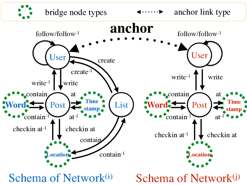
Figure 1: Schema of aligned heterogeneous network.

III-B Inter-Network Anchor Meta Path

Traditional Intra-network meta paths defined based on one single network cannot be applied to address the inter-network partial network alignment problem directly. To overcome such a problem, in this subsection, we will define the concept of anchor meta paths and introduce a set of inter-network anchor meta paths [42] across partially aligned networks.

Definition 10 (Aligned Social Network Schema): Given the partially aligned networks: $\mathcal{G}=(G_{set},A_{set})$, let $S_{G^{(i)}}=(\mathcal{T}_{G^{(i)}},\mathcal{R}_{G^{(i)}})$ be the schema of network $G^{(i)}\in G_{set}$, the schema of partially aligned networks $\mathcal{G}$ can be defined as $S_{\mathcal{G}}=\left(\bigcup_{i}\mathcal{T}_{G^{(i)}},(\bigcup_{i}\mathcal{R}_{G^{(i)}})\cup\{Anchor\}\right)$, where $\{Anchor\}$ is the anchor link type.

An example of the schema about two partially aligned social networks, e.g., $G^{(i)}$ (e.g., Foursquare) and $G^{(j)}$ (e.g., Twitter), is shown in Figure 1, where the schema of these two aligned networks are connected by the anchor link type and the green dashed circles are the shared bridge nodes between $G^{(i)}$ and $G^{(j)}$.

Definition 11 (AMP: Anchor Meta Path): Based on the aligned social network schema, anchor meta paths connecting users across $\mathcal{G}$ is defined to be $\Psi=T_{1}\xrightarrow{R_{1}}T_{2}\xrightarrow{R_{2}}\cdots\xrightarrow{R_{k-1}}T_{k}$, where $T_{1}$ and $T_{k}$ are the “User” node type in two partially aligned social networks respectively. To differentiate the anchor link type from other link types in the anchor meta path, the direction of $R_{i}$ in $\Psi$ will be bidirectional if $R_{i}=Anchor,i\in\{1,2,\cdots,k-1\}$, i.e., $T_{i}\ext@arrow 9999{\arrowfill@\leftarrow\relbar\rightarrow}{}{R_{i}}T_{j}$.

Via the instances of anchor meta paths, users across aligned social networks can be extensively connected to each other. In the two partially aligned social networks (e.g., $\mathcal{G}=((G^{(i)},G^{(j)}),(\mathcal{A}^{(i,j)}))$) studied in this paper, various anchor meta paths from $G^{(i)}$ (i.e., Foursquare) and $G^{(j)}$ (i.e., Twitter) can be defined as follows:

• Common Out Neighbor Anchor Meta Path ($\Psi_{1}$): $User^{(i)}$ $\xrightarrow{follow}$ $User^{(i)}$ $\ext@arrow 9999{\arrowfill@\leftarrow\relbar\rightarrow}{}{Anchor}$ $User^{(j)}$ $\xleftarrow{follow}$ $User^{(j)}$ or “$\mathcal{U}^{(i)}\to\mathcal{U}^{(i)}\leftrightarrow\mathcal{U}^{(j)}\leftarrow\mathcal{U}^{(j)}$” for short.

• Common In Neighbor Anchor Meta Path ($\Psi_{2}$): $User^{(i)}$ $\xleftarrow{follow}$ $User^{(i)}$ $\ext@arrow 9999{\arrowfill@\leftarrow\relbar\rightarrow}{}{Anchor}$ $User^{(j)}$ $\xrightarrow{follow}$ $User^{(j)}$ or “$\mathcal{U}^{(i)}\leftarrow\mathcal{U}^{(i)}\leftrightarrow\mathcal{U}^{(j)}\to\mathcal{U}^{(j)}$” .

• Common Out In Neighbor Anchor Meta Path ($\Psi_{3}$): $User^{(i)}$ $\xrightarrow{follow}$ $User^{(i)}$ $\ext@arrow 9999{\arrowfill@\leftarrow\relbar\rightarrow}{}{Anchor}$ $User^{(j)}$ $\xrightarrow{follow}$ $User^{(j)}$ or “$\mathcal{U}^{(i)}\to\mathcal{U}^{(i)}\leftrightarrow\mathcal{U}^{(j)}\to\mathcal{U}^{(j)}$”.

• Common In Out Neighbor Anchor Meta Path ($\Psi_{4}$): $User^{(i)}$ $\xleftarrow{follow}$ $User^{(i)}$ $\ext@arrow 9999{\arrowfill@\leftarrow\relbar\rightarrow}{}{Anchor}$ $User^{(j)}$ $\xleftarrow{follow}$ $User^{(j)}$ or “$\mathcal{U}^{(i)}\leftarrow\mathcal{U}^{(i)}\leftrightarrow\mathcal{U}^{(j)}\leftarrow\mathcal{U}^{(j)}$”.

These above anchor meta paths are all defined based the “User” node type only across partially aligned social networks. Furthermore, there can exist many other anchor meta paths consisting of user node type and other bridge node types from Foursquare to Twitter, e.g., Location, Word and Timestamp.

• Common Location Checkin Anchor Meta Path 1 ($\Psi_{5}$): $User^{(i)}$ $\xrightarrow{write}$ $Post^{(i)}$ $\xrightarrow{checkin\ at}$ $Location$ $\xleftarrow{checkin\ at}$ $Post^{(j)}$ $\xleftarrow{write}$ $User^{(j)}$ or “$\mathcal{U}^{(i)}\to\mathcal{P}^{(i)}\to\mathcal{L}\leftarrow\mathcal{P}^{(j)}\leftarrow\mathcal{U}^{(j)}$”.

• Common Location Checkin Anchor Meta Path 2 ($\Psi_{6}$): $User^{(i)}$ $\xrightarrow{create}$ $List^{(i)}$ $\xrightarrow{contain}$ $Location$ $\xleftarrow{checkin\ at}$ $Post^{(j)}$ $\xleftarrow{write}$ $User^{(j)}$ or “$\mathcal{U}^{(i)}\to\mathcal{I}^{(i)}\to\mathcal{L}\leftarrow\mathcal{P}^{(j)}\leftarrow\mathcal{U}^{(j)}$”.

• Common Timestamps Anchor Meta Path ($\Psi_{7}$): $User^{(i)}$ $\xrightarrow{write}$ $Post^{(i)}$ $\xrightarrow{at}$ $Time$ $\xleftarrow{at}$ $Post^{(j)}$ $\xleftarrow{write}$ $User^{(j)}$ or “$\mathcal{U}^{(i)}\to\mathcal{P}^{(i)}\to\mathcal{T}\leftarrow\mathcal{P}^{(j)}\leftarrow\mathcal{U}^{(j)}$”.

• Common Word Usage Anchor Meta Path ($\Psi_{8}$): $User^{(i)}$ $\xrightarrow{write}$ $Post^{(i)}$ $\xrightarrow{contain}$ $Word$ $\xleftarrow{contain}$ $Post^{(j)}$ $\xleftarrow{write}$ $User^{(j)}$ or “$\mathcal{U}^{(i)}\to\mathcal{P}^{(i)}\to\mathcal{W}\leftarrow\mathcal{P}^{(j)}\leftarrow\mathcal{U}^{(j)}$”.

III-C Explicit Anchor Adjacency Features

Based on the above defined anchor meta paths, different kinds of anchor meta path based adjacency relationship can be extracted from the network. In this paper, we define the new concepts of anchor adjacency score, anchor adjacency tensor and explicit anchor adjacency features to describe such relationships among users across partially aligned social networks.

Definition 12 (Anchor Meta Path Instance): Based on anchor meta path $\Psi=T_{1}\xrightarrow{R_{1}}T_{2}\xrightarrow{R_{2}}\cdots\xrightarrow{R_{k-1}}T_{k}$, path $\psi=n_{1}-n_{2}-\cdots-n_{k-1}-n_{k}$ is an instance of $\Psi$ iff $n_{i}$ is an instance of node type $T_{i}$, $i\in\{1,2,\cdots,k\}$ and $(n_{i},n_{i+1})$ is an instance of link type $R_{i}$, $\forall i\in\{1,2,\cdots,k-1\}$.

Definition 13 (AAS: Anchor Adjacency Score): The anchor adjacency score is quantified as the number of anchor meta path instances of various anchor meta paths connecting users across networks. The anchor adjacency score between $u^{(i)}\in\mathcal{U}^{(i)}$ and $v^{(j)}\in\mathcal{U}^{(j)}$ based on meta path $\Psi$ is defined as:

$$AAS_{\Psi}(u^{(i)},v^{(j)})=\left|\{\psi|(\psi\in\Psi)\land(u^{(i)}\in T_{1})\land(v^{(j)}\in T_{k})\}\right|,$$

where path $\psi$ starts and ends with node types $T_{1}$ and $T_{k}$ respectively and $\psi\in\Psi$ denotes that $\psi$ is a path instance of meta path $\Psi$.

The anchor adjacency scores among all users across partially aligned networks can be stored in the anchor adjacency matrix as follows.

Definition 14 (AAM: Anchor Adjacency Matrix): Given a certain anchor meta path, $\Psi$, the anchor adjacency matrix between $G^{i}$ and $G^{j}$ can be defined as $\mathbf{A}_{\Psi}\in\mathbb{N}^{|\mathcal{U}^{(i)}|\times|\mathcal{U}^{(j)}|}$ and $A(l,m)=AAS_{\Psi}(u_{l}^{(i)},u^{(j)}_{m}),u_{l}^{(i)}\in\mathcal{U}^{(i)},u^{(j)}_{m}\in\mathcal{U}^{(j)}.$

Multiple anchor adjacency matrix can be grouped together to form a high-order tensor. A tensor is a multidimensional array and an N-order tensor is an element of the tensor product of $N$ vector spaces, each of which can have its own coordinate system. As a result, an $1$-order tensor is a vector, a $2$-order tensor is a matrix and tensors of three or higher order are called the higher-order tensor [13, 21].

Definition 15 (AAT: Anchor Adjacency Tensor): Based on meta paths in $\{\Psi_{1},\Psi_{2},\cdots,\Psi_{8}\}$, we can obtain a set of anchor adjacency matrices between users in two partially aligned networks to be $\{\mathbf{A}_{\Psi_{1}},\mathbf{A}_{\Psi_{2}},\cdots,\mathbf{A}_{\Psi_{8}}\}$. With $\{\mathbf{A}_{\Psi_{1}},$ $\mathbf{A}_{\Psi_{2}},$ $\cdots,$ $\mathbf{A}_{\Psi_{8}}\}$, we can construct a 3-order anchor adjacency tensor $\mathcal{X}\in\mathbb{R}^{|\mathcal{U}^{(i)}|\times|\mathcal{U}^{(j)}|\times 8}$, where the $i_{th}$ layer of $\mathcal{X}$ is the anchor adjacency matrix based on anchor meta path $\Psi_{i}$, i.e., $\mathcal{X}(:,:,i)=\mathbf{A}_{\Psi_{i}},i\in\{1,2,\cdots,8\}$.

Based on the anchor adjacency tensor, a set of explicit anchor adjacency features can be extracted for anchor links across partially aligned social networks.

Definition 16 (EAAF: Explicit Anchor Adjacency Features): For a certain anchor link $(u^{(i)}_{l},u^{(j)}_{m})$, the explicit anchor adjacency feature vectors extracted based on the anchor adjacency tensor $\mathcal{X}$ can be represented as $\mathbf{x}=[x_{1},x_{2},\cdots,x_{8}]$ (i.e., the anchor adjacency scores between $u^{(i)}_{l}$ and $u^{(j)}_{m}$ based on $8$ different anchor meta paths), where $x_{k}=\mathcal{X}(l,m,k),k\in\{1,2,\cdots,8\}.$

III-D Latent Topological Feature Vectors Extraction

Explicit anchor adjacency features can express manifest properties of the connections across partially aligned networks and are the explicit topological features. Besides explicit topological connections, there can also exist some hidden common connection patterns [33] across partially aligned networks. In this paper, we also propose to extract the latent topological feature vectors from the anchor adjacency tensor.

As proposed in [13, 21], a higher-order tensor can be decomposed into a core tensor, e.g., $\mathcal{G}$, multiplied by a matrix along each mode, e.g., $\mathbf{A},\mathbf{B},\cdots,\mathbf{Z}$, with various tensor decomposition methods, e.g., Tucker decomposition [13]. For example, the 3-order anchor adjacency tensor $\mathcal{X}$ can be decomposed into three matrices $\mathbf{A}\in\mathbb{R}^{\mathcal{U}^{(i)}\times P}$, $\mathbf{B}\in\mathbb{R}^{\mathcal{U}^{(j)}\times Q}$ and $\mathbf{C}\in\mathbb{R}^{8\times R}$ and a core tensor $\mathcal{G}\in\mathbb{R}^{P\times Q\times R}$, where $P,Q,R$ are the number of columns of matrices $\mathbf{A},\mathbf{B},\mathbf{C}$ [13]:

$$\mathcal{X} =\sum_{p=1}^{P}\sum_{q=1}^{Q}\sum_{r=1}^{R}g_{pqr}\mathbf{a}_{p}\circ\mathbf{b}_{q}\circ\mathbf{c}_{r}=[\mathcal{G};\mathbf{A},\mathbf{B},\mathbf{C}],$$

where $\mathbf{a}_{p}\circ\mathbf{b}_{q}$ denotes the vector outer product of $\mathbf{a}_{p}$ and $\mathbf{b}_{q}$.

Each row of $\mathbf{A}$ and $\mathbf{B}$ represents a latent topological feature vector of users in $\mathcal{U}^{(i)}$ and $\mathcal{U}^{(j)}$ respectively [21]. Method HOSVD introduced in [13] is applied to achieve these decomposed matrices in this paper.

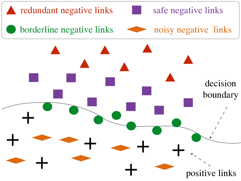
Figure 2: Instance distribution in feature space.

III-E Class Imbalance Link Prediction

Based on the extracted features, various supervised link prediction models [14, 37, 42] can be applied to infer the potential anchor links across networks. As proposed in [20, 16], conventional supervised link prediction methods [29], can suffer from the class imbalance problem a lot. To address the problem, two effective methods (down sampling [15] and over sampling [4]) are applied.

Down sampling methods aim at deleting the unreliable negative instances from the training set. In Figure 2, we show the distributions of training links in the feature space, where negative links can be divided into $4$ different categories [15]: (1) noisy links: links mixed in the positive links; (2) borderline links: links close to the decision boundary; (3) redundant links: links which are too far away from the decision boundary in the negative region; and (4) safe links: links which are helpful for determining the classification boundary.

Different heuristics have been proposed to remove the noisy instances and borderline instances, which are detrimental for the learning algorithms. In this paper, we will use the method called Tomek links proposed in [30, 15]. For any two given instances $\mathbf{x}_{1}$ and $\mathbf{x}_{2}$ of different labels, pair $(\mathbf{x}_{1},\mathbf{x}_{2})$ is called a tomek link if there exists no other instances, e.g., $\mathbf{z}$, such that $d(\mathbf{x}_{1},\mathbf{z})<d(\mathbf{x}_{1},\mathbf{x}_{2})$ and $d(\mathbf{x}_{2},\mathbf{z})<d(\mathbf{x}_{1},\mathbf{x}_{2})$. Examples that participate in Tomek links are either borderline or noisy instances [30, 15]. As to the redundant instances, they will not harm correct classifications as their existence will not change the classification boundary but they can lead to extra classification costs. To remove the redundant instances, we propose to create a consistent subset $\mathcal{C}$ of the training set, e.g., $\mathcal{S}$ [15]. Subset $\mathcal{C}$ is consistent with $\mathcal{S}$ if classifiers built with $\mathcal{C}$ can correctly classify instances in $\mathcal{S}$. Initially, $\mathcal{C}$ consists of all positive instances and one randomly selected negative instances. A classifier, e.g., $kNN$, built with $\mathcal{C}$ is applied to $\mathcal{S}$, where instances that are misclassified are added into $\mathcal{C}$. The final set $\mathcal{C}$ contains the safe links.

Another method to overcome the class imbalance problem is to over sample the minority class. Many over sampling methods have been proposed, e.g., over sampling with replacement, over sampling with “synthetic” instances [4]: the minority class is over sampled by introducing new “synthetic” examples along the line segment joining $m$ of the $k$ nearest minority class neighbors for each minority class instances. Parameter $k$ is usually set as $5$, while the value of $m$ can be determined according to the ratio to over sample the minority class. For example, if the minority class need to be over sampled $200\%$, then $m=2$. The instance to be created between a certain example $\mathbf{x}$ and one of its nearest neighbor $\mathbf{y}$ can be denoted as $\mathbf{x}+\mathbf{\theta}^{T}(\mathbf{x}-\mathbf{y})$, where $\mathbf{x}$ and $\mathbf{y}$ are the feature vectors of two instances and $\mathbf{\theta}^{T}$ is the transpose of a coefficient vector containing random numbers in range $[0,1]$.

IV Anchor Link Pruning with Generic Stable Matching

In this section, we will introduce the anchor link pruning methods in details, which include (1) candidate pre-pruning, (2) brief introduction to the traditional stable matching, and (3) the generic stable matching method proposed in this paper, which generalizes the concept of traditional stable matching through both self matching and partial stable matching.

IV-A Candidate Pre-Pruning

Across two partially aligned social networks, users in a certain network can have a large number of potential anchor link candidates in the other network, which can lead to great time and space costs in predicting the anchor links. The problem can be even worse when the networks are of large scales, e.g., containing million even billion users, which can make the partial network alignment problem unsolvable. To shrink size of the candidate set, we propose to conduct candidate pre-pruning of links in the test set with users’ profile information (e.g., names and hometown).

As shown in Figure 3, in the given input test set, users are extensively connected with all their potential partners in other networks via anchor links. For each users, we propose to prune their potential candidates according to the following heuristics:

• profile pre-pruning: users’ profile information shared across partially aligned social networks, e.g., Foursquare and Twitter, can include username and hometown [34]. Given an anchor link $(u^{(i)}_{l},u^{(j)}_{m})\in\mathcal{L}$, if the username and hometown of $u^{(i)}_{l}$ and $u^{(j)}_{m}$ are totally different, e.g., cosine similarity scores are $0$, then link $(u^{(i)}_{l},u^{(j)}_{m})$ will be pruned from test set $\mathcal{L}$.

• EAAF pruning: based on the explicit anchor adjacency tensor $\mathcal{X}$ extracted in Section III, for a given link $(u^{(i)}_{l},u^{(j)}_{m})\in\mathcal{L}$, if its extracted explicit anchor adjacency features are all $0$, i.e., $\mathcal{X}(l,m,x)=0,x\in\{1,2,\cdots,8\}$, then link $(u^{(i)}_{l},u^{(j)}_{m})$ will be pruned from test set $\mathcal{L}$.

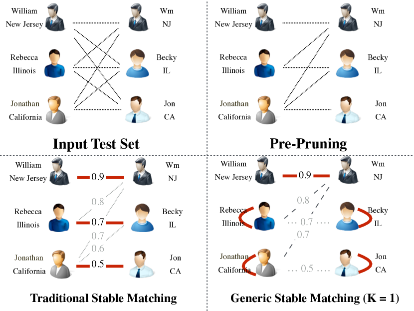
Figure 3: Partial network alignment with pruning.

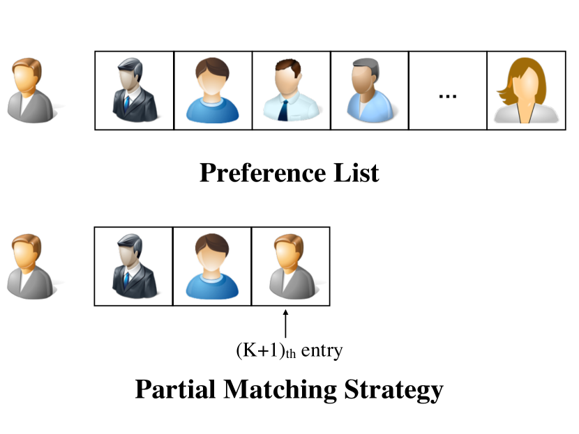
Figure 4: Example of partial matching strategy(K=2).

IV-B Traditional Stable Matching

Meanwhile, as proposed in [14], the one-to-one constraint of anchor links across fully aligned social networks can be met by pruning extra potential anchor link candidates with traditional stable matching. In this subsection, we will introduce the concept of traditional stable matching briefly.

Given the user sets $\mathcal{U}^{(1)}$ and $\mathcal{U}^{(2)}$ of two partially aligned social networks $G^{(1)}$ and $G^{(2)}$, each user in $\mathcal{U}^{(1)}$(or $\mathcal{U}^{(2)}$) has his preference over users in $\mathcal{U}^{(2)}$(or $\mathcal{U}^{(1)}$). Term $v_{j}P^{(1)}_{u_{i}}v_{k}$ is used to denote that $u_{i}\in\mathcal{U}^{(1)}$ prefers $v_{j}$ to $v_{k}$ for simplicity, where $v_{j},v_{k}\in\mathcal{U}^{(2)}$ and $P^{(1)}_{u_{i}}$ is the preference operator of ${u_{i}}\in\mathcal{U}^{(1)}$. Similarly, we can use term $u_{i}P^{(2)}_{v_{j}}u_{k}$ to denote that $v_{j}\in\mathcal{U}^{(2)}$ prefers $u_{i}$ to $u_{k}$ in $\mathcal{U}^{(1)}$ as well.

Definition 17 (Matching): Mapping $\mu:\mathcal{U}^{(1)}\cup\mathcal{U}^{(2)}\to\mathcal{U}^{(1)}\cup\mathcal{U}^{(2)}$ is defined to be a matching iff (1) $|\mu(u_{i})|=1,\forall u_{i}\in\mathcal{U}^{(1)}$ and $\mu(u_{i})\in\mathcal{U}^{(2)}$; (2) $|\mu(v_{j})|=1,\forall v_{j}\in\mathcal{U}^{(2)}$ and $\mu(v_{j})\in\mathcal{U}^{(1)}$; (3) $\mu(u_{i})=v_{j}$ iff $\mu(v_{j})=u_{i}$.

Definition 18 (Blocking Pair): A pair $(u_{i},v_{j})$ is a a blocking pair of matching $\mu$ if $u_{i}$ and $v_{j}$ prefers each other to their mapped partner, i.e., $(\mu(u_{i})\neq v_{j})\land(\mu(v_{j})\neq u_{i})$ and $(v_{j}P^{(1)}_{u_{i}}\mu(u_{i}))\land(u_{i}P^{(2)}_{v_{j}}\mu(v_{j}))$.

Definition 19 (Stable Matching): Given a matching $\mu$, $\mu$ is stable if there is no blocking pair in the matching results [5].

As introduced in [14], the stable matching can be obtained with the Gale-Shapley algorithm proposed in [9].

IV-C Generic Stable Matching

Stable matching based method proposed in [14] can only work well in fully aligned social networks. However, in the real world, few social networks are fully aligned and lots of users in social networks are involved in one network only, i.e., non-anchor users, and they should not be connected by any anchor links. However, traditional stable matching method cannot identify these non-anchor users and remove the predicted potential anchor links connected with them. To overcome such a problem, we will introduce the generic stable matching to identify the non-anchor users and prune the anchor link results to meet the $one-to-one_{\leq}$ constraint.

In PNA, we introduce a novel concept, self matching, which allows users to be mapped to themselves if they are discovered to be non-anchor users. In other words, we will identify the non-anchor users as those who are mapped to themselves in the final matching results.

Definition 20 (Self Matching): For the given two partially aligned networks $G^{(1)}$ and $G^{(2)}$, user $u_{i}\in\mathcal{U}^{(1)}$, can have his preference $P^{(1)}_{u_{i}}$ over users in $\mathcal{U}^{(2)}\cup\{u_{i}\}$ and $u_{i}$ preferring $u_{i}$ himself denotes that $u_{i}$ is an non-anchor user and prefers to stay unconnected, which is formally defined as self matching.

Users in one social network will be matched with either partners in other social networks or themselves according to their preference lists (i.e., from high preference scores to low preference scores). Only partners that users prefer over themselves will be accepted finally, otherwise users will be matched with themselves instead.

Definition 21 (Acceptable Partner): For a given matching $\mu:\mathcal{U}^{(1)}\cup\mathcal{U}^{(2)}\to\mathcal{U}^{(1)}\cup\mathcal{U}^{(2)}$, the mapped partner of users $u_{i}\in\mathcal{U}^{(1)}$, i.e., $\mu(u_{i})$, is acceptable to $u_{i}$ iff $\mu(u_{i})P^{(1)}_{u_{i}}u_{i}$.

To cut off the partners with very low preference scores, we propose the partial matching strategy to obtain the promising partners, who will participate in the matching finally.

Definition 22 (Partial Matching Strategy): The partial matching strategy of user $u_{i}\in\mathcal{U}^{(1)}$, i.e., $Q^{(1)}_{u_{i}}$, consists of the first $K$ the acceptable partners in $u_{i}$’s preference list $P^{(1)}_{u_{i}}$, which are in the same order as those in $P^{(1)}_{u_{i}}$, and $u_{i}$ in the $(K+1)_{th}$ entry of $Q^{(1)}_{u_{i}}$. Parameter $K$ is called the partial matching rate in this paper.

An example is given in Figure 4, where to get the top $2$ promising partners for the user, we place the user himself at the $3_{rd}$ cell in the preference list. All the remaining potential partners will be cut off and only the top $3$ users will participate in the final matching.

Based on the concepts of self matching and partial matching strategy, we define the concepts of partial stable matching and generic stable matching as follow.

Definition 23 (Partial Stable Matching): For a given matching $\mu$, $\mu$ is (1) rational if $\mu(u_{i})Q^{(1)}_{u_{i}}u_{i},\forall u_{i}\in\mathcal{U}^{(1)}$ and $\mu(v_{j})Q^{(2)}_{v_{j}}v_{j},\forall v_{j}\in\mathcal{U}^{(2)}$, (2) pairwise stable if there exist no blocking pairs in the matching results, and (3) stable if it is both rational and pairwise stable.

Definition 24 (Generic Stable Matching): For a given matching $\mu$, $\mu$ is a generic stable matching iff $\mu$ is a self matching or $\mu$ is a partial stable matching.

As example of generic stable matching is shown in the bottom two plots of Figure 3. Traditional stable matching can prune most non-existing anchor links and make sure the results can meet one-to-one constraint. However, it preserves the anchor links (Rebecca, Becky) and (Jonathan, Jon), which are connecting non-anchor users. In generic stable matching with parameter $K=1$, users will be either connected with their most preferred partner or stay unconnected. Users “William” and “Wm” are matched as link (William, Wm) has the highest score. “Rebecca” and “Jonathan” will prefer to stay unconnected as their most preferred partner “Wm” is connected with “William” already. Furthermore, “Becky” and “Jon” will stay unconnected as their most preferred partner “Rebecca” and “Jonathan” prefer to stay unconnected. In this way, generic stable matching can further prune the non-existing anchor links (Rebecca, Becky) and (Jonathan, Jon).

The truncated generic stable matching results can be achieved with the Generic Gale-Shapley algorithm as given in Algorithm 1.

Algorithm 1 Generic Gale-Shapley Algorithm

0:  user sets of aligned networks: $\mathcal{U}^{(1)}$ and $\mathcal{U}^{(2)}$.   classification results of potential anchor links in $\mathcal{L}$  known anchor links in $\mathcal{A}^{(1,2)}$  truncation rate $K$

0:  a set of inferred anchor links $\mathcal{L}^{\prime}$

1:  Initialize the preference lists of users in $\mathcal{U}^{(1)}$ and $\mathcal{U}^{(2)}$ with predicted existence probabilities of links in $\mathcal{L}$ and known anchor links in $\mathcal{A}^{(1,2)}$, whose existence probabilities are $1.0$

2:  construct the truncated strategies from the preference lists

3:  Initialize all users in $\mathcal{U}^{(1)}$ and $\mathcal{U}^{(2)}$ as free

4:  $\mathcal{L}^{\prime}=\emptyset$

5:  while $\exists$ free $u^{(1)}_{i}$ in $\mathcal{U}^{(1)}$ and $u^{(1)}_{i}$’s truncated strategy is non-empty do

6:     Remove the top-ranked account $u^{(2)}_{j}$ from $u^{(1)}_{i}$’s truncated strategy

7:     if $u^{(2)}_{j}$==$u^{(1)}_{i}$ then

8:        $\mathcal{L}^{\prime}=\mathcal{L}^{\prime}\cup\{(u^{(1)}_{i},u^{(1)}_{i})\}$

9:        Set $u^{(1)}_{i}$ as stay unconnected

10:     else

11:        if  $u^{(2)}_{j}$ is free then

12:           $\mathcal{L}^{\prime}=\mathcal{L}^{\prime}\cup\{(u^{(1)}_{i},u^{(2)}_{j})\}$

13:           Set $u^{(1)}_{i}$ and $u^{(2)}_{j}$ as occupied

14:        else

15:           $\exists u^{(1)}_{p}$ that $u^{(2)}_{j}$ is occupied with.

16:           if  $u^{(2)}_{j}$ prefers $u^{(1)}_{i}$ to $u^{(1)}_{p}$ then

17:              $\mathcal{L}^{\prime}=(\mathcal{L}^{\prime}-\{(u^{(1)}_{p},u^{(2)}_{j})\})\cup\{(u^{(1)}_{i},u^{(2)}_{j})\}$

18:              Set $u^{(1)}_{p}$ as free and $u^{(1)}_{i}$ as occupied

19:           end if

20:        end if

21:     end if

22:  end while

V Experiments

TABLE I: Properties of the Heterogeneous Networks

		network
	property	Twitter	Foursquare
# node	user	5,223	5,392
	tweet/tip	9,490,707	48,756
	location	297,182	38,921
# link	friend/follow	164,920	76,972
	write	9,490,707	48,756
	locate	615,515	48,756

To demonstrate the effectiveness of PNA in predicting anchor links for partially aligned heterogeneous social networks, we conduct extensive experiments on two real-world heterogeneous social networks: Foursquare and Twitter. This section includes three parts: (1) dataset description, (2) experiment settings, and (3) experiment results.

V-A Dataset Description

The datasets used in this paper include: Foursquare and Twitter, which were crawled during November 2012 [14, 36, 37, 42]. More detailed information about these two datasets is shown in Table I and in [14, 36, 37, 42]. The number of anchor links crawled between Foursquare and Twitter is $3,388$ and $62.83\%$ Foursquare users are anchor users.

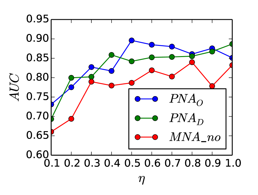
(a) AUC: alignment rate

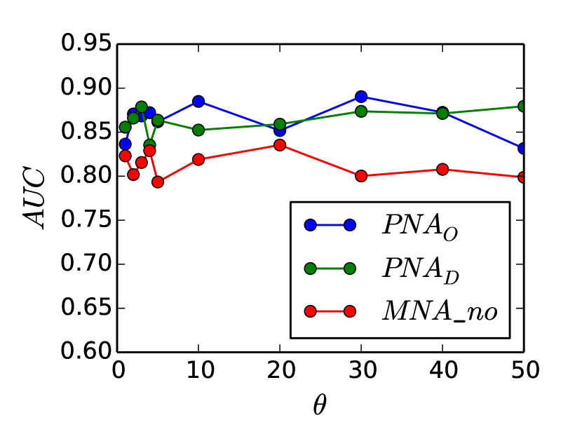
(b) AUC: negative positive rate

Figure 5: AUC of different class imbalance link prediction methods.

V-B Experiment Settings

In this part, we will talk about the experiment settings in details, which includes: (1) comparison methods, (2) evaluation methods, and (3) experiment setups.

V-B1 Comparison Methods

The comparison methods used in the experiments can be divided into the following $4$ categories:

Methods with Generic Stable Matching:

• PNAomg: PNAomg (PNA with Over sampling & Generic stable Matching) is the method proposed in this paper, which consists of two steps: (1) class imbalance link prediction with over sampling, and (2) candidate pruning with generic stable matching.

• PNAdmg: PNAdmg (PNA with Down sampling & Generic stable Matching) is another method proposed in this paper, which consists of two steps: (1) class imbalance link prediction with down sampling, and (2) candidate pruning with generic stable matching.

Methods with Traditional Stable Matching

• PNAom: PNAom (PNA with Over sampling & traditional stable Matching) is identical to PNAomg except that in the second step, PNAom applies the traditional stable matching [9, 14].

• PNAdm: PNAdm (PNA with Down sampling & traditional stable Matching) is identical to PNAdmg except that in the second step, PNAdm applies the traditional stable matching [9, 14].

Class Imbalance Anchor Link Prediction:

• PNAo: PNAo (PNA with Over sampling) is the link prediction method with over sampling to overcome the class imbalance problem and has no matching step.

• PNAd: PNAd (PNA with Down sampling) is the link prediction method with down sampling to overcome the class imbalance problem and has no matching step.

Existing Network Anchoring Methods

• Mna: Mna (Multi-Network Anchoring) is a two-phase method proposed in [14] which includes: (1) supervised link prediction without addressing class imbalance problem; (2) traditional stable matching [9, 14].

• Mna_no: Mna_no (Mna without one-to-one constraint) is the first step of Mna proposed in [14] which can predict anchor links without addressing the class imbalance problem and has no matching step.

V-B2 Evaluation Metrics

The output of different link prediction methods can be either predicted labels or confidence scores, which are evaluated by Accuracy, AUC, F1 in the experiments.

V-B3 Experiment Setups

In the experiment, initially, a fully aligned network containing $3000$ users in both Twitter and Foursquare is sampled from the datasets. All the existing anchor links are grouped into the positive link set and all the possible non-existing anchor links are used as the potential link set. Certain number of links are randomly sampled from the potential link set as the negative link set, which is controlled by parameter $\theta$. Parameter $\theta$ represents the $\frac{\#negative}{\#positive}$ rate, where $\theta=1$ denotes the class balance case, i.e., $\#positive$ equals to $\#negative$; $\theta=50$ represents that case that negative instance set is $50$ times as large as that of the positive instance set, i.e., $\#negative=50\times\#positive$. In the experiment, $\theta$ is chosen from $\{1,2,3,4,5,10,20,30,40,50\}$. Links in the positive and negative link sets are partitioned into two parts with 10-fold cross validation, where $9$ folds are used as the training set and $1$ fold is used as the test set. To simulate the partial alignment networks, certain positive links are randomly sampled from the positive training set as the final positive training set under the control of parameter $\eta$. $\eta$ is chosen from $\{0.1,0.2,\cdots,1.0\}$, where $\eta=0.1$ denotes that the networks are $10\%$ aligned and $\eta=1.0$ shows that the networks are fully aligned. With links in the positive training set, anchor adjacency tensor based features and the latent feature vectors are extracted from the network to build link prediction model $\mathcal{M}$. In building model $\mathcal{M}$, over sampling and under sampling techniques are applied and the sampling rate is determined by parameter $\sigma\in\{0.0,0.1,0.2,\cdots,1.0\}$, where $\sigma=0.3$ denotes that $0.3\times(\#negative-\#positive)$ negative links are randomly removed from the negative link set in under sampling; or $0.3\times(\#negative-\#positive)$ positive links are generated and added to the positive link set in over sampling. Before applying model $\mathcal{M}$ to the test set, pre-pruning process is conducted on the test set in advance. Based on the prediction results of model $\mathcal{M}$ on the test set, post-pruning with generic stable matching is applied to further prune the non-existent candidates to ensure that the final prediction results across the partially aligned networks can meet the $one-to-one_{\leq}$ constraint controlled by the partial matching parameter $K$.

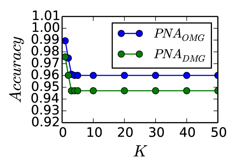
(a) Acc.@$\theta=5$, $\eta=0.4$

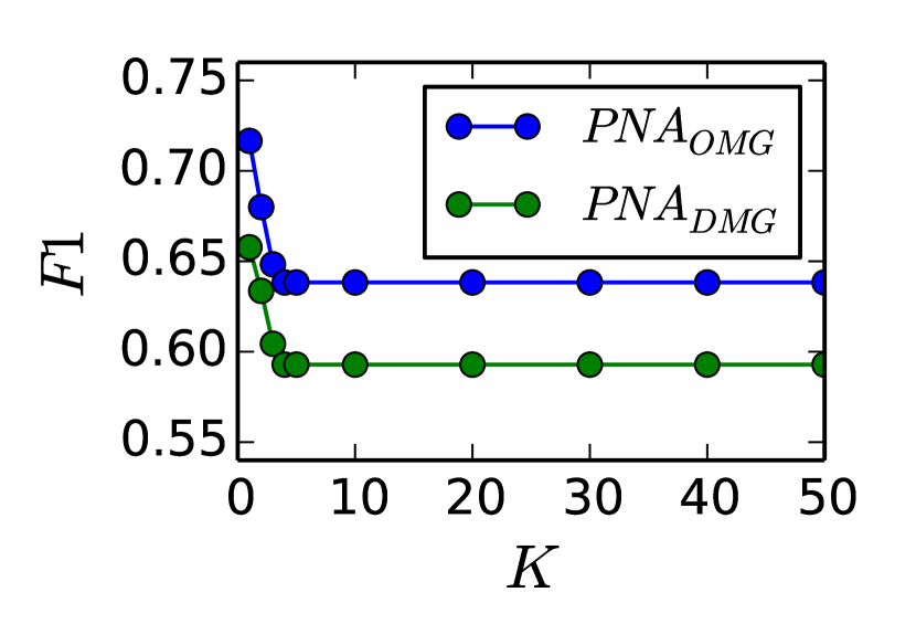
(b) F1@$\theta=5$, $\eta=0.4$

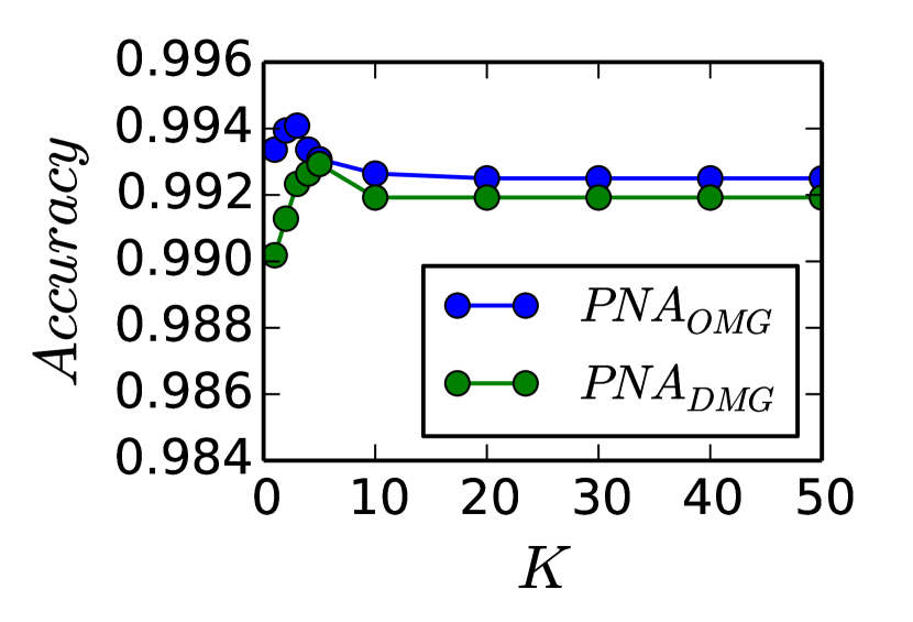
(c) Acc.@$\theta=50$, $\eta=0.9$

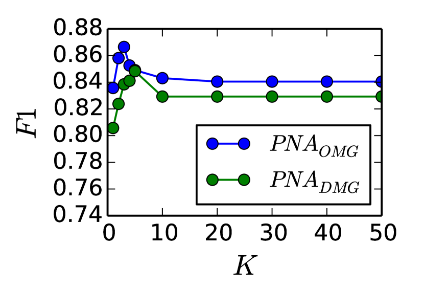
(d) F1@$\theta=50$, $\eta=0.9$

Figure 6: F1, Accuracy of PNAomg and PNAdmg with different partial matching rates.

V-C Experiment Results

In this part, we will give the experiment results of all these comparison methods in addressing the partial network alignment problem. This part includes (1) analysis of sampling methods in class imbalance link prediction; (2) performance comparison of different link prediction methods; and (3) parameter analysis.

V-C1 Analysis of Sampling Methods

To examine whether sampling methods can improve the prediction performance on the imbalanced classification problem or not, we also compare PNAo, PNAd with Mna_no and the results are given in Figure 5, where we fix $\theta$ as 10 but change $\eta$ with values in $\{0.1,0.2,\cdots,1.0\}$ and compare the AUC achieved by PNAo, PNAd and Mna_no. We can observe that the AUC values of all these three methods increases with the increase of $\eta$ but PNAo and PNAd perform consistently better than Mna_no. In Figure 5(b), we fix $\eta$ as $0.6$ but change $\theta$ with values in {1, 2, 3, 4, 5, 10, 20, 30, 40, 50} and compare the AUC of PNAo, PNAd and Mna_no. As shown in Figure 5(b), the performance of PNAo, PNAd and Mna_no can all varies slightly with $\theta$ changing from $1$ to $50$ and PNAo, PNAd can achieve better performance than Mna_no consistently.

V-C2 Comparison of Different Link Prediction Methods

Meanwhile, as generic stable matching based post pruning can only output the labels of potential anchor links in the test set, we also evaluate all these methods by comparing their Accuracy and F1 score Tables II-III. In Table II, we fix $\theta$ as $10$, $K$ as $5$ but change $\eta$ with values in $\{0.1,0.2,\cdots,1.0\}$. Table II has two parts. The upper part of Table II shows the Accuracy achieved by all the methods with various $\eta$, and the lower part shows the F1 score. Generally, the performance of all comparison methods rises as $\eta$ increases. In the upper part, methods PNAomg and PNAdmg can consistently perform better than all other comparison methods for different $\eta$. For example, when $\eta=0.5$, the Accuracy achieved by PNAomg is higher than PNAom by $3.45\%$, higher than Mna by $6.0\%$, higher than PNAo by $7.51\%$ and higher than Mna_no by $7.75\%$; meanwhile, the Accuracy achieved by PNAdmg is higher than PNAdm, Mna, PNAd and Mna_no as well. The advantages of PNAomg and PNAdmg over other comparison methods are more obvious under the evaluation of F1 as in class imbalance settings, Accuracy is no longer an appropriate evaluation metric [3]. For example, when $\eta=0.5$, the F1 achieved by PNAomg is about $13.25\%$ higher than PNAom, $24\%$ higher than Mna, $101.6\%$ higher than PNAo and $165\%$ higher than Mna_no; so is the case for method PNAdmg. The experiment results show that PNAomg and PNAdmg can work well with datasets containing different ratio of anchor links across the networks. Similar results can be obtained from Table III, where we fix $\eta=0.6$, $K$ as $5$ but change $\theta$ with values in $\{1,2,3,4,5,10,20,30,40,50\}$. It shows that PNAomg and PNAdmg can effectively address the class imbalance problem.

The fact that (1) PNAomg can outperform PNAom (PNAdmg outperforms PNAdm) shows that generic stable matching can work well in dealing with partially aligned social networks; (2) PNAom can beat PNAo (and PNAdm beats PNAd) means that stable matching can achieve very good post-pruning results; (3) PNAom and PNAdm can perform better than Mna (or PNAo and PNAd can achieve better results than Mna_no) means that sampling methods can overcome the class imbalance problem very well.

TABLE II: Performance comparison of different methods for partial network alignment with different network alignment rates.

		anchor link sampling rate $\eta$
	Methods	0.1	0.2	0.3	0.4	0.5	0.6	0.7	0.8	0.9	1.0
Acc	PNAomg	0.964	0.966	0.973	0.967	0.987	0.989	0.981	0.988	0.989	0.990
	PNAdmg	0.960	0.974	0.961	0.976	0.983	0.975	0.982	0.989	0.986	0.990
	PNAom	0.942	0.938	0.948	0.945	0.954	0.960	0.970	0.968	0.983	0.981
	PNAdm	0.940	0.951	0.949	0.929	0.949	0.947	0.969	0.966	0.983	0.981
	Mna	0.917	0.918	0.922	0.922	0.931	0.937	0.940	0.943	0.949	0.971
	PNAo	0.905	0.907	0.915	0.915	0.918	0.927	0.926	0.925	0.929	0.921
	PNAd	0.905	0.908	0.911	0.912	0.915	0.926	0.923	0.925	0.929	0.923
	Mna_no	0.895	0.899	0.901	0.907	0.916	0.921	0.922	0.924	0.919	0.922
F1	PNAomg	0.280	0.375	0.442	0.496	0.615	0.717	0.776	0.843	0.941	0.965
	PNAdmg	0.283	0.374	0.412	0.481	0.589	0.658	0.783	0.848	0.925	0.972
	PNAom	0.230	0.318	0.384	0.452	0.543	0.638	0.723	0.824	0.916	0.963
	PNAdm	0.239	0.324	0.369	0.424	0.526	0.593	0.716	0.812	0.919	0.963
	Mna	0.211	0.267	0.375	0.420	0.496	0.578	0.705	0.782	0.899	0.943
	PNAo	0.014	0.054	0.211	0.210	0.305	0.402	0.413	0.385	0.428	0.438
	PNAd	0.010	0.048	0.131	0.165	0.257	0.380	0.365	0.367	0.405	0.438
	Mna_no	0.004	0.021	0.042	0.067	0.232	0.322	0.339	0.346	0.360	0.380

TABLE III: Performance comparison of different methods for partial network alignment with different negative positive rates.

		negative positive rate $\theta$
Measure	Methods	1	2	3	4	5	10	20	30	40	50
Acc	PNAomg	0.941	0.900	0.903	0.904	0.905	0.989	0.995	0.995	0.998	0.997
	PNAdmg	0.920	0.917	0.903	0.913	0.893	0.975	0.994	0.998	0.997	0.997
	PNAom	0.934	0.898	0.899	0.882	0.898	0.960	0.975	0.981	0.992	0.995
	PNAdm	0.916	0.914	0.892	0.910	0.887	0.947	0.977	0.981	0.990	0.990
	Mna	0.914	0.863	0.884	0.886	0.878	0.937	0.966	0.970	0.978	0.986
	PNAo	0.706	0.795	0.834	0.849	0.880	0.927	0.958	0.970	0.976	0.980
	PNAd	0.752	0.812	0.836	0.865	0.875	0.926	0.955	0.968	0.976	0.980
	Mna_no	0.714	0.781	0.825	0.839	0.873	0.921	0.953	0.968	0.975	0.980
F1	PNAomg	0.943	0.870	0.835	0.805	0.776	0.717	0.608	0.552	0.565	0.524
	PNAdmg	0.926	0.890	0.834	0.821	0.754	0.658	0.602	0.577	0.548	0.533
	PNAom	0.936	0.867	0.832	0.772	0.769	0.638	0.550	0.470	0.438	0.366
	PNAdm	0.923	0.887	0.822	0.819	0.747	0.593	0.563	0.468	0.419	0.405
	Mna	0.887	0.800	0.790	0.760	0.694	0.578	0.508	0.397	0.346	0.329
	PNAo	0.600	0.609	0.553	0.515	0.492	0.402	0.294	0.251	0.131	0.051
	PNAd	0.687	0.633	0.569	0.528	0.455	0.380	0.230	0.131	0.093	0.067
	Mna_no	0.575	0.542	0.526	0.483	0.447	0.322	0.204	0.105	0.075	0.041

V-C3 Analysis of Partial Matching Rate

In the generic stable matching, only top $K$ anchor link candidates will be preserved. In this part, we will analyze the effects of parameter $K$ on the performance of PNAomg and PNAdmg. Figure 6 gives the results (both Accuracy and F1) of PNAomg and PNAdmg by setting parameter $K$ with values in $\{1,2,3,4,5,10,20,30,40,50\}$.

In Figures 6(a)-6(b), parameters $\theta$ and $\eta$ are fixed as $5$ and $0.4$ respectively. From the results, we observe that both PNAomg and PNAdmg can perform very well when $K$ is small and the best is obtained at $K=1$. It shows that the anchor link candidates with the highest confidence predicted by PNAo and PNAd are the optimal network alignment results when $\theta$ and $\eta$ are low. In Figures 6(c)-6(d), we set $\eta$ as $0.9$ and $\theta$ as $50$ (i.e., the networks contain more anchor links and the training/test sets become more imbalance), we find that the performance of both PNAomg and PNAdmg increases first and then decreases and finally stay stable as $K$ increases, which shows that the optimal anchor link candidates are those within the top $K$ candidate set rather than the one with the highest confidence as the training/test sets become more imbalance.

In addition, the partial matching strategy can shrink the preference lists of users a lot, which can lead to lower time cost as shown in Figure 7 especially for the smaller K values which lead to better accuracy as shown in Figure 6.

Results in all these figures show that generic stable matching can effectively prune the redundant candidate links and significantly improve the prediction results.

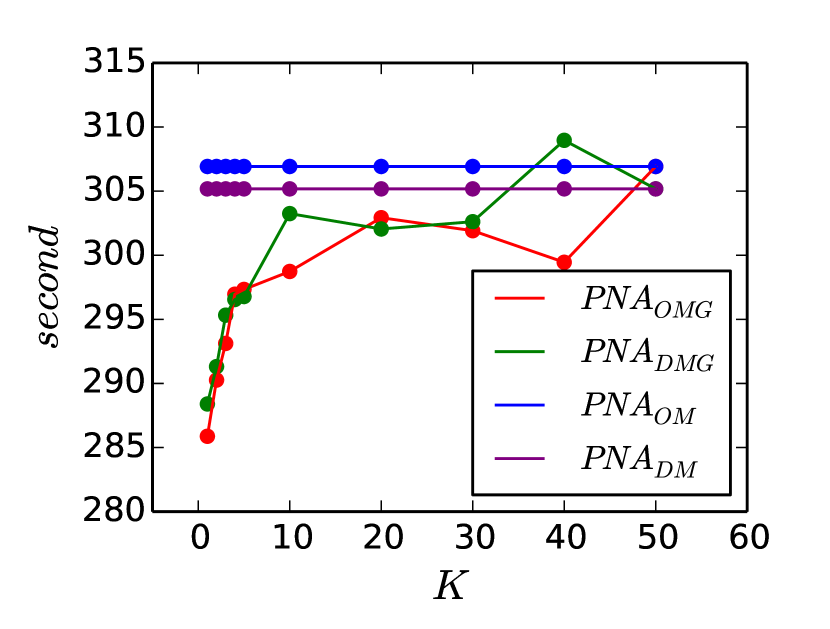
Figure 7: Time cost of PNAomg and PNAdmg with different partial matching rates.

VI Related Works

Aligned social network studies have become a hot research topic in recent years. Kong et al. [14] are the first to propose the anchor link prediction problem in fully aligned social networks. Zhang et al. [36, 37, 42, 40] propose to predict links for new users and new networks by transferring heterogeneous information across aligned social networks. A comprehensive survey about link prediction problems across multiple social networks is available in [38]. In addition to link prediction problems, Jin and Zhang et al. [12, 39, 41] introduce the community detection problems across aligned networks and Zhan et al. [35] study the information diffusion across aligned social networks.

Meta path first proposed by Sun et al. [26] has become a powerful tool, which can be applied in either in link prediction problems [26, 27] or clustering problems [28, 25]. Sun et al. [26] propose to predict co-author relationship in heterogeneous bibliographic networks based on meta path. Sun et al. extend the link prediction model to relationship prediction model based on meta path in [27]. Sun et al. [28] propose to calculate the similarity scores among users based on meta path in bibliographical network. Sun et al. [25] also apply meta path in clustering problem of heterogeneous information networks with incomplete attributes.

Tensor has been widely used in social networks studies. Moghaddam et al. [21] propose to apply extended tensor factorization model for personalized prediction of review helpfulness. Liu et al. [17] present a tensor-based framework for integrating heterogeneous multi-view data in the context of spectral clustering. A more detailed tutorial about tensor decomposition and applications is available in [13].

Class imbalance problems in classification can be very common in real-world applications. Chawla et al. [4] propose a technique for over-sampling the minority class with generated new synthetic minority instances. Kubat et al. [15] propose to address the class imbalance problems with under sampling of the majority cases in the training set. A systematic study of the class imbalance problem is available in [11].

College admission problem [23] and stable marriage problem [10] have been studied for many years and lots of works have been done in the last century. In recent years, some new papers have come out in these areas. Sotomayor et al. [24] propose to analyze the stability of the equilibrium outcomes in the admission games induced by stable matching rules. Ma [18] analyzes the truncation in stable matching and the small core in nash equilibrium in college admission problems. Floréen et al. [8] propose to study the almost stable matching by truncating the Gale-Shapley algorithm.

VII Conclusion

In this paper, we study the partial network alignment problem across partially aligned social networks. To address the challenges of the studied problem, a new method PNA is proposed in this paper. PNA can extract features for anchor links based on a set of anchor meta paths and overcome the class imbalance problem with over sampling and down sampling. PNA can effectively prune the non-existing anchor links with generic stable matching to ensure the results can meet the $one-to-one_{\leq}$ constraint. Extensive experiments done on two real-world partially aligned networks show the superior performance of PNA in addressing the partial network alignment problem.

VIII Acknowledgement

This work is supported in part by NSF through grants CNS-1115234, Google Research Award, the Pinnacle Lab at Singapore Management University, and Huawei grants.

References

- [1] M. Bayati, M. Gerritsen, D. Gleich, A. Saberi, and Y. Wang. Algorithms for large, sparse network alignment problems. In ICDM, 2009.
- [2] I. Bhattacharya and L. Getoor. Collective entity resolution in relational data. TKDD, 1(1), 2007.
- [3] N. Chawla. Data mining for imbalanced datasets: An overview. In Data Mining and Knowledge Discovery Handbook. 2005.
- [4] N. Chawla, K. Bowyer, L. Hall, and P. Kegelmeyer. Smote: Synthetic minority over-sampling technique. J. Artif. Int. Res., 2002.
- [5] L. Dubins and D. Freedman. Machiavelli and the gale-shapley algorithm. The American Mathematical Monthly, 1981.
- [6] M. Duggan and A. Smith. Social media update 2013. 2013. Report available at http://www.pewinternet.org/2013/12/30/social-media-update-2013/.
- [7] J. Euzenat and P. Shvaiko. Ontology Matching. Springer-Verlag New York, Inc., Secaucus, NJ, USA, 2007.
- [8] P. Floréen, P. Kaski, V. Polishchuk, and J. Suomela. Almost stable matchings by truncating the gale-shapley algorithm. Algorithmica, 2010.
- [9] D. Gale and L. Shapley. College admissions and the stability of marriage. The American Mathematical Monthly, 1962.
- [10] D. Gusfield and R. Irving. The Stable Marriage Problem: Structure and Algorithms. 1989.
- [11] N. Japkowicz and S. Stephen. The class imbalance problem: A systematic study. Intelligent Data Analysis, 2002.
- [12] S. Jin, J. Zhang, P. Yu, S. Yang, and A. Li. Synergistic partitioning in multiple large scale social networks. In IEEE BigData, 2014.
- [13] T. Kolda and B. Bader. Tensor decompositions and applications. SIAM REVIEW, 2009.
- [14] X. Kong, J. Zhang, and P. Yu. Inferring anchor links across heterogeneous social networks. In CIKM, 2013.
- [15] M. Kubat and S. Matwin. Addressing the curse of imbalanced training sets: One-sided selection. In ICML, 1997.
- [16] R. Lichtenwalter, J. Lussier, and N. Chawla. New perspectives and methods in link prediction. In KDD, 2010.
- [17] X. Liu, S. Ji, W. Glanzel, and B. De Moor. Multiview partitioning via tensor methods. TKDE, 2013.
- [18] J. Ma. Stable matchings and the small core in nash equilibrium in the college admissions problem. Technical report, 1998.
- [19] MarketingCharts. Majority of twitter users also use instagram. 2014. Report available at http://www.marketingcharts.com/wp/online/majority-of-twitter-users-also-use-instagram-38941/.
- [20] A. Menon and C. Elkan. Link prediction via matrix factorization. In ECML/PKDD, 2011.
- [21] S. Moghaddam, M. Jamali, and M. Ester. Etf: Extended tensor factorization model for personalizing prediction of review helpfulness. In WSDM, 2012.
- [22] O. Peled, M. Fire, L. Rokach, and Y. Elovici. Entity matching in online social networks. In SOCIALCOM, 2013.
- [23] A. Roth. The college admissions problem is not equivalent to the marriage problem. Journal of Economic Theory, 1985.
- [24] M. Sotomayor. The stability of the equilibrium outcomes in the admission games induced by stable matching rules. International Journal of Game Theory, 2008.
- [25] Y. Sun, C. Aggarwal, and J. Han. Relation strength-aware clustering of heterogeneous information networks with incomplete attributes. VLDB, 2012.
- [26] Y. Sun, R. Barber, M. Gupta, C. Aggarwal, and J. Han. Co-author relationship prediction in heterogeneous bibliographic networks. In ASONAM, 2011.
- [27] Y. Sun, J. Han, C. Aggarwal, and N. Chawla. When will it happen?: Relationship prediction in heterogeneous information networks. In WSDM, 2012.
- [28] Y. Sun, J. Han, X. Yan, P. Yu, and T. Wu. Pathsim: Meta path-based top-k similarity search in heterogeneous information networks. In VLDB, 2011.
- [29] J. Tang, H. Gao, X. Hu, and H. Liu. Exploiting homophily effect for trust prediction. In WSDM, 2013.
- [30] I. Tomek. Two Modifications of CNN. IEEE Transactions on Systems, Man and Cybernetics, 1976.
- [31] K. Wilcox and A. T. Stephen. Are close friends the enemy? online social networks, self-esteem, and self-control. Journal of Consumer Research, 2012.
- [32] Y. Yao, H. Tong, X. Yan, F. Xu, and J. Lu. Matri: a multi-aspect and transitive trust inference model. In WWW, 2013.
- [33] J. Ye, H. Cheng, Z. Zhu, and M. Chen. Predicting positive and negative links in signed social networks by transfer learning. In WWW, 2013.
- [34] R. Zafarani and H. Liu. Connecting users across social media sites: A behavioral-modeling approach. In KDD, 2013.
- [35] Q. Zhan, S. Wang J. Zhang, P. Yu, and J. Xie. Influence maximization across partially aligned heterogenous social networks. In PAKDD, 2015.
- [36] J. Zhang, X. Kong, and P. Yu. Predicting social links for new users across aligned heterogeneous social networks. In ICDM, 2013.
- [37] J. Zhang, X. Kong, and P. Yu. Transferring heterogeneous links across location-based social networks. In WSDM, 2014.
- [38] J. Zhang and P. Yu. Link prediction across heterogeneous social networks: A survey. Technical report, 2014.
- [39] J. Zhang and P. Yu. Community detection for emerging networks. In SDM, 2015.
- [40] J. Zhang and P. Yu. Integrated anchor and social link predictions across partially aligned social networks. In IJCAI, 2015.
- [41] J. Zhang and P. Yu. Mcd: Mutual clustering across multiple heterogeneous networks. In IEEE BigData Congress, 2015.
- [42] J. Zhang, P. Yu, and Z. Zhou. Meta-path based multi-network collective link prediction. In KDD, 2014.