XLES Part I: Introduction to Extended Large Eddy Simulation

Christoph Glawe Christoph.Glawe@protonmail.com Heiko Schmidt Alan R. Kerstein Rupert Klein BTU Cottbus-Senftenberg, Siemens-Halske-Ring 14, 03046 Cottbus, Germany 72 Lomitas Road, Danville, CA 94526, USA FU Berlin, Arnimallee 6, 14195 Berlin, Germany
Abstract

Direct numerical simulation (DNS), mostly used in fundamental turbulence research, is limited to low turbulent intensities due the current and future computer resources. Standard turbulence models, like RaNS (Reynolds averaged Navier-Stokes) and LES (Large Eddy Simulation), are applied to flows in engineering, but they miss small scale effects, which are frequently of importance, see e.g. the whole area of reactive flows, flows with apparent Prandtl or Schmidt number effects, or even wall bounded flows. A recent alternative to these standard approaches is the one-dimensional turbulence (ODT) model, which is limited to 1D sub-domains. In two papers we will provide a generalized filter strategy, called XLES (extended LES), including a formal theory (part I) and one special approach in the XLES family of models, called ODTLES (in part II (see Glawe et al. (2015))). ODTLES uses an ODT sub-grid model to describe all turbulent scales not represented by XLES, which leaves the larger scales to be simulated in 3D. This allows a turbulence modeling approach with a 3D resolution mainly independent of the turbulent intensity. Thus ODTLES is able to compute highly turbulent flows in domains of moderate complexity affordably and including the full range of turbulent and diffusive scales. The convergence of XLES to DNS is shown and the unconventional XLES advection approach is investigated in basic numerical tests. In part II, highly turbulent channel and duct flow results are discussed and show the future potential of XLES and ODTLES.

keywords:
Turbulence Modeling , Large Eddy Simulation , Channel Flow
journal: Journal of Computational Physics

1 Introduction

Turbulence is a ubiquitous effect in the physical world, with major technological and environmental impacts on human society and even human existence. Turbulence influenced the density and associated gravity variations that led to the formation of present-day galaxies, stars, and planets. Without turbulent mixing, planetary atmospheric phenomena such as clouds, storms, and precipitation essential for life on Earth would be unimaginably different. Turbulence in the ocean has innumerable effects on oceanic biota, starting with the commingling of phytoplankton with needed nutrients. Due to its broad influence and baffling complexity, progress in fundamental and practical understanding of turbulent mixing is exceptionally challenging, yet crucial for scientific advancement encompassing a wide class of problems in earth science, astrophysics, and engineering. For such problems, better understanding of turbulence interactions with buoyancy effects and chemical and thermodynamic processes is equally important. Due to its huge complexity, progress in understanding and prediction of turbulence is extremely challenging, yet crucial for scientific advancement in many disciplines.

Analytic solutions of turbulent flows cannot be derived for real life applications, e.g. with complex boundary conditions. Many meteorological and technical turbulent flows are investigated by numerical simulations. However the theoretical analysis of the governing equations is important to derive and improve simplifying models.

There are several possible levels of turbulence modeling commonly applied. The simplest model is no model: Direct Numerical Simulation (DNS) resolves all turbulent scales. Thus impacts of modeling and numerical errors are not influencing the investigated physics. DNS is widely used in fundamental research, but limited to moderate Reynolds numbers Re𝑅𝑒Re (until now Reτ5200𝑅subscript𝑒𝜏5200Re_{\tau}\approx 5200 for wall-bounded flows by Lee and Moser (2014)) and Rayleigh numbers Ra𝑅𝑎Ra due to the high computational effort, while many real-world flows have Reτ106greater-than-or-equivalent-to𝑅subscript𝑒𝜏superscript106Re_{\tau}\gtrsim 10^{6} (following Smits and Marusic (2013)).

In many industrial and some research applications Reynolds-Averaged Navier-Stokes equations (RaNS equations) are solved, because highly turbulent flows (e.g. Reτ>106𝑅subscript𝑒𝜏superscript106Re_{\tau}>10^{6}) corresponding to realistic flows are computationally feasible. RaNS describes the dynamics of time-averaged fields. The influence of fluctuating terms is modeled. Various models are known (see e.g. Spalart and Allmaras (1992) or an overview by Pope (2000)). RaNS is used for steady states, but is generally not useful for computing time-accurate flow statistics.

In recent years, Large Eddy Simulation (LES) has increasingly been used for industrial applied and fundamental turbulent flows. In LES spatially filtered equations are numerically solved while the unresolved sub-grid scale (SGS) terms are modeled e.g. by an eddy viscosity model (see e.g. Germano et al. (1991)).

Even in very fundamental highly turbulent flows LES need to resolve a wide range of scales including at least some portion of the inertial range of the turbulent cascade, which limits the achievable Reynolds numbers relative to the achievable Reynolds numbers in RaNS simulations. The parameterization of a certain range of small scales in RaNS and LES is especially problematic for multi-physics regimes such as buoyant and reacting flows because much of the complexity is thus relegated to the unresolved small scales.

For further details on LES we refer to standard literature (e.g. by Sagaut (2006)). For an overview of turbulence properties and other model approaches we refer to the work by Pope (2000).

Alternative model approaches e.g. the one-dimensional turbulence (ODT) model (see e.g. Kerstein (1999) and Kerstein et al. (2001)) describe the 3D turbulence within a 1D sub-domain including the full turbulent cascade, whereby the numerical representation of molecular diffusive effects becomes computationally feasible also in highly turbulent flows. Recently Meiselbach (2015) described wall bounded flows with Reτ6×10⁵𝑅subscript𝑒𝜏6superscript105Re_{\tau}\leq 6\times 10^{5} using an adaptive ODT version (by Lignell et al. (2013)), which is clearly in the range of real-world applications, but limited to applications that are reasonable within a 1D sub-domain.

To benefit from the ability of 1D models to describe highly turbulent flows, several approaches combine 1D models with LES, e.g. LES-ODT (e.g. by Cao and Echekki (2008)), LES/LEMLESLEM\rm LES/LEM (by Menon and Kerstein (2011)), and LEM3D (e.g. by Sannan et al. (2013)). Since ODT fully resolves e.g. molecular diffusion effects, it is fairly non-trivial to include it into an LES-like filter approach.

In this work we introduce an extended LES (XLES) filter approach, which is tailored to include 1D models as sub-grid models and can describe highly turbulent flows in a domain of moderate complexity, relevant e.g. in atmospheric science. To achieve this, XLES solves 2D filtered equations on a structured grid, maintaining one highly resolved Cartesian direction (this e.g. allows resolved molecular diffusion within an ODT sub-grid model). To derive a preferably general model, all Cartesian directions are treated equally: Three 2D filters, each corresponding to one highly resolved Cartesian direction, are applied independently to the governing equation. This leads to three coupled sets of 2D filtered equations, derived in section 2.

Thereby XLES only needs to resolve global 3D structures (e.g. the computational domain) independent of the turbulent cascade, while e.g. a one-dimensional turbulence model oriented in the respective highly resolved directions efficiently exploits the special symmetry of a 2D filter and represents the XLES microscale terms, corresponding to turbulent velocity scales not resolved by XLES. This ODTLES approach, investigated in detail in part II (Glawe et al. (2015)), is beneficial for flows with turbulent small scale effects playing an important role, e.g. in the combustion area, in buoyant stratified flows and wall-bounded flows with high turbulent intensity e.g. with high Reynolds or Rayleigh numbers.

This XLES based ODTLES model is an extended version of the ODTLES model, introduced and examined by Schmidt et al. (2008), Gonzalez-Juez et al. (2011), and Glawe et al. (2013).

In this work we distinguish between the expressions XLES to describe the XLES approach including an approximation or model for arising microscale terms, ODTLES if these terms are in particular described by ODT and XLES-U (XLES unclosed), if microscale terms are neglected.

In this work the XLES approach is introduced (in section 2) and XLES-U is verified by numerical studies and applied to a turbulent channel flow (in section 3), followed by conclusions in section 4. In Part II (see Glawe et al. (2015)) ODTLES is derived as one special approach in the XLES family of models and highly turbulent ODTLES channel and duct flow results are presented.

Note that in this work no Einstein summation convention is used.

2 Extended Large Eddy Simulation (XLES)

We consider the turbulent flow to be described by the incompressible Navier-Stokes equations for a Newtonian fluid including the conservation of mass in Eq. (1) and momentum in Eq. (2):

00\displaystyle 0 =j=13xjujabsentsuperscriptsubscript𝑗13subscriptsubscript𝑥𝑗subscript𝑢𝑗\displaystyle=\sum_{j=1}^{3}\partial_{x_{j}}u_{j} (1)
00\displaystyle 0 =1ρ0xip+[tνj=13xj2]ui+j=13xjujuiabsent1subscript𝜌0subscriptsubscript𝑥𝑖𝑝delimited-[]subscript𝑡𝜈superscriptsubscript𝑗13superscriptsubscriptsubscript𝑥𝑗2subscript𝑢𝑖superscriptsubscript𝑗13subscriptsubscript𝑥𝑗subscript𝑢𝑗subscript𝑢𝑖\displaystyle=\frac{1}{\rho_{0}}\partial_{x_{i}}p+\left[\partial_{t}-\nu\sum_{j=1}^{3}\partial_{x_{j}}^{2}\right]u_{i}+\sum_{j=1}^{3}\partial_{x_{j}}u_{j}\cdot u_{i} (2)

with the velocity uisubscript𝑢𝑖u_{i} in Cartesian xisubscript𝑥𝑖x_{i}-direction (i={1,2,3}𝑖123i=\{1,2,3\}), a constant kinematic viscosity ν𝜈\nu, and the pressure gradient xipsubscriptsubscript𝑥𝑖𝑝\partial_{x_{i}}p. For simplicity we assume in this work the constant density to be ρ0=1subscript𝜌01\rho_{0}=1.

Variables e.g. the velocities uisubscript𝑢𝑖u_{i} and operators are assumed to be described within a continuum. Discrete variables are marked with the superscript d𝑑{d} (e.g. discrete velocities: uidsuperscriptsubscript𝑢𝑖𝑑u_{i}^{{d}}).

Similar to LES, in XLES the velocity field is filtered. 3D filter functions commonly applied in LES are defined as tensor products of 1D filter functions [lk]delimited-[]subscript𝑙𝑘[l_{k}] (we are using an operator notation) in xksubscript𝑥𝑘x_{k}-direction (k={1,2,3}𝑘123k=\{1,2,3\}; a filter operating on a continuum corresponds to a convolution). To derive macroscale (to be simulated) and microscale (to be modeled) terms the spatial scales are separated for modeling purpose using these 1D filter operators:

ui=subscript𝑢𝑖absent\displaystyle u_{i}= [𝟙𝟙𝟙]uidelimited-[]double-struck-𝟙double-struck-𝟙double-struck-𝟙subscript𝑢𝑖\displaystyle\left[\mathbb{1}\,\mathbb{1}\,\mathbb{1}\right]u_{i} (3)
=\displaystyle= [(l1+(𝟙l1))(l2+(𝟙l2))(l3+(𝟙l3))]uidelimited-[]subscript𝑙1double-struck-𝟙subscript𝑙1subscript𝑙2double-struck-𝟙subscript𝑙2subscript𝑙3double-struck-𝟙subscript𝑙3subscript𝑢𝑖\displaystyle\left[(l_{1}+(\mathbb{1}-l_{1}))(l_{2}+(\mathbb{1}-l_{2}))(l_{3}+(\mathbb{1}-l_{3}))\right]u_{i}
\displaystyle\equiv [(l1+s1)(l2+s2)(l3+s3)]uidelimited-[]subscript𝑙1subscript𝑠1subscript𝑙2subscript𝑠2subscript𝑙3subscript𝑠3subscript𝑢𝑖\displaystyle\left[(l_{1}+s_{1})(l_{2}+s_{2})(l_{3}+s_{3})\right]u_{i}
=\displaystyle= [l1l2l3+s1l2l3+l1s2l3+l1l2s3+s1s2l3+s1l2s3+l1s2s3+s1s2s3]uidelimited-[]subscript𝑙1subscript𝑙2subscript𝑙3subscript𝑠1subscript𝑙2subscript𝑙3subscript𝑙1subscript𝑠2subscript𝑙3subscript𝑙1subscript𝑙2subscript𝑠3subscript𝑠1subscript𝑠2subscript𝑙3subscript𝑠1subscript𝑙2subscript𝑠3subscript𝑙1subscript𝑠2subscript𝑠3subscript𝑠1subscript𝑠2subscript𝑠3subscript𝑢𝑖\displaystyle\left[{l_{1}l_{2}l_{3}+s_{1}l_{2}l_{3}+l_{1}s_{2}l_{3}+l_{1}l_{2}s_{3}}+s_{1}s_{2}l_{3}+s_{1}l_{2}s_{3}+l_{1}s_{2}s_{3}+s_{1}s_{2}s_{3}\right]u_{i}

with the unity operator [𝟙]delimited-[]double-struck-𝟙[\mathbb{1}] and the 1D small scale operator

[sk]=[𝟙lk].delimited-[]subscript𝑠𝑘delimited-[]double-struck-𝟙subscript𝑙𝑘\displaystyle[s_{k}]=[\mathbb{1}-l_{k}]. (4)

The tensor product ansatz causes combinations of 1D operators to be commutable, e.g. s1l2l3=l3s1l2subscript𝑠1subscript𝑙2subscript𝑙3subscript𝑙3subscript𝑠1subscript𝑙2s_{1}l_{2}l_{3}=l_{3}s_{1}l_{2}.

In general the occurring spatial 3D scales (terms in the last row of Eq. (3)) are decomposed into those to be simulated (resolved) and those to be modeled (unresolved). We will refer to this as ‘filter separation’, because the commonly used term ‘scale separation’ implies the simulated scales to be large. In LES the resolved velocities correspond to the 3D large scale field [l1l2l3]uidelimited-[]subscript𝑙1subscript𝑙2subscript𝑙3subscript𝑢𝑖[l_{1}l_{2}l_{3}]u_{i}. Thus the LES filter separation corresponds to a 3D scale separation.

In table 1 the filter separations are compared between LES, DNS and XLES.

Table 1: Comparison of filter separation ansatzes
Model resolved scales unresolved scales (SGS)
LES u¯iLES=[l1l2l3]uisuperscriptsubscript¯𝑢𝑖LESdelimited-[]subscript𝑙1subscript𝑙2subscript𝑙3subscript𝑢𝑖\overline{u}_{i}^{\rm LES}=[l_{1}l_{2}l_{3}]u_{i} u~iLES=[s1l2l3+l1s2l3+l1l2s3\widetilde{u}_{i}^{\rm LES}=[s_{1}l_{2}l_{3}+l_{1}s_{2}l_{3}+l_{1}l_{2}s_{3}
+s1s2l3+s1l2s3+l1s2s3+s1s2s3]ui+s_{1}s_{2}l_{3}+s_{1}l_{2}s_{3}+l_{1}s_{2}s_{3}+s_{1}s_{2}s_{3}]u_{i}
DNS [𝟙𝟙𝟙]uidelimited-[]double-struck-𝟙double-struck-𝟙double-struck-𝟙subscript𝑢𝑖[\mathbb{1}\,\mathbb{1}\,\mathbb{1}]u_{i} 00
XLES u¯i=subscript¯𝑢𝑖absent\overline{u}_{i}= u~i=subscript~𝑢𝑖absent\widetilde{u}_{i}=
[l1l2l3+s1l2l3+l1s2l3+l1l2s3]uidelimited-[]subscript𝑙1subscript𝑙2subscript𝑙3subscript𝑠1subscript𝑙2subscript𝑙3subscript𝑙1subscript𝑠2subscript𝑙3subscript𝑙1subscript𝑙2subscript𝑠3subscript𝑢𝑖[l_{1}l_{2}l_{3}+s_{1}l_{2}l_{3}+l_{1}s_{2}l_{3}+l_{1}l_{2}s_{3}]u_{i} [s1s2l3+s1l2s3+l1s2s3+s1s2s3]uidelimited-[]subscript𝑠1subscript𝑠2subscript𝑙3subscript𝑠1subscript𝑙2subscript𝑠3subscript𝑙1subscript𝑠2subscript𝑠3subscript𝑠1subscript𝑠2subscript𝑠3subscript𝑢𝑖[s_{1}s_{2}l_{3}+s_{1}l_{2}s_{3}+l_{1}s_{2}s_{3}+s_{1}s_{2}s_{3}]u_{i}

The LES resolved (large scale) velocities are u¯iLES=[l1l2l3]uisuperscriptsubscript¯𝑢𝑖LESdelimited-[]subscript𝑙1subscript𝑙2subscript𝑙3subscript𝑢𝑖\bar{u}_{i}^{\rm LES}=[l_{1}l_{2}l_{3}]u_{i}, and the unresolved (SGS) velocities u~iLES=[𝟙l1l2l3]uisuperscriptsubscript~𝑢𝑖LESdelimited-[]double-struck-𝟙subscript𝑙1subscript𝑙2subscript𝑙3subscript𝑢𝑖\tilde{u}_{i}^{\rm LES}=[\mathbb{1}-l_{1}l_{2}l_{3}]u_{i}. The acronym LESLES{\rm LES} is used to differentiate between standard LES velocities and those defined in XLES.

In DNS all available scales are resolved numerically.

In XLES the resolved scales are connected to 2D filtered fields. Without loss of generality (w.l.o.g.) we apply [l1l2]delimited-[]subscript𝑙1subscript𝑙2[l_{1}l_{2}] leading to:

[l1l2]ui=[l1l2l3+l1l2s3]ui.delimited-[]subscript𝑙1subscript𝑙2subscript𝑢𝑖delimited-[]subscript𝑙1subscript𝑙2subscript𝑙3subscript𝑙1subscript𝑙2subscript𝑠3subscript𝑢𝑖\displaystyle[l_{1}l_{2}]u_{i}=[l_{1}l_{2}l_{3}+l_{1}l_{2}s_{3}]u_{i}. (5)

To treat all Cartesian directions equally, all possible 2D-filtered terms [l2l3]uidelimited-[]subscript𝑙2subscript𝑙3subscript𝑢𝑖[l_{2}l_{3}]u_{i}, [l1l3]uidelimited-[]subscript𝑙1subscript𝑙3subscript𝑢𝑖[l_{1}l_{3}]u_{i}, and [l1l2]uidelimited-[]subscript𝑙1subscript𝑙2subscript𝑢𝑖[l_{1}l_{2}]u_{i} are resolved numerically.

This XLES macroscale (to be simulated) approach can be interpreted as the LES macroscale ([l1l2l3]delimited-[]subscript𝑙1subscript𝑙2subscript𝑙3[l_{1}l_{2}l_{3}]) with additionally 1D resolved small scale (RSS) terms in all Cartesian directions ([s1l2l3]+[l1s2l3]+[l1l2s3]delimited-[]subscript𝑠1subscript𝑙2subscript𝑙3delimited-[]subscript𝑙1subscript𝑠2subscript𝑙3delimited-[]subscript𝑙1subscript𝑙2subscript𝑠3[s_{1}l_{2}l_{3}]+[l_{1}s_{2}l_{3}]+[l_{1}l_{2}s_{3}]). Both, the XLES resolved velocity scales (investigated in this work) and the unresolved scales (investigated in part II (Glawe et al. (2015))) impose special requirements on the numerical scheme and modeling; techniques known from LES cannot be applied one-to-one to XLES.

2.1 XLES: Spatial Filtering

In XLES, 2D filter operators -each corresponding to one highly resolved Cartesian direction- are applied to the governing equations, comparable to the 3D filtering in LES. To derive a filter approach, independent of the chosen Cartesian direction, three 2D filters, corresponding to three Cartesian directions, are applied. We will use a vector notation (called XLES vector notation), indicated by an underbar (e.g. u¯isubscript¯𝑢𝑖\underline{u}_{i}). Each vector element contains one of the three 2D filtered velocity fields:

([l2l3]ui[l1l3]ui[l1l2]ui)=(l2l3000l1l3000l1l2)(uiuiui)l¯¯2Du¯iu¯^imatrixdelimited-[]subscript𝑙2subscript𝑙3subscript𝑢𝑖delimited-[]subscript𝑙1subscript𝑙3subscript𝑢𝑖delimited-[]subscript𝑙1subscript𝑙2subscript𝑢𝑖matrixsubscript𝑙2subscript𝑙3000subscript𝑙1subscript𝑙3000subscript𝑙1subscript𝑙2matrixsubscript𝑢𝑖subscript𝑢𝑖subscript𝑢𝑖superscript¯¯𝑙2𝐷subscript¯𝑢𝑖subscript^¯𝑢𝑖\displaystyle\begin{pmatrix}[l_{2}l_{3}]{u}_{i}\\ [l_{1}l_{3}]{u}_{i}\\ [l_{1}l_{2}]{u}_{i}\end{pmatrix}=\begin{pmatrix}l_{2}l_{3}&0&0\\ 0&l_{1}l_{3}&0\\ 0&0&l_{1}l_{2}\end{pmatrix}\begin{pmatrix}{u}_{i}\\ {u}_{i}\\ {u}_{i}\end{pmatrix}\equiv\underline{\underline{l}}^{2D}\,\underline{u}_{i}\equiv\hat{\underline{u}}_{i} (6)

with the 2D filter matrix l¯¯2Dsuperscript¯¯𝑙2𝐷\underline{\underline{l}}^{2D}.

The 2D filtered velocity fields u¯^isubscript^¯𝑢𝑖\hat{\underline{u}}_{i} (we refer to u¯^isubscript^¯𝑢𝑖\hat{\underline{u}}_{i} as the XLES vector) are discretized using three overlapping staggered XLES-grids with face-centered velocities and cell-centered pressure, illustrated in figure 1(b)1(d), where each XLES-grid k={1,2,3}𝑘123k=\{1,2,3\} discretizes one XLES vector element u^k,idsuperscriptsubscript^𝑢𝑘𝑖𝑑\hat{{u}}_{k,i}^{d}. The size of the discrete 1D filter [lkd]delimited-[]superscriptsubscript𝑙𝑘𝑑[l_{k}^{d}] corresponds to the large scale cell size ΔxkLESΔsuperscriptsubscript𝑥𝑘LES\Delta x_{k}^{\rm LES} (see figure 1(a)), where the discrete 1D filter definition [lkd]delimited-[]superscriptsubscript𝑙𝑘𝑑[l_{k}^{d}] corresponds to a box filter

[lkd]ui=1ΔxkLESΔxkLES2ΔxkLES2uidxk.delimited-[]superscriptsubscript𝑙𝑘𝑑subscript𝑢𝑖1Δsuperscriptsubscript𝑥𝑘LESsuperscriptsubscriptΔsuperscriptsubscript𝑥𝑘LES2Δsuperscriptsubscript𝑥𝑘LES2subscript𝑢𝑖differential-dsuperscriptsubscript𝑥𝑘\displaystyle[l_{k}^{d}]u_{i}=\frac{1}{\Delta x_{k}^{\rm LES}}\int_{-\frac{\Delta x_{k}^{\rm LES}}{2}}^{\frac{\Delta x_{k}^{\rm LES}}{2}}u_{i}{\rm\,d}x_{k}^{\prime}. (7)

Here the discrete mesh corresponds to the discrete filter size which is often called implicit filtering.

Refer to caption
(a) LES grid:
u¯id,LES[l1l2l3]uisuperscriptsubscript¯𝑢𝑖𝑑LESdelimited-[]subscript𝑙1subscript𝑙2subscript𝑙3subscript𝑢𝑖\overline{u}_{i}^{d,\textrm{LES}}\approx[l_{1}l_{2}l_{3}]u_{i}.
Refer to caption
(b) Grid 1:
u^1,id[l2l3]uisuperscriptsubscript^𝑢1𝑖𝑑delimited-[]subscript𝑙2subscript𝑙3subscript𝑢𝑖\hat{u}_{1,i}^{d}\approx[l_{2}l_{3}]u_{i}.
Refer to caption
(c) Grid 2:
u^2,id[l1l3]uisuperscriptsubscript^𝑢2𝑖𝑑delimited-[]subscript𝑙1subscript𝑙3subscript𝑢𝑖\hat{u}_{2,i}^{d}\approx[l_{1}l_{3}]u_{i}.
Refer to caption
(d) Grid 3:
u^3,id[l1l2]uisuperscriptsubscript^𝑢3𝑖𝑑delimited-[]subscript𝑙1subscript𝑙2subscript𝑢𝑖\hat{u}_{3,i}^{d}\approx[l_{1}l_{2}]u_{i}.
Figure 1: In XLES the velocities are resolved using multiple XLES-grids illustrated in 1(b)-1(d). 3D large scale properties, corresponding to a standard LES grid are for illustration represented with NLES=4subscript𝑁LES4N_{\rm LES}=4 cells per direction in 1(a). In XLES the 3D large scale velocities are derived by 1D filtering the XLES properties: u¯iLES=[lk]u^k,i,k={1,2,3}formulae-sequencesuperscriptsubscript¯𝑢𝑖LESdelimited-[]subscript𝑙𝑘subscript^𝑢𝑘𝑖𝑘123\overline{u}_{i}^{\rm LES}=[l_{k}]\hat{u}_{k,i},\;k=\{1,2,3\}. The discrete XLES resolved small scale (‘RSS’) properties are represented for illustration by NRSS=16subscript𝑁RSS16N_{\rm RSS}=16 cells in 1(b)-1(d).

The XLES filter separation decomposes the full velocity field into three parts (using the XLES vector notation):

u¯isubscript¯𝑢𝑖\displaystyle\underline{u}_{i} (uiuiui)=([l2l3]ui[l1l3]ui[l1l2]ui)+([l1s2l3+l1l2s3]ui[s1l2l3+l1l2s3]ui[s1l2l3+l1s2l3]ui)+([𝒮]ui[𝒮]ui[𝒮]ui)absentmatrixsubscript𝑢𝑖subscript𝑢𝑖subscript𝑢𝑖matrixdelimited-[]subscript𝑙2subscript𝑙3subscript𝑢𝑖delimited-[]subscript𝑙1subscript𝑙3subscript𝑢𝑖delimited-[]subscript𝑙1subscript𝑙2subscript𝑢𝑖matrixdelimited-[]subscript𝑙1subscript𝑠2subscript𝑙3subscript𝑙1subscript𝑙2subscript𝑠3subscript𝑢𝑖delimited-[]subscript𝑠1subscript𝑙2subscript𝑙3subscript𝑙1subscript𝑙2subscript𝑠3subscript𝑢𝑖delimited-[]subscript𝑠1subscript𝑙2subscript𝑙3subscript𝑙1subscript𝑠2subscript𝑙3subscript𝑢𝑖matrixdelimited-[]𝒮subscript𝑢𝑖delimited-[]𝒮subscript𝑢𝑖delimited-[]𝒮subscript𝑢𝑖\displaystyle\equiv\begin{pmatrix}{u}_{i}\\ {u}_{i}\\ {u}_{i}\end{pmatrix}=\begin{pmatrix}[l_{2}l_{3}]{u}_{i}\\ [l_{1}l_{3}]{u}_{i}\\ [l_{1}l_{2}]{u}_{i}\end{pmatrix}+\begin{pmatrix}[l_{1}s_{2}l_{3}+l_{1}l_{2}s_{3}]u_{i}\\ [s_{1}l_{2}l_{3}+l_{1}l_{2}s_{3}]u_{i}\\ [s_{1}l_{2}l_{3}+l_{1}s_{2}l_{3}]u_{i}\end{pmatrix}+\begin{pmatrix}[\mathcal{S}]u_{i}\\ [\mathcal{S}]u_{i}\\ [\mathcal{S}]u_{i}\end{pmatrix}
l¯¯2Du¯i+C¯¯s¯¯1Dl¯¯2Du¯i+[𝒮]u¯i::absentsuperscript¯¯𝑙2𝐷subscript¯𝑢𝑖¯¯𝐶superscript¯¯𝑠1𝐷superscript¯¯𝑙2𝐷subscript¯𝑢𝑖delimited-[]𝒮subscript¯𝑢𝑖absent\displaystyle\equiv\underline{\underline{l}}^{2D}\,\underline{u}_{i}+\underline{\underline{C}}\,\underline{\underline{s}}^{1D}\underline{\underline{l}}^{2D}\underline{u}_{i}+[\mathcal{S}]\underline{u}_{i}: (8)
  1. 1.

    ‘Directly Resolved’:

    The 2D filter l¯¯2Dsuperscript¯¯𝑙2𝐷\underline{\underline{l}}^{2D} applied to the full velocity field leads to the XLES vector: u¯^i=l¯¯2Du¯isubscript^¯𝑢𝑖superscript¯¯𝑙2𝐷subscript¯𝑢𝑖\hat{\underline{u}}_{i}=\underline{\underline{l}}^{2D}\,\underline{u}_{i}. Each XLES-grid represents its own directly resolved velocity field distinct from the other XLES-grids.

  2. 2.

    ‘Indirectly Resolved’:

    There are indirectly resolved small scale terms (‘directly resolved’ by another XLES-grid): C¯¯s¯¯1Dl¯¯2Du¯i¯¯𝐶superscript¯¯𝑠1𝐷superscript¯¯𝑙2𝐷subscript¯𝑢𝑖\underline{\underline{C}}\,\underline{\underline{s}}^{1D}\underline{\underline{l}}^{2D}\underline{u}_{i}. Especially within non-linear advection terms (in Eq. (2)), they determine the coupling between the XLES-grids. The coupling matrix C¯¯¯¯𝐶\underline{\underline{C}} and the small scale matrix s¯¯1Dsuperscript¯¯𝑠1𝐷\underline{\underline{s}}^{1D} in Eq. (8) are:

    C¯¯=(0𝟙𝟙𝟙0𝟙𝟙𝟙0)ands¯¯1D=(s1000s2000s3).formulae-sequence¯¯𝐶matrix0double-struck-𝟙double-struck-𝟙double-struck-𝟙0double-struck-𝟙double-struck-𝟙double-struck-𝟙0andsuperscript¯¯𝑠1𝐷matrixsubscript𝑠1000subscript𝑠2000subscript𝑠3\displaystyle\underline{\underline{C}}=\begin{pmatrix}0&\mathbb{1}&\mathbb{1}\\ \mathbb{1}&0&\mathbb{1}\\ \mathbb{1}&\mathbb{1}&0\end{pmatrix}\,{\rm and}\quad\underline{\underline{s}}^{1D}=\begin{pmatrix}s_{1}&0&0\\ 0&s_{2}&0\\ 0&0&s_{3}\end{pmatrix}. (9)

    The matrix s¯¯1Dsuperscript¯¯𝑠1𝐷\underline{\underline{s}}^{1D} defines the resolved small scale (RSS) velocities u¯ˇisubscriptˇ¯𝑢𝑖\check{\underline{u}}_{i} (these are part of the XLES macroscale, contrary to LES):

    s¯¯1Du¯iu¯ˇi=u¯^il¯¯1Du¯^i=u¯^iu¯¯iLESsuperscript¯¯𝑠1𝐷subscript¯𝑢𝑖subscriptˇ¯𝑢𝑖subscript^¯𝑢𝑖superscript¯¯𝑙1𝐷subscript^¯𝑢𝑖subscript^¯𝑢𝑖superscriptsubscript¯¯𝑢𝑖LES\displaystyle\underline{\underline{s}}^{1D}\,\underline{u}_{i}\equiv\check{\underline{u}}_{i}=\hat{\underline{u}}_{i}-\underline{\underline{l}}^{1D}\hat{\underline{u}}_{i}=\hat{\underline{u}}_{i}-\overline{\underline{u}}_{i}^{\rm LES} (10)

    with the 1D filter matrix

    l¯¯1D=(l1000l2000l3).superscript¯¯𝑙1𝐷matrixsubscript𝑙1000subscript𝑙2000subscript𝑙3\displaystyle\underline{\underline{l}}^{1D}=\begin{pmatrix}l_{1}&0&0\\ 0&l_{2}&0\\ 0&0&l_{3}\end{pmatrix}. (11)

    In index notation: The term (w.l.o.g.) [l1s2l3]ui=[l1l3]ui[l1l2l3]uidelimited-[]subscript𝑙1subscript𝑠2subscript𝑙3subscript𝑢𝑖delimited-[]subscript𝑙1subscript𝑙3subscript𝑢𝑖delimited-[]subscript𝑙1subscript𝑙2subscript𝑙3subscript𝑢𝑖[l_{1}s_{2}l_{3}]u_{i}=[l_{1}l_{3}]u_{i}-[l_{1}l_{2}l_{3}]u_{i} can be interpreted numerically, because u^2,i=[l1l3]uisubscript^𝑢2𝑖delimited-[]subscript𝑙1subscript𝑙3subscript𝑢𝑖\hat{u}_{2,i}=[l_{1}l_{3}]u_{i} is exclusively available in XLES-grid 222 and the 1D filtered XLES velocity field [l2]u^2,i=[l1l2l3]uidelimited-[]subscript𝑙2subscript^𝑢2𝑖delimited-[]subscript𝑙1subscript𝑙2subscript𝑙3subscript𝑢𝑖[l_{2}]\hat{u}_{2,i}=[l_{1}l_{2}l_{3}]u_{i}, corresponding to the LES velocity field u¯iLESsuperscriptsubscript¯𝑢𝑖𝐿𝐸𝑆\overline{{u}}_{i}^{LES} (see figure 1), is also available in XLES-grid 222.

  3. 3.

    ‘Not Resolved’:

    The velocity scales [𝒮]ui=[s1s2l3+s1l2s3+l1s2s3+s1s2s3]uidelimited-[]𝒮subscript𝑢𝑖delimited-[]subscript𝑠1subscript𝑠2subscript𝑙3subscript𝑠1subscript𝑙2subscript𝑠3subscript𝑙1subscript𝑠2subscript𝑠3subscript𝑠1subscript𝑠2subscript𝑠3subscript𝑢𝑖[\mathcal{S}]u_{i}=[s_{1}s_{2}l_{3}+s_{1}l_{2}s_{3}+l_{1}s_{2}s_{3}+s_{1}s_{2}s_{3}]u_{i} are not resolved in any XLES-grid (XLES sub-grid scale (SGS) or XLES microscale). In part II (Glawe et al. (2015)) advection terms containing unresolved velocity scales are interpreted by the ODT model.

We summarize all resolved velocity scales (directly and indirectly):

u¯¯i=[l1l2l3+s1l2l3+l1s2l3+l1l2s3]u¯i=(l¯¯2D+C¯¯s¯¯1Dl¯¯2D)u¯i.subscript¯¯𝑢𝑖delimited-[]subscript𝑙1subscript𝑙2subscript𝑙3subscript𝑠1subscript𝑙2subscript𝑙3subscript𝑙1subscript𝑠2subscript𝑙3subscript𝑙1subscript𝑙2subscript𝑠3subscript¯𝑢𝑖superscript¯¯𝑙2𝐷¯¯𝐶superscript¯¯𝑠1𝐷superscript¯¯𝑙2𝐷subscript¯𝑢𝑖\displaystyle\overline{\underline{u}}_{i}=[l_{1}l_{2}l_{3}+s_{1}l_{2}l_{3}+l_{1}s_{2}l_{3}+l_{1}l_{2}s_{3}]\underline{u}_{i}=(\underline{\underline{l}}^{2D}+\underline{\underline{C}}\,\underline{\underline{s}}^{1D}\underline{\underline{l}}^{2D})\underline{u}_{i}. (12)

A possible interpretation of the XLES macroscale is the numerical approximation of u¯isubscript¯𝑢𝑖\overline{u}_{i} instead of u¯iLES=[l1l2l3]uisuperscriptsubscript¯𝑢𝑖LESdelimited-[]subscript𝑙1subscript𝑙2subscript𝑙3subscript𝑢𝑖\overline{u}_{i}^{\rm LES}=[l_{1}l_{2}l_{3}]u_{i} in LES (compare to table 1). A shows that expressing u¯¯isubscript¯¯𝑢𝑖\overline{\underline{u}}_{i} in index notation automatically leads to three coupled XLES-grids (corresponding to Eq. (12)).

2.2 Momentum Conservation

Similar to LES, in XLES filtered equations are solved. Contrary to LES the XLES equations are derived by applying a 2D filter matrix l¯¯2Dsuperscript¯¯𝑙2𝐷\underline{\underline{l}}^{2D} to the momentum equation Eq. (2) leading to (in XLES vector notation):

0=0absent\displaystyle 0= xip¯^+(tνj=13xj2)u¯^i+j=13xju¯^ju¯^i+j=13τ¯ijXLESsubscriptsubscript𝑥𝑖¯^𝑝subscript𝑡𝜈superscriptsubscript𝑗13superscriptsubscriptsubscript𝑥𝑗2subscript¯^𝑢𝑖superscriptsubscript𝑗13subscriptsubscript𝑥𝑗subscript¯^𝑢𝑗subscript¯^𝑢𝑖superscriptsubscript𝑗13superscriptsubscript¯𝜏𝑖𝑗XLES\displaystyle\partial_{x_{i}}\underline{\hat{p}}+\left(\partial_{t}-\nu\sum_{j=1}^{3}\partial_{x_{j}}^{2}\right)\underline{\hat{u}}_{i}+\sum_{j=1}^{3}\partial_{x_{j}}\underline{\hat{u}}_{j}*\underline{\hat{u}}_{i}+\sum_{j=1}^{3}\underline{\tau}_{ij}^{\rm XLES} (13)

with the 2D filtered pressure

p¯^=l¯¯2Dp¯=([l2l3]p[l1l3]p[l1l2]p)T,¯^𝑝superscript¯¯𝑙2𝐷¯𝑝superscriptmatrixdelimited-[]subscript𝑙2subscript𝑙3𝑝delimited-[]subscript𝑙1subscript𝑙3𝑝delimited-[]subscript𝑙1subscript𝑙2𝑝𝑇\displaystyle\underline{\hat{p}}=\underline{\underline{l}}^{2D}\underline{p}=\begin{pmatrix}[l_{2}l_{3}]p&[l_{1}l_{3}]p&[l_{1}l_{2}]p\end{pmatrix}^{T}, (14)

the XLES residual stress tensors τ¯ijXLESsuperscriptsubscript¯𝜏𝑖𝑗XLES\underline{\tau}_{ij}^{\rm XLES}, and the Hadamard operator *, an entry-wise multiplication between XLES vectors and matrices.

The three 2D filtered momentum equations, each describing three velocity components (hence the number of equations is tripled), coexist and are solved simultaneously.

Compared to LES advection terms xju¯jLESu¯jLESsubscriptsubscript𝑥𝑗superscriptsubscript¯𝑢𝑗LESsuperscriptsubscript¯𝑢𝑗LES\partial_{x_{j}}\overline{u}_{j}^{\rm LES}\overline{u}_{j}^{\rm LES} the XLES advection terms xju¯^ju¯^i=xj(u¯¯jLES+u¯ˇj)(u¯¯iLES+u¯ˇi)subscriptsubscript𝑥𝑗subscript¯^𝑢𝑗subscript¯^𝑢𝑖subscriptsubscript𝑥𝑗superscriptsubscript¯¯𝑢𝑗LESsubscriptˇ¯𝑢𝑗superscriptsubscript¯¯𝑢𝑖LESsubscriptˇ¯𝑢𝑖\partial_{x_{j}}\underline{\hat{u}}_{j}*\underline{\hat{u}}_{i}=\partial_{x_{j}}(\overline{\underline{u}}_{j}^{\rm LES}+\check{\underline{u}}_{j})*(\overline{\underline{u}}_{i}^{\rm LES}+\check{\underline{u}}_{i}) contain additional XLES-grid specific resolved small scale (RSS) terms.

The contribution associated with the XLES residual stress tensors

τ¯ijXLES=l¯¯2D(xju¯ju¯i)xju¯^ju¯^isuperscriptsubscript¯𝜏𝑖𝑗XLESsuperscript¯¯𝑙2𝐷subscriptsubscript𝑥𝑗subscript¯𝑢𝑗subscript¯𝑢𝑖subscriptsubscript𝑥𝑗subscript¯^𝑢𝑗subscript¯^𝑢𝑖\displaystyle\underline{\tau}_{ij}^{\rm XLES}=\underline{\underline{l}}^{2D}\left(\partial_{x_{j}}\underline{{u}{}}_{j}*\underline{{u}{}}_{i}\right)-\partial_{x_{j}}\underline{\hat{u}}_{j}*\underline{\hat{u}}_{i} (15)

is captured through the use of some form of modeling or approximation. To investigate the residual stresses in more detail, a 2D decomposition (a modified version of the 3D decomposition by Leonard (1975)) is performed, leading to:

τ¯ijXLESsuperscriptsubscript¯𝜏𝑖𝑗XLES\displaystyle\underline{\tau}_{ij}^{\rm XLES} =𝒳¯ijXLES+¯ij2D+𝒞¯ijXLES+¯ijXLESabsentsuperscriptsubscript¯𝒳𝑖𝑗XLESsubscriptsuperscript¯2𝐷𝑖𝑗superscriptsubscript¯𝒞𝑖𝑗XLESsuperscriptsubscript¯𝑖𝑗XLES\displaystyle=\mathcal{\underline{X}}_{ij}^{\rm XLES}+\mathcal{\underline{L}}^{2D}_{ij}+\mathcal{\underline{C}}_{ij}^{\rm XLES}+\mathcal{\underline{R}}_{ij}^{\rm XLES} (16)

where:

  • 1.

    XLES coupling tensor terms

    𝒳¯ijXLES=xj(u¯^jC¯¯s¯¯1Dl¯¯2Du¯i+C¯¯s¯¯1Dl¯¯2Du¯ju¯^i+C¯¯s¯¯1Dl¯¯2Du¯jC¯¯s¯¯1Dl¯¯2Du¯i)superscriptsubscript¯𝒳𝑖𝑗XLESsubscriptsubscript𝑥𝑗subscript^¯𝑢𝑗¯¯𝐶superscript¯¯𝑠1𝐷superscript¯¯𝑙2𝐷subscript¯𝑢𝑖¯¯𝐶superscript¯¯𝑠1𝐷superscript¯¯𝑙2𝐷subscript¯𝑢𝑗subscript^¯𝑢𝑖¯¯𝐶superscript¯¯𝑠1𝐷superscript¯¯𝑙2𝐷subscript¯𝑢𝑗¯¯𝐶superscript¯¯𝑠1𝐷superscript¯¯𝑙2𝐷subscript¯𝑢𝑖\displaystyle\mathcal{\underline{X}}_{ij}^{\rm XLES}=\partial_{x_{j}}\left(\hat{\underline{u}}_{j}*\underline{\underline{C}}\,\underline{\underline{s}}^{1D}\underline{\underline{l}}^{2D}{\underline{u}}_{i}+\underline{\underline{C}}\,\underline{\underline{s}}^{1D}\underline{\underline{l}}^{2D}{\underline{u}}_{j}*\hat{\underline{u}}_{i}+\underline{\underline{C}}\,\underline{\underline{s}}^{1D}\underline{\underline{l}}^{2D}{\underline{u}}_{j}*\underline{\underline{C}}\,\underline{\underline{s}}^{1D}\underline{\underline{l}}^{2D}{\underline{u}}_{i}\right) (17)

    involve ‘indirectly resolved’ terms. These stress terms couple the momentum equations represented by different XLES-grids. A possible approximation of 𝒳¯ijXLESsuperscriptsubscript¯𝒳𝑖𝑗XLES\mathcal{\underline{X}}_{ij}^{\rm XLES} is investigated in section 2.2.1. In LES these terms are not simulated and therefore typically modeled or approximated and contribute to 3D cross-stress and 3D SGS Reynolds stress terms.

  • 2.

    2D Leonard stresses

    ¯ij2D=(l¯¯2Dxj(u¯^ju¯^i)xju¯^ju¯^i)+(l¯¯2D𝒳¯ijXLES𝒳¯ijXLES)subscriptsuperscript¯2𝐷𝑖𝑗superscript¯¯𝑙2𝐷subscriptsubscript𝑥𝑗subscript^¯𝑢𝑗subscript^¯𝑢𝑖subscriptsubscript𝑥𝑗subscript¯^𝑢𝑗subscript¯^𝑢𝑖superscript¯¯𝑙2𝐷superscriptsubscript¯𝒳𝑖𝑗XLESsuperscriptsubscript¯𝒳𝑖𝑗XLES\displaystyle\mathcal{\underline{L}}^{2D}_{ij}=(\underline{\underline{l}}^{2D}\partial_{x_{j}}\left(\hat{\underline{u}}_{j}*\hat{\underline{u}}_{i}\right)-\partial_{x_{j}}\underline{\hat{u}}_{j}*\underline{\hat{u}}_{i})+(\underline{\underline{l}}^{2D}\mathcal{\underline{X}}_{ij}^{\rm XLES}-\mathcal{\underline{X}}_{ij}^{\rm XLES}) (18)

    describe the influence of the 2D filter on the (‘directly’ and ‘indirectly’) resolved XLES advection terms (see section 2.2.2 for details).

  • 3.

    XLES cross-stress terms

    𝒞¯ijXLES=l¯¯2Dxj(u¯~ju¯^i+u¯^ju¯~i)+l¯¯2Dxj(u¯~jC¯¯s¯¯1Dl¯¯2Du¯i+C¯¯s¯¯1Dl¯¯2Du¯ju¯~i)superscriptsubscript¯𝒞𝑖𝑗XLESsuperscript¯¯𝑙2𝐷subscriptsubscript𝑥𝑗subscript~¯𝑢𝑗subscript^¯𝑢𝑖subscript^¯𝑢𝑗subscript~¯𝑢𝑖superscript¯¯𝑙2𝐷subscriptsubscript𝑥𝑗subscript~¯𝑢𝑗¯¯𝐶superscript¯¯𝑠1𝐷superscript¯¯𝑙2𝐷subscript¯𝑢𝑖¯¯𝐶superscript¯¯𝑠1𝐷superscript¯¯𝑙2𝐷subscript¯𝑢𝑗subscript~¯𝑢𝑖\displaystyle\mathcal{\underline{C}}_{ij}^{\rm XLES}=\underline{\underline{l}}^{2D}\partial_{x_{j}}\left(\widetilde{\underline{u}}_{j}*\hat{\underline{u}}_{i}+\hat{\underline{u}}_{j}*\widetilde{\underline{u}}_{i}\right)+\underline{\underline{l}}^{2D}\partial_{x_{j}}\left(\widetilde{\underline{u}}_{j}*\underline{\underline{C}}\,\underline{\underline{s}}^{1D}\underline{\underline{l}}^{2D}{\underline{u}}_{i}+\underline{\underline{C}}\,\underline{\underline{s}}^{1D}\underline{\underline{l}}^{2D}{\underline{u}}_{j}*\widetilde{\underline{u}}_{i}\right) (19)

    describe the interaction of resolved (‘directly’ and ‘indirectly’) and unresolved XLES terms (see section 2.2.2 for details).

  • 4.

    2D SGS Reynolds stresses

    ¯ijXLES=l¯¯2Dxj(u¯~ju¯~i)superscriptsubscript¯𝑖𝑗XLESsuperscript¯¯𝑙2𝐷subscriptsubscript𝑥𝑗subscript~¯𝑢𝑗subscript~¯𝑢𝑖\displaystyle\mathcal{\underline{R}}_{ij}^{\rm XLES}=\underline{\underline{l}}^{2D}\partial_{x_{j}}\left(\widetilde{\underline{u}}_{j}*\widetilde{\underline{u}}_{i}\right) (20)

    describe the interaction of terms not resolved in XLES (see section 2.2.2 for details).

The XLES stress terms ¯ij2Dsubscriptsuperscript¯2𝐷𝑖𝑗\mathcal{\underline{L}}^{2D}_{ij}, 𝒞¯ijXLESsuperscriptsubscript¯𝒞𝑖𝑗XLES\mathcal{\underline{C}}_{ij}^{\rm XLES}, and ¯ijXLESsuperscriptsubscript¯𝑖𝑗XLES\mathcal{\underline{R}}_{ij}^{\rm XLES} are investigated in more detail in section 2.2.2 and can be interpreted in the context of the ODT model, as shown in part II (see Glawe et al. (2015)).

A 2D decomposition following the idea of Germano (1986) is also possible within the XLES framework. Nevertheless the 2D decomposition following Leonard (1975) is sufficient to introduce ODT into the XLES framework and therefore used here in preparation for part II (Glawe et al. (2015)).

2.2.1 XLES: Resolved Advection Terms

The coupling stress terms 𝒳¯ijXLESsuperscriptsubscript¯𝒳𝑖𝑗XLES\mathcal{\underline{X}}_{ij}^{\rm XLES} in Eq. (17) are decomposed into two terms (using u¯ˇisubscriptˇ¯𝑢𝑖\check{\underline{u}}_{i} from Eq. (10)):

𝒳¯ijXLES=superscriptsubscript¯𝒳𝑖𝑗XLESabsent\displaystyle\mathcal{\underline{X}}_{ij}^{\rm XLES}= (C¯¯xj(u¯^ju¯^iu¯¯jLESu¯¯iLES))T+limit-fromsuperscript¯¯𝐶subscriptsubscript𝑥𝑗subscript^¯𝑢𝑗subscript^¯𝑢𝑖superscriptsubscript¯¯𝑢𝑗LESsuperscriptsubscript¯¯𝑢𝑖LES𝑇\displaystyle\left(\underline{\underline{C}}\partial_{x_{j}}\left(\hat{\underline{u}}_{j}*\hat{\underline{u}}_{i}-\overline{\underline{u}}_{j}^{\rm LES}*\overline{\underline{u}}_{i}^{\rm LES}\right)\right)^{T}+ xj(1¯¯u¯ˇj1¯¯u¯ˇi1¯¯(u¯ˇju¯ˇi))subscriptsubscript𝑥𝑗¯¯1subscriptˇ¯𝑢𝑗¯¯1subscriptˇ¯𝑢𝑖¯¯1subscriptˇ¯𝑢𝑗subscriptˇ¯𝑢𝑖\displaystyle\partial_{x_{j}}\left(\underline{\underline{1}}\,\check{\underline{u}}_{j}*\underline{\underline{1}}\,\check{\underline{u}}_{i}-\underline{\underline{1}}(\check{\underline{u}}_{j}*\check{\underline{u}}_{i})\right) (21)

with the matrix of ones 1¯¯¯¯1\underline{\underline{1}} and where:

  1. 1.

    The first term in Eq. (21) exclusively contains advection terms with advecting and advected velocities represented within the same XLES-grid. This can be interpreted as a linearization affecting the coupling, while the individual advection terms xju^k,ju^k,isubscriptsubscript𝑥𝑗subscript^𝑢𝑘𝑗subscript^𝑢𝑘𝑖\partial_{x_{j}}\hat{{u}}_{k,j}\hat{{u}}_{k,i} and xju¯k,jLESu¯k,iLESsubscriptsubscript𝑥𝑗superscriptsubscript¯𝑢𝑘𝑗LESsuperscriptsubscript¯𝑢𝑘𝑖LES\partial_{x_{j}}\overline{{u}}_{k,j}^{\rm LES}\overline{{u}}_{k,i}^{\rm LES} in each XLES-grid k𝑘k remain non-linear. We investigate w.l.o.g. one element of a transposed coupling vector (C¯¯xju¯^ju¯^i)Tsuperscript¯¯𝐶subscriptsubscript𝑥𝑗subscript^¯𝑢𝑗subscript^¯𝑢𝑖𝑇\left(\underline{\underline{C}}\partial_{x_{j}}\hat{\underline{u}}_{j}*\hat{\underline{u}}_{i}\right)^{T} in detail: For XLES-grid 111 we find e.g.

    xj([l1l3]uj[l1l3]ui)subscriptsubscript𝑥𝑗delimited-[]subscript𝑙1subscript𝑙3subscript𝑢𝑗delimited-[]subscript𝑙1subscript𝑙3subscript𝑢𝑖\displaystyle\partial_{x_{j}}([l_{1}l_{3}]{{u}}_{j}\,[l_{1}l_{3}]{{u}}_{i}) (22)

    with the velocities [l1l3]uj=u^2,jdelimited-[]subscript𝑙1subscript𝑙3subscript𝑢𝑗subscript^𝑢2𝑗[l_{1}l_{3}]{{u}}_{j}=\hat{u}_{2,j} (j={1,2,3}𝑗123j=\{1,2,3\}) only discretely represented in XLES-grid 222.

    This transposed coupling vector can be rearranged:

    (C¯¯xju¯^ju¯^i)T=l¯¯C¯¯xju¯^ju¯^isuperscript¯¯𝐶subscriptsubscript𝑥𝑗subscript^¯𝑢𝑗subscript^¯𝑢𝑖𝑇superscript¯¯𝑙¯¯𝐶subscriptsubscript𝑥𝑗subscript^¯𝑢𝑗subscript^¯𝑢𝑖\displaystyle(\underline{\underline{C}}\,\partial_{x_{j}}\hat{\underline{u}}_{j}*\hat{\underline{u}}_{i})^{T}=\underline{\underline{l}}^{{\dagger}}*\underline{\underline{C}}\,\partial_{x_{j}}\hat{\underline{u}}_{j}*\hat{\underline{u}}_{i} (23)

    with the matrix

    l¯¯=(𝟙l11l2l11l3l21l1𝟙l21l3l31l1l31l2𝟙).superscript¯¯𝑙matrixdouble-struck-𝟙superscriptsubscript𝑙11subscript𝑙2superscriptsubscript𝑙11subscript𝑙3superscriptsubscript𝑙21subscript𝑙1double-struck-𝟙superscriptsubscript𝑙21subscript𝑙3superscriptsubscript𝑙31subscript𝑙1superscriptsubscript𝑙31subscript𝑙2double-struck-𝟙\displaystyle\underline{\underline{l}}^{{\dagger}}=\begin{pmatrix}\mathbb{1}&{l_{1}^{-1}}{l_{2}}&{l_{1}^{-1}}{l_{3}}\\ {l_{2}^{-1}}{l_{1}}&\mathbb{1}&{l_{2}^{-1}}{l_{3}}\\ {l_{3}^{-1}}{l_{1}}&{l_{3}^{-1}}{l_{2}}&\mathbb{1}\end{pmatrix}. (24)

    Using Eq. (23) the same example in Eq. (22) leads to:

    [l11][l2]xj([l1l3]uj[l1l3]ui)delimited-[]superscriptsubscript𝑙11delimited-[]subscript𝑙2subscriptsubscript𝑥𝑗delimited-[]subscript𝑙1subscript𝑙3subscript𝑢𝑗delimited-[]subscript𝑙1subscript𝑙3subscript𝑢𝑖\displaystyle[l_{1}^{-1}][l_{2}]\partial_{x_{j}}([l_{1}l_{3}]{{u}}_{j}\,[l_{1}l_{3}]{{u}}_{i}) (25)

    which is computed in XLES-grid 222 and then coupled to XLES-grid 111. Eq. (24) contains deconvolution operators [lk1]delimited-[]superscriptsubscript𝑙𝑘1[l_{k}^{-1}], which are realizable if only large scale information is present. This is the case in XLES: the velocities [l1l3]ujdelimited-[]subscript𝑙1subscript𝑙3subscript𝑢𝑗[l_{1}l_{3}]{{u}}_{j} and [l1l3]uidelimited-[]subscript𝑙1subscript𝑙3subscript𝑢𝑖[l_{1}l_{3}]{{u}}_{i} in the example in Eq. (25) are large scale in the x1subscript𝑥1x_{1}-direction, which is the direction of the deconvolution. This implies that Eq. (23) is exact for a continuum.

    A discrete (numerical) approximation l¯¯dl¯¯superscript¯¯𝑙subscript𝑑superscript¯¯𝑙\underline{\underline{l}}^{{\dagger}_{d}}\approx\underline{\underline{l}}^{{\dagger}} is provided by the algorithm shown in section 3.1.

    Using the matrix l¯¯superscript¯¯𝑙\underline{\underline{l}}^{{\dagger}} (including deconvolutions) the linearized coupling stress terms are:

    𝒳¯ijXLES=l¯¯C¯¯xj(u¯^ju¯^iu¯¯jLESu¯¯iLES).superscriptsubscript¯𝒳𝑖𝑗𝑋𝐿𝐸𝑆superscript¯¯𝑙¯¯𝐶subscriptsubscript𝑥𝑗subscript^¯𝑢𝑗subscript^¯𝑢𝑖superscriptsubscript¯¯𝑢𝑗LESsuperscriptsubscript¯¯𝑢𝑖LES\displaystyle\mathcal{\underline{X}}_{ij}^{XLES}=\underline{\underline{l}}^{{\dagger}}*\underline{\underline{C}}\partial_{x_{j}}\left(\hat{\underline{u}}_{j}*\hat{\underline{u}}_{i}-\overline{\underline{u}}_{j}^{\rm LES}*\overline{\underline{u}}_{i}^{\rm LES}\right). (26)
  2. 2.

    The second term in Eq. (21) can be expanded as follows:

    xj(1¯¯u¯ˇj1¯¯u¯ˇi1¯¯(u¯ˇju¯ˇi))subscriptsubscript𝑥𝑗¯¯1subscriptˇ¯𝑢𝑗¯¯1subscriptˇ¯𝑢𝑖¯¯1subscriptˇ¯𝑢𝑗subscriptˇ¯𝑢𝑖\displaystyle\partial_{x_{j}}\left(\underline{\underline{1}}\,\check{\underline{u}}_{j}*\underline{\underline{1}}\,\check{\underline{u}}_{i}-\underline{\underline{1}}(\check{\underline{u}}_{j}*\check{\underline{u}}_{i})\right) (27)
    =\displaystyle= xj1¯(uˇ1,juˇ2,i+uˇ1,juˇ3,i+uˇ2,juˇ1,i+uˇ2,juˇ3,i+uˇ3,juˇ1,i+uˇ3,juˇ2,i).subscriptsubscript𝑥𝑗¯1subscriptˇ𝑢1𝑗subscriptˇ𝑢2𝑖subscriptˇ𝑢1𝑗subscriptˇ𝑢3𝑖subscriptˇ𝑢2𝑗subscriptˇ𝑢1𝑖subscriptˇ𝑢2𝑗subscriptˇ𝑢3𝑖subscriptˇ𝑢3𝑗subscriptˇ𝑢1𝑖subscriptˇ𝑢3𝑗subscriptˇ𝑢2𝑖\displaystyle\partial_{x_{j}}\underline{1}(\check{u}_{1,j}\check{u}_{2,i}+\check{u}_{1,j}\check{u}_{3,i}+\check{u}_{2,j}\check{u}_{1,i}+\check{u}_{2,j}\check{u}_{3,i}+\check{u}_{3,j}\check{u}_{1,i}+\check{u}_{3,j}\check{u}_{2,i}).

    These terms contain interactions of small-scale velocities resolved in different XLES-grids. We neglect these non-linear coupling terms. For an intact energy cascade within the turbulent flow this assumption is reasonable because it implies that the velocities uˇk,j=u^k,ju¯k,jLESsubscriptˇ𝑢𝑘𝑗subscript^𝑢𝑘𝑗superscriptsubscript¯𝑢𝑘𝑗LES\check{u}_{k,j}=\hat{{u}}_{k,j}-\overline{{u}}_{k,j}^{\rm LES} are smaller than u^k,jsubscript^𝑢𝑘𝑗\hat{{u}}_{k,j}.

The deconvolution within the coupling terms Eq. (26) is fundamentally different in XLES than in existing filtered treatments that do not have resolved small scales. The reason is that the deconvolution in XLES is not intended to construct small-scale features that are otherwise non-existent, but rather, to modify a small-scale structure that already exists at the resolved small scales, recognizing that this structure also has low-wavenumber content. Indeed, the goal in principle is to modify appropriately that low-wavenumber content while preserving the high-wavenumber content to the greatest possible extent (see the example in C.3).

By neglecting the non-linear coupling terms a XLES model error is introduced:

σ¯XLESspatial=superscriptsubscript¯𝜎XLESspatialabsent\displaystyle{\underline{\sigma}}_{\rm XLES}^{\rm spatial}= xj(1¯¯u¯ˇj1¯¯u¯ˇi1¯¯(u¯ˇju¯ˇi)).subscriptsubscript𝑥𝑗¯¯1subscriptˇ¯𝑢𝑗¯¯1subscriptˇ¯𝑢𝑖¯¯1subscriptˇ¯𝑢𝑗subscriptˇ¯𝑢𝑖\displaystyle\partial_{x_{j}}\left(\underline{\underline{1}}\,\check{\underline{u}}_{j}*\underline{\underline{1}}\,\check{\underline{u}}_{i}-\underline{\underline{1}}(\check{\underline{u}}_{j}*\check{\underline{u}}_{i})\right). (28)

In LES-U (unclosed LES), the LES-limit of XLES-U (see section 3.2), the model error σ¯XLESspatialsuperscriptsubscript¯𝜎XLESspatial{\underline{\sigma}}_{\rm XLES}^{\rm spatial} vanishes and thus comparing a convergence study of XLES-U and LES-U in section 3.4) allows estimation of σ¯XLESspatialsuperscriptsubscript¯𝜎XLESspatial{\underline{\sigma}}_{\rm XLES}^{\rm spatial}.

2.2.2 XLES-SGS: Leonard Stress, Cross-Stress and SGS Reynolds Stress Terms

In this section the (to be modeled) stress tensors containing XLES microscale (unresolved) terms τ¯ijXLES𝒳¯ijXLES=¯ij2D+𝒞¯ijXLES+¯ijXLESsuperscriptsubscript¯𝜏𝑖𝑗XLESsuperscriptsubscript¯𝒳𝑖𝑗XLESsuperscriptsubscript¯𝑖𝑗2𝐷superscriptsubscript¯𝒞𝑖𝑗XLESsuperscriptsubscript¯𝑖𝑗XLES\underline{\tau}_{ij}^{\rm XLES}-\mathcal{\underline{X}}_{ij}^{\rm XLES}=\mathcal{\underline{L}}_{ij}^{2D}+\mathcal{\underline{C}}_{ij}^{\rm XLES}+\mathcal{\underline{R}}_{ij}^{\rm XLES} are investigated:

  • 1.

    The Leonard stresses ¯ij2D=l¯¯2Dxj(u¯^ju¯^i+𝒳¯ijXLES)xj(u¯^ju¯^i+𝒳¯ijXLES)superscriptsubscript¯𝑖𝑗2𝐷superscript¯¯𝑙2𝐷subscriptsubscript𝑥𝑗subscript^¯𝑢𝑗subscript^¯𝑢𝑖superscriptsubscript¯𝒳𝑖𝑗XLESsubscriptsubscript𝑥𝑗subscript^¯𝑢𝑗subscript^¯𝑢𝑖superscriptsubscript¯𝒳𝑖𝑗XLES\mathcal{\underline{L}}_{ij}^{2D}=\underline{\underline{l}}^{2D}\partial_{x_{j}}\left(\hat{\underline{u}}_{j}*\hat{\underline{u}}_{i}+\mathcal{\underline{X}}_{ij}^{\rm XLES}\right)-\partial_{x_{j}}\left(\hat{\underline{u}}_{j}*\hat{\underline{u}}_{i}+\mathcal{\underline{X}}_{ij}^{\rm XLES}\right) can in principle be calculated by explicit filtering of the directly and indirectly resolved XLES advection terms.

    The 2D Leonard stresses are expected to be small within a discrete formulation, since each 2D filter size matches the corresponding XLES-grid size, similar to implicit filtering in LES.

    Ferziger and Peric (1999) (and authors therein) report that explicit filtering the LES advection terms produces immoderate dissipation and neglecting the 3D Leonard stresses improves the outcome.

    According to these arguments we neglect ¯ij2Dsuperscriptsubscript¯𝑖𝑗2𝐷\mathcal{\underline{L}}_{ij}^{2D}.

    Other attempts to model the 3D Leonard stresses are not transferred to the 2D Leonard stresses in this work.

  • 2.

    The cross-stress 𝒞¯ijXLESsuperscriptsubscript¯𝒞𝑖𝑗XLES\mathcal{\underline{C}}_{ij}^{\rm XLES} and SGS Reynolds stress terms ¯ijXLESsuperscriptsubscript¯𝑖𝑗XLES\mathcal{\underline{R}}_{ij}^{\rm XLES}

    describe interactions including the XLES unresolved scales u¯~i=[𝒮]uisubscript~¯𝑢𝑖delimited-[]𝒮subscript𝑢𝑖\widetilde{\underline{u}}_{i}=[\mathcal{S}]u_{i} (see table 1). These terms can be modeled (e.g. by ODT).

    We decompose these stress terms:

    𝒞¯ijXLES+¯ijXLES=superscriptsubscript¯𝒞𝑖𝑗XLESsuperscriptsubscript¯𝑖𝑗XLESabsent\displaystyle\mathcal{\underline{C}}_{ij}^{\rm XLES}+\mathcal{\underline{R}}_{ij}^{\rm XLES}= xj(l¯¯2D+l¯¯C¯¯l¯¯2D)(u¯~ju¯ˇi+u¯ˇju¯~i)subscriptsubscript𝑥𝑗superscript¯¯𝑙2𝐷superscript¯¯𝑙¯¯𝐶superscript¯¯𝑙2𝐷subscript~¯𝑢𝑗subscriptˇ¯𝑢𝑖subscriptˇ¯𝑢𝑗subscript~¯𝑢𝑖\displaystyle\partial_{x_{j}}(\underline{\underline{l}}^{2D}+\underline{\underline{l}}^{{\dagger}}*\underline{\underline{C}}\,\underline{\underline{l}}^{2D})\left(\widetilde{\underline{u}}_{j}*\check{\underline{u}}_{i}+\check{\underline{u}}_{j}*\widetilde{\underline{u}}_{i}\right) (29)
    +\displaystyle+ xj(l¯¯2D)(u¯~ju¯¯iLES+u¯¯jLESu¯~i+u¯~iu¯~j)\displaystyle\partial_{x_{j}}(\underline{\underline{l}}^{2D}\quad\,\,\,\,\quad\quad\quad\,\,\,)\left(\widetilde{\underline{u}}_{j}*\overline{\underline{u}}_{i}^{\rm LES}+\overline{\underline{u}}_{j}^{\rm LES}*\widetilde{{\underline{u}}}_{i}+\widetilde{{\underline{u}}}_{i}*\widetilde{{\underline{u}}}_{j}\right)

    into:

    1. (a)

      The terms xj(l¯¯2D+l¯¯C¯¯l¯¯2D)(u¯~ju¯ˇi+u¯ˇju¯~i)subscriptsubscript𝑥𝑗superscript¯¯𝑙2𝐷superscript¯¯𝑙¯¯𝐶superscript¯¯𝑙2𝐷subscript~¯𝑢𝑗subscriptˇ¯𝑢𝑖subscriptˇ¯𝑢𝑗subscript~¯𝑢𝑖\partial_{x_{j}}(\underline{\underline{l}}^{2D}+\underline{\underline{l}}^{{\dagger}}*\underline{\underline{C}}\,\underline{\underline{l}}^{2D})\left(\widetilde{\underline{u}}_{j}*\check{\underline{u}}_{i}+\check{\underline{u}}_{j}*\widetilde{\underline{u}}_{i}\right)

      depend on the resolved small scale velocities u¯ˇjsubscriptˇ¯𝑢𝑗\check{\underline{u}}_{j} exclusively available in one XLES-grid.

    2. (b)

      The terms xjl¯¯2D(u¯~ju¯¯iLES+u¯¯jLESu¯~i+u¯~iu¯~j)subscriptsubscript𝑥𝑗superscript¯¯𝑙2𝐷subscript~¯𝑢𝑗superscriptsubscript¯¯𝑢𝑖LESsuperscriptsubscript¯¯𝑢𝑗LESsubscript~¯𝑢𝑖subscript~¯𝑢𝑖subscript~¯𝑢𝑗\partial_{x_{j}}\underline{\underline{l}}^{2D}\left(\widetilde{{\underline{u}}}_{j}*\overline{\underline{u}}_{i}^{\rm LES}+\overline{\underline{u}}_{j}^{\rm LES}*\widetilde{{\underline{u}}}_{i}+\widetilde{{\underline{u}}}_{i}*\widetilde{{\underline{u}}}_{j}\right)

      are independent of the XLES-grid (equal in all XLES-grids). If a modeling approach is simultaneously applied in different XLES-grids, a SGS-coupling is required to guarantee a consistent 3D large scale field. Ad hoc introduction of an additional coupling, e.g. (l¯¯2D+l¯¯C¯¯l¯¯2D)(u¯~ju¯¯iLES+u¯¯jLESu¯~i+u¯~iu¯~j)superscript¯¯𝑙2𝐷superscript¯¯𝑙¯¯𝐶superscript¯¯𝑙2𝐷subscript~¯𝑢𝑗superscriptsubscript¯¯𝑢𝑖LESsuperscriptsubscript¯¯𝑢𝑗LESsubscript~¯𝑢𝑖subscript~¯𝑢𝑖subscript~¯𝑢𝑗\left(\underline{\underline{l}}^{2D}+\underline{\underline{l}}^{{\dagger}}*\underline{\underline{C}}\,\underline{\underline{l}}^{2D}\right)\left(\widetilde{{\underline{u}}}_{j}*\overline{\underline{u}}_{i}^{\rm LES}+\overline{\underline{u}}_{j}^{\rm LES}*\widetilde{{\underline{u}}}_{i}+\widetilde{{\underline{u}}}_{i}*\widetilde{{\underline{u}}}_{j}\right), would lead to double counting of small scale terms available in all XLES-grids. Nevertheless the exact relation

      l¯¯2D(u¯~ju¯¯iLES+u¯¯jLESu¯~i+u¯~iu¯~j)superscript¯¯𝑙2𝐷subscript~¯𝑢𝑗superscriptsubscript¯¯𝑢𝑖LESsuperscriptsubscript¯¯𝑢𝑗LESsubscript~¯𝑢𝑖subscript~¯𝑢𝑖subscript~¯𝑢𝑗\displaystyle\underline{\underline{l}}^{2D}\left(\widetilde{{\underline{u}}}_{j}*\overline{\underline{u}}_{i}^{\rm LES}+\overline{\underline{u}}_{j}^{\rm LES}*\widetilde{{\underline{u}}}_{i}+\widetilde{{\underline{u}}}_{i}*\widetilde{{\underline{u}}}_{j}\right) (30)
      =\displaystyle= 13(l¯¯2D+l¯¯C¯¯l¯¯2D)(u¯~ju¯¯iLES+u¯¯jLESu¯~i+u¯~iu¯~j).13superscript¯¯𝑙2𝐷superscript¯¯𝑙¯¯𝐶superscript¯¯𝑙2𝐷subscript~¯𝑢𝑗superscriptsubscript¯¯𝑢𝑖LESsuperscriptsubscript¯¯𝑢𝑗LESsubscript~¯𝑢𝑖subscript~¯𝑢𝑖subscript~¯𝑢𝑗\displaystyle\frac{1}{3}\left(\underline{\underline{l}}^{2D}+\underline{\underline{l}}^{{\dagger}}*\underline{\underline{C}}\,\underline{\underline{l}}^{2D}\right)\left(\widetilde{{\underline{u}}}_{j}*\overline{\underline{u}}_{i}^{\rm LES}+\overline{\underline{u}}_{j}^{\rm LES}*\widetilde{{\underline{u}}}_{i}+\widetilde{{\underline{u}}}_{i}*\widetilde{{\underline{u}}}_{j}\right).

    avoids double counting due to the factor 1313\frac{1}{3} (proof of l¯¯2D=13(l¯¯2D+l¯¯C¯¯l¯¯2D)superscript¯¯𝑙2𝐷13superscript¯¯𝑙2𝐷superscript¯¯𝑙¯¯𝐶superscript¯¯𝑙2𝐷\underline{\underline{l}}^{2D}=\frac{1}{3}\left(\underline{\underline{l}}^{2D}+\underline{\underline{l}}^{{\dagger}}*\underline{\underline{C}}\,\underline{\underline{l}}^{2D}\right) by insertion).

    We reformulate and summarize the XLES microscale terms in Eq. (29):

    𝒞¯ijXLES+¯ijXLES=(l¯¯2D+l¯¯C¯¯l¯¯2D)¯ijsuperscriptsubscript¯𝒞𝑖𝑗XLESsuperscriptsubscript¯𝑖𝑗XLESsuperscript¯¯𝑙2𝐷superscript¯¯𝑙¯¯𝐶superscript¯¯𝑙2𝐷subscript¯𝑖𝑗\displaystyle\mathcal{\underline{C}}_{ij}^{\rm XLES}+\mathcal{\underline{R}}_{ij}^{\rm XLES}=(\underline{\underline{l}}^{2D}+\underline{\underline{l}}^{{\dagger}}*\underline{\underline{C}}\,\underline{\underline{l}}^{2D})\mathcal{\underline{M}}_{ij} (31)

    with

    ¯ij=xj(u¯~ju¯ˇi+u¯ˇju¯~i+13(u¯~ju¯¯iLES+u¯¯jLESu¯~i+u¯~iu¯~j)).subscript¯𝑖𝑗subscriptsubscript𝑥𝑗subscript~¯𝑢𝑗subscriptˇ¯𝑢𝑖subscriptˇ¯𝑢𝑗subscript~¯𝑢𝑖13subscript~¯𝑢𝑗superscriptsubscript¯¯𝑢𝑖LESsuperscriptsubscript¯¯𝑢𝑗LESsubscript~¯𝑢𝑖subscript~¯𝑢𝑖subscript~¯𝑢𝑗\displaystyle\mathcal{\underline{M}}_{ij}=\partial_{x_{j}}\left(\widetilde{\underline{u}}_{j}*\check{\underline{u}}_{i}+\check{\underline{u}}_{j}*\widetilde{\underline{u}}_{i}+\frac{1}{3}\left(\widetilde{\underline{u}}_{j}*\overline{\underline{u}}_{i}^{\rm LES}+\overline{\underline{u}}_{j}^{\rm LES}*\widetilde{\underline{u}}_{i}+\widetilde{\underline{u}}_{i}*\widetilde{\underline{u}}_{j}\right)\right). (32)

    Each vector element k,ijsubscript𝑘𝑖𝑗\mathcal{{M}}_{k,ij} contains the unresolved terms (SGS) in XLES-grid k𝑘k which are coupled to the other XLES-grids by the SGS coupling terms l¯¯C¯¯l¯¯2D¯ijsuperscript¯¯𝑙¯¯𝐶superscript¯¯𝑙2𝐷subscript¯𝑖𝑗\underline{\underline{l}}^{{\dagger}}*\underline{\underline{C}}\,\underline{\underline{l}}^{2D}\mathcal{\underline{M}}_{ij}.

Summarizing section 2.2.1 and 2.2.2 we can write the XLES momentum equations:

0=0absent\displaystyle 0= xip¯^+(tνj=13xj2)u¯^i+j=13xju¯^ju¯^i+σ¯XLESspatialsubscriptsubscript𝑥𝑖¯^𝑝subscript𝑡𝜈superscriptsubscript𝑗13superscriptsubscriptsubscript𝑥𝑗2subscript¯^𝑢𝑖superscriptsubscript𝑗13subscriptsubscript𝑥𝑗subscript¯^𝑢𝑗subscript¯^𝑢𝑖superscriptsubscript¯𝜎XLESspatial\displaystyle\partial_{x_{i}}\underline{\hat{p}}+\left(\partial_{t}-\nu\sum_{j=1}^{3}\partial_{x_{j}}^{2}\right)\underline{\hat{u}}_{i}+\sum_{j=1}^{3}\partial_{x_{j}}\underline{\hat{u}}_{j}*\underline{\hat{u}}_{i}+{\underline{\sigma}}_{\rm XLES}^{\rm spatial}
+\displaystyle+ j=13(l¯¯2D¯ij)+σ¯SGSspatialsuperscriptsubscript𝑗13superscript¯¯𝑙2𝐷subscript¯𝑖𝑗superscriptsubscript¯𝜎SGSspatial\displaystyle\sum_{j=1}^{3}\left(\underline{\underline{l}}^{2D}\mathcal{\underline{M}}_{ij}\right)+{\underline{\sigma}}_{\rm SGS}^{\rm spatial} (33)
+\displaystyle+ j=13(l¯¯C¯¯xj(u¯^ju¯^iu¯¯jLESu¯¯iLES)+l¯¯C¯¯l¯¯2D¯ij).superscriptsubscript𝑗13superscript¯¯𝑙¯¯𝐶subscriptsubscript𝑥𝑗subscript^¯𝑢𝑗subscript^¯𝑢𝑖superscriptsubscript¯¯𝑢𝑗LESsuperscriptsubscript¯¯𝑢𝑖LESsuperscript¯¯𝑙¯¯𝐶superscript¯¯𝑙2𝐷subscript¯𝑖𝑗\displaystyle\sum_{j=1}^{3}\left(\underline{\underline{l}}^{{\dagger}}*\underline{\underline{C}}\,\partial_{x_{j}}(\hat{\underline{u}}_{j}*\hat{\underline{u}}_{i}-\overline{\underline{u}}_{j}^{\rm LES}*\overline{\underline{u}}_{i}^{\rm LES})+\underline{\underline{l}}^{{\dagger}}*\underline{\underline{C}}\,\underline{\underline{l}}^{2D}\,\mathcal{\underline{M}}_{ij}\right).

The last line in Eq. (33) corresponds to the full coupling, including the SGS terms and the indirectly resolved terms.

Additionally to the error term σ¯XLESspatialsuperscriptsubscript¯𝜎𝑋𝐿𝐸𝑆spatial{\underline{\sigma}}_{XLES}^{\rm spatial} in Eq. (28) neglecting the Leonard stresses introduces the SGS error term:

σ¯SGSspatial=¯ij2D.superscriptsubscript¯𝜎SGSspatialsuperscriptsubscript¯𝑖𝑗2𝐷\displaystyle{\underline{\sigma}}_{\rm SGS}^{\rm spatial}=\mathcal{\underline{L}}_{ij}^{2D}. (34)

Please note at this stage no concrete SGS model is introduced to approximate ¯ijsubscript¯𝑖𝑗\mathcal{\underline{M}}_{ij}.

2.2.3 XLES: Mass Conservation

In the incompressible flow regime, the filtered velocity fields need to be divergence free to ensure mass conservation.

The 2D filter matrix l¯¯2Dsuperscript¯¯𝑙2𝐷\underline{\underline{l}}^{2D} is applied to the mass conservation equation Eq. (1) (in the XLES vector notation):

00\displaystyle 0 =i=13xil¯¯2Du¯i=i=13xiu¯¯iLES+i=13xiu¯ˇiabsentsuperscriptsubscript𝑖13subscriptsubscript𝑥𝑖superscript¯¯𝑙2𝐷subscript¯𝑢𝑖superscriptsubscript𝑖13subscriptsubscript𝑥𝑖superscriptsubscript¯¯𝑢𝑖LESsuperscriptsubscript𝑖13subscriptsubscript𝑥𝑖subscriptˇ¯𝑢𝑖\displaystyle=\sum_{i=1}^{3}\partial_{x_{i}}\underline{\underline{l}}^{2D}{\underline{u}}_{i}=\sum_{i=1}^{3}\partial_{x_{i}}\overline{\underline{u}}_{i}^{\rm LES}+\sum_{i=1}^{3}\partial_{x_{i}}\check{\underline{u}}_{i} (35)

which is decomposed into 3D large scale velocity fields u¯¯iLESsuperscriptsubscript¯¯𝑢𝑖LES\overline{\underline{u}}_{i}^{\rm LES} and resolved small scale (RSS) velocities u¯ˇisubscriptˇ¯𝑢𝑖\check{\underline{u}}_{i}.

A possible approach to solve Eq. (35) is to ensure mass conservation for both decomposed velocity fields u¯¯iLESsuperscriptsubscript¯¯𝑢𝑖LES\overline{\underline{u}}_{i}^{\rm LES} and u¯ˇi=s¯¯1Du¯isubscriptˇ¯𝑢𝑖superscript¯¯𝑠1𝐷subscript¯𝑢𝑖\check{\underline{u}}_{i}=\underline{\underline{s}}^{1D}\underline{u}_{i}:

  1. 1.

    The equation 0=i=13xiu¯¯iLES0superscriptsubscript𝑖13subscriptsubscript𝑥𝑖superscriptsubscript¯¯𝑢𝑖LES0=\sum_{i=1}^{3}\partial_{x_{i}}\overline{\underline{u}}_{i}^{\rm LES}

    corresponds to the mass conservation in LES schemes. Standard discrete approaches applied in LES can be used. In our implementation a pressure Poisson equation is solved. This leads to a large scale pressure field p¯¯LES=l¯¯3Dp¯superscript¯¯𝑝LESsuperscript¯¯𝑙3𝐷¯𝑝\overline{\underline{p}}^{\rm LES}=\underline{\underline{l}}^{3D}\underline{p}, whose gradient enforces a divergence free velocity field u¯iLESsuperscriptsubscript¯𝑢𝑖LES\overline{u}_{i}^{\rm LES} by solving tu¯iLES+xip¯¯LES=0subscript𝑡superscriptsubscript¯𝑢𝑖LESsubscriptsubscript𝑥𝑖superscript¯¯𝑝LES0\partial_{t}\overline{u}_{i}^{\rm LES}+\partial_{x_{i}}\overline{\underline{p}}^{\rm LES}=0 (for details we refer to standard textbooks, e.g. Ferziger and Peric (1999)).

  2. 2.

    The equation 0=i=13xiu¯ˇi0superscriptsubscript𝑖13subscriptsubscript𝑥𝑖subscriptˇ¯𝑢𝑖0=\sum_{i=1}^{3}\partial_{x_{i}}\check{\underline{u}}_{i},

    corresponding to the RSS velocity fields, is discretely fulfilled without additional effort under some conditions.

    In B the XLES mass conservation is derived in detail and three conditions are identified to ensure the RSS velocities to be divergence free:

    • (a)

      Consistency condition: u¯k,iLESsuperscriptsubscript¯𝑢𝑘𝑖LES\overline{{u}}_{k,i}^{\rm LES} is equal in all XLES-grids k𝑘k which is valid due to coupling (see section 3.2 for details).

    • (b)

      A divergence free 3D large scale velocity field which is valid after the standard pressure projection.

    • (c)

      A discrete 1D box filter defined in Eq. (7) is used. Here we introduce a coarse-grained (large scale) and staggered control volume of the size ΔxkLESΔsuperscriptsubscript𝑥𝑘LES\Delta x_{k}^{\rm LES} (this cell size equals the filter size). Please note this filter definition is only used explicitly to create u¯iLES=[lk]u^k,isuperscriptsubscript¯𝑢𝑖LESdelimited-[]subscript𝑙𝑘subscript^𝑢𝑘𝑖\overline{u}_{i}^{\rm LES}=[l_{k}]\hat{u}_{k,i} within the coupling and the mass conservation. The 2D filter l¯¯2Dsuperscript¯¯𝑙2𝐷\underline{\underline{l}}^{2D} is not applied explicitly to any term.

In summary the discrete mass conservation is assured by a standard 3D approach (large scale) with 𝒪(NLES3)𝒪superscriptsubscript𝑁LES3\mathcal{O}(N_{\rm LES}^{3}) cells, if a box filter and a staggered grid is used.

In XLES the velocity fields, including consistent 3D large scale informations, are discretely interpreted in three XLES-grids simultaneously. For such a system an existing redundancy of the discrete velocity fields can be exploited by deriving the velocity components u¯^k,kdsuperscriptsubscript^¯𝑢𝑘𝑘𝑑\hat{\underline{u}}_{k,k}^{d} within one 3D large scale cell due to a direct solution, w.l.o.g. in XLES-grid 111:

u^1,1d(Δx1LES2+x1)superscriptsubscript^𝑢11𝑑Δsuperscriptsubscript𝑥1LES2subscript𝑥1\displaystyle\hat{{u}}_{1,1}^{d}\left(\frac{-\Delta x_{1}^{\rm LES}}{2}+x_{1}\right) =u¯1d, LES(Δx1LES2)absentsuperscriptsubscript¯𝑢1𝑑 LESΔsuperscriptsubscript𝑥1LES2\displaystyle=\overline{{u}}_{1}^{d,\textrm{ LES}}\left(-\frac{\Delta x_{1}^{\rm LES}}{2}\right) (36)
Δx1LES2Δx1LES2+x1x2u^1,2ddx1Δx1LES2Δx1LES2+x1x3u^1,3ddx1superscriptsubscriptΔsuperscriptsubscript𝑥1LES2Δsuperscriptsubscript𝑥1LES2subscript𝑥1subscriptsubscript𝑥2superscriptsubscript^𝑢12𝑑dsubscriptsuperscript𝑥1superscriptsubscriptΔsuperscriptsubscript𝑥1LES2Δsuperscriptsubscript𝑥1LES2subscript𝑥1subscriptsubscript𝑥3superscriptsubscript^𝑢13𝑑dsubscriptsuperscript𝑥1\displaystyle-\int_{-\frac{\Delta x_{1}^{\rm LES}}{2}}^{-\frac{\Delta x_{1}^{\rm LES}}{2}+x_{1}}\partial_{x_{2}}\hat{{u}}_{1,{2}}^{d}{\rm\,d}{x^{\prime}_{1}}-\int_{-\frac{\Delta x_{1}^{\rm LES}}{2}}^{-\frac{\Delta x_{1}^{\rm LES}}{2}+x_{1}}\partial_{x_{3}}\hat{{u}}_{1,{3}}^{d}{\rm\,d}{x^{\prime}_{1}}

for x1Δx1LESsubscript𝑥1Δsuperscriptsubscript𝑥1LESx_{1}\leq\Delta x_{1}^{\rm LES}. Eq. (36) is a semi discrete interpretation of Gauss’s theorem for a divergence free velocity field tailored for velocities in XLES-grid 111 (see figure 1(b)) within one 3D large scale cell (see figure 1(a)) on a staggered face centered grid (no interpolation necessary).

Since w.l.o.g. u^1,1subscript^𝑢11\hat{u}_{1,1} is specified due to Eq. (36), the momentum equation Eq. (33) in XLES-grid 111 only needs to be solved for i={2,3}𝑖23i=\{2,3\}. In consequence 666 momentum equations are dynamically solved (222 velocity components in each of 333 XLES-grids), while 3 velocity components can be derived by Eq. (36).

These reduced momentum equations can be expressed by multiplying a Kronecker delta operator matrix

𝟙¯¯δi¯¯=(1δ1i0001δ2i0001δ3i),with(1δki)={0,ifk=i1,elseformulae-sequence¯¯double-struck-𝟙¯¯subscript𝛿𝑖matrix1subscript𝛿1𝑖0001subscript𝛿2𝑖0001subscript𝛿3𝑖with1subscript𝛿𝑘𝑖cases0if𝑘𝑖otherwise1elseotherwise\displaystyle\underline{\underline{\mathbb{1}}}-\underline{\underline{\delta_{i}}}=\begin{pmatrix}1-\delta_{1i}&0&0\\ 0&1-\delta_{2i}&0\\ 0&0&1-\delta_{3i}\end{pmatrix},\,{\rm with}\,(1-\delta_{ki})=\begin{cases}0,\,{\rm if}\,k=i\\ 1,\,{\rm else}\end{cases} (37)

giving:

0=0absent\displaystyle 0= (𝟙¯¯δi¯¯)(xip¯¯LES+(tνj=13xj2)u¯^i+j=13xju¯^ju¯^i)¯¯double-struck-𝟙¯¯subscript𝛿𝑖subscriptsubscript𝑥𝑖superscript¯¯𝑝LESsubscript𝑡𝜈superscriptsubscript𝑗13superscriptsubscriptsubscript𝑥𝑗2subscript¯^𝑢𝑖superscriptsubscript𝑗13subscriptsubscript𝑥𝑗subscript¯^𝑢𝑗subscript¯^𝑢𝑖\displaystyle(\underline{\underline{\mathbb{1}}}-\underline{\underline{\delta_{i}}})\left(\partial_{x_{i}}\underline{\overline{p}}^{\rm LES}+\left(\partial_{t}-\nu\sum_{j=1}^{3}\partial_{x_{j}}^{2}\right)\underline{\hat{u}}_{i}+\sum_{j=1}^{3}\partial_{x_{j}}\underline{\hat{u}}_{j}*\underline{\hat{u}}_{i}\right) (38)
+\displaystyle+ (𝟙¯¯δi¯¯)(j=13(l¯¯C¯¯xj(u¯^ju¯^iu¯¯jLESu¯¯iLES)))+(𝟙¯¯δi¯¯)σ¯spatial¯¯double-struck-𝟙¯¯subscript𝛿𝑖superscriptsubscript𝑗13superscript¯¯𝑙¯¯𝐶subscriptsubscript𝑥𝑗subscript^¯𝑢𝑗subscript^¯𝑢𝑖superscriptsubscript¯¯𝑢𝑗LESsuperscriptsubscript¯¯𝑢𝑖LES¯¯double-struck-𝟙¯¯subscript𝛿𝑖superscript¯𝜎spatial\displaystyle(\underline{\underline{\mathbb{1}}}-\underline{\underline{\delta_{i}}})\left(\sum_{j=1}^{3}\left(\underline{\underline{l}}^{{\dagger}}*\underline{\underline{C}}\partial_{x_{j}}(\hat{\underline{u}}_{j}*\hat{\underline{u}}_{i}-\overline{\underline{u}}_{j}^{\rm LES}*\overline{\underline{u}}_{i}^{\rm LES})\right)\right)+(\underline{\underline{\mathbb{1}}}-\underline{\underline{\delta_{i}}}){\underline{\sigma}}^{\rm spatial}
+\displaystyle+ (𝟙¯¯δi¯¯)j=13(l¯¯2D¯ij)+(𝟙¯¯δi¯¯)j=13(l¯¯C¯¯l¯¯2D¯ij).¯¯double-struck-𝟙¯¯subscript𝛿𝑖superscriptsubscript𝑗13superscript¯¯𝑙2𝐷subscript¯𝑖𝑗¯¯double-struck-𝟙¯¯subscript𝛿𝑖superscriptsubscript𝑗13superscript¯¯𝑙¯¯𝐶superscript¯¯𝑙2𝐷subscript¯𝑖𝑗\displaystyle(\underline{\underline{\mathbb{1}}}-\underline{\underline{\delta_{i}}})\sum_{j=1}^{3}\left(\underline{\underline{l}}^{2D}\underline{\mathcal{M}}_{ij}\right)+(\underline{\underline{\mathbb{1}}}-\underline{\underline{\delta_{i}}})\sum_{j=1}^{3}\left(\underline{\underline{l}}^{{\dagger}}*\underline{\underline{C}}\,\underline{\underline{l}}^{2D}\underline{\mathcal{M}}_{ij}\right).

Please note the Kronecker delta operator matrix is also applied to the unresolved terms ¯ijsubscript¯𝑖𝑗\underline{\mathcal{M}}_{ij} and therefore can be exploited within a model approach. Additionally the factor 1313\frac{1}{3} within Eq. (32) can be replaced by 1212\frac{1}{2}.

Since in XLES no 3D small scale velocity field is defined, small scale pressure effects can only be captured by the modeling approach (additionally to the modeling of the SGS advection terms ¯ijsubscript¯𝑖𝑗\underline{\mathcal{M}}_{ij}).

3 Properties of the XLES Approach

3.1 XLES: Deconvolution

In sections 2.2.1 and 2.2.2 coupling terms between the XLES-grids are introduced. A discrete approximation of the transposed coupling matrix (C¯¯l¯¯2D)T=l¯¯C¯¯l¯¯2Dsuperscript¯¯𝐶superscript¯¯𝑙2D𝑇superscript¯¯𝑙¯¯𝐶superscript¯¯𝑙2D(\underline{\underline{C}}\,\underline{\underline{l}}^{\rm 2D})^{T}=\underline{\underline{l}}^{{\dagger}}*\underline{\underline{C}}\,\underline{\underline{l}}^{\rm 2D} is required to numerically represent these coupling terms.

Within the matrix l¯¯superscript¯¯𝑙\underline{\underline{l}}^{{\dagger}} (see Eq. (24)) an discrete deconvolution operator [lk1d]delimited-[]superscriptsubscript𝑙𝑘subscript1𝑑[l_{k}^{-1_{d}}] has to be interpreted.

In general a velocity field u𝑢u (indices are skipped in this section and all variables are assumed to be discrete representations) cannot be reconstructed exactly ([l1l]1delimited-[]superscript𝑙1𝑙1[l^{-1}l]\neq 1), because by filtering (e.g. uLES=[l]usuperscript𝑢LESdelimited-[]𝑙𝑢u^{\rm LES}=[l]u) information get lost. This is not recoverable, unless only large scale information is present in the full spectrum, which is fortunately the case in XLES, as shown by an example in Eq. (25).

The deconvolution within XLES is not intended to construct small-scale features, but rather, to modify the low-wavenumber content of an existing fully resolved property. This modification must meet several requirements:

  • 1.

    Integral constraints are imposed to satisfy conservation laws at the level of the individual 3D coarse-grained cells. This means the box filtered large scale field needs to be preserved by the deconvolution, e.g. to enable the consistency preservation of the 3D velocity field required for the mass conservation and the LES limit of the XLES model (in section 3.2):

    [l][l1]=1.delimited-[]𝑙delimited-[]superscript𝑙11\displaystyle[l][l^{-1}]=1. (39)
  • 2.

    The deconvolution must in some sense modify the large scale structure along the resolved direction while in some sense preserving the small-scale structure. In this sense this deconvolution is a reconstruction of existing structure rather than a construction of something that does not otherwise exist. For this reason the term reconstruction has been used to describe it (Schmidt et al. (2008) and McDermott (2005)).

In principle the deconvolution approach is not restricted to one particular filter definition (e.g. spectral filter, box filter, Gaussian filter), but the mass conservation is greatly simplified if a box filter is used, as shown in B.

In this section we introduce a discrete approximation of the deconvolution operator [l1]delimited-[]superscript𝑙1[l^{-1}] for the purpose of computing a highly resolved velocity field ua[l1d]uLESsubscript𝑢𝑎delimited-[]superscript𝑙subscript1𝑑superscript𝑢LESu_{a}\approx[l^{-1_{d}}]u^{\rm LES} (a𝑎a indicates an approximation by discretely interpreting [l1]delimited-[]superscript𝑙1[l^{-1}]) from a box filtered field uLES=[l]usuperscript𝑢LESdelimited-[]𝑙𝑢u^{\rm LES}=[l]u.

Schmidt et al. (2008) introduces a recursive and very fast algorithm approximating ua[l1]uLESsubscript𝑢𝑎delimited-[]superscript𝑙1superscript𝑢LESu_{a}\approx[l^{-1}]u^{\rm LES} with 8th order accuracy without changing the box filtered field ([l]ua=uLES[l]udelimited-[]𝑙subscript𝑢𝑎superscript𝑢LESdelimited-[]𝑙𝑢[l]u_{a}=u^{\rm LES}\equiv[l]u , see Eq. (39)). For algorithmic details, we refer to Schmidt et al. (2008), Gonzalez-Juez et al. (2011), and McDermott (2005).

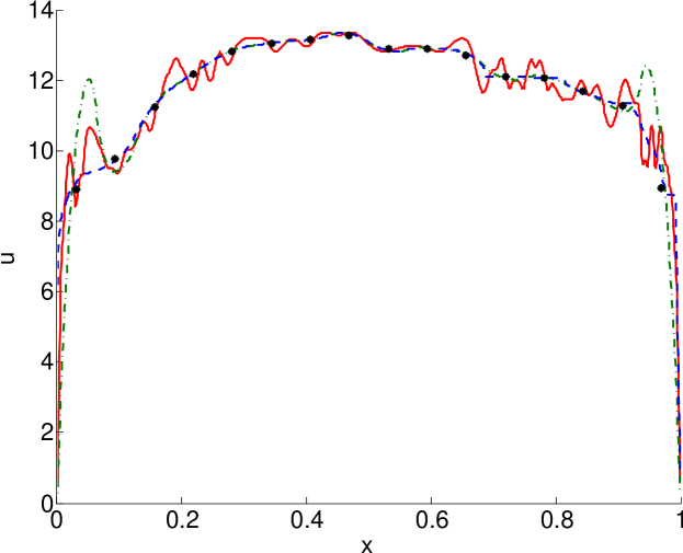
The algorithm produces artificial local extrema in areas of monotone large scale fields with large gradients, e.g. occurring near a wall as reported by McDermott (2005). Similar effects are known from deconvolution approaches within the fields of image and signal processing. We expand this algorithm by applying the linear slope limiter by Burbeau et al. (2001) after each recursive step in the area of monotone velocities. Hereby monotonicity is defined locally for one cell by including its neighbors.
Refer to caption
Figure 2: A representative instantaneous streamwise velocity profile u𝑢u (solid) for a turbulent channel (Reτ=1020𝑅subscript𝑒𝜏1020Re_{\tau}=1020) with NLES=16subscript𝑁LES16N_{\rm LES}=16 and NRSS=1024subscript𝑁RSS1024N_{\rm RSS}=1024 is shown. The large scale velocity uLES=[l]usuperscript𝑢LESdelimited-[]𝑙𝑢u^{\rm LES}=[l]u is represented with points. The deconvolution ua[l1]uLESsubscript𝑢𝑎delimited-[]superscript𝑙1superscript𝑢LESu_{a}\approx[l^{-1}]u^{\rm LES} using the original algorithm by Schmidt et al. (2008) is dashed-dotted and the limited algorithm is dashed. For both algorithms (limited and unlimited) the reconstructed field uasubscript𝑢𝑎u_{a} preserves the box-filtered values [l]ua=uLESdelimited-[]𝑙subscript𝑢𝑎superscript𝑢LES[l]u_{a}=u^{\rm LES}, but without the limiter unphysical overshoots occur near the walls.

The properties of the original algorithm and the limited one are demonstrated for a realistic instantaneous streamwise velocity profile u𝑢u for a turbulent channel case with high gradients at the walls, shown in Figure 2 (please note in XLES only large scale information is deconvolved).

The numerical deconvolution error due to the algorithm described can be written formally:

σ¯aspatial=(l¯¯C¯¯l¯¯aC¯¯)(xj(u¯^ju¯^iu¯¯jLESu¯¯iLES)+l¯¯2D¯ij).superscriptsubscript¯𝜎𝑎spatialsuperscript¯¯𝑙¯¯𝐶superscript¯¯𝑙subscript𝑎¯¯𝐶subscriptsubscript𝑥𝑗subscript^¯𝑢𝑗subscript^¯𝑢𝑖superscriptsubscript¯¯𝑢𝑗LESsuperscriptsubscript¯¯𝑢𝑖LESsuperscript¯¯𝑙2𝐷subscript¯𝑖𝑗\displaystyle{\underline{\sigma}}_{a}^{\rm spatial}=(\underline{\underline{l}}^{{\dagger}}*\underline{\underline{C}}-\underline{\underline{l}}^{{\dagger}_{a}}*\underline{\underline{C}})\left(\partial_{x_{j}}\left(\hat{\underline{u}}_{j}*\hat{\underline{u}}_{i}-\overline{\underline{u}}_{j}^{\rm LES}*\overline{\underline{u}}_{i}^{\rm LES}\right)+\underline{\underline{l}}^{2D}\mathcal{\underline{M}}_{ij}\right). (40)

There is no spectrally sharp way to implement this type of deconvolution. Various non-equivalent procedures are possible in principle. Schmidt et al. (2008) describe a particular approach that is adopted here with a technical modification that improves its behavior near walls. To summarize, although the inverse operator l1superscript𝑙1l^{-1} arises as a natural and necessary consequence of the XLES ansatz, the ansatz per se does not uniquely define its meaning nor guarantee that it can be specified in a way that is free of unintended artifacts.

3.2 XLES: Consistency Preservation and ‘LES limit’

Both, the XLES mass conservation in section 2.2.3 and the coupling terms in section 2.2.1 and 2.2.2 assume the 3D large scale velocity field to be consistent, meaning each XLES-grid k𝑘k contains the identical 3D large scale velocity field: u¯iLES=u¯k,iLES[lk]u^k,isuperscriptsubscript¯𝑢𝑖LESsuperscriptsubscript¯𝑢𝑘𝑖LESdelimited-[]subscript𝑙𝑘subscript^𝑢𝑘𝑖\overline{u}_{i}^{\rm LES}=\overline{u}_{k,i}^{\rm LES}\equiv[l_{k}]\hat{u}_{k,i}.

In the XLES-vector notation this condition can be written as:

l¯¯1Du¯^i=u¯¯iLES=u¯iLES(111)superscript¯¯𝑙1𝐷subscript^¯𝑢𝑖superscriptsubscript¯¯𝑢𝑖LESsuperscriptsubscript¯𝑢𝑖LESmatrix111\displaystyle\underline{\underline{l}}^{1D}\hat{\underline{u}}_{i}=\overline{\underline{u}}_{i}^{\rm LES}=\overline{{u}}_{i}^{\rm LES}\begin{pmatrix}1\\ 1\\ 1\end{pmatrix} (41)

with the 1D filter matrix defined in Eq. (11). This means consistency preserving terms should be independent of the XLES-grid k𝑘k.

We assume that the initial conditions are consistent (this can easily be achieved) and need to prove a consistency preserving XLES-advancement including advective and diffusive terms and the sub-grid modeling.

The ‘directly resolved’ advection terms themselves (xju¯^ju¯^jsubscriptsubscript𝑥𝑗subscript^¯𝑢𝑗subscript^¯𝑢𝑗\partial_{x_{j}}\hat{\underline{u}}_{j}*\hat{\underline{u}}_{j}) are violating the consistency condition, but by including the corresponding coupling (indirectly resolved terms): xju¯^ju¯^j+𝒳¯ijXLESsubscriptsubscript𝑥𝑗subscript^¯𝑢𝑗subscript^¯𝑢𝑗superscriptsubscript¯𝒳𝑖𝑗XLES\partial_{x_{j}}\hat{\underline{u}}_{j}*\hat{\underline{u}}_{j}+\mathcal{\underline{X}}_{ij}^{\rm XLES}, the consistency is preserved. The same is valid for microscale terms and their couplings: l¯¯2D¯ij+l¯¯aC¯¯l¯¯2D¯ijsuperscript¯¯𝑙2𝐷subscript¯𝑖𝑗superscript¯¯𝑙subscript𝑎¯¯𝐶superscript¯¯𝑙2𝐷subscript¯𝑖𝑗\underline{\underline{l}}^{2D}\mathcal{\underline{M}}_{ij}+\underline{\underline{l}}^{{\dagger}_{a}}*\underline{\underline{C}}\,\underline{\underline{l}}^{2D}\mathcal{\underline{M}}_{ij}.

By rearranging the XLES advection terms and their corresponding couplings, we find:

u¯^ju¯^i+𝒳¯ijXLES=u¯¯ju¯¯isubscript^¯𝑢𝑗subscript^¯𝑢𝑖superscriptsubscript¯𝒳𝑖𝑗XLESsubscript¯¯𝑢𝑗subscript¯¯𝑢𝑖\displaystyle\hat{\underline{u}}_{j}*\hat{\underline{u}}_{i}+\mathcal{\underline{X}}_{ij}^{\rm XLES}=\overline{\underline{u}}_{j}*\overline{\underline{u}}_{i} (42)

with u¯k,i=[l1l2l3+s1l2l3+l1s2l3+l1l2s3]uisubscript¯𝑢𝑘𝑖delimited-[]subscript𝑙1subscript𝑙2subscript𝑙3subscript𝑠1subscript𝑙2subscript𝑙3subscript𝑙1subscript𝑠2subscript𝑙3subscript𝑙1subscript𝑙2subscript𝑠3subscript𝑢𝑖\overline{u}_{k,i}=[l_{1}l_{2}l_{3}+s_{1}l_{2}l_{3}+l_{1}s_{2}l_{3}+l_{1}l_{2}s_{3}]u_{i}, which is equal in all XLES-grids k𝑘k.

The same holds for the XLES sub-grid terms l¯¯2D¯ijsuperscript¯¯𝑙2𝐷subscript¯𝑖𝑗\underline{\underline{l}}^{2D}\mathcal{\underline{M}}_{ij} and their corresponding couplings l¯¯aC¯¯l¯¯2D¯ijsuperscript¯¯𝑙subscript𝑎¯¯𝐶superscript¯¯𝑙2𝐷subscript¯𝑖𝑗\underline{\underline{l}}^{{\dagger}_{a}}*\underline{\underline{C}}\,\underline{\underline{l}}^{2D}\mathcal{\underline{M}}_{ij} (proof by insertion).

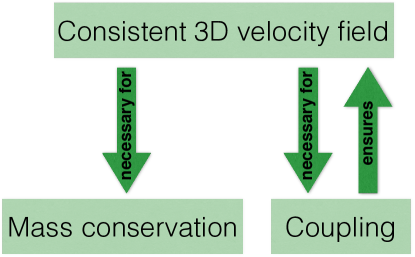
In consequence the coupling terms are essential for a consistent 3D velocity field within XLES, as illustrated in figure 3.
Refer to caption
Figure 3: On the one hand the consistency preservation is invoke before the advection step to define the coupling terms. On the other hand the coupling guarantees the consistency to be still preserved after the advection step.

In the implementation of XLES we check that the 3D large scale velocity field is still consistent every 100100100 timesteps to avoid numerical errors violating consistency preservation. All computations show the consistency to be limited by the floating point accuracy.

In the limit NRSSNLESsubscript𝑁RSSsubscript𝑁LESN_{\rm RSS}\rightarrow N_{\rm LES} the 2D filtered XLES-U equations collapse to the 3D filtered LES-U equations in each XLES-grid, because the RSS velocities vanish: uˇi=u^iu¯iLES=0subscriptˇ𝑢𝑖subscript^𝑢𝑖superscriptsubscript¯𝑢𝑖LES0\check{u}_{i}=\hat{u}_{i}-\overline{u}_{i}^{\rm LES}=0

For NLESNRSS(NDNS)subscript𝑁LESannotatedsubscript𝑁RSSabsentsubscript𝑁DNSN_{\rm LES}\rightarrow N_{\rm RSS}(\geq N_{\rm DNS}) in each direction, all velocity scales are resolved by the 3D grid and XLES-U (and LES-U) converges to DNS.

Within the ODT model, applied as an SGM in part II (Glawe et al. (2015)), all turbulent events are suppressed in the DNS-limit. Thus DNS is also a distinguished limit of ODTLES.

3.3 XLES: Coupled Advection Scheme

The characteristic shape of the XLES-grids (figure 1(b)1(d)) is considered when choosing the numerical schemes to be implemented, e.g. an implicit time discretization in the highly resolved direction is applied, while explicit time schemes are used to advect large scale properties. Therefore different numerical advection schemes are mixed due to the XLES coupling terms, because the same property, represented by several XLES-grids is simultaneously advanced by different numerical schemes. Additionally the coupling requires a deconvolution function, which interacts with these numerical schemes.

In this section we present the numerical properties of this coupled advection scheme. For simplicity the 3D large scale velocity fields u¯¯iLESsuperscriptsubscript¯¯𝑢𝑖LES\overline{\underline{u}}_{i}^{\rm LES} are resolved by NLESsubscript𝑁LESN_{\rm LES} cells in each direction. The resolved small scale (RSS) properties are discretized with NRSSsubscript𝑁RSSN_{\rm RSS} cells in all XLES-grids.

The coupled advection scheme numerically approximates the equation

0=0absent\displaystyle 0= (𝟙¯¯δi¯¯)(tu¯^i+j=13xju¯^ju¯^i+j=13(l¯¯C¯¯xj(u¯^ju¯^iu¯¯jLESu¯¯iLES)))¯¯double-struck-𝟙¯¯subscript𝛿𝑖subscript𝑡subscript¯^𝑢𝑖superscriptsubscript𝑗13subscriptsubscript𝑥𝑗subscript¯^𝑢𝑗subscript¯^𝑢𝑖superscriptsubscript𝑗13superscript¯¯𝑙¯¯𝐶subscriptsubscript𝑥𝑗subscript^¯𝑢𝑗subscript^¯𝑢𝑖superscriptsubscript¯¯𝑢𝑗LESsuperscriptsubscript¯¯𝑢𝑖LES\displaystyle(\underline{\underline{\mathbb{1}}}-\underline{\underline{\delta_{i}}})\left(\partial_{t}\underline{\hat{u}}_{i}+\sum_{j=1}^{3}\partial_{x_{j}}\underline{\hat{u}}_{j}*\underline{\hat{u}}_{i}+\sum_{j=1}^{3}\left(\underline{\underline{l}}^{{\dagger}}*\underline{\underline{C}}\partial_{x_{j}}(\hat{\underline{u}}_{j}*\hat{\underline{u}}_{i}-\overline{\underline{u}}_{j}^{\rm LES}*\overline{\underline{u}}_{i}^{\rm LES})\right)\right) (43)

(according to Eq. (38); SGS terms are not considered).

Fundamental properties of the coupled advection scheme, e.g. the numerical dissipation and dispersion, can be demonstrated by solving a one dimensional linear advection problem. Then a constant wave speed cjsubscript𝑐𝑗c_{j} replaces the advecting velocities in Eq. (43): u¯^j=u¯¯jLES=cj(111)Tsubscript¯^𝑢𝑗superscriptsubscript¯¯𝑢𝑗LESsubscript𝑐𝑗superscriptmatrix111𝑇\underline{\hat{u}}_{j}=\overline{\underline{u}}_{j}^{\rm LES}=c_{j}\begin{pmatrix}1&1&1\end{pmatrix}^{T}. In this section the linearized coupled advection scheme is investigated, while the full non-linear coupled advection scheme is studied in section 3.4.

W.l.o.g. the advected velocity u¯1subscript¯𝑢1{\underline{u}}_{1} is represented by the two staggered XLES-grids containing u^2,1subscript^𝑢21\hat{{u}}_{{2,1}} and u^3,1subscript^𝑢31\hat{{u}}_{{3},1} respectively while u^1,1subscript^𝑢11\hat{{u}}_{1,1} is evaluated using Eq. (36).

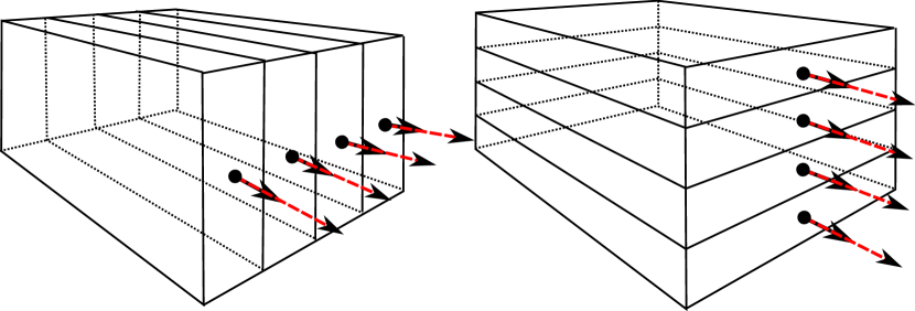
Two situations occur (see figure 4), as discussed here by a concrete example (generalization to other indices is trivial):
  • 1.

    Case 111: j=i=w.l.o.g.1j=i\stackrel{{\scriptstyle w.l.o.g.}}{{=}}1 in Eq. (43): Advection into x1subscript𝑥1x_{1}-direction; In both XLES-grids 22{2} and 33{3} the advection is coarsely resolved with NLESsubscript𝑁LESN_{\rm LES} grid cells.

  • 2.

    Case 222: 2=w.l.o.g.ji=w.l.o.g.12\stackrel{{\scriptstyle w.l.o.g.}}{{=}}j\neq i\stackrel{{\scriptstyle w.l.o.g.}}{{=}}1 in Eq. (43): Advection into direction x2subscript𝑥2x_{2}; In XLES-grid 222 the advection is resolved with NRSSsubscript𝑁RSSN_{\rm RSS} cells, respective with NLESsubscript𝑁LESN_{\rm LES} cells in XLES-grid 33{3}.

Refer to caption
(a) Case 111: j=i𝑗𝑖j=i in Eq. (43). Coarsely resolved advection in XLES-grid 333 (left) and XLES-grid 222 (right).
Refer to caption
(b) Case 222: ji𝑗𝑖j\neq i in Eq. (43). Highly (coarsely) resolved advection in XLES-grid 333 (left) (XLES-grid 222 (right)).
Figure 4: XLES requires a coupled advection scheme. The advected velocity u¯^isubscript^¯𝑢𝑖\hat{\underline{u}}_{i} (bold arrows) is advected with the constant wave speed cjsubscript𝑐𝑗c_{j} (dashed arrows) and is resolved in two XLES-grids. For the two relevant cases the discrete staggered grids within one 3D large scale cell (compare to figure 1) are shown in (a) and (b).

To spatially discretize the advection terms, a central difference method (CDM) on a staggered grid is used.

Two different time discretizations are deployed:

  • 1.

    The highly resolved properties (using NRSSsubscript𝑁RSSN_{\rm RSS} cells) are discretized using a standard 2nd2𝑛𝑑2nd order Crank-Nicolson (CN) scheme in time (see Crank and Nicolson (1996)). We will refer to this fully discrete scheme as CN-CDM.

  • 2.

    The coarse grained resolved properties (using NLESsubscript𝑁LESN_{\rm LES} cells) are discretized using a 333-stage 3rd3𝑟𝑑3rd order TVD Runge-Kutta (RK3) scheme (see Spiteri and Ruuth (2002)). We will refer to this fully discrete scheme as RK3-CDM

The numerical properties of the numerical schemes without coupling are:

  • 1.

    The advection scheme CN-CDM is stable, dissipation free and has low dispersion.

  • 2.

    The RK3-CDM scheme is found to be stable, producing little dispersion and dissipation.

These properties transfer to the coupled advection schemes (in Cases 111 and 222).

Based on the expressions RK3-CDM and CN-CDM the coupled advection scheme in Case 111 (Case 222) is called RK3-RK3-CDM (CN-RK3-CDM).

To illustrate the coupling procedure w.l.o.g. for the CN-RK3-CDM scheme, we linearize and rewrite Eq. (43) in a semi-discrete form (in index notation). Hereby u^3,1subscript^𝑢31\hat{u}_{3,1} is discretized in XLES-grid 333 in Eq. (44) and u^2,1subscript^𝑢21\hat{u}_{2,1} in XLES-grid 222 in Eq. (45):

(Δt)u^3,1=Δ𝑡subscript^𝑢31absent\displaystyle(\Delta t)\hat{u}_{3,1}= RK3c2x2u^3,1dtsubscript𝑅𝐾3subscript𝑐2subscriptsubscript𝑥2subscript^𝑢31d𝑡\displaystyle\int_{RK3}c_{2}\partial_{x_{2}}{\hat{u}_{3,1}}{\rm\,d}t (44)
+[l31][l2](CNc2x2u^2,1dtRK3c2x2u¯2,1LESdt)delimited-[]superscriptsubscript𝑙31delimited-[]subscript𝑙2subscript𝐶𝑁subscript𝑐2subscriptsubscript𝑥2subscript^𝑢21d𝑡subscript𝑅𝐾3subscript𝑐2subscriptsubscript𝑥2superscriptsubscript¯𝑢21LESd𝑡\displaystyle+[l_{3}^{-1}][l_{2}]\left(\int_{CN}c_{2}\partial_{x_{2}}\hat{{u}}_{2,1}{\rm\,d}t-\int_{RK3}c_{2}\partial_{x_{2}}\overline{{u}}_{2,1}^{\rm LES}{\rm\,d}t\right)
(Δt)u^2,1=Δ𝑡subscript^𝑢21absent\displaystyle(\Delta t)\hat{u}_{2,1}= CNc2x2u^2,1dtsubscript𝐶𝑁subscript𝑐2subscriptsubscript𝑥2subscript^𝑢21d𝑡\displaystyle\int_{CN}c_{2}\partial_{x_{2}}{\hat{u}_{2,1}}{\rm\,d}t (45)
+[l21][l3](RK3c2x2u^3,1dtRK3c2x2u¯3,1LESdt).delimited-[]superscriptsubscript𝑙21delimited-[]subscript𝑙3subscript𝑅𝐾3subscript𝑐2subscriptsubscript𝑥2subscript^𝑢31d𝑡subscript𝑅𝐾3subscript𝑐2subscriptsubscript𝑥2superscriptsubscript¯𝑢31LESd𝑡\displaystyle+[l_{2}^{-1}][l_{3}]\left(\int_{RK3}c_{2}\partial_{x_{2}}\hat{{u}}_{3,1}{\rm\,d}t-\int_{RK3}c_{2}\partial_{x_{2}}\overline{{u}}_{3,1}^{\rm LES}{\rm\,d}t\right).

Here the numerical time discretizations of the advection terms are indicated (CN and RK3). The discrete coupling operators [lk]delimited-[]subscript𝑙𝑘[l_{k}] and [lk1]delimited-[]superscriptsubscript𝑙𝑘1[l_{k}^{-1}] (see Eq. (7) and the algorithm described in section 3.1) are discretized by an explicit Euler scheme in time. Also the non-linear advection part which is not considered in the linear advection problem is discretized by an explicit Euler scheme in time.

The properties of the fully discrete linear coupled advection schemes are:

  • 1.

    The coupled advection scheme converges to the analytical solution for NLESsubscript𝑁LESN_{\rm LES}\rightarrow\infty as investigated in C.2 where the theoretical prediction e.g. by Tsai et al. (2002) is reproduced. This property is required to numerically realize the LES limit and DNS limit of XLES (section 3.2).

  • 2.

    The coupled advection scheme including the deconvolution (see section 3.1) reproduces well defined large scale behavior, even by simultaneously transporting small scale properties, as investigated in C.3.

The highly resolved CN-CDM scheme (using NRSSsubscript𝑁RSSN_{\rm RSS} cells) contributes to the coupled CN-RK3-CDM scheme (Case 222) and additionally increases the numerical accuracy of the coupled scheme. This is neither required for a well defined and converging XLES scheme nor the LES limit (or DNS limit) of XLES. As investigated in C.2 the highly resolved advection terms increase the coupled numerical accuracy up to a resolution ratio NRSS/NLES10less-than-or-similar-tosubscript𝑁RSSsubscript𝑁LES10{N_{\rm RSS}/N_{\rm LES}}\lesssim 10. With NRSS10NLESgreater-than-or-equivalent-tosubscript𝑁RSS10subscript𝑁LESN_{\rm RSS}\gtrsim 10N_{\rm LES} the overall numerical error is dominated by the coarsely resolved RK3-CDM scheme.

The coupled numerical schemes, simultaneously discretized by multiple XLES-grids, are found to be appropriate for linear advection. Important numerical properties, like stability and dissipative behavior, transfer from the well known underlying numerical discretizations to the coupled advection scheme.

There are other time schemes, that possibly can be adapted to the special requirements of the XLES time advancement, e.g.:

  • 1.

    An IMEX (implicit/explicit) time scheme (see e.g. Cavaglieri and Bewley (2015) and references cited therein) applied to XLES can in principle lead to a high-order time integration for all terms (including non-linear advection and coupling), but to include the coupling terms into such a high order time scheme requires identical coefficients for the implicit and explicit integration terms.

  • 2.

    Adapting split-explicit schemes (see e.g. Gadd (1978)) to the XLES coupled advection can especially decrease the dispersive effects that arise.

  • 3.

    Large time step wave propagation schemes based on the work by LeVeque (1985) can perhaps improve the numerical properties of the applied CN scheme within the XLES advection scheme.

For the sake of completeness the diffusion terms are discretized by a central difference scheme in space with a first order explicit (implicit) Euler scheme in the coarse (fine) resolved XLES-grid direction.

3.4 XLES: Convergence of the XLES Approach

To verify the XLES model, we conduct a convergence study of XLES-U (unclosed XLES) for a fully developed turbulent flow, including the full diversity of non-linear advective effects: A turbulent channel flow with a friction Reynolds number Reτ=395𝑅subscript𝑒𝜏395Re_{\tau}=395 is computed. DNS results by Kawamura et al. (1999) (online available: Kawamura (2014)) are compared to the XLES-U outcome.

The DNS is resolved with NDNS=192subscript𝑁𝐷𝑁𝑆192N_{DNS}=192 non-equidistant cells in the horizontal direction (between the walls). For the spatial discretization a second order central difference scheme is used. The time is discretized using a Crank-Nicolson scheme for the wall-normal non-linear terms and a second order Adams-Bashforth scheme for other terms (results for higher resolutions and higher order schemes are also available online). This numerical scheme is comparable to the XLES-U numerical scheme (see section 3.3).

For the XLES-U convergence study, the number of equidistant 3D large scale cells NLESsubscript𝑁LESN_{\rm LES} is increased using the values NLES={16,32,64}subscript𝑁LES163264N_{\rm LES}=\{16,32,64\} while NRSS=512subscript𝑁RSS512N_{\rm RSS}=512 is kept constant.

The time step size is limited by:

Δt=CFLmini,k(Δxk,iRSSu^k,i),i,k={1,2,3}formulae-sequenceΔ𝑡𝐶𝐹𝐿subscript𝑖𝑘Δsuperscriptsubscript𝑥𝑘𝑖RSSsubscript^𝑢𝑘𝑖𝑖𝑘123\displaystyle\Delta t=CFL\,\min_{i,k}\left(\frac{\Delta x_{k,i}^{\rm RSS}}{\hat{u}_{k,i}}\right),\,i,k=\{1,2,3\} (46)

with a Courant-Friedrichs-Lewy number CFL=0.45𝐶𝐹𝐿0.45CFL=0.45 and the small scale cell size Δxk,iRSSΔsuperscriptsubscript𝑥𝑘𝑖RSS\Delta x_{k,i}^{\rm RSS}.

To produce statistically significant results, the flow is averaged for tave25subscript𝑡𝑎𝑣𝑒25t_{ave}\geq 25 non-dimensional time units (compared to tave=20subscript𝑡𝑎𝑣𝑒20t_{ave}=20 for DNS) after reaching a statistically steady state.

Additionally equidistant discretized LES-U (LES limit of XLES-U with NRSS=NLESsubscript𝑁RSSsubscript𝑁LESN_{\rm RSS}=N_{\rm LES}, see section 3.2) channel flow results are compared to XLES-U. The latter resolves selected advective and diffusive small scale effects even without using a SGM. Those can be identified by comparing the XLES-U and LES-U channel flow results.

Figure 5 illustrates the results: The mean velocity profiles computed by XLES-U (see figure 5(b)) and LES-U (see figure 5(a)) are compared to DNS.

Additionally the streamwise and spanwise velocity RMSs (see figure 5(c)) and the budget terms of the turbulent kinetic energy (see figure 5(d)- 5(f)) are shown for XLES-U, LES-U, and DNS.
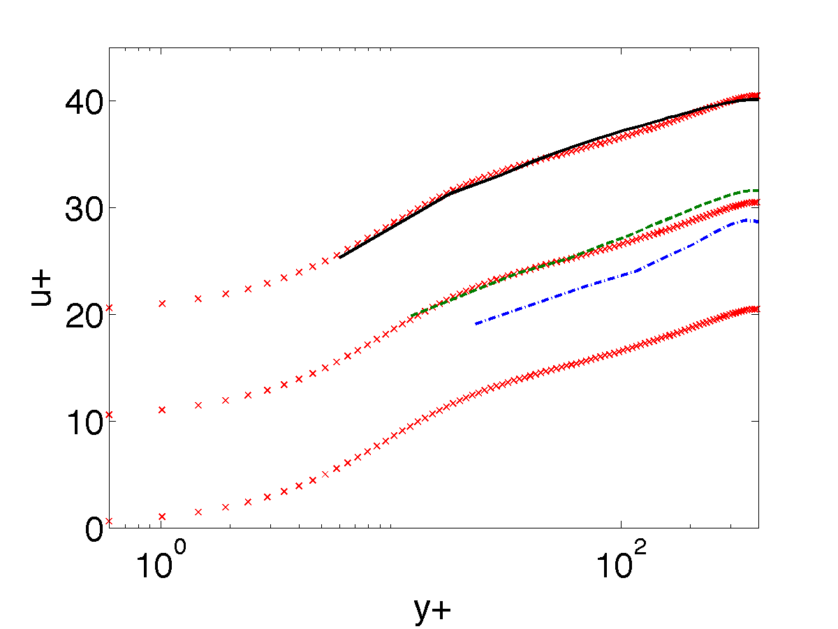
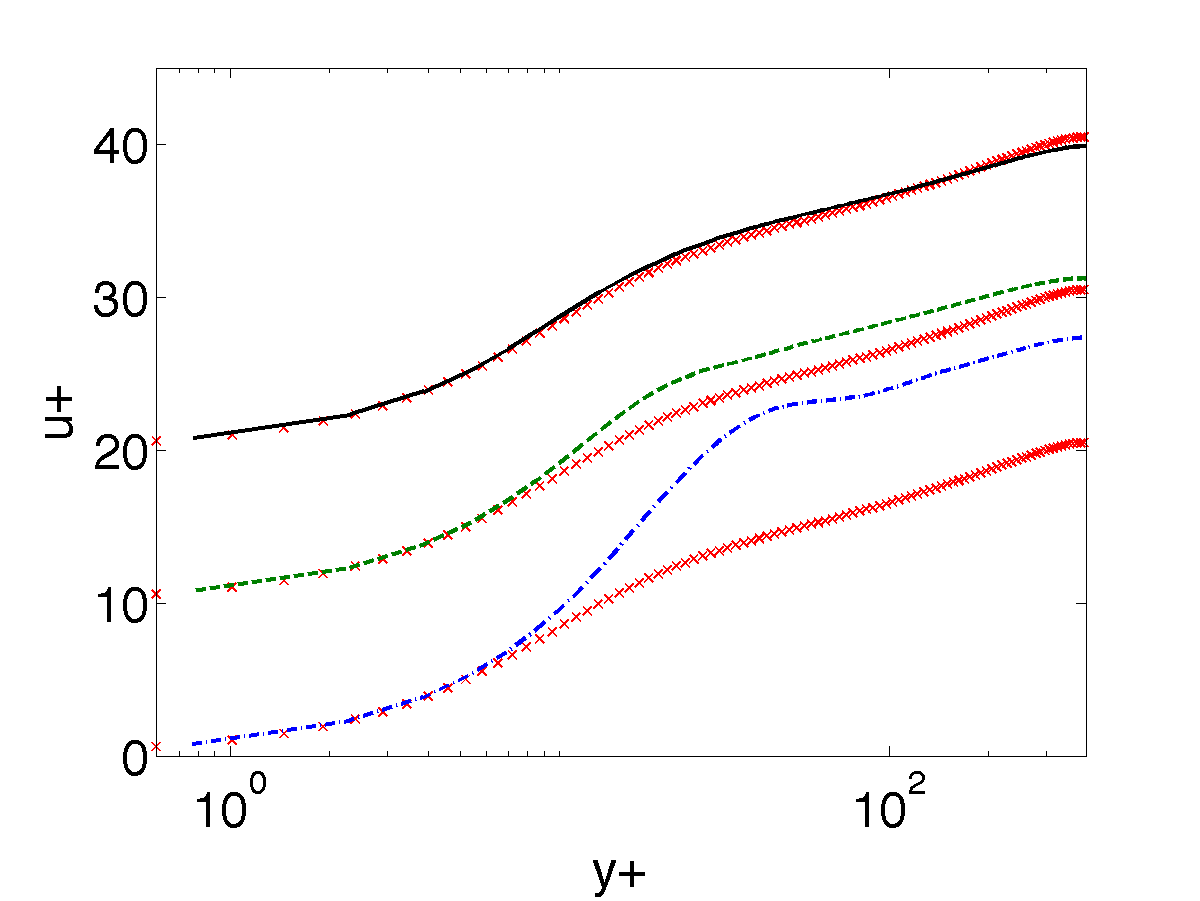
Refer to caption
(a) LES: law of the wall (u¯1LESsuperscriptsubscript¯𝑢1LES\overline{u}_{1}^{\rm LES}). Profiles shifted with increasing NLESsuperscript𝑁LESN^{\rm LES}.
Refer to caption
(b) XLES: law of the wall (u^2,1subscript^𝑢21\hat{u}_{2,1}). Profiles shifted with increasing NLESsuperscript𝑁LESN^{\rm LES}.
Refer to caption
(c) Streamwise (uRMSsubscript𝑢RMSu_{\rm RMS}) and spanwise (wRMSsubscript𝑤RMSw_{\rm RMS}) velocity RMS.
Refer to caption
(d) Production (Prod) and Dissipation (Diss) of the turbulent kinetic energy.
Refer to caption
(e) Viscous transport of the turbulent kinetic energy (tv).
Refer to caption
(f) Advective transport of the turbulent kinetic energy (ta).
Figure 5: Turbulent channel flow results for DNS (small crosses), LES-U, and XLES-U with NLES=16subscript𝑁LES16N_{\rm LES}=16 (dash-dotted), NLES=32subscript𝑁LES32N_{\rm LES}=32 (dashed), and NLES=64subscript𝑁LES64N_{\rm LES}=64 (solid). The XLES-U small scales are resolved using NRSS=512subscript𝑁RSS512N_{\rm RSS}=512 cells. XLES-U mean and statistical flow properties are based on the velocity field perpendicular to the channel walls u^2,isubscript^𝑢2𝑖\hat{u}_{2,i} (in the LES limit: u^2,i=u¯iLESsubscript^𝑢2𝑖superscriptsubscript¯𝑢𝑖LES\hat{u}_{2,i}=\overline{u}_{i}^{\rm LES}).

Both XLES-U and LES-U show convergence towards the DNS results with increasing 3D resolution. Following arguments in section 3.2 this implies the XLES error term σ¯XLESspatialsuperscriptsubscript¯𝜎𝑋𝐿𝐸𝑆spatial{\underline{\sigma}}_{XLES}^{\rm spatial} to be small. Additionally the XLES non-linear terms (and its LES limit) are sufficiently represented and converging, even if the under-resolved velocity profile (figure 5(a) and 5(b)) indicates noticeable numerical dissipation.

XLES-U is able to accurately represent diffusive effects, e.g. the laminar sublayer near the walls, independent of the 3D large scale resolution and reproduces basic advective effects including turbulence with NLES32greater-than-or-equivalent-tosubscript𝑁LES32N_{\rm LES}\gtrsim 32 3D cells for Reτ=395𝑅subscript𝑒𝜏395Re_{\tau}=395. Additionally the turbulence statistics profit from the additional small scale effects represented by XLES compared to LES-U even with low 3D resolutions.

In part II (Glawe et al. (2015)) ODT is demonstrated to represent the turbulent effects not resolved by XLES-U, even with very coarse 3D resolutions (e.g. NLES=16subscript𝑁LES16N_{\rm LES}=16).

4 Conclusions

In this work XLES, an extended LES model, is introduced. This approach is intended as a basis for a new class of turbulence models, tailored to describe a (XLES specific) macrostructure of highly turbulent flows including fully resolved molecular diffusion in domains of moderate complexity.

An innovative XLES filter strategy is derived, including a numerical representation of the resulting 2D filtered XLES equations by three coupled XLES-grids. This coupling requires a high order deconvolution function for 1D box filtered fields, wherefore a stabilized version of the algorithm introduced by Schmidt et al. (2008) is applied.

The 3D filtered LES-U (unclosed LES) equations and DNS are distinguished limits of XLES-U (unclosed XLES).

We verify the XLES-U equations:

  • 1.

    By analyzing the coupled (linear) advection scheme occurring in XLES.

  • 2.

    By performing a convergence study: The turbulent channel flow with Reτ=395𝑅subscript𝑒𝜏395Re_{\tau}=395 is compared to DNS and LES-U. Compared to LES-U low 3D resolutions are required in XLES-U to reproduce fundamental flow statistics, especially in the near wall region. E.g. the laminar sublayer is fully represented independently of the 3D resolution.

An XLES closure can be provided by the ODT model, which is able to capture the full turbulent cascade of highly turbulent flows, as introduced in part II (Glawe et al. (2015)). Recently Meiselbach (2015) introduces channel flow results up to Reτ=600000𝑅subscript𝑒𝜏600000Re_{\tau}=600000 using adaptive ODT by Lignell et al. (2013). This ODTLES model enables the representation of highly turbulent flows in domains of moderate complexity with coarse 3D resolutions basically independent of turbulent scales and at once represents diffusive and (turbulent) advective effects down to the molecular level using ODT. Hereby the 3D resolution needs to be sufficient to resolve the domain and possible secondary effects. E.g. due to secondary instabilities within a duct flow, the 3D resolution indirectly depends on the Reynolds number (investigated in part II by Glawe et al. (2015)). The XLES model is especially advantageous for turbulent flows with crucial small scale effects, e.g. with important Prandtl or Schmidt number effects, buoyant stratification effects, or in the field of combustion.

In XLES a potential bottleneck in highly resolved incompressible simulations, the pressure handling, is only computed on a very coarse 3D grid and small scale pressure effects might be modeled. Closed XLES (e.g. ODTLES) is a promising and highly parallelizable approach to investigate fundamental atmospheric turbulent flows.

Acknowledgments

The authors would like to thank H. Kawamura and colleagues for providing DNS results online (Kawamura (2014)). This work was supported by the Brandenburg University of Technology Cottbus-Senftenberg, the Helmholtz graduate research school GeoSim, and the Freie Universität Berlin.

Appendix A XLES: Vector Notation

We introduce an alternative to the vector notation in section 2 by writing the XLES velocity scales in index notation. The XLES vector u¯^isubscript^¯𝑢𝑖\hat{\underline{u}}_{i} includes the XLES vector elements u^k,isubscript^𝑢𝑘𝑖\hat{{u}}_{k,i} represented in XLES-grids k𝑘k, k={1,2,3}𝑘123k=\{1,2,3\}.

In index notation the resolved small scale (RSS) terms s1l2l3subscript𝑠1subscript𝑙2subscript𝑙3s_{1}l_{2}l_{3}, l1s2l3subscript𝑙1subscript𝑠2subscript𝑙3l_{1}s_{2}l_{3}, and l1l2s3subscript𝑙1subscript𝑙2subscript𝑠3l_{1}l_{2}s_{3} can be expressed by one term: sklk1ll2subscript𝑠𝑘subscript𝑙direct-sum𝑘1subscript𝑙direct-sum𝑙2s_{k}l_{k\oplus 1}l_{l\oplus 2}, where {k,k1,k2}𝑘direct-sum𝑘1direct-sum𝑘2\{k,k\oplus 1,k\oplus 2\} is a positive permutation of {1,2,3}123\{1,2,3\} (the 1D filter operators are commutable). The operator direct-sum\oplus denotes the positive permutation:

qx=((q+x1)mod3)+2direct-sum𝑞𝑥modulo𝑞𝑥132\displaystyle q\oplus x=((q+x-1)\mod 3)+2 (47)

for q={1,2,3}𝑞123q=\{1,2,3\} and x={1,2}𝑥12x=\{1,2\} (valid in three dimensions).

The XLES resolved velocity scales (Eq. (12)) are written in index notation (using the operator direct-sum\oplus):

u¯isubscript¯𝑢𝑖\displaystyle\overline{u}_{i} =[l1l2l3+s1l2l3+l1s2l3+l1l2s3]uiabsentdelimited-[]subscript𝑙1subscript𝑙2subscript𝑙3subscript𝑠1subscript𝑙2subscript𝑙3subscript𝑙1subscript𝑠2subscript𝑙3subscript𝑙1subscript𝑙2subscript𝑠3subscript𝑢𝑖\displaystyle=\left[{l_{1}l_{2}l_{3}+s_{1}l_{2}l_{3}+l_{1}s_{2}l_{3}+l_{1}l_{2}s_{3}}\right]u_{i}
=\displaystyle= [l1l2l3+q=13sqlq1lq2]uidelimited-[]subscript𝑙1subscript𝑙2subscript𝑙3superscriptsubscript𝑞13subscript𝑠𝑞subscript𝑙direct-sum𝑞1subscript𝑙direct-sum𝑞2subscript𝑢𝑖\displaystyle\left[l_{1}l_{2}l_{3}+\sum_{q=1}^{3}s_{q}l_{q\oplus 1}l_{q\oplus 2}\right]u_{i} (48)
=\displaystyle= [q=13(lqlq1lq2+sqlq1lq2)2l1l2l3]ui.delimited-[]superscriptsubscript𝑞13subscript𝑙𝑞subscript𝑙direct-sum𝑞1subscript𝑙direct-sum𝑞2subscript𝑠𝑞subscript𝑙direct-sum𝑞1subscript𝑙direct-sum𝑞22subscript𝑙1subscript𝑙2subscript𝑙3subscript𝑢𝑖\displaystyle\left[\sum_{q=1}^{3}\left(l_{q}l_{q\oplus 1}l_{q\oplus 2}+s_{q}l_{q\oplus 1}l_{q\oplus 2}\right)-2l_{1}l_{2}l_{3}\right]u_{i}.

The 3D large scale operator [l1l2l3]delimited-[]subscript𝑙1subscript𝑙2subscript𝑙3[l_{1}l_{2}l_{3}] in the last row of Eq. (48) can be expressed in terms of [lqlq1lq2+sqlq1lq2]delimited-[]subscript𝑙𝑞subscript𝑙direct-sum𝑞1subscript𝑙direct-sum𝑞2subscript𝑠𝑞subscript𝑙direct-sum𝑞1subscript𝑙direct-sum𝑞2[l_{q}l_{q\oplus 1}l_{q\oplus 2}+s_{q}l_{q\oplus 1}l_{q\oplus 2}]:

2l1l2l3=2subscript𝑙1subscript𝑙2subscript𝑙3absent\displaystyle-2l_{1}l_{2}l_{3}= q=13(1δqk)(lqlq1lq2)superscriptsubscript𝑞131subscript𝛿𝑞𝑘subscript𝑙𝑞subscript𝑙direct-sum𝑞1subscript𝑙direct-sum𝑞2\displaystyle-\sum_{q=1}^{3}(1-\delta_{qk})(l_{q}l_{q\oplus 1}l_{q\oplus 2})
=\displaystyle= q=13(1δqk)((lqlq+lqlqlq)lq1lq2)superscriptsubscript𝑞131subscript𝛿𝑞𝑘subscript𝑙𝑞subscript𝑙𝑞subscript𝑙𝑞subscript𝑙𝑞subscript𝑙𝑞subscript𝑙direct-sum𝑞1subscript𝑙direct-sum𝑞2\displaystyle-\sum_{q=1}^{3}(1-\delta_{qk})((l_{q}l_{q}+l_{q}-l_{q}l_{q})l_{q\oplus 1}l_{q\oplus 2}) (49)
=\displaystyle= q=13(1δqk)lq(lqlq1lq2+(1lq)=sqlq1lq2)superscriptsubscript𝑞131subscript𝛿𝑞𝑘subscript𝑙𝑞subscript𝑙𝑞subscript𝑙direct-sum𝑞1subscript𝑙direct-sum𝑞2subscript1subscript𝑙𝑞absentsubscript𝑠𝑞subscript𝑙direct-sum𝑞1subscript𝑙direct-sum𝑞2\displaystyle-\sum_{q=1}^{3}(1-\delta_{qk})l_{q}(l_{q}l_{q\oplus 1}l_{q\oplus 2}+\underbrace{(1-l_{q})}_{=s_{q}}l_{q\oplus 1}l_{q\oplus 2})

with the Kronecker delta operator defined in Eq. (37).

Here an additional arbitrary index k={1,2,3}𝑘123k=\{1,2,3\} is introduced. Eq. (49) is satisfied for k=1𝑘1k=1, k=2𝑘2k=2, and k=3𝑘3k=3. This index k𝑘k spans the XLES vector.

Insertion of the 3D large scale operator (Eq. (49)) into the XLES resolved velocity scales (Eq. (48)) leads to:

u¯k,isubscript¯𝑢𝑘𝑖\displaystyle\overline{u}_{k,i} =[q=13(1(lqlqδqk))(lqlq1lq2+sqlq1lq2)]ui,k={1,2,3}.formulae-sequenceabsentdelimited-[]superscriptsubscript𝑞131subscript𝑙𝑞subscript𝑙𝑞subscript𝛿𝑞𝑘subscript𝑙𝑞subscript𝑙direct-sum𝑞1subscript𝑙direct-sum𝑞2subscript𝑠𝑞subscript𝑙direct-sum𝑞1subscript𝑙direct-sum𝑞2subscript𝑢𝑖𝑘123\displaystyle=\left[\sum_{q=1}^{3}(1-(l_{q}-l_{q}\delta_{qk}))\left(l_{q}l_{q\oplus 1}l_{q\oplus 2}+s_{q}l_{q\oplus 1}l_{q\oplus 2}\right)\right]u_{i},\;k=\{1,2,3\}. (50)

This XLES resolved velocity u¯k,isubscript¯𝑢𝑘𝑖\overline{u}_{k,i} reproduces exactly the XLES resolved velocity scales in Eq. (12) including the XLES coupling C¯¯s¯¯1Dl¯¯2D¯¯𝐶superscript¯¯𝑠1𝐷superscript¯¯𝑙2𝐷\underline{\underline{C}}\,\underline{\underline{s}}^{1D}\underline{\underline{l}}^{2D}. XLES is interpreted as approach filtering the Navier-Stokes equations by applying the operator [l1l2l3+s1l2l3+l1s2l3+l1l2s3]delimited-[]subscript𝑙1subscript𝑙2subscript𝑙3subscript𝑠1subscript𝑙2subscript𝑙3subscript𝑙1subscript𝑠2subscript𝑙3subscript𝑙1subscript𝑙2subscript𝑠3\left[{l_{1}l_{2}l_{3}+s_{1}l_{2}l_{3}+l_{1}s_{2}l_{3}+l_{1}l_{2}s_{3}}\right] compared to [l1l2l3]delimited-[]subscript𝑙1subscript𝑙2subscript𝑙3\left[{l_{1}l_{2}l_{3}}\right] in LES (see table 1).

Appendix B XLES Mass Conservation: Resolved Small Scales

Divergence-free XLES velocity fields u¯^isubscript^¯𝑢𝑖\hat{\underline{u}}_{i} are guaranteed, if the 3D large scale velocity field u¯¯iLES=[lk]u^k,isuperscriptsubscript¯¯𝑢𝑖𝐿𝐸𝑆delimited-[]subscript𝑙𝑘subscript^𝑢𝑘𝑖\overline{\underline{u}}_{i}^{LES}=[l_{k}]\hat{u}_{k,i} fulfills three conditions (see section 2.2.3):

  • 1.

    Con.111: u¯k,iLESsuperscriptsubscript¯𝑢𝑘𝑖𝐿𝐸𝑆\overline{u}_{k,i}^{LES} is consistent (u¯iLES=u¯k,iLESsuperscriptsubscript¯𝑢𝑖𝐿𝐸𝑆superscriptsubscript¯𝑢𝑘𝑖𝐿𝐸𝑆\overline{u}_{i}^{LES}=\overline{u}_{k,i}^{LES})

  • 2.

    Con.222: u¯iLESsuperscriptsubscript¯𝑢𝑖𝐿𝐸𝑆\overline{u}_{i}^{LES} is divergence free, enforced by 3D standard approach.

  • 3.

    Con.333: [lk]delimited-[]subscript𝑙𝑘[l_{k}] is a discrete 1D box filter (defined in Eq. (7)) in xksubscript𝑥𝑘x_{k}-direction.

The XLES velocity fields u¯^isubscript^¯𝑢𝑖\hat{\underline{u}}_{i} are divergence free as proved within one 3D large scale cell of the size ΔxkΔsubscript𝑥𝑘\Delta{x_{k}} in xksubscript𝑥𝑘x_{k}-direction (operator direct-sum\oplus is defined in Eq. (47)):

00\displaystyle 0 =Δxk2Δxk2j=13xj(u¯k,jLES+uˇk,j)dxk=Δxk2Δxk2j=13xju^k,jdxkabsentsuperscriptsubscriptΔsubscript𝑥𝑘2Δsubscript𝑥𝑘2superscriptsubscript𝑗13subscriptsubscript𝑥𝑗superscriptsubscript¯𝑢𝑘𝑗LESsubscriptˇ𝑢𝑘𝑗dsubscript𝑥𝑘superscriptsubscriptΔsubscript𝑥𝑘2Δsubscript𝑥𝑘2superscriptsubscript𝑗13subscriptsubscript𝑥𝑗subscript^𝑢𝑘𝑗dsubscript𝑥𝑘\displaystyle=\int_{-\frac{\Delta x_{k}}{2}}^{\frac{\Delta x_{k}}{2}}\sum_{j=1}^{3}\partial_{x_{j}}(\overline{u}_{k,j}^{\rm LES}+\check{u}_{k,j}){\rm\,d}x_{k}=\int_{-\frac{\Delta x_{k}}{2}}^{\frac{\Delta x_{k}}{2}}\sum_{j=1}^{3}\partial_{x_{j}}\hat{u}_{k,j}{\rm\,d}x_{k} (51)
=Δxk2Δxk2xku^k,kdxk+Δxk2Δxk2xk1u^k,k1dxk+Δxk2Δxk2xk2u^k,k2dxkabsentsuperscriptsubscriptΔsubscript𝑥𝑘2Δsubscript𝑥𝑘2subscriptsubscript𝑥𝑘subscript^𝑢𝑘𝑘dsubscript𝑥𝑘superscriptsubscriptΔsubscript𝑥𝑘2Δsubscript𝑥𝑘2subscriptsubscript𝑥direct-sum𝑘1subscript^𝑢𝑘direct-sum𝑘1dsubscript𝑥𝑘superscriptsubscriptΔsubscript𝑥𝑘2Δsubscript𝑥𝑘2subscriptsubscript𝑥direct-sum𝑘2subscript^𝑢𝑘direct-sum𝑘2dsubscript𝑥𝑘\displaystyle=\int_{-\frac{\Delta x_{k}}{2}}^{\frac{\Delta x_{k}}{2}}\partial_{x_{k}}\hat{{u}}_{k,k}{\rm\,d}{x_{k}}+\int_{-\frac{\Delta x_{k}}{2}}^{\frac{\Delta x_{k}}{2}}\partial_{x_{k\oplus 1}}\hat{u}_{k,{k\oplus 1}}{\rm\,d}{x_{k}}+\int_{-\frac{\Delta x_{k}}{2}}^{\frac{\Delta x_{k}}{2}}\partial_{x_{k\oplus 2}}\hat{{u}}_{k,{k\oplus 2}}{\rm\,d}{x_{k}}
=u^k,k(Δxk2)u^k,k(Δxk2)+xk1Δxk2Δxk2u^k,k1dxk+xk2Δxk2Δxk2u^k,k2dxkabsentsubscript^𝑢𝑘𝑘Δsubscript𝑥𝑘2subscript^𝑢𝑘𝑘Δsubscript𝑥𝑘2subscriptsubscript𝑥direct-sum𝑘1superscriptsubscriptΔsubscript𝑥𝑘2Δsubscript𝑥𝑘2subscript^𝑢𝑘direct-sum𝑘1differential-dsubscript𝑥𝑘subscriptsubscript𝑥direct-sum𝑘2superscriptsubscriptΔsubscript𝑥𝑘2Δsubscript𝑥𝑘2subscript^𝑢𝑘direct-sum𝑘2differential-dsubscript𝑥𝑘\displaystyle=\hat{u}_{k,k}\left(\frac{\Delta x_{k}}{2}\right)-\hat{u}_{k,k}\left(-\frac{\Delta x_{k}}{2}\right)+\partial_{x_{k\oplus 1}}\int_{-\frac{\Delta x_{k}}{2}}^{\frac{\Delta x_{k}}{2}}\hat{{u}}_{k,{k\oplus 1}}{\rm\,d}{x_{k}}+\partial_{x_{k\oplus 2}}\int_{-\frac{\Delta x_{k}}{2}}^{\frac{\Delta x_{k}}{2}}\hat{{u}}_{k,{k\oplus 2}}{\rm\,d}{x_{k}}
=Con.3u¯k,kLES(Δxk2)u¯k,kLES(Δxk2)+xk1u¯k,k1LES+xk2u¯k,k2LESsuperscriptCon.3absentsuperscriptsubscript¯𝑢𝑘𝑘LESΔsubscript𝑥𝑘2superscriptsubscript¯𝑢𝑘𝑘LESΔsubscript𝑥𝑘2subscriptsubscript𝑥direct-sum𝑘1superscriptsubscript¯𝑢𝑘direct-sum𝑘1LESsubscriptsubscript𝑥direct-sum𝑘2superscriptsubscript¯𝑢𝑘direct-sum𝑘2LES\displaystyle\stackrel{{\scriptstyle{\rm Con.}3}}{{=}}\overline{u}_{k,k}^{\rm LES}\left(\frac{\Delta x_{k}}{2}\right)-\overline{u}_{k,k}^{\rm LES}\left(-\frac{\Delta x_{k}}{2}\right)+\partial_{x_{k\oplus 1}}\overline{u}_{k,k\oplus 1}^{\rm LES}+\partial_{x_{k\oplus 2}}\overline{u}_{k,k\oplus 2}^{\rm LES}
=Δxk2Δxk2j=13xju¯k,jLESdxk=Con.1Δxk2Δxk2j=13xju¯jLESdxk=Con.20.absentsuperscriptsubscriptΔsubscript𝑥𝑘2Δsubscript𝑥𝑘2superscriptsubscript𝑗13subscriptsubscript𝑥𝑗superscriptsubscript¯𝑢𝑘𝑗LESdsubscript𝑥𝑘superscriptCon.1superscriptsubscriptΔsubscript𝑥𝑘2Δsubscript𝑥𝑘2superscriptsubscript𝑗13subscriptsubscript𝑥𝑗superscriptsubscript¯𝑢𝑗LESdsubscript𝑥𝑘superscriptCon.20\displaystyle=\int_{-\frac{\Delta x_{k}}{2}}^{\frac{\Delta x_{k}}{2}}\sum_{j=1}^{3}\partial_{x_{j}}\overline{u}_{k,j}^{\rm LES}{\rm\,d}x_{k}\stackrel{{\scriptstyle{\rm Con.}1}}{{=}}\int_{-\frac{\Delta x_{k}}{2}}^{\frac{\Delta x_{k}}{2}}\sum_{j=1}^{3}\partial_{x_{j}}\overline{u}_{j}^{\rm LES}{\rm\,d}x_{k}\stackrel{{\scriptstyle{\rm Con.}2}}{{=}}0.

for each XLES-grid k={1,2,3}𝑘123k=\{1,2,3\}. Here a staggered grid is used, leading to u^k,k(Δxk2)=u¯k,kLES(Δxk2)subscript^𝑢𝑘𝑘Δsubscript𝑥𝑘2superscriptsubscript¯𝑢𝑘𝑘LESΔsubscript𝑥𝑘2\hat{u}_{k,k}\left(\frac{\Delta x_{k}}{2}\right)=\overline{u}_{k,k}^{\rm LES}\left(\frac{\Delta x_{k}}{2}\right) without additional interpolation.

This in particular means the resolved small scale (RSS) velocity fields u¯ˇjsubscriptˇ¯𝑢𝑗\check{\underline{u}}_{j} are divergence free by construction.

Appendix C XLES: Numerical Advection Scheme

The XLES equations are discretized using multiple, coupled XLES-grids. This discretization includes a coupled advection scheme, possessing uncertain numerical properties.

The coupled advection scheme is investigated and verified by computing a linear wave propagation. The initial condition

u1=sin(4πx1)subscript𝑢14𝜋subscript𝑥1\displaystyle{u}_{1}=\sin(4\pi x_{1}) (52)

and periodic boundary conditions are used. The number of cells for the resolved small scale fields NRSSsubscript𝑁RSSN_{\rm RSS} and the 3D large scale field NLESsubscript𝑁LESN_{\rm LES} are varied. The wave is propagated for 10 wavelengths (t=5L/cj𝑡5𝐿subscript𝑐𝑗t=5\,L/c_{j}; L1𝐿1L\equiv 1; constant wave speed cjsubscript𝑐𝑗c_{j}).

All calculations are done with a Courant-Friedrichs-Lewy number CFL=0.45𝐶𝐹𝐿0.45CFL=0.45 limiting the time step size

Δt=CFLmini,k(Δxk,iLESu^k,i),i,k={1,2,3}.formulae-sequenceΔ𝑡𝐶𝐹𝐿subscript𝑖𝑘Δsuperscriptsubscript𝑥𝑘𝑖LESsubscript^𝑢𝑘𝑖𝑖𝑘123\displaystyle\Delta t=CFL\,\min_{i,k}\left(\frac{\Delta x_{k,i}^{\rm LES}}{\hat{u}_{k,i}}\right),\,i,k=\{1,2,3\}. (53)

Please note the non-linear problem in section 3.4 is limited to time steps based on Δxk,iRSSΔsuperscriptsubscript𝑥𝑘𝑖RSS\Delta x_{k,i}^{\rm RSS} instead of Δxk,iLESΔsuperscriptsubscript𝑥𝑘𝑖LES\Delta x_{k,i}^{\rm LES}, which is investigated in part II (Glawe et al. (2015)) in detail.

C.1 Coupled Advection Schemes: RK3-RK3-CDM and CN-RK3-CDM

Zha and Lingamgunta (2003) showed that RK2-CDM (central difference in space and 2nd order Runge Kutta in time) is unstable, while RK4-CDM (4th order Runge Kutta in time) is stable and fully dissipation free.

We found the coupled advection schemes RK3-RK3-CDM (Case 111 in section 3.3) and CN-RK3-CDM (Case 222 in section 3.3) to be stable and slightly dispersive (see figure 6). Additionally RK3-RK3-CDM is little dissipative. The difference between RK3-RK3-CDM and CN-RK3-CDM is not significant. With increasing 3D resolution (NLESsubscript𝑁LESN_{\rm LES}) the dispersive behavior decreases (convergence).
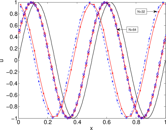
Refer to caption
Figure 6: A linear wave is propagated with constant velocity u¯^j=c¯jsubscript^¯𝑢𝑗subscript¯𝑐𝑗\hat{\underline{u}}_{j}=\underline{c}_{j} over 10 wavelengths. The coupled numerical schemes CN-RK3-CDM (dashed) and RK3-RK3-CDM (solid) with N=NRSS=NLES={32,64}𝑁subscript𝑁RSSsubscript𝑁LES3264N=N_{\rm RSS}=N_{{\rm LES}}=\{32,64\} are shown. The black line is the analytical result.

C.2 Coupled Advection Scheme: High Small Scale Resolution

Numerical convergence for the XLES coupled advection scheme is unconditionally obtained for increasing 3D resolution (NLESsubscript𝑁LESN_{\rm LES}\rightarrow\infty). This is valid for both coupled schemes: RK3-RK3-CDM and CN-RK3-CDM.

The convergence for the CN-RK3-CDM scheme with increasing small scale resolution (NRSSsubscript𝑁RSSN_{\rm RSS}\rightarrow\infty) and two choices of constant 3D resolution NLES={16,64}subscript𝑁LES1664N_{\rm LES}=\{16,64\} is additionally investigated. This kind of numerical convergence is not required to ensure a well defined and converging XLES approach.

A phase shift ΦΦ\Phi describes the numerical dispersion and thus measures the numerical accuracy (see figure 7).
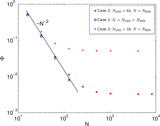
Refer to caption
Figure 7: ΦΦ\Phi is the phase difference between the analytical solution and the numerical result. Case 111: RK3-RK3-CDM scheme with N=NLES=NRSS𝑁subscript𝑁LESsubscript𝑁RSSN=N_{\rm LES}=N_{\rm RSS}. Case 222: CN-RK3-CDM scheme with N=NRSS𝑁subscript𝑁RSSN=N_{\rm RSS} and NLES={16,64}subscript𝑁LES1664N_{\rm LES}=\{16,64\}. For a CN-CDM scheme Tsai et al. (2002) analytically predict the behavior : ΦN2similar-toΦsuperscript𝑁2\Phi\sim N^{-2}.

We find the numerical accuracy of the coupled advection scheme increasing up to a resolution ratio NRSS/NLES10less-than-or-similar-tosubscript𝑁RSSsubscript𝑁LES10{N_{\rm RSS}/N_{\rm LES}}\lesssim 10. With higher ratios the numerical error of the coarse resolved scheme (RK3-CDM) dominates the coupled numerical error.

Thus the numerical accuracy is increased by increasing the resolved small scales within XLES up to some limit in addition to possibly resolving additional physical effects.

C.3 Coupled Advection Scheme: Spectral Scale Separation

In this section the CN-RK3-CDM scheme demonstrates the preservation of (spectrally separated) large and small scale properties which are represented w.l.o.g. in XLES-grid 222.

A multi-scale wave with the initial condition

u2,1subscript𝑢21\displaystyle{u}_{{2},1} =sin(4πx2,1)+0.2sin(128πx2,1)absent4𝜋subscript𝑥210.2128𝜋subscript𝑥21\displaystyle=\sin(4\pi x_{{2},1})+0.2\,\sin(128\pi x_{{2},1}) (54)
u3,1subscript𝑢31\displaystyle{u}_{{3},1} =[l31][l2]u2,1=sin(4πx3,1)absentdelimited-[]superscriptsubscript𝑙31delimited-[]subscript𝑙2subscript𝑢214𝜋subscript𝑥31\displaystyle=[l_{{3}}^{-1}][l_{2}]u_{{2},1}=\sin(4\pi x_{{3},1}) (55)

is propagated for 101010 wavelengths using NLES=64subscript𝑁LES64N_{\rm LES}=64 and NRSS=4096subscript𝑁RSS4096N_{\rm RSS}=4096 cells in the x2subscript𝑥2x_{2}-direction (advanced by Eq. (45) and (44)).

Note that the higher mode 0.2sin(128πx2,1)0.2128𝜋subscript𝑥210.2\,\sin(128\pi x_{{2},1}) is only resolved within XLES-grid 222 while XLES-grid 333 only captures the lower mode.

The box filtered and small scale properties are preserved, but little dispersed due to numerical effects (see figure 8).

Refer to caption
Figure 8: A multi-scale wave with the initial condition in Eq. (54) (lines) propagates for 101010 wavelengths. The full domain (small box) and one wave peak are shown. The big points corresponds to the 3D large scale field (NLES=64subscript𝑁LES64N_{\rm LES}=64 cells). The small points corresponds to the resolved small scales (NRSS=4096subscript𝑁RSS4096N_{\rm RSS}=4096). The black line corresponds to the analytical result.

References

  • Burbeau et al. (2001) Burbeau, A., Sagaut, P., Bruneau, C.-H., 2001. A problem-independent limiter for high-order runge-kutta discontinuous galerkin methods. J. Comput. Phys. 169, 111 – 150.
  • Cao and Echekki (2008) Cao, S., Echekki, T., 2008. A low-dimensional stochastic closure model for combustion large-eddy simulation. J. Turbul. 9, 1–35.
  • Cavaglieri and Bewley (2015) Cavaglieri, D., Bewley, T., 2015. Low-storage implicit/explicit Runge–Kutta schemes for the simulation of stiff high-dimensional ODE systems. J. Comput. Phys. 286, 172–193.
  • Crank and Nicolson (1996) Crank, J., Nicolson, P., 1996. A practical method for numerical evaluation of solutions of partial differential equations of the heat-conduction type. Adv. Comput. Math. 6, 207–226.
  • Ferziger and Peric (1999) Ferziger, J., Peric, M., 1999. Computational Methods for Fluid Dynamics. Springer.
  • Gadd (1978) Gadd, A. J., 1978. A split explicit integration scheme for numerical weather prediction. Quarterly Journal of the Royal Meteorological Society 104, 569–582.
  • Germano (1986) Germano, M., 1986. A proposal for a redefinition of the turbulent stresses in the filtered Navier-Stokes equations. Phys. Fluids 29, 2323–2324.
  • Germano et al. (1991) Germano, M., Piomelli, U., Moin, P., Cabot, W. H., 1991. A dynamic subgrid‐scale eddy viscosity model. Phys. Fluids A: Fluid Dynamics 3, 1760–1765.
  • Glawe et al. (2015) Glawe, C., Schmidt, H., Kerstein, A., Klein, R., 2015. XLES part II: From extended large eddy simulation to ODTLES. submitted to J. Comput. Phys.
  • Glawe et al. (2013) Glawe, C., Schulz, F., Gonzalez-Juez, E., Schmidt, H., Kerstein, A., 2013. ODTLES simulations of turbulent flows through heated channels and ducts. In: Proceedings of TSFP-8. Poitiers, France.
  • Gonzalez-Juez et al. (2011) Gonzalez-Juez, E. D., Schmidt, R. C., Kerstein, A. R., 2011. ODTLES simulation of wall-bounded turbulent flows. Phys. Fluids 23, 125102.
  • Kawamura (2014) Kawamura, H., Dec. 2014. DNS database. http://murasun.me.noda.tus.ac.jp/turbulence/index.html, [Online; accessed Dec 2014].
  • Kawamura et al. (1999) Kawamura, H., Abe, H., Matsuo, Y., 1999. DNS of turbulent heat transfer in channel flow with respect to Reynolds and Prandtl number effects. Int. J. Heat Fluid Fl. 20, 196–207.
  • Kerstein (1999) Kerstein, A. R., 1999. One-dimensional turbulence: Model formulation and application to homogeneous turbulence, shear flows, and buoyant stratified flows. J. Fluid Mech. 392, 277–334.
  • Kerstein et al. (2001) Kerstein, A. R., Ashurst, W. T., Wunsch, S., Nilsen, V., May 2001. One-dimensional turbulence: Vector formulation and application to free shear flows. J. Fluid Mech. 447, 85–109.
  • Lee and Moser (2014) Lee, M., Moser, R. D., 2014. Direct numerical simulation of turbulent channel flow up to Reτ=5200𝑅subscript𝑒𝜏5200Re_{\tau}=5200. under consideration for publication in J. Fluid Mech.
  • Leonard (1975) Leonard, A., 1975. Energy cascade in large-eddy simulations of turbulent fluid flows. Adv. Geophys. 18, 237–248.
  • LeVeque (1985) LeVeque, R. J., 1985. A large time step generalization of godunov’s method for systems of conservation laws. SIAM J. Numer. Anal. 22, 1051–1073.
  • Lignell et al. (2013) Lignell, D., Kerstein, A., Sun, G., Monson, E. I., 2013. Mesh adaption for efficient multiscale implementation of one-dimensional turbulence. Theor. Comput. Fluid Dyn. 27, 273–295.
  • McDermott (2005) McDermott, R. J., 2005. Toward one-dimensional turbulence subgrid closure for large-eddy simulation. Ph.D. thesis, University of Utah.
  • Meiselbach (2015) Meiselbach, F. T., 2015. Application of ODT to turbulent flow problems. Ph.D. thesis, BTU Cottbus-Senftenberg.
  • Menon and Kerstein (2011) Menon, S., Kerstein, A., 2011. The linear-eddy model. In: Echekki, T., Mastorakos, E. (Eds.), Turbulent Combustion Modeling: Advances, New Trends and Perspectives. Springer, pp. 221–247.
  • Pope (2000) Pope, S., 2000. Turbulent Flows. Cambridge University Press.
  • Sagaut (2006) Sagaut, P., 2006. Large Eddy Simulation for Incompressible Flows: An Introduction. Springer Verlag.
  • Sannan et al. (2013) Sannan, S., Weydahl, T., Kerstein, A. R., 2013. Stochastic simulation of scalar mixing capturing unsteadiness and small-scale structure based on mean-flow properties. Flow Turbul. Combust. 90, 189–216.
  • Schmidt et al. (2008) Schmidt, R. C., Kerstein, A. R., McDermott, R., 2008. ODTLES: A multi-scale model for 3D turbulent flow based on one-dimensional turbulence modeling. Comput. Methods Appl. Mech. Engrg. 199, 865–880.
  • Smits and Marusic (2013) Smits, A. J., Marusic, I., 2013. Wall-bounded turbulence. Phys. Today 66, 25–30.
  • Spalart and Allmaras (1992) Spalart, P., Allmaras, S., 1992. A one-equation turbulence model for aerodynamic flows. In: 30th Aerospace Sciences Meeting and Exhibit. American Institute of Aeronautics and Astronautics.
  • Spiteri and Ruuth (2002) Spiteri, R. J., Ruuth, S. J., 2002. A new class of optimal high-order strong-stability-preserving time discretization methods. SIAM J. Numer. Anal. 40, 469–491.
  • Tsai et al. (2002) Tsai, T., Yang, J., Huang, L., 2002. Hybrid finite-difference scheme for solving the dispersion equation. J. Hydraul. Eng. 128, 78–86.
  • Zha and Lingamgunta (2003) Zha, G., Lingamgunta, C., 2003. On the accuracy of runge-kutta methods for unsteady linear wave equation. In: 41st Aerospace Sciences Meeting and Exhibit. American Institute of Aeronautics and Astronautics.