Aging Wiener-Khinchin Theorem

Abstract

The Wiener-Khinchin theorem shows how the power spectrum of a stationary random signal $I(t)$ is related to its correlation function $\left\langle I(t)I(t+\tau)\right\rangle$. We consider non-stationary processes with the widely observed aging correlation function $\langle I(t)I(t+\tau)\rangle\sim t^{\gamma}\phi_{\rm EN}(\tau/t)$ and relate it to the sample spectrum. We formulate two aging Wiener-Khinchin theorems relating the power spectrum to the time and ensemble averaged correlation functions, discussing briefly the advantages of each. When the scaling function $\phi_{\rm EN}(x)$ exhibits a non-analytical behavior in the vicinity of its small argument we obtain aging $1/f$ type of spectrum. We demonstrate our results with three examples: blinking quantum dots, single file diffusion and Brownian motion in a logarithmic potential, showing that our approach is valid for a wide range of physical mechanisms.

Understanding how the strength of a signal is distributed in the frequency domain, is central both in practical engineering problems and in Physics. In many applications a random process $I(t)$ recorded in a time interval $(0,t_{m})$ is analyzed with the sample spectrum $S_{t_{m}}(\omega)=|\int_{0}^{t_{m}}I(t)\exp(-i\omega t){\rm d}t|^{2}/t_{m}$, which is investigated in the limit of a long measurement time $t_{m}$. For stationary processes, the fundamental Wiener-Khinchin theorem Kubo relates between the power spectrum density and the correlation function $C(\tau)=\langle I(t)I(t+\tau)\rangle$

$$\lim_{t_{m}\to\infty}\langle S_{t_{m}}(\omega)\rangle=2\int_{0}^{\infty}C(\tau)\cos(\omega\tau){\rm d}\tau.$$ (1)

However in recent years there is growing interest in the spectral properties of non-stationary processes, where the theorem is not valid Bouchaud ; Margolin06 ; Eliazar ; Aquino ; Niemann ; Rod ; Bouchaud96 ; Silv ; Schriefl . In general, there seems no point to discuss and classify spectral properties of all possible non-stationary processes. Luckily, a wide class of Physical systems and models exhibit a special type of correlation functions $\langle I(t)I(t+\tau)\rangle\sim t^{\gamma}\phi_{{\rm EN}}(\tau/t)$ for an observable $I(t)$ and the subscript ${\rm EN}$ denotes an ensemble average. Such correlation functions, describing what is referred to as physical aging, appear in a vast array of systems and models ranging from glassy dynamics Bouchaud ; Barrat ; Dean ; Bertin , blinking quantum dots Margolin04 , laser cooled atoms DechantPRX13 , motion of a tracer particle in a crowded environment Lizana ; Leibovich , elastic models of fluctuating interfaces Taloni , deterministic noisy Kuramoto models Ionita , granular gases Bordova , and deterministic intermittency AgingELI , to name only a few examples. In some cases the scaling function exhibits a second scaling exponent, $\langle I(t)I(t+\tau)\rangle\sim t^{\gamma}\phi_{{\rm EN}}(\tau/t^{\beta})$, or even a logarithmic time dependence Bertin , however here we will avoid this zoo of exponents, and attain classification of the spectrum for the case $\beta=1$.

A natural problem is to relate between the sample spectrum of such processes and the underlying correlation function Margolin06 . That such a relation actually exists is obvious from the basic definition of the sample spectrum, see Eq. (2) below. However, here we find a few interesting insights. First, the correlation function in its scaling form $\langle I(t)I(t+\tau)\rangle\sim t^{\gamma}\phi_{{\rm EN}}(\tau/t)$ is valid in Physical situations, in the limit of large $t$ and $\tau$. We here first formulate a theorem for ideal processes, where the aging correlation function is valid for all $\tau$ and $t$, and then in the second part of the Letter, explore by comparison to realistic models the domain of validity of the ideal models. As a rule of thumb the aging Wiener-Khinchin theorem presented here for ideal models works well in the limit of low frequency. Further the limit of small frequency and measurement time $t_{m}$ being large is not interchangeable and should be taken with care. Secondly, the spectrum in these processes depends on time $t_{m}$, as already observed in Margolin06 ; Sadegh . The non-stationarity also implies a third theme, namely that the ensemble average correlation function is non identical to the time averaged correlation function, in contrast with the usual Wiener-Khinchin scenario. Thus we formulate two theorems, relating between time and ensemble average correlation functions and the sample spectrum. The choice of theorem to be used in practice depends on the application.

In physics the power spectrum is not only a measure of the strength of frequency modes in a system. Nyquist’s fluctuation dissipation theorem, for systems close to thermal equilibrium and hence stationary, states that the ratio between the power spectrum and the imaginary part of the response function, $\chi(\omega)$, is given by temperature, i.e. $k_{B}T=\pi\omega S(\omega)/2\Im\left[\chi(\omega)\right]$ FDT.Kubo . Similarly, effective temperatures are routinely defined by relating measurements of power spectrum and response functions of non-stationary processes LFC ; Bellon ; Crisanti . Our goal here is to provide the connection between the sample spectrum and the correlation functions, without which the meaning of the effective temperature becomes some what ambiguous. More practically, an experimentalist who uses the sample spectrum to estimate the spectrum of a non-stationary process, might wish to extract from it the time and/or the ensemble averaged correlation functions, and for that our work is valuable.

Aging Wiener-Khinchin theorem for time averaged correlation functions. For a general process, the autocorrelation function $\langle I(t)I(t+\tau)\rangle$ is a function of its two variables, unlike stationary processes, where the correlation function depends only on the time difference $\tau$. Using the definition of the sample spectrum we have

$$t_{m}\langle S_{t_{m}}(\omega)\rangle=\int_{0}^{t_{m}}{\rm d}t_{1}\int_{0}^{t_{m}}{\rm d}t_{2}e^{i\omega(t_{2}-t_{1})}\langle I(t_{1})I(t_{2})\rangle.$$ (2)

We identify in this equation the ensemble average correlation function, but a formalism based on a time average will turn out more connected to the original Wiener-Khinchin theorem, as we proceed to show. A change of variable $\tau=t_{2}-t_{1}$ and relabeling integration variables gives

$$\langle S_{t_{m}}(\omega)\rangle={2\over t_{m}}\int_{0}^{t_{m}}{\rm d}\tau(t_{m}-\tau)\langle C_{{\rm TA}}(t_{m},\tau)\rangle\cos\left(\omega\tau\right).$$ (3)

Here the time averaged correlation function is defined as

$$C_{{\rm TA}}\left(t_{m},\tau\right)={1\over t_{m}-\tau}\int_{0}^{t_{m}-\tau}{\rm d}t_{1}I(t_{1})I(t_{1}+\tau).$$ (4)

We now insert in Eq. (3) an aging correlation function

$$\langle C_{{\rm TA}}(t_{m},\tau)\rangle=(t_{m})^{\gamma}\varphi_{{\rm TA}}\left(\tau/t_{m}\right),$$ (5)

defining a new integration variable $0<\tilde{\tau}=\tau/t_{m}<1$ we find

$$\langle S_{t_{m}}(\omega)\rangle=2(t_{m})^{1+\gamma}\int_{0}^{1}{\rm d}\tilde{\tau}\left(1-\tilde{\tau}\right)\varphi_{{\rm TA}}\left(\tilde{\tau}\right)\cos\left(\omega t_{m}\tilde{\tau}\right).$$ (6)

This formula relates between the time average correlation function and the average of the sample spectrum, for ideal processes in the sense that we have assumed that the scaling of the correlation function holds for all times. It shows that the frequency $\omega$ times $t_{m}$ is the scaling variable of the power spectrum.

Aging Wiener-Khinchin formula for the ensemble averaged correlation function. We now relate the power spectrum with the ensemble averaged correlation function which has a scaling form

$$\langle I(t+\tau)I(t)\rangle=t^{\gamma}\phi_{{\rm EN}}(\tau/t).$$ (7)

The two correlation functions are related with Eq. (4), which upon averaging gives

$$\varphi_{{\rm TA}}(x)=x^{\gamma}y(x)\int_{y(x)}^{\infty}{\phi_{{\rm EA}}(z)\over z^{2+\gamma}}{\rm d}z$$ (8)

with $y(x)=x/(1-x)$. Considering the case $\gamma=0$ we insert Eq. (8) in Eq. (6) and find

$$\left\langle S_{t_{m}}(\omega)\right\rangle=2t_{m}\int_{0}^{1}\phi_{{\rm EA}}\left(\frac{x}{1-x}\right){\tilde{\omega}x\sin(\tilde{\omega}x)+\cos(\tilde{\omega}x)-1\over\left(\tilde{\omega}x\right)^{2}}{\rm d}x$$ (9)

with $\tilde{\omega}=\omega t_{m}$. For the more general case $\gamma\neq 0$ we show in the supplementary material that

$$\left\langle S_{t_{m}}(\omega)\right\rangle=\frac{2(t_{m})^{\gamma+1}}{2+\gamma}\int_{0}^{1}(1-x)^{\gamma}\phi_{{\rm EN}}\left(\frac{x}{1-x}\right){{}_{1}F_{2}}\left(1+\frac{\gamma}{2};\frac{1}{2},2+\frac{\gamma}{2};-\left(\frac{\tilde{\omega}x}{2}\right)^{2}\right){\rm d}x,$$ (10)

where ${}_{1}F_{2}$ is a hypergeometric function and $\gamma>-2$.

This relation between the ensemble average correlation function and the sample averaged spectrum is useful for theoretical investigations, when a microscopical theory provides the ensemble average. Alternatively one may use the relation Eq. (8) to compute the time average correlation function from the ensemble average (if the latter is known) and then use the time averaged formalism Eq. (6) which is based on a simple cosine transform. The transformation Eq. (10) depends on $\gamma$, which in experimental situation might be unknown (though it could be estimated from data), while Eq. (6) does not, still both formalisms are clearly identical and useful.

Relation with $1/f$ noise. We now consider a class of aging correlation functions, with the additional characteristic behavior for small variable $\tau/t$

$$\langle I(t)I(t+\tau)\rangle\sim t^{\gamma}\left[A_{{\rm EN}}-B_{{\rm EN}}\left({\tau\over t}\right)^{\nu}\right].$$ (11)

Here $A_{{\rm EN}},B_{{\rm EN}}>0,0<\nu<1,\gamma>-1$ and $\gamma-\nu>-1$. Physical examples will soon follow. We use Eqs. (4,5,7,8) and by comparison of coefficients of small argument expansion, we show that the time averaged correlation function has a similar expansion, with $\langle C_{{\rm TA}}(t,\tau)\rangle\sim t^{\gamma}\left[A_{{\rm TA}}-B_{{\rm TA}}(\tau/t)^{\nu}+\cdots\right]$ with $A_{{\rm TA}}=A_{{\rm EA}}/(1+\gamma)$ and $B_{{\rm TA}}=B_{{\rm EA}}/(1-\nu+\gamma)$. We can then insert this expansion in Eq. (6), by integration by parts and using $\omega t_{m}=2\pi n\gg 1$ where $n$ is an integer

$$\langle S_{t_{m}}(\omega)\rangle\sim{2\Gamma(1+\nu)\sin\left({\pi\nu\over 2}\right)B_{{\rm EA}}\over\left(\gamma-\nu+1\right)(t_{m})^{\nu-\gamma}\omega^{1+\nu}}.$$ (12)

We see that the non-analytical expansion of the correlation function, in small argument, leads to a $1/f$ type of noise, with an amplitude that depends on measurement time. Such an aging effect in the power spectrum was recently measured for blinking quantum dots Sadegh , so this shall be our first example.

Blinking quantum dots and trap model. As measurements show, blinking quantum dots, nano-wires and organic molecules exhibit episodes of fluorescence intermittency, switching randomly between on and off states Kuno ; Kraft ; PhysTodayBarkai . The on and off waiting times are random with a common power law waiting time distribution $\psi(\tau)\sim A\tau^{-(1+\alpha)}$, a behavior valid under certain conditions, like low temperature and weak external laser field. For this simple renewal model, and when the average on and off times diverge, namely $0<\alpha<1$, we have $\gamma=0$ and the correlation function, with intensity in the on state taken to be $I_{0}$ and in the off state to be zero, is Margolin04

$$\phi_{{\rm EN}}(x)=I_{0}^{2}\left[{1\over 2}-\frac{\sin(\pi\alpha)}{4\pi}B\left({x\over 1+x};1-\alpha,\alpha\right)\right]$$ (13)

where $x=\tau/t$ and $B(z;a,b)$ is the incomplete beta function. Importantly, this type of correlation function describes not only blinking dots, but also the trap model, a well known model of glassy dynamics Dean . The connection between the two systems are the power law waiting times in micro-states of the system, though for the trap model $\alpha=T/T_{g}$ where $T$ is temperature, while $0.5<\alpha<0.8$ in quantum dots experiments. Eq. (13) is valid only in a scaling limit for large $\tau$ and $t$ when the microscopic details of the model, e.g. the shape of the waiting time distribution $\psi(\tau)$ for short on and off blinking events, are irrelevant. Thus the scaling solution is controlled only by the parameter $\alpha$. The time averaged correlation function is obtained from Eqs. (8,13)

$$\phi_{{\rm TA}}(x)={I_{0}^{2}\over 4}+$$ (14)

$${I_{0}^{2}\over 4}\frac{\sin(\pi\alpha)}{\pi}\left[{B\left(1-x,\alpha,1-\alpha\right)\over 1-x}-{1\over\alpha}\left({x\over 1-x}\right)^{1-\alpha}\right],$$

which is clearly non-identical to the corresponding ensemble averaged one. We may now use either Eq. (6) for the time average or Eq. (9) for the ensemble average to obtain $S_{t_{m}}(\omega)$. Since $\gamma=0$ we use Eq. (9) and find

$$\langle S_{t_{m}}(\omega)\rangle/t_{m}=I_{0}^{2}\left\{\frac{{\rm sinc}^{2}\left(\frac{\tilde{\omega}}{2}\right)}{4}+\frac{1}{2\tilde{\omega}}\Im\left[{M}(1-\alpha,2;\imath\tilde{\omega})\right]\right\},$$ (15)

where $M(a,b;z)$ is the Kummer confluent hypergeometric function and $\Im\left[.\right]$ refers to its imaginary part. We note that the ${\rm sinc^{2}(\tilde{\omega}/2})$ term is the spectrum contribution from a constant $\left\langle\bar{I}^{2}\right\rangle$. As shown in Fig. 1 the spectrum Eq. (15) perfectly matches finite time simulation of the process where we used $\psi(\tau)=\alpha\tau^{-(1+\alpha)}$ for $\tau>1$, $\alpha=0.5$, $I_{0}=1$ and an average over $10^{3}$ on-off blinking processes was made. This indicates that the scaling approach works well, even for reasonable finite measurement time. The theory predicts nicely not only the generic $1/f$ behavior but also the fine oscillations and the crossover to the low frequency limit. As Fig. 1 demonstrates when $\omega t_{m}$ is large, we get the $1/f$ noise result, which according to Eq. (12) is

$$\langle S_{t_{m}}(\omega)\rangle\sim{I_{0}^{2}\cos\alpha\pi/2\over 2\Gamma(1+\alpha)}(t_{m})^{\alpha-1}\omega^{\alpha-2}.$$ (16)

for $0<\alpha<1$. In this model $\nu=1-\alpha$ as the small argument expansion of Eq. (13) shows. The asymptotic Eq. (16) agrees with previous approaches Margolin06 , the latter missing the low frequency part of the spectrum, and the fine structure of the spectrum presented in Fig. 1, since for those non trivial aspects of the theory one needs the aging Wiener-Khinchin approach developed here. Finally, we have assumed that the start of the blinking process at $t=0$ (corresponding to the switching on of the laser field) is the moment in time where we start recording the power spectrum. If one waits a time $t_{w}$ before start of the measurement, the power spectrum will depend on the waiting time $t_{w}$ since the process is non-stationary Bouchaud .

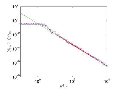
Figure 1: (color online). Power spectral density for the blinking quantum dot model with $\alpha=0.5$ with measurement time $t_{m}=10^{5}$. Theory Eq. (15) (red line) perfectly matches finite time simulation (blue $\circ$) and asymptotically the $1/f$ noise Eq. (16) (green line).

We note that a model with cutoffs on the aging behaviors was investigated in Godec , in this case the asymptotic behavior is normal, namely the Wiener-Khinchin theorem holds. Indeed in experiments on blinking quantum dots with a measurement time of $1800$ seconds the aging of the spectrum is still clearly visible Sadegh , the latter measurement time is long in the sense that blinking events are observed already on the $\mu$ Sec. time scale. Hence cutoffs, while possibly important in some applications, are not relevant at least in this experiment.

Single file diffusion. We consider a tagged Brownian particle in an infinite unidimensional system, interacting with other identical particles through hard core collisions Harris ; Krapivsky ; Hegde . This well known model of a particle in a crowded pore, is defined through the free diffusion coefficient $D$ describing the motion of particles between collision events and the averaged distance between particles $a$. Initially at time $t=0$ the particles are uniformly distributed in space and the tagged particle is on the origin. In this many body problem, the motion of the tracer is sub-diffusive $\langle x^{2}(t)\rangle\sim a\sqrt{D/\pi}\sqrt{t}$ since the other particles are slowing down the tracer particles via collisions Harris . Normal diffusion is found only at very short times $t<a^{2}/D$ when the tracer particle has not yet collided with the other surrounding Brownian particles. Our observable (so far called $I(t)$) is the position of the tracer particle in space $x(t)$. The correlation function in the long time scaling limit is Leibovich ; Lizana

$$\langle x(t)x(t+\tau)\rangle=a\sqrt{{D\over\pi}}\sqrt{t}\left(\sqrt{1+{\tau\over t}}+1-\sqrt{\tau\over t}\right).$$ (17)

Such a correlation function describes also the coordinate of the Rouse chain model, a simple though popular model of Polymer dynamics Rouse . Then by insertion and integration we find using Eqs. (6,8)

$$(t_{m})^{-3/2}\sqrt{\frac{\pi}{Da^{2}}}\left\langle S_{t_{m}}(\omega)\right\rangle =\frac{1}{\tilde{\omega}^{5/2}}\sqrt{\tilde{\omega}}(2+\cos(\tilde{\omega}))$$

$$-\frac{\sqrt{2\pi}}{2\tilde{\omega}^{5/2}}(1+2\cos(\tilde{\omega})){\cal{C}}(\sqrt{2\tilde{\omega}/\pi})$$

$$+\frac{\sqrt{2\pi}}{\tilde{\omega}^{5/2}}{\cal{S}}(\sqrt{2\tilde{\omega}/\pi})(-\tilde{\omega}+\sin(\tilde{\omega})),$$

where the Fresnel functions are defined as ${\cal{C}}(u)\equiv\int_{0}^{u}\cos(\pi t^{2}/2)dt$ and ${\cal{S}}(u)\equiv\int_{0}^{u}\sin(\pi t^{2}/2)dt$. Generating $10^{3}$ trajectories of single file motion, for a system with $2001$ particles, with the algorithm in Leibovich we have found the sample spectrum of the process $x(t)$. As Fig. 2 demonstrates theory and simulation for $\langle S_{t_{m}}(\omega)\rangle$ perfectly match without fitting. From the correlation function Eq. (17) we have $\gamma=\nu=1/2$ and hence according to Eq. (12)

$$\langle S(\omega)\rangle\sim\sqrt{{a^{2}D\over 2}}\omega^{-3/2}$$ (19)

for $\omega t_{m}\gg 1$. This equation is the solid line presented in Fig. 2 which is seen to match the exact theory already for not too large values of $\omega t_{m}$. As in the previous example aging Wiener-Khinchin framework is useful in the predictions of the deviations from the asymptotic result; as Fig. 2 clearly demonstrates some non-trivial wiggliness perfectly matching simulations.

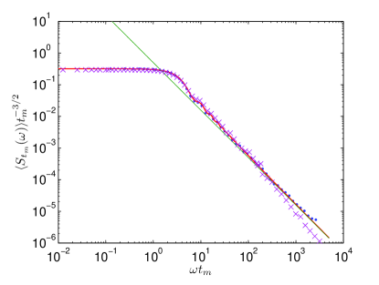
Figure 2: (color online). The power spectrum of tagged particle motion $x(t)$ with measurement times $t_{m}=10^{3}$ (blue $\bullet$) and $t_{m}=10^{2}$ (pink $\times$). For this single file model theory Eq. (Aging Wiener-Khinchin Theorem) (red line) and asymptotic $1/f$ approximation Eq. (19) nicely match simulation results. In simulation we used $D=1/2$ and $a=1$. Finite time deviations for $t_{m}=10^{2}$ are observed at high frequency as discussed in text.

As mentioned in the introduction we have assumed a scaling form of the correlation function Eqs. (5,7), which works in the limit of $t,\tau\rightarrow\infty$. Information on the correlation function for short times is needed to estimate the very high frequency limit of the spectrum. Hence the deviations at high frequencies in Fig. 2 are expected. As measurement time is increased the spectrum plotted as a function of $\omega t_{m}$ perfectly approaches the predictions of our theory (see also the following example and Fig. 3).

Diffusion in a logarithmic potential. While our previous examples are based on long tailed trapping times and many body interactions which lead to a long term memory in the dynamics we will now briefly discuss a third mechanism using over damped Langevin dynamics in a system which attains thermal equilibrium. Consider the position $x(t)$, which is the observable $I(t)$, of a particle with mass $m$ in a logarithmic potential $U(x)=U_{0}\ln(1+x^{2})/2$

$${{\rm d}x\over{\rm d}t}=-{1\over m\bar{\gamma}}{\partial U\over\partial x}+\eta(t).$$ (20)

Here the noise is white with mean equal zero satisfying the fluctuation dissipation theorem and $\bar{\gamma}$ is a friction constant. Under such conditions the equilibrium probability density function is given by Boltzmann’s law $P_{{\rm eq}}(x)=\exp[-U(x)/k_{b}T]/Z$, where $Z$ is the partition function and $T$ is the temperature. A key observation is that the potential is asymptotically weak in such a way that $P_{{\rm eq}}\sim x^{-U_{0}/k_{b}T}$ for large $x$ and for normalization to be finite we assume $U_{0}/k_{b}T>1$. The system thus exhibits large fluctuations in its amplitude in the sense that in equilibrium $\langle x^{2}\rangle$ diverges in the regime $U_{0}/k_{b}T<3$. Of course for any finite measurement time the variance of $x(t)$, starting on the origin, is increasing with time but finite. Let $\alpha=U_{0}/(2k_{b}T)+(1/2)$ and we focus on the case $1<\alpha<2$. The correlation function in this case was investigated in Dechant2012 . We here study only the $1/f$ part of the spectrum, demonstrating the versatility of the theory using equation (12), since unlike previous cases the correlation function is cumbersome. To find the $1/f$ noise we need to know, from the ensemble average correlation function, $\gamma,\nu$ and $B_{{\rm EN}}$, while $A_{{\rm EN}}$ must be finite (similar steps for other models will be published elsewhere Notation ). As detailed in the SM SM $\gamma=\nu=2-\alpha$ and $B_{\rm EN}=\sqrt{\pi}(4D)^{2-\alpha}c_{1}/\left[Z\Gamma(\alpha)\Gamma(1+\alpha)\right]$ and $A_{\rm EN}=B_{\rm EN}\Gamma(1+\alpha)/\left[\sqrt{\pi}(2-\alpha)c_{1}\right]$ with $D=k_{b}T/m\bar{\gamma}$ the diffusion constant according to the Einstein relation, hence by using Eq. (12) we obtain

$$\left\langle S(\omega)\right\rangle\sim 2\Gamma(3-\alpha)\sin\left({\alpha\pi\over 2}\right)B_{{\rm EN}}{1\over\omega^{3-\alpha}}.$$ (21)

The constant $c_{1}$ is given in terms of an integral of a special function SM . We have simulated the Langevin equation (20) and obtained finite time estimates for the power spectrum, which match the prediction Eq. (21) as shown in Fig. 3 without fitting. Importantly, the model of diffusion in logarithmic field is applicable in many systems, including diffusion of cold atoms in optical lattices Marksteiner .

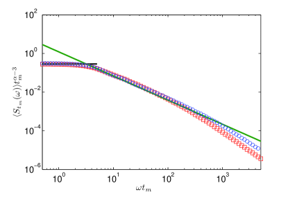
Figure 3: (color online). Power spectrum of Brownian motion in a logarithmic potential (symbols) matches the asymptotic theory predicting $1/f$ type of noise Eq. (21) (green line). We use $\alpha=1.75,t_{m}=5\cdot 10^{2}$ (red $\triangle$) and $t_{m}=2\cdot 10^{3}$ (blue $\circ$) with $U_{0}=1$, $\bar{\gamma}=1$ and $m=1$. In addition we plot the theoretical zero frequency prediction $\langle S_{t_{m}}(0)\rangle$ (black line), see SM. The ensemble average was taken over $5000$ realizations.

Summary and Discussion. We have presented general relations between the sample spectrum and the time/ensemble averaged correlation function Eqs. (3,9), respectively. Those relations work for Physical models in the limit $t_{m}\rightarrow\infty$ and $\omega\rightarrow 0$ while the product $\omega t_{m}$ is finite. In experiment $t_{m}$ might be long, but it is always finite. Hence, the theorem will work in practice in the low frequency regime. Indeed, a close look at Fig. 2, 3 shows finite time deviation at large frequencies, the aging spectrum is approached when $t_{m}$ is increased. The fact that the scaled correlation function is observed in a great variety of different systems, serves as evidence of the universality of our main results, i.e. Eqs. (3,9).

- (1) R.Kubo, M.Toda, and H. Hashitsume, Statistical Physics II- Nonequilibrium Statistical Mechanics, Springer (1995).
- (2) J. P. Bouchaud, L. F. Cugliandolo, J. Kurchan, and M. Mzard, in Spin Glasses and Random Fields, edited by A.P. Young (World Scientific, Singapore, 1998). (also in cond-mat/9702070)
- (3) G. Margolin, and E. Barkai, J. Stat. Phys. 122, 137 (2006).
- (4) I. Eliazar, and J. Klafter, Phys. Rev. Lett. 103, 040602 (2009).
- (5) G. Aquino, M. Bologna, P. Grigoli, and B. J. West, Phys. Rev. Lett. 105 040601 (2010).
- (6) M. Niemann, H. Kantz, and E. Barkai, Phys. Rev. Lett, 110, 140603 (2013).
- (7) M. A. Rodriguez, Phys. Rev. E. 90 042122 (2014).
- (8) C. Monthus, and J-P. Bouchaud, J. Phys. A: Math. Gen. 29, 3847-3869 (1996).
- (9) L. Silvestri, L. Fronzoni, P. Grigolini, and P. Allegrini, Phys. Rev, Lett. 102, 014502 (2009).
- (10) J. Schriefl, M. Clusel, D. Carpentier, and P. Degiovanni, Phys. Rev. B 72, 035328 (2005).
- (11) E. Bertin, and J. P. Bouchaud, J. of Physics A: mathematical and general 35 3039 (2002).
- (12) A. Barrat, R. Burioni, and M. Mezard, J. Phys. A. Math. Gen. 29, 1311 (1996).
- (13) J. P. Bouchuad, and D. S. Dean J. Phys. I France 5 265 (1995).
- (14) G. Margolin, and E. Barkai, J. Chem. Phys. 121, 1566 (2004).
- (15) A. Dechant, E. Lutz, D. A. Kessler, and E. Barkai, Phys. Rev. X 4, 011022 (2014).
- (16) L. Lizana, M. A. Lomholt, and T. Ambjrnsson, Physica A, 395 148 153 (2014).
- (17) N. Leibovich, and E. Barkai, Phys. Rev. E 88, 032107, (2013).
- (18) A. Taloni, A. Chechkin, and J. Klafter Phys. Rev. Lett. 104, 160602 (2010).
- (19) F. Ionita, and H. Meyer-Ortmanns, Phys. Rev. Lett. 112, 094101 (2014).
- (20) A. Bordova, A. V. Chechkin, A. G. Cherstvy, and R. Metzler, arXiv:1501.04173 [cond-mat.stat-mech] (2015)
- (21) E. Barkai, Phys. Rev. Lett. 90, 104101 (2003).
- (22) S. Sadegh, E. Barkai, and D. Krapf, New. J. of Physics 16 113054 (2014).
- (23) R. Kubo, Rep. Prog. Phys. 29, 255 (1966).
- (24) L. Bellon and S. Ciliberto, Physica D 168, 325 (2002).
- (25) L. F. Cugliandolo, J. Kurchan, and G. Parisi, cond-mat/9406053 (1994). L. F. Cugliandolo, J. Kurchan, and L. Peliti, Phys. Rev. E 55, 3898 (1997).
- (26) A. Crisanti, and F. Ritort, J. Phys. A: Math. Gen. 36, R181-R290 (2003).
- (27) P. Frantsuzov, M. Kuno, B. Janko and R. A. Marcus, Nature Phys. 4, 519 (2008).
- (28) F. D. Stefani, J. P. Hoogenboom, and E. Barkai, Phys. Today 62(2), 34 (2009).
- (29) D. Krapf, Phys. Chem. Chem. Phys., 15, 459 (2013).
- (30) A. Godec, and R. Metzler, Phys. Rev. E. 88, 012116 (2013).
- (31) T. E. Harris, J.Appl.Probab. 2 323 (1965).
- (32) P. L. Krapivsky, K. Mallick, and T. Sadhu, Phys. Rev. Lett. 113, 078101 (2014).
- (33) C. Hegde, S. Sabhapandit, and A. Dhar, Phys. Rev. Lett. 113, 120601 (2014).
- (34) P. E. Rouse, J. Chem. Phys. 21 1272 (1953).
- (35) A. Dechant, E. Lutz, D. A. Kessler, and E. Barkai Phys. Rev. E 85, 051124 (2012).
- (36) N. Leibovich, and E. Barkai, in preparation.
- (37) See Supplemental Material
- (38) S. Marksteiner, K. Ellinger, and P. Zoller, Phys. Rev. A, 53, 3409 (1996).