Gravitational waves induced by spinor fields

Abstract

In realistic model-building, spinor fields with various masses are present. During inflation, spinor field may induce gravitational waves as a second order effect. In this paper, we calculate the contribution of single massive spinor field to the power spectrum of primordial gravitational wave by using retarded Green propagator. We find that the correction is scale-invariant and of order $H^{4}/M_{P}^{4}$ for arbitrary spinor mass $m_{\psi}$. Additionally, we also observe that when $m_{\psi}\gtrsim H$, the dependence of correction on $m_{\psi}/H$ is nontrivial.

I Introduction

General relativity strongly suggests the existence of gravitational waves. Through the study of gravitational waves, we might get rich information about new physics in the very early universe directly since there may be footprints left in it if the corresponding processes happened energetically. Recently, besides B-mode polarization of CMB [1],[2], gravitational waves searching are proposed or underway on smaller scale by interferometers like VIRGO, DECIGO and LISA, which make the studies relevant with gravitational waves acquire increasing attentions.

The primordial gravitational wave may be produced from quantum fluctuations of vacuum during inflation [3],[4],[5], which is scale-invariant and is regarded as a smoking gun for inflation. The primordial gravitational waves may record some physical information during inflation, which can hardly be encoded by scalar perturbation, e.g. a step-like variation of primordial gravitational waves speed will result in the oscillating tensor spectrum [6]. Thus, every possible way of affecting gravitational waves spectrum is significant and worth studying. There are also other mechanisms producing gravitational waves in the early universe, e.g. cosmic defeats [7, 8], bubble collisions [9, 10].

Back in the very early stage of universe, there must be numerous fields besides the inflaton field. In linear order, the scalar fields other than inflaton can only generate isocurvature perturbations, see [11],[12] for the effect of massive isocurvaton on the density perturbations, see also [13],[14],[15]. When the action is expanded to third order in perturbations, one may see that the scalar fields can source gravity at quadratic order. This motivates the mechanism of inducing gravitational waves by introducing a spectator scalar field [16], see also [17],[18].

Spinor fields with various masses should also be present in early universe, as a consequence of realistic model-building. During inflation, these spinor fields look like spectators, i.e. they do not affect the inflationary dynamics at neither the background nor the linear order fluctuations level. Thus, similar to scalar spectators, they may also source gravity at quadratic order. In addition, there are also some studies about gravitational waves sourced by production of particles see e.g.[19],[20], by production of fermion see [21, 22].

There are mainly two kinds of methods of calculating the corrections to the power spectrum. One is loop correction with in-in formalism [23]. The loop correction of a Dirac field to the scalar power spectrum was studied comprehensively in [24]. In Ref.[25], we have calculated the loop correction of Dirac field to the gravitational wave power spectrum. The other is inducing gravitational waves as a second order effect, using retarded Green propagator, and regarding the spectator fields as sources.

In this paper, we will calculate the contribution of massive spinor field during inflation to the gravitational wave power spectrum by using retarded Green propagator. We find that the correction is scale-invariant and of order $H^{4}/M_{P}^{4}$ for arbitrary mass $m_{\psi}$. When $m_{\psi}\gtrsim H$, the dependence of correction on $m_{\psi}/H$ is nontrivial. In Section II we give a brief introduction to the background dynamics of spinor field in inflationary cosmology. In Section III, we calculate the primordial gravitational wave spectrum induced by spinor field and give our result. The conclusion is given in Section IV. In Appendix A, we show the calculation process of spin sum for massive fermions, which is necessary for our computation of the massive spinor field’s contribution to the two point correlation function of tensor.

II Dynamics of Dirac field

In Ref.[25], we have described in detail the dynamics of a spinor field which is minimally coupled to Einstein gravity, see also Refs. [26, 27] for detailed introduction and [28] for the cosmology with spinor fields. In this section, we will briefly review it.

Taking into account the spatial dependence of the Dirac field, the equations of motion for it is given by

$$i\gamma^{0}(\dot{\psi}+\frac{3}{2}H\psi)-i\gamma^{i}\frac{\partial_{i}}{a}\psi-m_{\psi}\psi = 0~{},$$ (1)

where $H$ is the Hubble parameter during inflation. As usual, the Fourier transformation of $\psi(\mathbf{x},t)$ is

$$\psi(\mathbf{x},t)=\int\mathrm{d}^{3}p~{}e^{i\mathbf{p}\cdot\mathbf{x}}\sum_{s}\left[\alpha_{\mathbf{p},s}X_{\mathbf{p},s}(t)+\beta^{\dagger}_{-\mathbf{p},s}W_{-\mathbf{p},s}(t)\right]~{},$$ (2)

where $s=\pm{1}/{2}$ is the spin of the Dirac field, and also the annihilation operators of the Dirac field satisfies the anti-commutative relation.

The Fourier modes $X_{\mathbf{p},s}(t)$, $W_{\mathbf{p},s}(t)$ satisfy the equations of motion shown in Eq.(1). Solving the equation of motion in comoving time coordinate $\tau\equiv\int dt/a$, we obtain

$$X_{k,\pm}(\tau) = \frac{i\sqrt{-\pi k\tau}}{2(2\pi a)^{3/2}}e^{\pm{\pi r}}H^{(1)}_{{1}/{2}\mp ir}(-k\tau)~{},$$ (3)

where $H^{(1)}$ is the first kind of the Hankel function and $r=m_{\psi}/H$, and also we have made use of Bunch-Davies vacuum as initial condition to determine the coefficient of the Hankel function.

III Induced Gravitational Wave

In Einstein gravity, the quadratic action of tensor perturbation and the interaction between it and the Dirac field are

$$S^{(2)}=\int d^{4}x{aM_{P}^{2}\over 8}\left(h_{ij}^{\prime 2}-(\partial h_{ij})^{2}\right),$$ (4)

$${S}_{\psi{\bar{\psi}}h}^{(3)} = \int d^{4}x{a^{2}\over 2}T^{ij}h_{ij}$$ (5)

$$= i\int d^{4}x~{}\frac{a^{2}}{8}\left(\bar{\psi}\gamma^{i}(\partial^{j}\psi)+\bar{\psi}\gamma^{j}(\partial^{i}\psi)-(\partial^{i}\bar{\psi})\gamma^{j}\psi-(\partial^{j}\bar{\psi})\gamma^{i}\psi\right)h_{ij},$$

respectively. Then the equation of motion for $h_{ij}$, sourced by Dirac field at second-order, can be expressed in conformal time as

$$h^{\prime\prime}_{ij}+2\frac{a^{\prime}}{a}h^{\prime}_{ij}-\partial^{2}h_{ij}=\frac{2a}{M_{P}^{2}}T_{ij}^{TT},$$ (6)

where $T_{ij}^{TT}=\Pi_{ij}^{~{}~{}lm}T_{lm}$, and $T_{ij}$ is defined in Eq.(5), and the TT-projection tensor $\Pi_{ij}^{~{}~{}lm}\equiv P_{i}^{m}P_{j}^{l}-\frac{1}{2}P_{ij}P^{lm}$, while $P_{ij}$ is the projection operator defined by

$$P_{ij}=\delta_{ij}-\frac{k_{i}k_{j}}{|\mathbf{k}|^{2}},$$ (7)

where $k_{i}/|\mathbf{k}|$ denotes the direction of the propagation of a plane wave. The solution of Eq.(6) takes the following form

$$h_{ij}(\mathbf{k},\tau)=\frac{2}{M_{P}^{2}}\int d\tau^{\prime}G_{k}(\tau,\tau^{\prime})a(\tau^{\prime})T_{ij}^{TT}(\mathbf{k},\tau^{\prime}),$$ (8)

and $G_{k}(\tau,\tau^{\prime})$ is the retarded propagator solving the homogeneous transform of Eq.(6). Within a de Sitter background $a(\tau)=-(H\tau)^{-1}$, $G_{k}(\tau,\tau^{\prime})$ reads

$$G_{k}(\tau,\tau^{\prime})=\frac{1}{k^{3}\tau^{\prime 2}}[(1+k^{2}\tau\tau^{\prime})\sin k(\tau-\tau^{\prime})+k(\tau^{\prime}-\tau)\cos k(\tau-\tau^{\prime})]\Theta(\tau-\tau^{\prime}).$$ (9)

We will use Eqs. (8, 9) in the following process.

Using Eq.(8) and plugging in the Fourier transformation of the Dirac field, we get the tensor spectrum as

$$\langle h_{ij}(\mathbf{k},\tau)h_{ij}(\mathbf{k}^{\prime},\tau)\rangle$$ (10)

$$= -\frac{1}{4M_{P}^{4}}\int d\tau^{\prime}a(\tau^{\prime})G_{k}(\tau,\tau^{\prime})\int d\tau^{\prime\prime}a(\tau^{\prime\prime})G_{k}(\tau,\tau^{\prime\prime})\int d^{3}\mathbf{p}d^{3}\mathbf{p^{\prime}}\Pi_{ijlm}(k)\Pi_{ijno}(k^{\prime})$$

$$\langle[\bar{\psi}(\mathbf{p},\tau^{\prime})\gamma^{l}\partial^{m}\psi(\mathbf{k}-\mathbf{p},\tau^{\prime})-\partial^{l}\bar{\psi}(\mathbf{p},\tau^{\prime})\gamma^{m}\psi(\mathbf{k}-\mathbf{p},\tau^{\prime})+(l\leftrightarrow m)]$$

$$[\bar{\psi}(\mathbf{p^{\prime}},\tau^{\prime\prime})\gamma^{n}\partial^{o}\psi(\mathbf{k^{\prime}}-\mathbf{p^{\prime}},\tau^{\prime\prime})-\partial^{n}\bar{\psi}(\mathbf{p^{\prime}},\tau^{\prime\prime})\gamma^{o}\psi(\mathbf{k^{\prime}}-\mathbf{p^{\prime}},\tau^{\prime\prime})+(n\leftrightarrow o)]\rangle.$$

To proceed we calculate

$$a^{3}(\tau^{\prime})a^{3}(\tau^{\prime\prime})\sum_{s,s^{\prime}}\mbox{tr}[\gamma^{m}X_{\mathbf{p}^{\prime},s^{\prime}}(\tau^{\prime})\bar{X}_{\mathbf{p}^{\prime},s^{\prime}}(\tau^{\prime\prime})\gamma^{n}W_{\mathbf{p},s}(\tau^{\prime\prime})\bar{W}_{\mathbf{p},s}(\tau^{\prime})]$$ (11)

$$= 2(\hat{p}^{\prime m}\hat{p}^{n}+\hat{p}^{\prime n}\hat{p}^{m}-\hat{p}^{\prime}\cdot\hat{p}\delta^{mn})(\frac{\Gamma^{4}(\bar{\mu})}{(2\pi)^{8}}\left(\frac{-p^{\prime}\tau^{\prime}}{2}\right)^{-2ir}\left(\frac{-p\tau^{\prime\prime}}{2}\right)^{-2ir}+\frac{\Gamma^{4}(\mu)}{(2\pi)^{8}}\left(\frac{-p^{\prime}\tau^{\prime}}{2}\right)^{2ir}\left(\frac{-p\tau^{\prime\prime}}{2}\right)^{2ir})$$

$$+2\delta^{mn}\frac{|\Gamma(\bar{\mu})|^{4}}{(2\pi)^{8}}(e^{-2\pi r}\tau^{\prime-2ir}\tau^{\prime\prime 2ir}+e^{2\pi r}\tau^{\prime 2ir}\tau^{\prime\prime-2ir}),$$

where $\mu\equiv{1}/{2}-ir$, see Appendix A for details. Then we have

$$\langle h_{ij}(\mathbf{k},\tau)h_{ij}(\mathbf{k}^{\prime},\tau)\rangle$$ (12)

$$= \frac{1}{M_{P}^{4}}\int d\tau^{\prime}\frac{G_{k}(\tau,\tau^{\prime})}{a^{2}(\tau^{\prime})}\int d\tau^{\prime\prime}\frac{G_{k}(\tau,\tau^{\prime\prime})}{a^{2}(\tau^{\prime\prime})}\int d^{3}\mathbf{p}\delta^{3}(\mathbf{k}-\mathbf{k^{\prime}})$$

$$\{-16A\frac{p^{3}}{p^{\prime}}[\frac{1}{2}-(\hat{p}\cdot\hat{k})^{2}+\frac{1}{2}(\hat{p}\cdot\hat{k})^{4}]-8A\hat{p}\cdot\hat{p}^{\prime}p^{2}[1-(\hat{p}\cdot\hat{k})^{2}]+8Bp^{2}[1-(\hat{p}\cdot\hat{k})^{2}]\},$$

where $A=\frac{\Gamma^{4}(\bar{\mu})}{(2\pi)^{8}}\left(\frac{-p^{\prime}\tau^{\prime}}{2}\right)^{-2ir}\left(\frac{-p\tau^{\prime\prime}}{2}\right)^{-2ir}+\frac{\Gamma^{4}(\mu)}{(2\pi)^{8}}\left(\frac{-p^{\prime}\tau^{\prime}}{2}\right)^{2ir}\left(\frac{-p\tau^{\prime\prime}}{2}\right)^{2ir}$ and $B=\frac{|\Gamma(\bar{\mu})|^{4}}{(2\pi)^{8}}(e^{-2\pi r}\tau^{\prime-2ir}\tau^{\prime\prime 2ir}+e^{2\pi r}\tau^{\prime 2ir}\tau^{\prime\prime-2ir})$. After marking the angle between $\mathbf{k}$ and $\mathbf{p}$ with $\theta$ and defining $x\equiv\frac{|\mathbf{k}-\mathbf{p}|}{k}=\frac{p^{\prime}}{k},~{}y\equiv\frac{p}{k}$, we have

$$d\cos\theta=-\frac{x}{y}dx,$$ (13)

since $\cos\theta=\frac{k^{2}+p^{2}-p^{\prime 2}}{2kp}=\frac{1+y^{2}-x^{2}}{2y}$, where $y$ is regarded as constant in the integral before we do the $y$-integral. When $\cos\theta$ increases monotonically from -1 to 1, or $\theta$ runs backward from $\pi$ to 0, $x=\sqrt{1+y^{2}-2y\cos\theta}$ decreases monotonically from $1+y$ to $|1-y|$. Exchanging the $\theta$ and $p$ integrals, we get

$$\langle h_{ij}(\mathbf{k},\tau)h_{ij}(\mathbf{k}^{\prime},\tau)\rangle$$ (14)

$$= \frac{\delta^{3}(\mathbf{k}-\mathbf{k^{\prime}})2\pi k^{5}}{M_{P}^{4}}\int_{0}^{\infty}dy\int^{1+y}_{|1-y|}dxxy^{3}$$

$$\Big{\{}[-16\frac{y}{x}(\frac{1}{2}-\cos^{2}\theta+\frac{1}{2}\cos^{4}\theta)-8\frac{1-x^{2}-y^{2}}{2xy}(1-\cos^{2}\theta)]$$

$$\times\Big{[}\frac{\Gamma^{4}(\bar{\mu})}{(2\pi)^{8}}\left(\frac{pp^{\prime}}{4}\right)^{-2ir}[\int d\tau^{\prime}\frac{G_{k}(\tau,\tau^{\prime})}{a^{2}(\tau^{\prime})}\tau^{\prime-2ir}]^{2}+\frac{\Gamma^{4}(\mu)}{(2\pi)^{8}}\left(\frac{pp^{\prime}}{4}\right)^{2ir}[\int d\tau^{\prime}\frac{G_{k}(\tau,\tau^{\prime})}{a^{2}(\tau^{\prime})}\tau^{\prime 2ir}]^{2}\Big{]}$$

$$+8(1-\cos^{2}\theta)\frac{|\Gamma(\bar{\mu})|^{4}}{(2\pi)^{8}}\Big{[}e^{-2\pi r}\int d\tau^{\prime}\frac{G_{k}(\tau,\tau^{\prime})}{a^{2}(\tau^{\prime})}\tau^{\prime-2ir}\int d\tau^{\prime\prime}\frac{G_{k}(\tau,\tau^{\prime\prime})}{a^{2}(\tau^{\prime\prime})}\tau^{\prime\prime 2ir}$$

$$+e^{2\pi r}\int d\tau^{\prime}\frac{G_{k}(\tau,\tau^{\prime})}{a^{2}(\tau^{\prime})}\tau^{\prime 2ir}\int d\tau^{\prime\prime}\frac{G_{k}(\tau,\tau^{\prime\prime})}{a^{2}(\tau^{\prime\prime})}\tau^{\prime\prime-2ir}\Big{]}\Big{\}}.$$

Note that for $\tau=0$,

$$G_{k}(0,\tau^{\prime})=\frac{1}{k^{3}\tau^{\prime 2}}[-\sin k\tau^{\prime}+k\tau^{\prime}\cos k\tau^{\prime}].$$ (15)

Now, we take both time integrals to cover the range $-\infty\to 0$. To do the time integrals, we combine $k$ and $\tau^{\prime},~{}\tau^{\prime\prime}$ to form new variables $z^{\prime}\equiv k\tau^{\prime},~{}z^{\prime\prime}\equiv k\tau^{\prime\prime}$. Then we have

$$\langle h_{ij}(\mathbf{k})h_{ij}(\mathbf{k}^{\prime})\rangle$$ (16)

$$= \frac{\delta^{3}(\mathbf{k}-\mathbf{k^{\prime}})2\pi H^{4}}{M_{P}^{4}k^{3}}\int_{0}^{\infty}dy\int^{1+y}_{|1-y|}dxxy^{3}$$

$$\Big{\{}[-16\frac{y}{x}(\frac{1}{2}-\cos^{2}\theta+\frac{1}{2}\cos^{4}\theta)-8\frac{1-x^{2}-y^{2}}{2xy}(1-\cos^{2}\theta)]$$

$$\times\Big{[}\frac{\Gamma^{4}(\bar{\mu})}{(2\pi)^{8}}\left(\frac{xy}{4}\right)^{-2ir}[\int dz^{\prime}z^{\prime-2ir}(-\sin z^{\prime}+z^{\prime}\cos z^{\prime})]^{2}+c.c\Big{]}$$

$$+8(1-\cos^{2}\theta)\frac{|\Gamma(\bar{\mu})|^{4}}{(2\pi)^{8}}\Big{[}e^{-2\pi r}\int dz^{\prime}z^{\prime-2ir}(-\sin z^{\prime}+z^{\prime}\cos z^{\prime}])\int dz^{\prime\prime}z^{\prime\prime 2ir}(-\sin z^{\prime\prime}+z^{\prime\prime}\cos z^{\prime\prime}])$$

$$+e^{2\pi r}\int dz^{\prime}z^{\prime 2ir}(-\sin z^{\prime}+z^{\prime}\cos z^{\prime}])\int dz^{\prime\prime}z^{\prime\prime-2ir}(-\sin z^{\prime\prime}+z^{\prime\prime}\cos z^{\prime\prime}])\Big{]}\Big{\}},$$

where we have used $a(\tau)H=-\frac{1}{\tau}$. Integrating over time and momentum, we get

$$\langle h_{ij}(\mathbf{k})h_{ij}(\mathbf{k}^{\prime})\rangle$$

$$= \frac{\delta^{3}(\mathbf{k}-\mathbf{k^{\prime}})H^{4}}{(2\pi)^{7}M_{P}^{4}k^{3}}Re\Big{\{}\frac{2^{8ir}\sqrt{\pi}(2i+r)\Gamma(2-2ir)\Gamma^{4}(\frac{1}{2}+ir)\Gamma^{2}(-2ir)}{(i+2r)^{2}\Gamma(\frac{7}{2}-2ir)}[4r(i+r)\cosh(\pi r)]^{2}\mathcal{Z}\Big{\}},$$

where

$$\mathcal{Z}\equiv\frac{i+r}{-5+2ir}+\frac{{\rm Exp}\{-2\pi r[189+3r(-187i+6r(-41+22ir+4r^{2}))]\}}{(-9+2ir)(3i+2r)(5i+2r)(7i+2r)}$$ (18)

During the integration we encountered a lot of incomplete beta function $B(\Lambda;a,b)$ and the hypergeometric function ${}_{2}F_{1}(a,b;c;\Lambda)$, where $\Lambda$ is a physical cut-off, and

$$B(z;a,b)=z^{a}[\frac{1}{a}+\frac{(1-b)z}{1+a}+O(z^{2},z^{3}...)],$$ (19)

$${}_{2}F_{1}(a,b;c;z)=1+\frac{abz}{c}+O(z^{2},z^{3}...).$$ (20)

We may omit those terms $\sim\Lambda^{n},n\geq 1$ which should be renormalized away. Expect these, we do not require any approximation relevant with $r$. Thus Eq.(LABEL:powerspectrum4) is an analytical result exactly for arbitrary $r$, i.e. $m_{\psi}/H$.

The result involves some Gamma functions written in term of $r$. However, we can plot its $r$-dependence out easily. In Fig.(1), we plot the $Re\{...\}$ part of Eq.(LABEL:powerspectrum4).

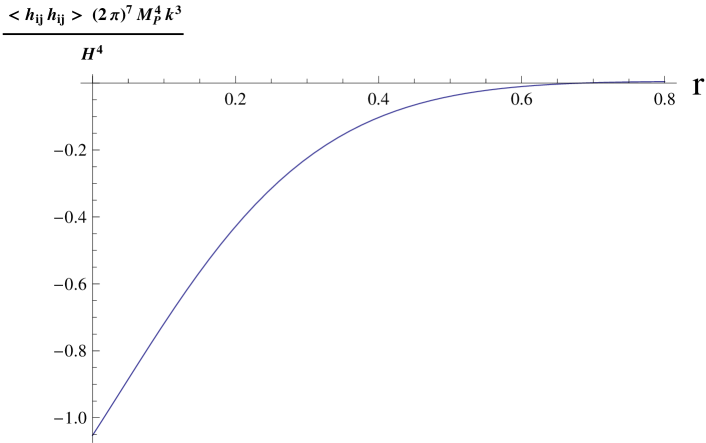
(a)

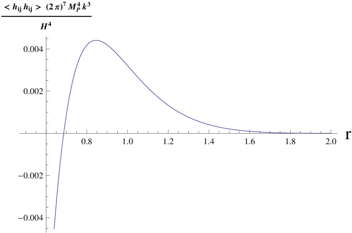
(b)

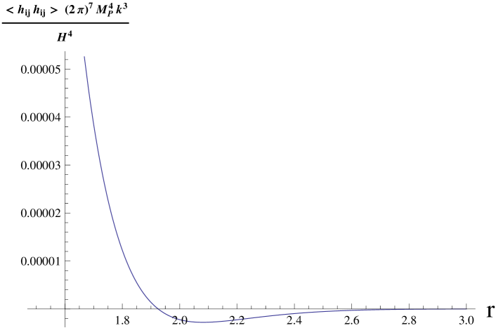
(c)

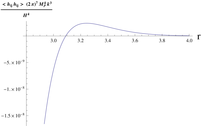
(d)

Figure 1: The $r$-dependence of Eq.(LABEL:powerspectrum4). We see that when $r\gtrsim 1$, the Dirac field may contribute negatively or positively to the power spectrum of gravitational wave, depending on the value of $r$, i.e. $m_{\psi}/H$.

From Fig.(1), we see that the $r$-dependent part is $\lesssim 1$, so the contribution of Dirac field to the gravitational wave power spectrum is $\simeq H^{4}/M_{P}^{4}$, which is scale-invariant. During inflation, the power spectrum of gravitational wave is $\simeq H^{2}/M_{P}^{2}$. Thus the contribution of spinor field is suppressed by the factor $H^{2}/M_{P}^{2}$. Additionally, from Fig.(1), we also observe that when $m_{\psi}\gtrsim H$, the $r$-dependent part has a nontrivial behavior, i.e. the Dirac field with different mass may contribute negatively or positively to the gravitational power spectrum which manifests itself from the negative or positive fermion loop correction.

The small mass limit $r\to 0$ of Eq.(LABEL:powerspectrum4) is interesting, since this case provides a maximal correction, which is

$$\langle h_{ij}(\mathbf{k})h_{ij}(\mathbf{k}^{\prime})\rangle|_{r\to 0}=\frac{\delta^{3}(\mathbf{k}-\mathbf{k^{\prime}})H^{4}}{(2\pi)^{7}M_{P}^{4}k^{3}}\left(-\frac{8\pi^{2}}{75}\right).$$ (21)

For a check, we follow Ref.[29], regulate the momentum integral by momentum cut-off, and replace the momentum integral and time integral as

$$\int d^{3}k\to\int^{\Lambda a(t1)}d^{3}k,\int_{-\infty}^{0}\tau^{\prime\prime}\int_{-\infty}^{0}\tau^{\prime}\to\int_{-\infty}^{0}d\tau^{\prime\prime}\int_{-\infty}^{\tau^{\prime\prime}(1+\frac{H}{\Lambda})}d\tau^{\prime},$$ (22)

where $\tau^{\prime}$ is the earlier one in time and $\Lambda$ is a physical cut-off. Since the associative cut-off in comoving momentum is time dependent, therefore we first integrate over momentum and then integrate over time. After taking the small mass limit $r\to 0$, we have

$$\langle h_{ij}(\mathbf{k})h_{ij}(\mathbf{k}^{\prime})\rangle_{r\to 0} = \frac{\delta^{3}(\mathbf{k}-\mathbf{k^{\prime}})\Lambda^{5}}{480\pi^{4}k^{3}HM_{P}^{4}(1+\frac{H}{\Lambda})^{4}}$$ (23)

$$-\frac{\delta^{3}(\mathbf{k}-\mathbf{k^{\prime}})H^{4}}{(2\pi)^{7}M_{P}^{4}k^{3}}\Big{(}\frac{64\pi^{2}(56+44\frac{H}{\Lambda}+18\frac{H^{2}}{\Lambda^{2}}+3\frac{H^{3}}{\Lambda^{3}})}{75(1+\frac{H}{\Lambda})^{4}(2+\frac{H}{\Lambda})^{3}}$$

$$-\frac{64\pi^{2}}{75}\frac{\Lambda^{3}(4+28\frac{H}{\Lambda}+78\frac{H^{2}}{\Lambda^{2}}+56\frac{H^{3}}{\Lambda^{3}}+44\frac{H^{4}}{\Lambda^{4}}+18\frac{H^{5}}{\Lambda^{5}}+3\frac{H^{6}}{\Lambda^{6}})}{H^{3}(1+\frac{H}{\Lambda})^{4}(2+\frac{H}{\Lambda})^{3}}$$

$$+\frac{64\pi^{3}\Lambda}{63H}-\frac{64\pi^{3}\Lambda^{3}}{105H^{3}}+\frac{8\pi^{3}\Lambda^{5}}{225H^{5}(1+\frac{H}{\Lambda})^{4}}\Big{)},$$

where the first line on the right-hand side of Eq. (23) comes from the $B$-part of Eq. (12), while the remaining parts of Eq. (23) come from the $A$-part of Eq. (12). We now leave behind the divergent terms $\sim\Lambda^{n},n\geq 1$ assuming that they can be reabsorbed by counter terms in renormalization process, and we get

$$\langle h_{ij}(\mathbf{k})h_{ij}(\mathbf{k}^{\prime})\rangle_{r\to 0} \sim -\frac{\delta^{3}(\mathbf{k}-\mathbf{k^{\prime}})H^{4}}{(2\pi)^{7}M_{P}^{4}k^{3}}\frac{64\pi^{2}(56+44\frac{H}{\Lambda}+18\frac{H^{2}}{\Lambda^{2}}+3\frac{H^{3}}{\Lambda^{3}})}{75(1+\frac{H}{\Lambda})^{4}(2+\frac{H}{\Lambda})^{3}}$$ (24)

$$= \left.-\frac{\delta^{3}(\mathbf{k}-\mathbf{k^{\prime}})H^{4}}{(2\pi)^{7}M_{P}^{4}k^{3}}\frac{64\times 56\pi^{2}}{75}\right|_{\frac{H}{\Lambda}\to 0}.$$

The above result shows the contribution induced by the Dirac field, in the small mass limit, is of the same order with Eq. (21).

Until now, the impact of quantum field renormalization on cosmological correlation functions is controversial. Some authors argued that the influence of renormalization can significantly change the predictions of slow-roll inflation for both scalar and tensor power spectra [30, 31, 32]. While some authors debated that the standard expression is valid and the UV regularisation leads to no difference in the bare power spectrum [33, 34, 35, 36, 37]. Though we focused on the effect of spinor field on the tensor power spectrum, similar case may also occur. However, the effect of spinor field is next-to-leading order, so we expect that available renormalization methods in literature do not alter our result in order of magnitude.

IV Conclusion

Gravity, being the weakest interaction, might provide abundant information about new physics in the very early universe directly. Due to the weakness in strength of gravity, it is very hard to detect the signals of gravitational waves. However, forthcoming experiments might soon be able to catch some sight of it. This motivates us to explore possible sources of primordial gravitational waves.

In this work, we studied the contribution of massive spinor field during inflation to the gravitational wave power spectrum by using retarded Green propagator. As an important step, we show the calculation process of spin sum for massive fermions in APPENDIX A. We worked out analytically the result for arbitrary mass $m_{\psi}$, and found that the correction is scale-invariant and of order $H^{4}/M_{P}^{4}$. Additionally, we also observe that when the mass of spinor field $m_{\psi}\gtrsim H$, depending on the value of $m_{\psi}$, the spinor field may contribute negatively or positively to the gravitational power spectrum.

The result obtained is actually far below the observational level, which is reasonable since they are of the second order in perturbation. And of course, we are only limited to the case with single spinor field, if there are lots of spinor fields, our result will multiply. In addition, it is also interesting to consider non-minimal coupling to gravity, e.g. non-minimal derivative coupling curvaton [38, 39], and things might be different. We leave this task to future work.

Acknowledgments

This work is supported by NSFC, No.11222546, and National Basic Research Program of China, No.2010CB832804.

Appendix A Trace

Equation Eq. (10) shows that the calculation of two point correlation function needs to sum over spins of massive fermions at different times. However, massive fermions in curved space are no longer conformally flat, and we can not use the spin sum formula from flat space. Here, we show the calculation process of this spin sum for massive fermions in great details. Despite the differences from the flat space, spin sum always leads to trace of some gamma matrices. the Fourier transformation of the fermion field is

$$\psi(\mathbf{x},t) = \int\mathrm{d}^{3}p\sum_{s}\left[e^{i\mathbf{p}\cdot\mathbf{x}}\alpha_{\mathbf{p},s}X_{\mathbf{p},s}(t)+e^{-i\mathbf{p}\cdot\mathbf{x}}\beta^{\dagger}_{\mathbf{p},s}W_{\mathbf{p},s}(t)\right]$$ (25)

$$= a^{-\frac{3}{2}}(t)\int\mathrm{d}^{3}p\sum_{s}\left[e^{i\mathbf{p}\cdot\mathbf{x}}\alpha_{\mathbf{p},s}u_{\mathbf{p},s}(t)+e^{-i\mathbf{p}\cdot\mathbf{x}}\beta^{\dagger}_{\mathbf{p},s}v_{\mathbf{p},s}(t)\right].$$

Namely,

$$X_{\mathbf{p},s}(t)\equiv a^{-\frac{3}{2}}(t)u_{\mathbf{p},s}(t),~{}W_{\mathbf{p},s}(t)\equiv a^{-\frac{3}{2}}(t)v_{\mathbf{p},s}(t).$$ (26)

We define

$$u_{s,\mathbf{p}}(\tau)\equiv\left(\begin{array}[]{c}u_{+,\mathbf{p}}(\tau)\psi_{s}\\ u_{-,\mathbf{p}}(\tau)\psi_{s}\end{array}\right);\quad v_{s,\mathbf{p}}(\tau)\equiv\left(\begin{array}[]{c}v_{+,\mathbf{p}}(\tau)\psi_{-s}\\ v_{-,\mathbf{p}}(\tau)\psi_{-s}\end{array}\right),$$ (31)

where $\psi_{+}=\left(\begin{array}[]{c}1\\ 0\end{array}\right)$ and $\psi_{-}=\left(\begin{array}[]{c}0\\ 1\end{array}\right)$ stand for spin up and down, respectively, which make $u_{s,\mathbf{p}}(\tau)$ and $v_{s,\mathbf{p}}(\tau)$ connected by charge conjugation as $v_{s,\mathbf{p}}(\tau)=C\bar{u}^{T}_{s,\mathbf{p}}(\tau)=C(u^{\dagger}\gamma^{0})^{T}=C\gamma^{0}u^{{\dagger}T}=C\gamma^{0}u^{*}$. Where

$$C=i\gamma^{0}\gamma^{2}=\left(\begin{array}[]{cc}0&i\sigma_{2}\\ i\sigma_{2}&0\end{array}\right)$$ (34)

is charge conjugation matrix. Then

$$\left(\begin{array}[]{c}v_{+,\mathbf{p}}(\tau)\psi_{-s}\\ v_{-,\mathbf{p}}(\tau)\psi_{-s}\end{array}\right) = \left(\begin{array}[]{cc}0&i\sigma_{2}\\ i\sigma_{2}&0\end{array}\right)\left(\begin{array}[]{cc}1&0\\ 0&-1\end{array}\right)\left(\begin{array}[]{c}u^{*}_{+,\mathbf{p}}(\tau)\psi_{s}\\ u^{*}_{-,\mathbf{p}}(\tau)\psi_{s}\end{array}\right)$$ (43)

$$= \left(\begin{array}[]{cc}0&-i\sigma_{2}\\ i\sigma_{2}&0\end{array}\right)\left(\begin{array}[]{c}u^{*}_{+,\mathbf{p}}(\tau)\psi_{s}\\ u^{*}_{-,\mathbf{p}}(\tau)\psi_{s}\end{array}\right)$$ (48)

$$= \left(\begin{array}[]{c}-i\sigma_{2}u^{*}_{-,\mathbf{p}}(\tau)\psi_{s}\\ i\sigma_{2}u^{*}_{+,\mathbf{p}}(\tau)\psi_{s}\end{array}\right).$$ (51)

Therefore

$$v_{+,\mathbf{p}}(\tau) = v_{+,\mathbf{p}}(\tau)\times\mathbf{1}_{2\times 2}=\sum_{s}v_{+,\mathbf{p}}(\tau)\psi_{-s}\psi^{T}_{-s}$$ (54)

$$= \sum_{s}(-i\sigma_{2})u^{*}_{-,\mathbf{p}}(\tau)\psi_{s}\psi^{T}_{-s}=(-i\sigma_{2})u^{*}_{-,\mathbf{p}}(\tau)\left(\begin{array}[]{cc}0&1\\ 1&0\end{array}\right)=-i\sigma_{2}u^{*}_{-,\mathbf{p}}(\tau)\sigma_{1},$$

$$v_{-,\mathbf{p}}(\tau) = v_{-,\mathbf{p}}(\tau)\times\mathbf{1}_{2\times 2}=\sum_{s}v_{-,\mathbf{p}}(\tau)\psi_{-s}\psi^{T}_{-s}$$ (57)

$$= \sum_{s}i\sigma_{2}u^{*}_{+,\mathbf{p}}(\tau)\psi_{s}\psi^{T}_{-s}=i\sigma_{2}u^{*}_{+,\mathbf{p}}(\tau)\left(\begin{array}[]{cc}0&1\\ 1&0\end{array}\right)=i\sigma_{2}u^{*}_{+,\mathbf{p}}(\tau)\sigma_{1}.$$

That is we have $v_{\pm,\mathbf{p}}(\tau)=\mp i\sigma_{2}u^{*}_{\mp,\mathbf{p}}(\tau)\sigma_{1}$. We can now calculate the spin sum.

$$\gamma^{m}_{ab}\gamma^{n}_{cd}\sum_{s}[\bar{W}_{\mathbf{p},s}(\tau^{\prime})]_{a}[W_{\mathbf{p},s}(\tau^{\prime\prime})]_{d}\sum_{s^{\prime}}[X_{\mathbf{p}^{\prime},s^{\prime}}(\tau^{\prime})]_{b}[\bar{X}_{\mathbf{p}^{\prime},s^{\prime}}(\tau^{\prime\prime})]_{c}$$ (58)

$$= \frac{1}{a^{3}(\tau^{\prime})a^{3}(\tau^{\prime\prime})}\sum_{s,s^{\prime}}\gamma^{m}_{ab}[u_{\mathbf{p}^{\prime},s^{\prime}}(\tau^{\prime})\bar{u}_{\mathbf{p}^{\prime},s^{\prime}}(\tau^{\prime\prime})]_{bc}\gamma^{n}_{cd}[v_{\mathbf{p},s}(\tau^{\prime\prime})\bar{v}_{\mathbf{p},s}(\tau^{\prime})]_{da}$$

$$= \frac{1}{a^{3}(\tau^{\prime})a^{3}(\tau^{\prime\prime})}\sum_{s,s^{\prime}}\mbox{tr}[\gamma^{m}u_{\mathbf{p}^{\prime},s^{\prime}}(\tau^{\prime})\bar{u}_{\mathbf{p}^{\prime},s^{\prime}}(\tau^{\prime\prime})\gamma^{n}v_{\mathbf{p},s}(\tau^{\prime\prime})\bar{v}_{\mathbf{p},s}(\tau^{\prime})],$$

The trace is

$$\sum_{s,s^{\prime}}\mbox{tr}[\gamma^{m}u_{\mathbf{p}^{\prime},s^{\prime}}(\tau^{\prime})\bar{u}_{\mathbf{p}^{\prime},s^{\prime}}(\tau^{\prime\prime})\gamma^{n}v_{\mathbf{p},s}(\tau^{\prime\prime})\bar{v}_{\mathbf{p},s}(\tau^{\prime})]$$ (63)

$$= \sum_{s,s^{\prime}}\mbox{tr}[\gamma^{m}u_{\mathbf{p}^{\prime},s^{\prime}}(\tau^{\prime})u^{\dagger}_{\mathbf{p}^{\prime},s^{\prime}}(\tau^{\prime\prime})\gamma^{0}\gamma^{n}v_{\mathbf{p},s}(\tau^{\prime\prime})v^{\dagger}_{\mathbf{p},s}(\tau^{\prime})\gamma^{0}]$$

$$= \sum_{s,s^{\prime}}\mbox{tr}[\left(\begin{array}[]{cc}0&\sigma_{m}\\ \sigma_{m}&0\end{array}\right)\left(\begin{array}[]{c}u_{+,\mathbf{p}^{\prime}}(\tau^{\prime})\psi_{s^{\prime}}\\ u_{-,\mathbf{p}^{\prime}}(\tau^{\prime})\psi_{s^{\prime}}\end{array}\right)\left(\psi_{s^{\prime}}^{T}u^{\dagger}_{+,\mathbf{p}^{\prime}}(\tau^{\prime\prime}),\psi_{s^{\prime}}^{T}u^{\dagger}_{-,\mathbf{p}^{\prime}}(\tau^{\prime\prime})\right)$$

$$\left(\begin{array}[]{cc}0&\sigma_{n}\\ \sigma_{n}&0\end{array}\right)\left(\begin{array}[]{c}v_{+,\mathbf{p}}(\tau^{\prime\prime})\psi_{-s}\\ v_{-,\mathbf{p}}(\tau^{\prime\prime})\psi_{-s}\end{array}\right)\left(\psi_{-s}^{T}v^{\dagger}_{+,\mathbf{p}}(\tau^{\prime}),\psi_{-s}^{T}v^{\dagger}_{-,\mathbf{p}}(\tau^{\prime})\right)]$$ (68)

$$= \sum_{s,s^{\prime}}\mbox{tr}[\left(\begin{array}[]{cc}0&\sigma_{m}\\ \sigma_{m}&0\end{array}\right)\left(\begin{array}[]{cc}u_{+,\mathbf{p}^{\prime}}(\tau^{\prime})\psi_{s^{\prime}}\psi_{s^{\prime}}^{T}u^{\dagger}_{+,\mathbf{p}^{\prime}}(\tau^{\prime\prime})&u_{+,\mathbf{p}^{\prime}}(\tau^{\prime})\psi_{s^{\prime}}\psi_{s^{\prime}}^{T}u^{\dagger}_{-,\mathbf{p}^{\prime}}(\tau^{\prime\prime})\\ u_{-,\mathbf{p}^{\prime}}(\tau^{\prime})\psi_{s^{\prime}}\psi_{s^{\prime}}^{T}u^{\dagger}_{+,\mathbf{p}^{\prime}}(\tau^{\prime\prime})&u_{-,\mathbf{p}^{\prime}}(\tau^{\prime})\psi_{s^{\prime}}\psi_{s^{\prime}}^{T}u^{\dagger}_{-,\mathbf{p}^{\prime}}(\tau^{\prime\prime})\end{array}\right)$$ (73)

$$\left(\begin{array}[]{cc}0&\sigma_{n}\\ \sigma_{n}&0\end{array}\right)\left(\begin{array}[]{cc}v_{+,\mathbf{p}}(\tau^{\prime\prime})\psi_{-s}\psi_{-s}^{T}v^{\dagger}_{+,\mathbf{p}}(\tau^{\prime})&v_{+,\mathbf{p}}(\tau^{\prime\prime})\psi_{-s}\psi_{-s}^{T}v^{\dagger}_{-,\mathbf{p}}(\tau^{\prime})\\ v_{-,\mathbf{p}}(\tau^{\prime\prime})\psi_{-s}\psi_{-s}^{T}v^{\dagger}_{+,\mathbf{p}}(\tau^{\prime})&v_{-,\mathbf{p}}(\tau^{\prime\prime})\psi_{-s}\psi_{-s}^{T}v^{\dagger}_{-,\mathbf{p}}(\tau^{\prime})\end{array}\right)],$$ (78)

while

$$\sum_{s=\pm}\psi_{s}\psi_{s}^{T}=\left(\begin{array}[]{c}0\\ 1\end{array}\right)(0,1)+\left(\begin{array}[]{c}1\\ 0\end{array}\right)(1,0)=\left(\begin{array}[]{cc}1&0\\ 0&1\end{array}\right).$$ (85)

Therefore we have

$$\sum_{s,s^{\prime}}\mbox{tr}[\gamma^{m}u_{\mathbf{p}^{\prime},s^{\prime}}(\tau^{\prime})\bar{u}_{\mathbf{p}^{\prime},s^{\prime}}(\tau^{\prime\prime})\gamma^{n}v_{\mathbf{p},s}(\tau^{\prime\prime})\bar{v}_{\mathbf{p},s}(\tau^{\prime})]$$ (90)

$$= \mbox{tr}[\left(\begin{array}[]{cc}0&\sigma_{m}\\ \sigma_{m}&0\end{array}\right)\left(\begin{array}[]{cc}u_{+,\mathbf{p}^{\prime}}(\tau^{\prime})u^{\dagger}_{+,\mathbf{p}^{\prime}}(\tau^{\prime\prime})&u_{+,\mathbf{p}^{\prime}}(\tau^{\prime})u^{\dagger}_{-,\mathbf{p}^{\prime}}(\tau^{\prime\prime})\\ u_{-,\mathbf{p}^{\prime}}(\tau^{\prime})u^{\dagger}_{+,\mathbf{p}^{\prime}}(\tau^{\prime\prime})&u_{-,\mathbf{p}^{\prime}}(\tau^{\prime})u^{\dagger}_{-,\mathbf{p}^{\prime}}(\tau^{\prime\prime})\end{array}\right)$$

$$\left(\begin{array}[]{cc}0&\sigma_{n}\\ \sigma_{n}&0\end{array}\right)\left(\begin{array}[]{cc}v_{+,\mathbf{p}}(\tau^{\prime\prime})v^{\dagger}_{+,\mathbf{p}}(\tau^{\prime})&v_{+,\mathbf{p}}(\tau^{\prime\prime})v^{\dagger}_{-,\mathbf{p}}(\tau^{\prime})\\ v_{-,\mathbf{p}}(\tau^{\prime\prime})v^{\dagger}_{+,\mathbf{p}}(\tau^{\prime})&v_{-,\mathbf{p}}(\tau^{\prime\prime})v^{\dagger}_{-,\mathbf{p}}(\tau^{\prime})\end{array}\right)]$$ (95)

$$= \mbox{tr}[\left(\begin{array}[]{cc}\sigma_{m}u_{-,\mathbf{p}^{\prime}}(\tau^{\prime})u^{\dagger}_{+,\mathbf{p}^{\prime}}(\tau^{\prime\prime})&\sigma_{m}u_{-,\mathbf{p}^{\prime}}(\tau^{\prime})u^{\dagger}_{-,\mathbf{p}^{\prime}}(\tau^{\prime\prime})\\ \sigma_{m}u_{+,\mathbf{p}^{\prime}}(\tau^{\prime})u^{\dagger}_{+,\mathbf{p}^{\prime}}(\tau^{\prime\prime})&\sigma_{m}u_{+,\mathbf{p}^{\prime}}(\tau^{\prime})u^{\dagger}_{-,\mathbf{p}^{\prime}}(\tau^{\prime\prime})\end{array}\right)$$ (98)

$$\left(\begin{array}[]{cc}\sigma_{n}v_{-,\mathbf{p}}(\tau^{\prime\prime})v^{\dagger}_{+,\mathbf{p}}(\tau^{\prime})&\sigma_{n}v_{-,\mathbf{p}}(\tau^{\prime\prime})v^{\dagger}_{-,\mathbf{p}}(\tau^{\prime})\\ \sigma_{n}v_{+,\mathbf{p}}(\tau^{\prime\prime})v^{\dagger}_{+,\mathbf{p}}(\tau^{\prime})&\sigma_{n}v_{+,\mathbf{p}}(\tau^{\prime\prime})v^{\dagger}_{-,\mathbf{p}}(\tau^{\prime})\end{array}\right)]$$

$$= \mbox{tr}[\sigma_{m}u_{-,\mathbf{p}^{\prime}}(\tau^{\prime})u^{\dagger}_{+,\mathbf{p}^{\prime}}(\tau^{\prime\prime})\sigma_{n}v_{-,\mathbf{p}}(\tau^{\prime\prime})v^{\dagger}_{+,\mathbf{p}}(\tau^{\prime})+\sigma_{m}u_{-,\mathbf{p}^{\prime}}(\tau^{\prime})u^{\dagger}_{-,\mathbf{p}^{\prime}}(\tau^{\prime\prime})\sigma_{n}v_{+,\mathbf{p}}(\tau^{\prime\prime})v^{\dagger}_{+,\mathbf{p}}(\tau^{\prime})$$

$$+\sigma_{m}u_{+,\mathbf{p}^{\prime}}(\tau^{\prime})u^{\dagger}_{+,\mathbf{p}^{\prime}}(\tau^{\prime\prime})\sigma_{n}v_{-,\mathbf{p}}(\tau^{\prime\prime})v^{\dagger}_{-,\mathbf{p}}(\tau^{\prime})+\sigma_{m}u_{+,\mathbf{p}^{\prime}}(\tau^{\prime})u^{\dagger}_{-,\mathbf{p}^{\prime}}(\tau^{\prime\prime})\sigma_{n}v_{+,\mathbf{p}}(\tau^{\prime\prime})v^{\dagger}_{-,\mathbf{p}}(\tau^{\prime})]$$

$$= \mbox{tr}[-\sigma_{m}u_{-,\mathbf{p}^{\prime}}(\tau^{\prime})u^{\dagger}_{+,\mathbf{p}^{\prime}}(\tau^{\prime\prime})\sigma_{n}\sigma_{2}u^{*}_{+,\mathbf{p}}(\tau^{\prime\prime})u^{T}_{-,\mathbf{p}}(\tau^{\prime})\sigma_{2}^{\dagger}+\sigma_{m}u_{-,\mathbf{p}^{\prime}}(\tau^{\prime})u^{\dagger}_{-,\mathbf{p}^{\prime}}(\tau^{\prime\prime})\sigma_{n}\sigma_{2}u^{*}_{-,\mathbf{p}}(\tau^{\prime\prime})u^{T}_{-,\mathbf{p}}(\tau^{\prime})\sigma_{2}^{\dagger}$$

$$+\sigma_{m}u_{+,\mathbf{p}^{\prime}}(\tau^{\prime})u^{\dagger}_{+,\mathbf{p}^{\prime}}(\tau^{\prime\prime})\sigma_{n}\sigma_{2}u^{*}_{+,\mathbf{p}}(\tau^{\prime\prime})u^{T}_{+,\mathbf{p}}(\tau^{\prime})\sigma_{2}^{\dagger}-\sigma_{m}u_{+,\mathbf{p}^{\prime}}(\tau^{\prime})u^{\dagger}_{-,\mathbf{p}^{\prime}}(\tau^{\prime\prime})\sigma_{n}\sigma_{2}u^{*}_{-,\mathbf{p}}(\tau^{\prime\prime})u^{T}_{+,\mathbf{p}}(\tau^{\prime})\sigma_{2}^{\dagger}],$$

where we have used $v_{\pm,\mathbf{p}}(\tau)=\mp i\sigma_{2}u^{*}_{\mp,\mathbf{p}}(\tau)\sigma_{1}$. The solutions are

$$u_{s,\mathbf{p}}(\tau)\equiv\left(\begin{array}[]{c}u_{\mu,\mathbf{p}}(\tau)\times\psi_{s}\\ (\hat{p}\cdot\mathbf{\sigma})u_{\bar{\mu},\mathbf{p}}(\tau)\times\psi_{s}\end{array}\right),$$ (105)

with

$$u_{+,\mathbf{p}^{\prime}}(\tau^{\prime})=\mathbf{1}_{2\times 2}u_{\mu,\mathbf{p}}(\tau),$$ (106)

$$u_{+,\mathbf{p}^{\prime}}(\tau^{\prime})=(\hat{p}\cdot\mathbf{\sigma})u_{\bar{\mu},\mathbf{p}}(\tau),$$ (107)

where $\mu\equiv\frac{1}{2}-ir,\quad\bar{\mu}\equiv\frac{1}{2}+ir$ and

$$u_{\mu}(x)=\frac{i\sqrt{\pi x}}{2(2\pi)^{3/2}}e^{\frac{\pi r}{2}}H_{\mu}^{(1)}(x),$$ (108)

$$u_{\bar{\mu}}(x)=\frac{i\sqrt{\pi x}}{2(2\pi)^{3/2}}e^{-\frac{\pi r}{2}}H_{\bar{\mu}}^{(1)}(x).$$ (109)

Hankel function goes as

$$H_{\beta}^{(1)}\simeq-\frac{i\Gamma(\beta)}{\pi}\left(\frac{x}{2}\right)^{-\beta},\quad x\ll 1,\beta>0,$$ (110)

in small $x$ limit. Therefore in this situation, the mode functions behave like

$$u_{\mu}(x)\simeq\frac{\Gamma(\mu)e^{\frac{\pi r}{2}}}{(2\pi)^{2}}\left(\frac{x}{2}\right)^{ir},$$ (111)

$$u_{\bar{\mu}}(x)\simeq\frac{\Gamma(\bar{\mu})e^{-\frac{\pi r}{2}}}{(2\pi)^{2}}\left(\frac{x}{2}\right)^{-ir}.$$ (112)

Then we have

$$\sum_{s,s^{\prime}}\mbox{tr}[\gamma^{m}u_{\mathbf{p}^{\prime},s^{\prime}}(\tau^{\prime})\bar{u}_{\mathbf{p}^{\prime},s^{\prime}}(\tau^{\prime\prime})\gamma^{n}v_{\mathbf{p},s}(\tau^{\prime\prime})\bar{v}_{\mathbf{p},s}(\tau^{\prime})]$$ (113)

$$= \mbox{tr}[-\sigma_{m}u_{-,\mathbf{p}^{\prime}}(\tau^{\prime})u^{\dagger}_{+,\mathbf{p}^{\prime}}(\tau^{\prime\prime})\sigma_{n}\sigma_{2}u^{*}_{+,\mathbf{p}}(\tau^{\prime\prime})u^{T}_{-,\mathbf{p}}(\tau^{\prime})\sigma_{2}^{\dagger}+\sigma_{m}u_{-,\mathbf{p}^{\prime}}(\tau^{\prime})u^{\dagger}_{-,\mathbf{p}^{\prime}}(\tau^{\prime\prime})\sigma_{n}\sigma_{2}u^{*}_{-,\mathbf{p}}(\tau^{\prime\prime})u^{T}_{-,\mathbf{p}}(\tau^{\prime})\sigma_{2}^{\dagger}$$

$$+\sigma_{m}u_{+,\mathbf{p}^{\prime}}(\tau^{\prime})u^{\dagger}_{+,\mathbf{p}^{\prime}}(\tau^{\prime\prime})\sigma_{n}\sigma_{2}u^{*}_{+,\mathbf{p}}(\tau^{\prime\prime})u^{T}_{+,\mathbf{p}}(\tau^{\prime})\sigma_{2}^{\dagger}-\sigma_{m}u_{+,\mathbf{p}^{\prime}}(\tau^{\prime})u^{\dagger}_{-,\mathbf{p}^{\prime}}(\tau^{\prime\prime})\sigma_{n}\sigma_{2}u^{*}_{-,\mathbf{p}}(\tau^{\prime\prime})u^{T}_{+,\mathbf{p}}(\tau^{\prime})\sigma_{2}^{\dagger}]$$

$$= \mbox{tr}[-\sigma_{m}(\hat{p}^{\prime}\cdot\mathbf{\sigma})u_{\bar{\mu},\mathbf{p}^{\prime}}(\tau^{\prime})u^{*}_{\mu,\mathbf{p}^{\prime}}(\tau^{\prime\prime})\sigma_{n}\sigma_{2}u^{*}_{\mu,\mathbf{p}}(\tau^{\prime\prime})(\hat{p}\cdot\mathbf{\sigma})^{T}u_{\bar{\mu},\mathbf{p}}(\tau^{\prime})\sigma_{2}^{\dagger}$$

$$+\sigma_{m}(\hat{p}^{\prime}\cdot\mathbf{\sigma})u_{\bar{\mu},\mathbf{p}^{\prime}}(\tau^{\prime})(\hat{p}^{\prime}\cdot\mathbf{\sigma})^{\dagger}u^{*}_{\bar{\mu},\mathbf{p}^{\prime}}(\tau^{\prime\prime})\sigma_{n}\sigma_{2}(\hat{p}\cdot\mathbf{\sigma})^{*}u^{*}_{\bar{\mu},\mathbf{p}}(\tau^{\prime\prime})(\hat{p}\cdot\mathbf{\sigma})^{T}u_{\bar{\mu},\mathbf{p}}(\tau^{\prime})\sigma_{2}^{\dagger}$$

$$+\sigma_{m}u_{\mu,\mathbf{p}^{\prime}}(\tau^{\prime})u^{*}_{\mu,\mathbf{p}^{\prime}}(\tau^{\prime\prime})\sigma_{n}\sigma_{2}u^{*}_{\mu,\mathbf{p}}(\tau^{\prime\prime})u_{\mu,\mathbf{p}}(\tau^{\prime})\sigma_{2}^{\dagger}$$

$$-\sigma_{m}u_{\mu,\mathbf{p}^{\prime}}(\tau^{\prime})(\hat{p}^{\prime}\cdot\mathbf{\sigma})^{\dagger}u^{*}_{\bar{\mu},\mathbf{p}^{\prime}}(\tau^{\prime\prime})\sigma_{n}\sigma_{2}(\hat{p}\cdot\mathbf{\sigma})^{*}u^{*}_{\bar{\mu},\mathbf{p}}(\tau^{\prime\prime})u_{\mu,\mathbf{p}}(\tau^{\prime})\sigma_{2}^{\dagger}]$$

$$= \mbox{tr}[-\sigma_{m}(\hat{p}^{\prime}\cdot\mathbf{\sigma})\sigma_{n}\sigma_{2}(\hat{p}\cdot\mathbf{\sigma})^{T}\sigma_{2}^{\dagger}u_{\bar{\mu},\mathbf{p}^{\prime}}(\tau^{\prime})u^{*}_{\mu,\mathbf{p}^{\prime}}(\tau^{\prime\prime})u^{*}_{\mu,\mathbf{p}}(\tau^{\prime\prime})u_{\bar{\mu},\mathbf{p}}(\tau^{\prime})$$

$$+\sigma_{m}(\hat{p}^{\prime}\cdot\mathbf{\sigma})(\hat{p}^{\prime}\cdot\mathbf{\sigma})^{\dagger}\sigma_{n}\sigma_{2}(\hat{p}\cdot\mathbf{\sigma})^{*}(\hat{p}\cdot\mathbf{\sigma})^{T}\sigma_{2}^{\dagger}u_{\bar{\mu},\mathbf{p}^{\prime}}(\tau^{\prime})u^{*}_{\bar{\mu},\mathbf{p}^{\prime}}(\tau^{\prime\prime})u^{*}_{\bar{\mu},\mathbf{p}}(\tau^{\prime\prime})u_{\bar{\mu},\mathbf{p}}(\tau^{\prime})$$

$$+\sigma_{m}\sigma_{n}\sigma_{2}\sigma_{2}^{\dagger}u_{\mu,\mathbf{p}^{\prime}}(\tau^{\prime})u^{*}_{\mu,\mathbf{p}^{\prime}}(\tau^{\prime\prime})u^{*}_{\mu,\mathbf{p}}(\tau^{\prime\prime})u_{\mu,\mathbf{p}}(\tau^{\prime})$$

$$-\sigma_{m}(\hat{p}^{\prime}\cdot\mathbf{\sigma})^{\dagger}\sigma_{n}\sigma_{2}(\hat{p}\cdot\mathbf{\sigma})^{*}\sigma_{2}^{\dagger}u_{\mu,\mathbf{p}^{\prime}}(\tau^{\prime})u^{*}_{\bar{\mu},\mathbf{p}^{\prime}}(\tau^{\prime\prime})u^{*}_{\bar{\mu},\mathbf{p}}(\tau^{\prime\prime})u_{\mu,\mathbf{p}}(\tau^{\prime})]$$

$$= \mbox{tr}[\sigma_{m}(\hat{p}^{\prime}\cdot\mathbf{\sigma})\sigma_{n}(\hat{p}\cdot\mathbf{\sigma})u_{\bar{\mu},\mathbf{p}^{\prime}}(\tau^{\prime})u^{*}_{\mu,\mathbf{p}^{\prime}}(\tau^{\prime\prime})u^{*}_{\mu,\mathbf{p}}(\tau^{\prime\prime})u_{\bar{\mu},\mathbf{p}}(\tau^{\prime})$$

$$+\sigma_{m}\sigma_{n}u_{\bar{\mu},\mathbf{p}^{\prime}}(\tau^{\prime})u^{*}_{\bar{\mu},\mathbf{p}^{\prime}}(\tau^{\prime\prime})u^{*}_{\bar{\mu},\mathbf{p}}(\tau^{\prime\prime})u_{\bar{\mu},\mathbf{p}}(\tau^{\prime})$$

$$+\sigma_{m}\sigma_{n}u_{\mu,\mathbf{p}^{\prime}}(\tau^{\prime})u^{*}_{\mu,\mathbf{p}^{\prime}}(\tau^{\prime\prime})u^{*}_{\mu,\mathbf{p}}(\tau^{\prime\prime})u_{\mu,\mathbf{p}}(\tau^{\prime})$$

$$+\sigma_{m}(\hat{p}^{\prime}\cdot\mathbf{\sigma})^{\dagger}\sigma_{n}(\hat{p}\cdot\mathbf{\sigma})u_{\mu,\mathbf{p}^{\prime}}(\tau^{\prime})u^{*}_{\bar{\mu},\mathbf{p}^{\prime}}(\tau^{\prime\prime})u^{*}_{\bar{\mu},\mathbf{p}}(\tau^{\prime\prime})u_{\mu,\mathbf{p}}(\tau^{\prime})],$$

where we have use

$$(\hat{p}\cdot\mathbf{\sigma})(\hat{p}\cdot\mathbf{\sigma})^{\dagger}=\left(\begin{array}[]{cc}\hat{p}_{3}&\hat{p}_{1}-i\hat{p}_{2}\\ \hat{p}_{1}+i\hat{p}_{2}&-\hat{p}_{3}\end{array}\right)\left(\begin{array}[]{cc}\hat{p}_{3}&\hat{p}_{1}-i\hat{p}_{2}\\ \hat{p}_{1}+i\hat{p}_{2}&-\hat{p}_{3}\end{array}\right)=(\hat{p}_{1}^{2}+\hat{p}_{2}^{2}+\hat{p}_{3}^{2})\mathbf{1}_{2\times 2},$$ (118)

$$(\hat{p}\cdot\mathbf{\sigma})^{*}(\hat{p}\cdot\mathbf{\sigma})^{T}=[(\hat{p}^{\prime}\cdot\mathbf{\sigma})(\hat{p}^{\prime}\cdot\mathbf{\sigma})^{\dagger}]^{*}=\mathbf{1}_{2\times 2},$$ (119)

$$\sigma_{2}(\hat{p}\cdot\mathbf{\sigma})^{T}\sigma_{2}^{\dagger}=\sigma_{2}(\hat{p}\cdot\mathbf{\sigma})^{*}\sigma_{2}^{\dagger}=-\hat{p}\cdot\mathbf{\sigma},$$ (120)

while

$$u_{\bar{\mu},\mathbf{p}^{\prime}}(\tau^{\prime})u^{*}_{\mu,\mathbf{p}^{\prime}}(\tau^{\prime\prime})u^{*}_{\mu,\mathbf{p}}(\tau^{\prime\prime})u_{\bar{\mu},\mathbf{p}}(\tau^{\prime})$$

$$= \frac{\Gamma(\bar{\mu})\Gamma^{*}(\mu)\Gamma^{*}(\mu)\Gamma(\bar{\mu})}{(2\pi)^{8}}\left(\frac{-p^{\prime}\tau^{\prime}}{2}\right)^{-ir}\left(\frac{-p^{\prime}\tau^{\prime\prime}}{2}\right)^{-ir}\left(\frac{-p\tau^{\prime\prime}}{2}\right)^{-ir}\left(\frac{-p\tau^{\prime}}{2}\right)^{-ir}$$

$$= \frac{\Gamma^{4}(\bar{\mu})}{(2\pi)^{8}}\left(\frac{-p^{\prime}\tau^{\prime}}{2}\right)^{-2ir}\left(\frac{-p\tau^{\prime\prime}}{2}\right)^{-2ir},$$

$$u_{\mu,\mathbf{p}^{\prime}}(\tau^{\prime})u^{*}_{\bar{\mu},\mathbf{p}^{\prime}}(\tau^{\prime\prime})u^{*}_{\bar{\mu},\mathbf{p}}(\tau^{\prime\prime})u_{\mu,\mathbf{p}}(\tau^{\prime})$$

$$= \frac{\Gamma(\mu)\Gamma^{*}(\bar{\mu})\Gamma^{*}(\bar{\mu})\Gamma(\mu)}{(2\pi)^{8}}\left(\frac{-p^{\prime}\tau^{\prime}}{2}\right)^{ir}\left(\frac{-p^{\prime}\tau^{\prime\prime}}{2}\right)^{ir}\left(\frac{-p\tau^{\prime\prime}}{2}\right)^{ir}\left(\frac{-p\tau^{\prime}}{2}\right)^{ir}$$

$$= \frac{\Gamma^{4}(\mu)}{(2\pi)^{8}}\left(\frac{-p^{\prime}\tau^{\prime}}{2}\right)^{2ir}\left(\frac{-p\tau^{\prime\prime}}{2}\right)^{2ir},$$ (122)

and

$$u_{\bar{\mu},\mathbf{p}^{\prime}}(\tau^{\prime})u^{*}_{\bar{\mu},\mathbf{p}^{\prime}}(\tau^{\prime\prime})u^{*}_{\bar{\mu},\mathbf{p}}(\tau^{\prime\prime})u_{\bar{\mu},\mathbf{p}}(\tau^{\prime})$$

$$= \frac{\Gamma(\bar{\mu})\Gamma^{*}(\bar{\mu})\Gamma^{*}(\bar{\mu})\Gamma(\bar{\mu})}{(2\pi)^{8}}e^{-2\pi r}\left(\frac{-p^{\prime}\tau^{\prime}}{2}\right)^{-ir}\left(\frac{-p^{\prime}\tau^{\prime\prime}}{2}\right)^{ir}\left(\frac{-p\tau^{\prime\prime}}{2}\right)^{ir}\left(\frac{-p\tau^{\prime}}{2}\right)^{-ir}$$

$$= \frac{|\Gamma(\bar{\mu})|^{4}}{(2\pi)^{8}}e^{-2\pi r}\tau^{\prime-2ir}\tau^{\prime\prime 2ir},$$

$$u_{\mu,\mathbf{p}^{\prime}}(\tau^{\prime})u^{*}_{\mu,\mathbf{p}^{\prime}}(\tau^{\prime\prime})u^{*}_{\mu,\mathbf{p}}(\tau^{\prime\prime})u_{\mu,\mathbf{p}}(\tau^{\prime})$$

$$= \frac{\Gamma(\mu)\Gamma^{*}(\mu)\Gamma^{*}(\mu)\Gamma(\mu)}{(2\pi)^{8}}e^{2\pi r}\left(\frac{-p^{\prime}\tau^{\prime}}{2}\right)^{ir}\left(\frac{-p^{\prime}\tau^{\prime\prime}}{2}\right)^{-ir}\left(\frac{-p\tau^{\prime\prime}}{2}\right)^{-ir}\left(\frac{-p\tau^{\prime}}{2}\right)^{ir}$$

$$= \frac{|\Gamma(\mu)|^{4}}{(2\pi)^{8}}e^{2\pi r}\tau^{\prime 2ir}\tau^{\prime\prime-2ir}.$$ (124)

Finally, we get

$$\sum_{s,s^{\prime}}\mbox{tr}[\gamma^{m}u_{\mathbf{p}^{\prime},s^{\prime}}(\tau^{\prime})\bar{u}_{\mathbf{p}^{\prime},s^{\prime}}(\tau^{\prime\prime})\gamma^{n}v_{\mathbf{p},s}(\tau^{\prime\prime})\bar{v}_{\mathbf{p},s}(\tau^{\prime})]$$ (125)

$$= \mbox{tr}[\sigma_{m}(\hat{p}^{\prime}\cdot\mathbf{\sigma})\sigma_{n}(\hat{p}\cdot\mathbf{\sigma})u_{\bar{\mu},\mathbf{p}^{\prime}}(\tau^{\prime})u^{*}_{\mu,\mathbf{p}^{\prime}}(\tau^{\prime\prime})u^{*}_{\mu,\mathbf{p}}(\tau^{\prime\prime})u_{\bar{\mu},\mathbf{p}}(\tau^{\prime})$$

$$+\sigma_{m}\sigma_{n}u_{\bar{\mu},\mathbf{p}^{\prime}}(\tau^{\prime})u^{*}_{\bar{\mu},\mathbf{p}^{\prime}}(\tau^{\prime\prime})u^{*}_{\bar{\mu},\mathbf{p}}(\tau^{\prime\prime})u_{\bar{\mu},\mathbf{p}}(\tau^{\prime})$$

$$+\sigma_{m}\sigma_{n}u_{\mu,\mathbf{p}^{\prime}}(\tau^{\prime})u^{*}_{\mu,\mathbf{p}^{\prime}}(\tau^{\prime\prime})u^{*}_{\mu,\mathbf{p}}(\tau^{\prime\prime})u_{\mu,\mathbf{p}}(\tau^{\prime})$$

$$+\sigma_{m}(\hat{p}^{\prime}\cdot\mathbf{\sigma})^{\dagger}\sigma_{n}(\hat{p}\cdot\mathbf{\sigma})u_{\mu,\mathbf{p}^{\prime}}(\tau^{\prime})u^{*}_{\bar{\mu},\mathbf{p}^{\prime}}(\tau^{\prime\prime})u^{*}_{\bar{\mu},\mathbf{p}}(\tau^{\prime\prime})u_{\mu,\mathbf{p}}(\tau^{\prime})]$$

$$= \mbox{tr}[\sigma_{m}(\hat{p}^{\prime}\cdot\mathbf{\sigma})\sigma_{n}(\hat{p}\cdot\mathbf{\sigma})](\frac{\Gamma^{4}(\bar{\mu})}{(2\pi)^{8}}\left(\frac{-p^{\prime}\tau^{\prime}}{2}\right)^{-2ir}\left(\frac{-p\tau^{\prime\prime}}{2}\right)^{-2ir}+\frac{\Gamma^{4}(\mu)}{(2\pi)^{8}}\left(\frac{-p^{\prime}\tau^{\prime}}{2}\right)^{2ir}\left(\frac{-p\tau^{\prime\prime}}{2}\right)^{2ir})$$

$$+\mbox{tr}[\sigma_{m}\sigma_{n}](\frac{|\Gamma(\bar{\mu})|^{4}}{(2\pi)^{8}}e^{-2\pi r}\tau^{\prime-2ir}\tau^{\prime\prime 2ir}+\frac{|\Gamma(\mu)|^{4}}{(2\pi)^{8}}e^{2\pi r}\tau^{\prime 2ir}\tau^{\prime\prime-2ir}).$$

References

- [1] D. Baumann et al. [CMBPol Study Team Collaboration], AIP Conf. Proc. 1141, 10 (2009) [arXiv:0811.3919 [astro-ph]].
- [2] P. A. R. Ade et al. [BICEP2 Collaboration], Phys. Rev. Lett. 112, 241101 (2014) [arXiv:1403.3985 [astro-ph.CO]].
- [3] L. P. Grishchuk, Sov. Phys. JETP 40, 409 (1975).
- [4] A. A. Starobinsky, JETP Lett. 30, 682 (1979).
- [5] V. A. Rubakov, M. V. Sazhin, and A. V. Veryaskin, Phys. Lett. B115, 189 (1982).
- [6] Y. Cai, Y. T. Wang and Y. S. Piao, Phys. Rev. D 91, 103001 (2015) [arXiv:1501.06345 [astro-ph.CO]].
- [7] T. Damour and A. Vilenkin, Phys. Rev. Lett. 85, 3761 (2000) [gr-qc/0004075].
- [8] D. G. Figueroa, M. Hindmarsh and J. Urrestilla, Phys. Rev. Lett. 110, no. 10, 101302 (2013) [arXiv:1212.5458 [astro-ph.CO]].
- [9] A. Kosowsky, M. S. Turner and R. Watkins, Phys. Rev. D 45, 4514 (1992).
- [10] M. Kamionkowski, A. Kosowsky and M. S. Turner, Phys. Rev. D 49, 2837 (1994) [astro-ph/9310044].
- [11] X. Chen and Y. Wang, JCAP 1004, 027 (2010) [arXiv:0911.3380 [hep-th]].
- [12] X. Chen and Y. Wang, JCAP 1209, 021 (2012) [arXiv:1205.0160 [hep-th]].
- [13] A. Kehagias and A. Riotto, Fortsch. Phys. 63, 531 (2015) [arXiv:1501.03515 [hep-th]].
- [14] N. Arkani-Hamed and J. Maldacena, arXiv:1503.08043 [hep-th].
- [15] E. Dimastrogiovanni, M. Fasiello and M. Kamionkowski, arXiv:1504.05993 [astro-ph.CO].
- [16] M. Biagetti, M. Fasiello and A. Riotto, Phys. Rev. D 88, no. 10, 103518 (2013) [arXiv:1305.7241 [astro-ph.CO]].
- [17] M. Biagetti, E. Dimastrogiovanni, M. Fasiello and M. Peloso, JCAP 1504, 011 (2015) [arXiv:1411.3029 [astro-ph.CO]].
- [18] T. Fujita, J. Yokoyama and S. Yokoyama, PTEP 2015, 043E01 (2015) [arXiv:1411.3658 [astro-ph.CO]].
- [19] J. L. Cook and L. Sorbo, Phys. Rev. D 85, 023534 (2012) [Erratum-ibid. D 86, 069901 (2012)] [arXiv:1109.0022 [astro-ph.CO]].
- [20] N. Barnaby, J. Moxon, R. Namba, M. Peloso, G. Shiu and P. Zhou, Phys. Rev. D 86, 103508 (2012) [arXiv:1206.6117 [astro-ph.CO]].
- [21] D. J. H. Chung, E. W. Kolb, A. Riotto and I. I. Tkachev, Phys. Rev. D 62, 043508 (2000) [hep-ph/9910437].
- [22] D. G. Figueroa and T. Meriniemi, JHEP 1310, 101 (2013) [arXiv:1306.6911 [astro-ph.CO]].
- [23] S. Weinberg, Phys. Rev. D 72, 043514 (2005) [hep-th/0506236].
- [24] K. Chaicherdsakul, Phys. Rev. D 75, 063522 (2007) [hep-th/0611352].
- [25] K. Feng, Y. F. Cai and Y. S. Piao, Phys. Rev. D 86, 103515 (2012) [arXiv:1207.4405 [hep-th]].
- [26] S. Weinberg, “Gravitation and Cosmology”, Cambridge University Press (1972).
- [27] N. Birrell and P. Davies, “Quantum Fields in Curved Space”, Cambridge University Press (1982).
- [28] Y. -F. Cai and J. Wang, Class. Quant. Grav. 25, 165014 (2008) [arXiv:0806.3890 [hep-th]].
- [29] L. Senatore and M. Zaldarriaga, JHEP 1012, 008 (2010) [arXiv:0912.2734 [hep-th]].
- [30] N. Armesto, M. A. Braun and C. Pajares, Phys. Rev. C 75, 054902 (2007) [hep-ph/0702216 [HEP-PH]].
- [31] I. Agullo, J. Navarro-Salas, G. J. Olmo and L. Parker, Phys. Rev. Lett. 103, 061301 (2009) [arXiv:0901.0439 [astro-ph.CO]].
- [32] I. Agullo, J. Navarro-Salas, G. J. Olmo and L. Parker, Phys. Rev. D 81, 043514 (2010) [arXiv:0911.0961 [hep-th]].
- [33] F. Finelli, G. Marozzi, G. P. Vacca and G. Venturi, Phys. Rev. D 76, 103528 (2007) [arXiv:0707.1416 [hep-th]].
- [34] R. Durrer, G. Marozzi and M. Rinaldi, Phys. Rev. D 80, 065024 (2009) [arXiv:0906.4772 [astro-ph.CO]].
- [35] G. Marozzi, M. Rinaldi and R. Durrer, Phys. Rev. D 83, 105017 (2011) [arXiv:1102.2206 [astro-ph.CO]].
- [36] M. Bastero-Gil, A. Berera, N. Mahajan and R. Rangarajan, Phys. Rev. D 87, no. 8, 087302 (2013) [arXiv:1302.2995 [astro-ph.CO]].
- [37] A. L. Alinea, T. Kubota, Y. Nakanishi and W. Naylor, JCAP 1506, no. 06, 019 (2015) [arXiv:1503.08073 [gr-qc]].
- [38] K. Feng, T. Qiu and Y. S. Piao, Phys. Lett. B 729, 99 (2014) [arXiv:1307.7864 [hep-th]].
- [39] K. Feng and T. Qiu, arXiv:1409.2949 [hep-th].