Wiener-Khinchin theorem for nonstationary scale-invariant processes

Abstract

We derive a generalization of the Wiener-Khinchin theorem for nonstationary processes by introducing a time-dependent spectral density that is related to the time-averaged power. We use the nonstationary theorem to investigate aging processes with asymptotically scale-invariant correlation functions. As an application, we analyze the power spectrum of three paradigmatic models of anomalous diffusion: scaled Brownian motion, fractional Brownian motion and diffusion in a logarithmic potential. We moreover elucidate how the nonstationarity of generic subdiffusive processes is related to the infrared catastrophe of $1/f$-noise.

The Wiener-Khinchin theorem is a fundamental result of the theory of stochastic processes. In its simplest form, it states that the autocorrelation function, $C(\tau)=\left\langle x(t+\tau)x(t)\right\rangle$, of a stationary random signal $x(t)$ is equal to the Fourier transform of the power spectral density, $S(\omega)=\left\langle|\hat{x}(\omega)|^{2}\right\rangle/T$ wie30 ; khi34 . Here $\hat{x}(\omega)$ denotes the Fourier transform of $x(t)$, $T$ the total measurement time and the ensemble average $\left\langle...\right\rangle$ is taken over many realizations of the signal. The Wiener-Khinchin theorem provides a simple relationship between time and frequency representations of a fluctuating process. Its great practical importance comes from the fact that the autocorrelation function may be directly determined from the measured power spectral density, and vice versa. Over the years, it has become an indispensable tool in signal and communication theory zie14 , electric engineering yat04 , the theory of Brownian motion ris89 , classical goo85 and quantum man95 optics, to name a few.

The Wiener-Khinchin theorem is only applicable to weakly stationary processes that are characterized by a time-independent mean $\left\langle x(t)\right\rangle$ and a correlation function $C(\tau)$ that solely depends on the difference $\tau$ of its time arguments coh95 . It fails for nonstationary processes with an autocorrelation function, $C(\tau,t)=\langle x(t+\tau)x(t)\rangle$, that depends explicitly on time $t$ and hence exhibits aging. Further, the power spectral density, $S(\omega,t)$—now an explicit function of both frequency and time—is not uniquely defined for nonstationary noisy signals coh95 . A commonly used generalization, the Wigner-Ville function wig32 ; vil48 , given in Eq. (4) below, is related to the instantaneous power; it has the disadvantage of not being a true spectral density as it can take on negative values coh95 . We here address these critical issues by first introducing a spectral density that is related to the time-averaged power. Contrary to the Wigner-Ville function, it is strictly positive and therefore a proper spectral density. We employ this quantity to derive an extension of the Wiener-Khinchin theorem that is valid for finite-time, nonstationary signals. We apply this generalization to aging processes that are characterized by a correlation function of the form, $C(\tau,t)\simeq\mathcal{C}t^{\alpha}\phi({\tau}/{t})$, where $\phi$ is an arbitrary scaling function. Correlation functions of this type describe scale-invariant dynamics that do not possess a distinctive time scale, contrary to exponentially correlated processes. They occur in a wide range of physical bou90 , chemical ben00 and biological wes94 systems and have also found applications in finance man97 and the social sciences bro06 . We illustrate our results by analyzing three important anomalous diffusion processes met00 : scaled Brownian motion, fractional Brownian motion and diffusion in a logarithmic potential. We obtain for each of them analytical expressions for the nonstationary spectral density in the low/high frequency domain, and demonstrate the usefulness of the generalized Wiener-Khinchin theorem as a tool to perform spectral analysis in the aging regime. We finally discuss the general connection between subdiffusion and $1/f$ noise dut81 .

Nonstationary Wiener-Khinchin theorem. Let us begin by defining our notation. We consider a continuous random signal $x(t)$ which is measured on the time interval $t\in[0,T]$. As customary, we introduce the truncated Fourier transform of its time-shifted version $y(\theta)=x(\theta+T/2)$ on $\theta\in[-T/2,T/2]$ zie14 :

$$\hat{y}(\omega,T)=\int_{-T/2}^{T/2}\text{d}\theta\ e^{-i\omega\theta}y(\theta).$$ (1)

Equation (1) reduces to the usual Fourier transform in the limit $T$ to infinity. The spectral density $S(\omega)$ is defined through the ensemble average of the modulus squared of $\hat{y}(\omega,T)$ zie14 ,

$$S(\omega) =\lim_{T\rightarrow\infty}\frac{1}{T}\langle|\hat{y}(\omega,T)|^{2}\rangle.$$ (2)

Note that Eq. (2) has to be interpreted in the distributional sense for nonintegrable functions. In the following, we assume that the stochastic process $x(t)$ is real. As a result, the power spectrum $S(\omega)$ and the stationary correlation function $C(\tau)$ are even functions. Physically, the spectral density measures the power contained in the signal at a certain frequency zie14 . More precisely, $\int_{\omega_{1}}^{\omega_{2}}\text{d}\omega\ S(\omega)/\pi$ corresponds to the power contained in the frequency interval $[\omega_{1},\omega_{2}]$ and the total power $\langle x^{2}\rangle$ is obtained by integrating over all frequencies, $\langle x^{2}\rangle=\int_{-\infty}^{\infty}\text{d}\omega\ S(\omega)/({2}\pi)$. According to the Wiener-Khinchin theorem $S(\omega)$ and $C(\tau)$ are related via wie30 ; khi34 ,

$$S(\omega) =\int_{-\infty}^{\infty}\text{d}\tau e^{-i\omega\tau}C(\tau)=2\int_{0}^{\infty}d\tau\cos(\omega\tau)C(\tau).$$ (3)

Equations (2) and (3) may be regarded as two definitions of the power spectrum. They are fully equivalent for stationary processes coh95 .

For nonstationary random signals, Eqs. (2) and (3) are no longer equivalent and both expressions may be used to define a nonstationary generalization of the power spectrum. Starting from Eq. (3), the Wigner-Ville spectrum $S_{\text{wv}}(\omega,t)$ is constructed as the Fourier transform of the symmetrized correlation function mar85 ,

$$S_{\text{wv}}(\omega,t)=\int_{-\infty}^{\infty}\text{d}\tau\ e^{-i\omega\tau}\Big{\langle}x\Big{(}t+\frac{\tau}{2}\Big{)}x\Big{(}t-\frac{\tau}{2}\Big{)}\Big{\rangle}.$$ (4)

Equation (4) is simply related to the nonstationary correlation function, $C(\tau,t)=\int_{-\infty}^{\infty}(d\omega/2\pi)e^{i\omega\tau}S_{\text{wv}}(\omega,t)$, thus preserving the usual form of the Wiener-Khinchin theorem. However, it is not a proper spectral density since it can take on negative values. Another drawback is that it depends on the infinitely extended past and future of a process. This does not pose a problem if the investigated signal is non-zero only in a finite time interval. But the truncation of the correlation function of an extended signal which results from a finite measurement time will lead to deviations from the Wigner-Ville spectrum that are not taken into account in Eq. (4).

We here follow a different path and interpret Eq. (2) as the definition of the spectral density. Thus, for a finite measurement time $T$, we introduce the quantity,

$$S_{\text{ta}} (\omega,T)=\frac{1}{T}\langle|\hat{y}(\omega,T)|^{2}\rangle$$

$$=\frac{1}{T}\int_{-T/2}^{T/2}\text{d}\theta^{\prime}\int_{-T/2}^{T/2}\text{d}\theta^{\prime\prime}\ e^{i\omega(\theta^{\prime}-\theta^{\prime\prime})}\langle y(\theta^{\prime})y(\theta^{\prime\prime})\rangle.$$ (5)

This definition ensures that $S_{\text{ta}}(\omega,t)$ is positive and hence a true spectral density, contrary to the Wigner-Ville spectrum (4). For stationary systems, we have,

$$S(\omega)=\lim_{T\rightarrow\infty}S_{\text{ta}}(\omega,T)=S_{\text{wv}}(\omega,0),$$ (6)

so that all three definitions of the spectral density coincide in the long-time limit. For nonstationary processes, $S(\omega)$ does not exist, whereas $S_{\text{ta}}(\omega,T)$ and $S_{\text{wv}}(\omega,t)$ are generally distinct. The Wigner-Ville spectrum $S_{\text{wv}}(\omega,t)$ is related to the instantaneous power, while $S_{\text{ta}}(\omega,T)$ corresponds to the time-averaged (ta) power,

$$\frac{1}{2\pi}\int_{-\infty}^{\infty}\text{d}\omega\ S_{\text{wv}}(\omega,t) =\langle x^{2}(t)\rangle,$$ (7)

$$\frac{1}{2\pi}\int_{-\infty}^{\infty}\text{d}\omega\ S_{\text{ta}}(\omega,T) =\frac{1}{T}\int_{0}^{T}\text{d}t^{\prime}\ \langle x^{2}(t^{\prime})\rangle.$$ (8)

We note that Eqs. (7) and (8) differ for nonstationary signals. Equation (8) provides a clear physical interpretation of $S_{\text{ta}}(\omega,T)$: $\int_{\omega_{1}}^{\omega_{2}}\text{d}\omega\ S_{\text{ta}}(\omega,T)/\pi$ is the time-averaged power contained in the frequency interval $[\omega_{1},\omega_{2}]$, in complete analogy to the stationary case.

From the definition (5), we find that the time-averaged spectral density $S_{\text{ta}}(\omega,T)$ can be expressed in terms of the correlation function $C(\tau,t)$ as,

$$S_{\text{ta}}(\omega,T) =\frac{2}{T}\int_{0}^{T}\text{d}t^{\prime\prime}\int_{0}^{t^{\prime\prime}}\text{d}t^{\prime}\cos(\omega t^{\prime})C(t^{\prime},t^{\prime\prime}-t^{\prime}),$$ (9)

where we have used that $C(\tau,t)=C(-\tau,t+\tau)$ so that both arguments of the correlation function are positive. On the other hand, the autocorrelation function is related the spectral density $S_{\text{ta}}(\omega,t)$ via,

$$C(\tau,T-\tau)=\frac{1}{\pi}\Big{[}1+T\frac{\partial}{\partial T}\Big{]}\int_{0}^{\infty}\text{d}\omega\cos(\omega\tau)S_{\text{ta}}(\omega,T),$$ (10)

for $T>\tau$. Equations (9) and (10) constitute a nonstationary, finite-time generalization of the Wiener-Khinchin theorem (3). It is free from the problems faced by the Wigner-Ville function (4); the price to pay is that the familiar symmetry between time-frequency representations known from the Fourier transform is lost. In the limit of stationary signals, Eqs. (9) and (10) reduce to the usual Wiener-Khinchin theorem (3).

Application to scale-invariant processes. In order to illustrate the usefulness of the nonstationary Wiener-Khinchin relation (9)-(10), we next consider aging processes with a correlation function of the scaling form dec14 ,

$$C(t,\tau)\simeq\mathcal{C}t^{\alpha}\phi\left(\frac{\tau}{t}\right).$$ (11)

Here $\mathcal{C}>0$ is a constant, $\alpha>-1$ the scaling exponent and $\phi(u)$ an arbitrary scaling function. Rescaling of the time variable only changes the prefactor of Eq. (11) and not its qualitative behavior. This kind of autocorrelation function is understood to describe the long-time behavior of a system, where both the age $t$ and the time lag $\tau$ are large compared to the system’s intrinsic time scales. In the absence of a characteristic correlation time, the only relevant time scale is the age $t$ of the system, which also governs the decay of the correlations as a function of the time lag $\tau$. Scaling correlation functions of this type appear in a large number of anomalous diffusion problems as we will discuss in the next section.

We may now use Eq. (9) to compute the time-averaged spectral density $S_{\text{ta}}(\omega,T)$ for the scaling correlation function (11). We immediately find,

$$S_{\text{ta}}(\omega,T)\simeq 2\mathcal{C}T^{\alpha+1}\chi(\omega T)\qquad\text{with}$$

$$\chi(z)=\int_{0}^{1}\text{d}v\ v^{\alpha+1}\cos(vz)\int_{\frac{v}{1-v}}^{\infty}\text{d}u\ u^{-\alpha-2}\phi(u).$$ (12)

Remarkably, the time-averaged spectral density has a scaling form, similar to the autocorrelation function (11), with a scaling function $\chi(\omega T)$. Using Eq. (10), we further obtain the corresponding inverse relation,

$$\phi(u)=\frac{1}{\pi}\int_{0}^{\infty}\text{d}z\ \cos({zu})\big{[}(\alpha+2)\chi(z)+z\chi^{\prime}(z)\big{]}.$$ (13)

The nonstationary Wiener-Khinchin theorem (9)-(10) thus leads to a direct relationship between the time and frequency scaling functions $\phi(u)$ and $\chi(z)$. While the behavior of $\chi(z)$ depends in a nontrivial manner on $\phi(u)$ and the exponent $\alpha$, the mere existence of the scaling form (12) already implies a number of generic properties for the spectral density $S_{\text{ta}}(\omega,T)$. We first note that the scaling function $\chi(\omega T)$ depends on the product of frequency and measurement time. This means that low and high frequency limits of $S_{\text{ta}}(\omega,T)$ are intimately connected to the measurement time $T$. For low frequencies such that $\omega T\ll 1$ (or, equivalently, short measurement times for a fixed frequency), Eq. (12) may be easily evaluated since $\chi(0)$ is just a constant, and we obtain $S_{\text{ta}}(\omega,T)\simeq 2\mathcal{C}T^{\alpha+1}\chi(0)$. In the low-frequency limit, the spectral density hence increases algebraically with the measurement time and is independent of frequency to leading order. This reflects the fact that frequency components, whose period is much longer than the measurement time, will be essentially constant over the measurement interval. For these frequencies, the truncated Fourier transform Eq. (1) reduces to the time average $\bar{x}(T)=\int_{0}^{T}\text{d}t\ x(t)/T$ of the process $x(t)$. Since by definition, $S_{\text{ta}}(0,T)=T\langle\bar{x}^{2}(T)\rangle$, we find that $\langle\bar{x}^{2}(T)\rangle\simeq 2\mathcal{C}\chi(0)T^{\alpha-1}$. This implies that processes described by the scaling correlation (11) are markedly different depending on the value of the $\alpha$. For $\alpha<0$, processes are ergodic, as the variance of the time average tends to zero, whereas for $\alpha>0$ it increases with time and processes are generally nonergodic pap91 .

In the high-frequency regime, $\omega T\gg 1$ (or large measurement times for a given frequency), we may explicitly compute the asymptotic expansion of the function $\chi(z)$ for $z\gg 1$:

$$\chi (z)\simeq a_{\lambda}\bigg{[}-\frac{\Gamma(\lambda+1)}{\alpha-\lambda+1}\sin\Big{(}\frac{\pi\lambda}{2}\Big{)}z^{-\lambda-1}$$

$$+\Gamma(\lambda+2)\cos\Big{(}\frac{\pi\lambda}{2}\Big{)}z^{-\lambda-2}\bigg{]}+\mathcal{O}(z^{-\lambda-3}),$$ (14)

provided that the scaling function asymptotically behaves as $\phi(u)\simeq a_{\lambda}u^{\lambda}$ with $\lambda>-1$ for $u\ll 1$ (see details in the Supplementary Material sm ). We observe that the frequency dependence of the spectral density $S_{\text{ta}}(\omega,T)$ in the long-time limit depends on the small argument expansion of the scaling function $\phi(u)$ and, hence, on the long-time behavior of the correlation function for $t\gg\tau$. If the scaling function is analytic for small arguments, i.e. $\phi(u)\simeq a_{0}+a_{1}u+\mathcal{O}(u^{2})$, then the leading term in the expansion of the spectral scaling function will be proportional to $z^{-2}$, as the first term in Eq. (14) vanishes for $\lambda=0$. As a result, the nonstationary spectral density, $S_{\text{ta}}(\omega,T)\propto T^{\alpha-1}\omega^{-2}$, exhibits a $\omega^{-2}$ frequency dependence like a normal diffusive process, which is recovered for $\alpha=1$. By contrast, if the expansion of $\phi(u)$ contains a nonanalytic term with $\lambda\not\in\mathbb{N}_{0}$, the corresponding term in the expansion of $\chi(z)$ proportional to $z^{-\lambda-1}$ will be non-zero. In this case, to leading order, the spectral density behaves as $S_{\text{ta}}(\omega,T)\propto T^{\alpha-\lambda}\omega^{-\lambda-1}$. This kind of frequency dependence is generally referred to as $1/f$-noise dut81 . We will elaborate on this connection in more detail below.

Examples. Let us apply the above results to three paradigmatic models of anomalous diffusion. These processes are characterized by a nonlinear increase of the mean-square displacement, $\langle x^{2}(t)\rangle=2D_{\alpha}t^{\alpha}$, where $D_{\alpha}$ is a generalized diffusion coefficient. Subdiffusion is obtained for $0<\alpha<1$ and superdiffusion for $\alpha>1$ met00 .
(a) Scaled Brownian motion (SBM). SBM is maybe the simplest way to construct a stochastic process that exhibits anomalous diffusion. It is defined as $x^{\text{SBM}}(t)=x(t^{\alpha})$, where $x(t)$ is a Brownian motion lim02 ; thi14 . Its autocorrelation function reads for $\tau>0$,

$$C^{\text{SBM}}(\tau,t)=2D_{\alpha}\text{min}(t^{\alpha},(t+\tau)^{\alpha})=2D_{\alpha}t^{\alpha},$$ (15)

It is of the scaling form (11) with $\mathcal{C}=2D_{\alpha}$ and $\phi^{\text{SBM}}(u)=1$. SBM, like Brownian motion, is Markovian, however, its increments are nonstationary.
(b) Fractional Brownian motion (FBM). FBM is a non-Markovian generalization of Brownian motion. One usually distinguishes between Riemann-Liouville (RL) FBM with nonstationary increments lev53 ,

$$x^{\text{RL-FBM}}(t) =\int_{0}^{t}\text{d}x(t^{\prime})(t-t^{\prime})^{\frac{\alpha}{2}-1},$$ (16)

and Mandelbrot-van Ness (MN) FBM with stationary increments man68 ,

$$x^{\text{MN-FBM}}(t) =\int_{0}^{t}\text{d}x(t^{\prime})(t-t^{\prime})^{\frac{\alpha}{2}-1}$$ (17)

$$\quad+\int_{-\infty}^{0}\text{d}x(t^{\prime})(t-t^{\prime})^{\frac{\alpha}{2}-1}-(-t^{\prime})^{\frac{\alpha}{2}-1}.$$

The corresponding scaling autocorrelation functions are given by Eq. (11) with lim02 ,

$$\phi^{\text{RL-FBM}}(u) =\alpha\int_{0}^{1}\text{d}w\ w^{\frac{\alpha-1}{2}}\big{(}w+u\big{)}^{\frac{\alpha-1}{2}}$$ (18)

$$\phi^{\text{MN-FBM}}(u) =\frac{1}{2}\big{[}1+\big{(}1+u\big{)}^{\alpha}-u^{\alpha}\big{]}.$$ (19)

SBM and FBM motion play an important role in describing anomalous diffusion in biological living cells gol06 ; web10 ; jeo11 ; tab13 .
(c) Diffusion in a logarithmic potential (LOG). A Brownian particle diffusing in an asymptotically logarithmic potential of the form $U(x)\simeq U_{0}\ln|x/a|$, for $x\gg a$, with free diffusion coefficient $D^{*}$ exhibits subdiffusive behavior for $1<U_{0}/D^{*}<3$, with a diffusion exponent $\alpha=3/2-U_{0}/2D^{*}$ dec11 . The autocorrelation function is also of the scaling form (11) with a scaling function dec12a ,

$$\phi^{\text{LOG}}(u)=\frac{\sqrt{\pi}\alpha}{\Gamma(3-\alpha)}u^{\alpha}$$ (20)

$$\quad\times\int_{0}^{\infty}\text{d}w\ w^{2}e^{-w^{2}}{}_{1}F_{1}\Big{(}\frac{3}{2},3-\alpha,w^{2}\Big{)}\Gamma\big{(}2-\alpha,w^{2}u\big{)}.$$

Diffusion in logarithmic potentials appears in a great variety of problems lut13 , ranging from DNA denaturization fog07 , systems with long-range interactions bou05 and diffusion of atoms in optical lattices lut03 .

In the following, we compute the spectral density (5) for the three processes by applying the nonstationary Wiener-Khinchin theorem (12). For SBM, the scaling function is unity and thus analytic. By Eq. (14), we then have $\chi(z)\propto z^{-2}$ for large $z$ (see Fig. 1). Consequently, the spectral density is for $\omega T\gg 1$,

$$S^{\text{SBM}}_{\text{ta}}(\omega,T) \simeq 4D_{\alpha}\omega^{-2}T^{\alpha-1},$$ (21)

with an algebraic dependence on the measurement time $T$. If the process is subdiffusive, $0<\alpha<1$, the magnitude of the high-frequency spectrum decreases with time, as shown in Fig. 2. The rescaling $t\rightarrow t^{\alpha}$ in SBM can thus be understood as a continuous slowing down of the process, which reduces the prevalence of high-frequency components in the spectrum. In the superdiffusive regime, $1<\alpha<2$, the process speeds up and the magnitude of the high-frequency spectrum increases with time. In both cases, the dependence on frequency is precisely the same as for usual Brownian motion.

On the other hand, for both kinds of FBM and for the logarithmic potential, we have $\phi(u)\simeq a_{0}+a_{\alpha}u^{\alpha}+a_{1}u$ (the explicit expressions for the coefficients are given in the Supplementary Material sm ), and hence $\chi(z)\propto z^{-\alpha-1}$ for $\alpha<1$, see Fig. 1.

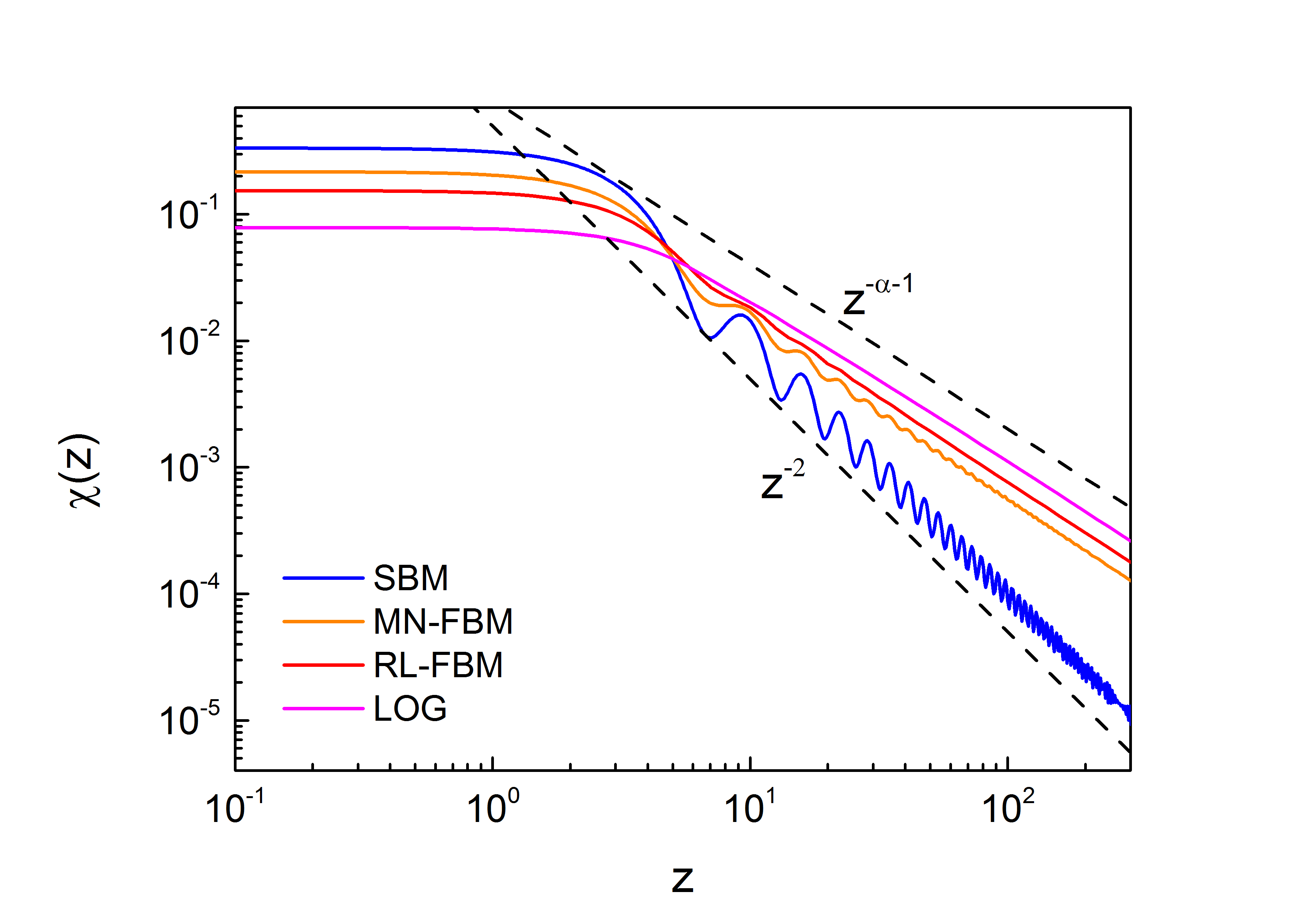
Figure 1: (color online) Frequency scaling function $\chi(z)$ (12) for four models of anomalous diffusion: scaled Brownian motion (SBM), Riemann-Liouville (RL) and Mandelbrot-van Ness (MN) fractional Brownian motion (FBM) and diffusion in a logarithmic potential (LOG) for the scaling exponent $\alpha=0.3$. For identical mean-square displacements in all cases, the asymptotic dependence of $\chi(z)$ for large $z$ (dashed lines) is different, owing to the nonanalytic behavior of the time scaling function $\phi(y)$ for both types of FBM and LOG. The results shown here are exact results obtained by numerical integration of Eq. (12), the asymptotic expansion for large $z$ yields Eqs. (21) through (24).

The time-averaged spectral density in the subdiffusive regime, $0<\alpha<1$, and for long measurement times, $\omega T\gg 1$, is to leading order given by,

$$S_{\text{ta}}^{\text{FBM,LOG}}(\omega) \simeq 2\mathcal{C}a_{\alpha}\Gamma(\alpha+1)\sin\Big{(}\frac{\pi\alpha}{2}\Big{)}\omega^{-\alpha-1}.$$ (22)

Interestingly, even though the process is nonstationary, the spectral density is asymptotically independent of the measurement time, see Fig. 2. This shows that a stationary spectral density does not necessarily imply a stationary process, the nonstationarity being in this case encoded in the low-frequency cutoff. Equation (14) also allows to evaluate finite-time corrections to leading order,

$$S_{\text{ta}}^{\text{FBM,LOG}}(\omega,T) \simeq 2\mathcal{C}\omega^{-\alpha-1}\bigg{[}a_{\alpha}\Gamma(\alpha+1)\sin\Big{(}\frac{\pi\alpha}{2}\Big{)}$$

$$\quad+a_{\alpha}\Gamma(\alpha+1)\cos\Big{(}\frac{\pi\alpha}{2}\Big{)}(\omega T)^{-1}$$

$$\quad+\Big{(}a_{0}-\frac{a_{1}}{\alpha}\Big{)}(\omega T)^{\alpha-1}\bigg{]},$$ (23)

These corrections have two different origins: The dominant terms proportional to $a_{0}$ and $a_{1}$ stem from the nonstationarity of the correlation function. The correction term proportional to $a_{\alpha}$, on the contrary, appears even if the system is perfectly stationary (e.g. for $\alpha<0$) and is due to the finite measurement time.

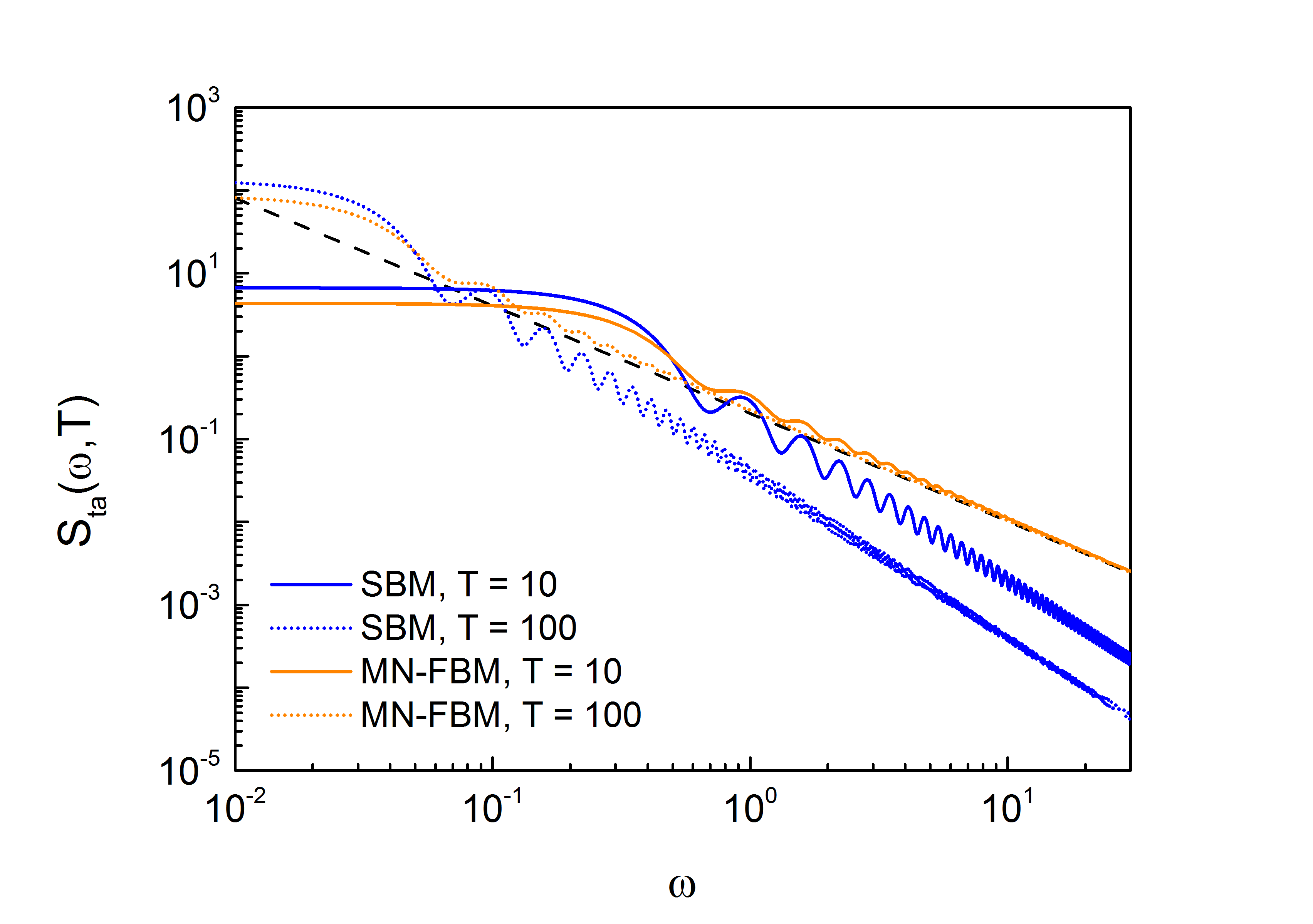
Figure 2: (color online) Time-averaged spectral density $S_{\text{ta}}(\omega,T)$ (12) for scaled Brownian motion (SBM) and Mandelbrot-van Ness fractional Brownian motion (MN-FBM) for $\alpha=0.3$ and different measurement times $T$. The spectral density converges to a stationary expression in the long-time limit for FBM, whereas for SBM, the magnitude of the high-frequency spectrum decreases with time.

In the superdiffusive regime, $1<\alpha<2$, the spectral density of FBM also displays an algebraic time-dependence to leading order,

$$S_{\text{ta}}^{\text{FBM}}(\omega,T) \simeq 2\mathcal{C}\Big{(}a_{0}-\frac{a_{1}}{\alpha}\Big{)}\omega^{-2}T^{\alpha-1}.$$ (24)

The overall magnitude of the spectral density increases with the measurement time $T$. This is similar to the result (21) for superdiffusive SBM.

Relation to $1/f$-noise. As we have seen in Eq. (22), both kinds of FBM and the diffusion in a logarithmic potential lead to a spectral density of the form $S_{\text{ta}}(\omega)\propto\omega^{-\alpha-1}$. Generally, a spectrum with $S(\omega)\propto\omega^{-\beta}$ with $0<\beta<2$ is termed $1/f$-noise dut81 . This kind of spectrum was first observed in flicker noise in triodes joh25 , and has since been found in a wide range of other systems in physics wei88 , biology gil95 , geology dav02 and phonology vos75 . The scaling Wiener-Khinchin relation (12) shows that $1/f$-noise naturally occurs for processes with scale-invariant correlations. The main requirement is that the correlation function is nonanalytic in the limit $t\gg\tau$. Out of the three examples we investigated above, this is the case for FBM and the diffusion in a logarithmic potential, with the former being non-Markovian but linear, and the latter Markovian but nonlinear. For $\alpha<0$, these processes are stationary and the power spectrum, which is proportional to $\omega^{-\alpha-1}$, is integrable at low frequencies, yielding a finite stationary power. For $0<\alpha<1$, by contrast, the stationary spectrum is nonintegrable at low frequencies (infrared catastrophe), formally leading to infinite power. This has caused some discussion on the physical nature of this divergence man67 . Using the scaling Wiener-Khinchin relation (12), this apparent contradiction is easily resolved, since for a diffusive process, the power actually diverges in the infinite time limit. For any finite time, there is a low-frequency cutoff on the spectrum that depends on the measurement time, which ensures finite power. As the measurement time increases, this cutoff moves to lower and lower frequencies, and the process approaches $1/f$-noise at all frequencies. We note that a similar behavior was recently observed for another scale invariant (superdiffusive) stochastic process, the Lévy walk, in application to blinking quantum dots nie13 ; sad14 . Our approach allows to generalize these results to generic subdiffusive random processes.

Conclusion. The generalized Wiener-Khinchin theorem (9)-(10) extends the notion of a power spectrum to nonstationary stochastic processes in a natural way and establishes a direct connection to their autocorrelation functions. By studying three ubiquitous scale-invariant models of anomalous diffusion, we have demonstrated its usefulness in analyzing the properties of aging processes. Our results thus provide an extension of the range of applicability of spectral analysis—in terms of a proper (positive) spectral density—to the nonstationary regime.

Supplemental material

Large argument expansion of $\chi(z)$

In order to obtain the long-time limit of the spectral density, we need to know the asymptotic behavior of the function $\chi(z)$ for large arguments. From Eq. (12) of the main text, $\chi(z)$ is defined as,

$$\chi(z)=\int_{0}^{1}\text{d}v\ v^{\alpha+1}\cos(vz)\int_{\frac{v}{1-v}}^{\infty}\text{d}u\ u^{-\alpha-2}\phi(u)$$ (S25)

We define the auxiliary function,

$$f(v)\equiv v^{\alpha+1}\int_{\frac{v}{1-v}}^{\infty}\text{d}u\ u^{-\alpha-2}\phi(u).$$ (S26)

For the scaling function $\phi(u)$, we assume the asymptotic behavior,

$$\phi(u)\simeq\left\{\begin{array}[]{ll}a_{\lambda}u^{\lambda}&\text{for}\quad u\ll 1\\ b_{\mu}u^{\mu}&\text{for}\quad u\gg 1,\end{array}\right.$$ (S29)

with $\lambda>-1$ and $\mu<\alpha+1$. Using this, it is easy to show that,

$$f(v)\simeq\left\{\begin{array}[]{ll}&a_{\lambda}\Big{[}\frac{1}{\alpha+1-\lambda}v^{\lambda}-v^{\lambda+1}\Big{]}\quad\text{for}\;v\ll 1\\[8.61108pt] &b_{\mu}\Big{[}\frac{1}{\alpha+1-\mu}(1-v)^{\alpha+1-\mu}-\frac{\mu}{\alpha+1-\mu}(1-v)^{\alpha+2-\mu}\Big{]}\quad\text{for}\;1-v\ll 1.\end{array}\right.$$ (S32)

We now split the integral into three parts,

$$\bigg{[}\int_{0}^{\epsilon}+\int_{\epsilon}^{1-\epsilon}+\int_{1-\epsilon}^{1}\bigg{]}\text{d}v\ \cos(vz)f(v),$$ (S33)

where $\epsilon$ is small enough that the expansion (S32) is justified. Using this expansion, we find for large $z$,

$$\int_{0}^{\epsilon}\text{d}v\ \cos(vz)f(v) \simeq a_{\lambda}\Bigg{[}\frac{1}{\alpha+1-\lambda}\bigg{[}-\Gamma(\lambda+1)\sin\Big{(}\frac{\pi\lambda}{2}\Big{)}z^{-\lambda-1}+\frac{\epsilon^{\lambda}\sin(z\epsilon)}{z}+\frac{\lambda\epsilon^{\lambda-1}\cos(z\epsilon)}{z^{2}}\bigg{]}$$

$$\;-\bigg{[}-\Gamma(\lambda+2)\cos\Big{(}\frac{\pi\lambda}{2}\Big{)}z^{-\lambda-2}+\frac{\epsilon^{\lambda+1}\sin(z\epsilon)}{z}+\frac{(\lambda+1)\epsilon^{\lambda}\cos(z\epsilon)}{z^{2}}\bigg{]}\Bigg{]}$$

$$\int_{1-\epsilon}^{1}\text{d}v\ \cos(vz)f(v) \simeq b_{\mu}\Bigg{[}\frac{1}{\alpha+1-\mu}\bigg{[}-\Gamma(\alpha+2-\mu)\cos\Big{(}z-\frac{\pi(\alpha-\mu)}{2}\Big{)}z^{\mu-\alpha-2}-\frac{\epsilon^{\alpha+1-\mu}\sin(z(1-\epsilon))}{z}$$

$$\qquad+\frac{(\alpha+1-\mu)\epsilon^{\alpha-\mu}\cos(z(1-\epsilon))}{z^{2}}\bigg{]}$$

$$\;-\frac{\mu}{\alpha+1-\mu}\bigg{[}\Gamma(\alpha+3-\mu)\sin\Big{(}z-\frac{\pi(\alpha-\mu)}{2}\Big{)}z^{\mu-\alpha-3}-\frac{\epsilon^{\alpha+2-\mu}\sin(z(1-\epsilon))}{z}$$

$$\qquad+\frac{(\alpha+2-\mu)\epsilon^{\alpha-\mu}\cos(z(1-\epsilon))}{z^{2}}\bigg{]}\Bigg{]}$$ (S34)

In the center part of the integral, we may integrate by parts,

$$\int_{\epsilon}^{1-\epsilon} \text{d}v\ \cos(vz)f(v)=\frac{\sin(vz)}{z}f(v)\bigg{|}_{\epsilon}^{1-\epsilon}+\frac{\cos(vz)}{z^{2}}f^{\prime}(v)\bigg{|}_{\epsilon}^{1-\epsilon}+\mathcal{O}(z^{-3}).$$ (S35)

Again using Eq. (S32) for the boundary terms, we see that all terms depending on $\epsilon$ cancel and we are left with,

$$\chi(z) \simeq a_{\lambda}\bigg{[}-\frac{\Gamma(\lambda+1)}{\alpha+1-\lambda}\sin\Big{(}\frac{\pi\lambda}{2}\Big{)}z^{-\lambda-1}+\Gamma(\lambda+2)\cos\Big{(}\frac{\pi\lambda}{2}\Big{)}z^{-\lambda-2}\bigg{]}$$

$$\quad+\frac{b_{\mu}}{\alpha+1-\mu}\bigg{[}-\Gamma(\alpha+2-\mu)\cos\Big{(}z-\frac{\pi(\alpha-\mu)}{2}\Big{)}z^{\mu-\alpha-2}-\mu\Gamma(\alpha+3-\mu)\sin\Big{(}z-\frac{\pi(\alpha-\mu)}{2}\Big{)}z^{\mu-\alpha-3}.$$ (S36)

For $\mu<\alpha-\lambda$, which is the case for all the examples discussed in the main text, the leading order expression is given by the part proportional to $a_{\lambda}$, which is precisely Eq. (14) of the main text.

Asymptotic expressions for $\phi(u)$ for the example systems

	$\{\lambda_{i}\}$	$\{a_{\lambda_{i}}\}$	$\{\mu_{i}\}$	$\{b_{\mu_{i}}\}$
SBM	$0$	$1$	$0$	$1$
RL-FBM	$0;\ \alpha;\ 1;\ \ldots$	$1;\ -\frac{\sqrt{\pi}\Gamma((\alpha+1)/2)}{\Gamma(\alpha/2)\sin(\pi\alpha/2)};\ \frac{\alpha}{2};\ \ldots$	$\frac{\alpha-1}{2};\ \frac{\alpha-3}{2};\ \frac{\alpha-5}{2};\ \ldots$	$\frac{2\alpha}{\alpha+1};\ \frac{\alpha(\alpha-1)}{\alpha+3};\ \frac{\alpha(\alpha-1)(\alpha-3)}{4(\alpha+5)};\ \ldots$
MN-FBM	$0;\ \alpha;\ 1;\ \ldots$	$1;\ -1;\ \frac{\alpha}{2};\ \ldots$	$0;\ \alpha-1;\ \alpha-2;\ \ldots$	$\frac{1}{2};\ \frac{\alpha}{2};\ \frac{\alpha(\alpha-1)}{4};\ \ldots$
LOG	$0;\ \alpha;\ \ldots$	$\frac{\sqrt{\pi}}{2\Gamma(3-\alpha)};\ -\frac{\pi\Gamma(2-\alpha)\Gamma(1-\alpha)}{4\Gamma^{2}(3/2-\alpha)};\ \ldots$	$\alpha-\frac{3}{2};\ \alpha-\frac{5}{2};\ \ldots$	$\frac{\sqrt{\pi}\alpha\Gamma(7/2-\alpha)}{3\Gamma(3-\alpha)};\ \frac{\sqrt{\pi}\alpha(3-2\alpha)\Gamma(9/2-\alpha)}{10(\alpha-3)\Gamma(3-\alpha)};\ \ldots$

In the main text, we discuss the spectral density for scaled Brownian motion (SBM), Riemann-Liouville (RL-FBM) and Mandelbrot-van Ness (MN-FBM) fractional Brownian motion and diffusion in a logarithmic potential (LOG). The table lists the explicit expressions for the coefficients and exponents of the small argument ($\phi(u)\simeq a_{\lambda_{1}}u^{\lambda_{1}}+a_{\lambda_{2}}u^{\lambda_{2}}+\ldots$) and large argument ($\phi(u)\simeq b_{\mu_{1}}u^{\mu_{1}}+b_{\mu_{2}}u^{\mu_{2}}+\ldots$) expansions of the corresponding scaling functions. The first column lists the stochastic model, the second column the first few exponents $\lambda_{i}$ in the small-argument expansion in ascending order (for $0<\alpha<1$). The third column lists the coefficients corresponding to these exponents. The fourth and fifth column are the same, but for the large-argument expansion. So, for example, the first three terms in the small argument expansion for the scaling function for MN-FBM motion are,

$$\phi(u)\simeq 1-u^{\alpha}+\frac{\alpha}{2}u+\mathcal{O}(u^{2}).$$ (S37)

Note that each of the exponents $\lambda_{i}$ and $\mu_{i}$ individually yields a contribution of the type (S8) to the expansion of the frequency scaling function $\chi(z)$.

References

- (1) N. Wiener, Acta Math. 55, 117 (1930).
- (2) A. Khinchin, Math. Annalen 109, 604 (1934).
- (3) R. Ziemer and W. H. Tranter, Principles of Communications: Systems, Modulation and Noise (Wiley, New York, 2014).
- (4) R. D. Yates and D. J. Goodman, Probability and Stochastic Processes: A Friendly Introduction for Electrical and Computer Engineers, (Wiley, New York, 2004).
- (5) H. Risken, The Fokker-Planck Equation (Springer, Berlin, 1989).
- (6) J. W. Goodman, Statistical Optics (Wiley, New York, 1985).
- (7) L. Mandel and E. Wolf, Optical Coherence and Quantum Optics (Cambridge, Cambridge, 1995).
- (8) L. Cohen, Time-Frequency Analysis (Prentice-Hall, Upper Saddle River, 1995).
- (9) E. P. Wigner, Phys. Rev. 40, 749 (1932).
- (10) J. Ville, Cables et Trans., 2, 61 (1948).
- (11) J. P. Bouchaud and A. Georges, Phys. Rep. 195, 127 (1990).
- (12) D. ben-Avraham and S. Havlin, Diffusion and Reactions in Fractals and Disordered Systems, (Cambridge, Cambridge, 2000).
- (13) J. B. Bassingthwaighte, L. S. Liebovitch and B. J. West, Fractal Physiology, (Oxford, Oxford, 1994).
- (14) B. B. Mandelbrot, Fractals and Scaling in Finance, (Springer, Berlin, 1997).
- (15) D. Brockmann L. Hufnagel and T. Geisel, Nature 439, 462 (2006).
- (16) R. Metzler and J. Klafter, Phys. Rep. 339, 1 (2000).
- (17) P. Dutta and P. M. Horn, Rev. Mod. Phys. 53, 497 (1981).
- (18) W. Martin and P. Flandrin, IEEE T. Acoust. Speech 33, 1461 (1985).
- (19) A. Dechant, E. Lutz, D. A. Kessler and E. Barkai, Phys. Rev. X 4, 011022 (2014).
- (20) A. Papoulis, Probability, Random Variables and Stochastic Processes, (McGraw-Hill, New York, 1991).
- (21) See Supplementary Material, which contains the asymptotic expansion of the frequency scaling function and explicit expressions for the coefficients in the expansion of the time scaling function.
- (22) S. C. Lim and S. V. Muniandy, Phys. Rev. E 66, 021114 (2002).
- (23) F. Thiel and I. M. Sokolov, Phys. Rev. E 89, 012115 (2014).
- (24) P. Lévy, Random Functions: General Theory with Special References to Laplacian Random Functions, (University of California Press, Berkeley, 1953).
- (25) B. B. Mandelbrot and J.W. Van Ness, SIAM Rev. 10, 422 (1968).
- (26) I. Golding and E. C. Cox, Phys. Rev. Lett. 96, 098102 (2006).
- (27) S. C. Weber, A. J. Spakowitz, and J. A. Theriot, Phys. Rev. Lett. 104, 238102 (2010).
- (28) J.-H. Jeon, V. Tejedor, S. Burov, E. Barkai, C. Selhuber-Unkel, K. Berg-Sorensen, L. Oddershede, and R. Metzler, Phys. Rev. Lett. 106, 048103 (2011).
- (29) S. M. A. Tabei, S. Burov, H. Y. Kim, A. Kuznetsov, T. Huynh, J. Jureller, L. H. Philipson, A. R. Dinner, and N. F. Scherer, Proc. Natl. Acad. Sci. USA 110, 4911 (2013).
- (30) A. Dechant, E. Lutz, D. A. Kessler and E. Barkai, Phys. Rev. Lett. 107, 240603 (2011).
- (31) A. Dechant, E. Lutz, D. A. Kessler and E. Barkai, Phys. Rev. E 85, 051124 (2012).
- (32) E. Lutz and F. Renzoni, Nature Phys. 9, 615 (2013).
- (33) F. Bouchet and T. Dauxois, Phys. Rev. E 72, 045103(R) (2005).
- (34) H. C. Fogedby and R. Metzler, Phys. Rev. Lett. 98, 070601 (2007).
- (35) E. Lutz, Phys. Rev. A 67, 051402 (2003).
- (36) J. B. Johnson, Phys. Rev. 26, 71 (1925).
- (37) M. B. Weissmann, Rev. Mod. Phys. 60, 537 (1988).
- (38) D. L. Gilden, T. Thornton, M. W. Mallon, Science 267, 1837 (1995).
- (39) J. Davidsen and H. G. Schuster, Phys. Rev. E 65, 026120 (2002).
- (40) R. F. Voss and J. Clarke, Nature 258, 317 (1975).
- (41) B. B. Mandelbrot, IEEE T. Inform. Theory 13, 293 (1967).
- (42) M. Niemann, H. Kantz, and E. Barkai, Phys. Rev. Lett. 110, 140603 (2013).
- (43) S. Sadegh, E. Barkai and D. Krapf, New J. Phys. 16, 113054 (2014).