New Insights into Time Series Analysis

Abstract

Context. The first step when investigating time varying data is the detection of any reliable changes in star brightness. This step is crucial to decreasing the processing time by reducing the number of sources processed in later, slower steps. Variability indices and their combinations have been used to identify variability patterns and to select non-stochastic variations, but the separation of true variables is hindered because of wavelength-correlated systematics of instrumental and atmospheric origin, or due to possible data reduction anomalies.

Aims. The main aim is to review the current inventory of correlation variability indices and measure the efficiency for selecting non-stochastic variations in photometric data.

Methods. We test new and standard data-mining methods for correlated data using public time-domain data from the WFCAM Science Archive (WSA). This archive contains multi-wavelength calibration data (WFCAMCAL) for $\rm 216,722$ point sources, with at least 10 unflagged epochs in any of five filters (YZJHK), which were used to test the different indices against. We improve the panchromatic variability indices and introduce a new set of variability indices for preselecting variable star candidates. Using the WFCAMCAL Variable Star Catalogue (WVSC1) we delimit the efficiency of each variability index. Moreover we test new insights about these indices to improve the efficiency of detection of time-series data dominated by correlated variations.

Results. We propose five new variability indices which display a high efficiency for the detection of variable stars. We determine the best way to select variable stars using these and the current tool inventory. In addition, we propose an universal analytical expression to select likely variables using the fraction-of-fluctuations on these indices ($f_{\rm fluc}$). The $f_{\rm fluc}$ can be used as an universal way to analyse photometric data since it displays a only weak dependency with the instrument properties. The variability indices computed in this new approach allow us to reduce misclassification and these will be implemented in an automatic classifier which will be addressed in a forthcoming paper in this series.

Conclusions.

1 Introduction

The tremendous development in astronomical instrumentation and automation during the last few decades has given rise to several questions about how to analyse and synthesize the growing amount of data. Recently, various dedicated telescope systems, both on the ground and in space, have been used for wide-field shallow, low resolution, multi-epoch, imaging surveys, scanning the sky in different wavebands with aims ranging from comprehensive stellar variability searches to exoplanet hunting e.g. (PanSTARRS, Kaiser et al. (2002);OGLE, Udalski (2003); SUPERWASP, Pollacco et al. (2006); CoRoT, Baglin et al. (2007); NSVS, Hoffman et al. (2009); Kepler, Borucki et al. (2010)). These data have led to many discoveries in several areas of modern astronomy: asteroseismology, exoplanets and stellar evolution (e.g., Huber et al., 2012; De Medeiros et al., 2013; Walkowicz & Basri, 2013; Paz-Chinchón et al., 2015). The next generation of these surveys, such as Gaia (Bailer-Jones et al., 2013) and the VISTA Variables in Vía Láctea survey (VVV; Minniti et al. 2010), are providing a high data flow for a wide range of science applications in order to understand the dynamics and stellar variability of the Milky Way galaxy.

The first step to investigating time varying data is the detection of any reliable changes in star brightness (e.g. Welch & Stetson, 1993; Stetson, 1996; Wozniak, 2000; Shin et al., 2009; Ferreira Lopes et al., 2015). This step is crucial to decreasing the running time by reducing the number of sources that slower steps, such as period finding and classification, are run on. The stochastic variations are mainly related to very bright sources, caused by saturation of the detector whereby the flux within the aperture will bleed out into nearby pixels and the measured magnitude becomes dependent on the sky brightness and seeing, or very faint sources where the sky noise dominates, providing an increase in the uncertainty of the measurements, and a dependency on the sky brightness and seeing. Variability indices and their combinations have been used to identify variability patterns and to select non-stochastic variations (e.g. Damerdji et al., 2007; Shin et al., 2009; Ferreira Lopes et al., 2015), but the separation of true variables from noisy data is hindered because of wavelength-correlated systematics of instrumental and atmospheric origin, or due to possible data reduction anomalies. Detection methods have been optimized for specific variability signals to detect supernovae, microlensing, transits, and other variable sources (e.g. Alard & Lupton, 1998; Wozniak, 2000; Gössl & Riffeser, 2002; Becker et al., 2004; Corwin et al., 2006; Yuan & Akerlof, 2008; Renner et al., 2008). An important step to optimising this process is to review the current inventory of variability indices and determine the efficiency level for selecting non-stochastic variations in photometric data.

Table 1: Variability Indices analyses in the present work. The description of terms used in this indices are discriminate in Sect. 3.1 and 3.2.

Index	Definition	Reference
$I_{WS}$	$\sqrt{\frac{1}{n\cdot(n-1)}}\sum_{n=1}^{N-1}\left(\frac{x_{n}-\mu}{e_{n}}\right)\cdot\left(\frac{x_{n+1}-\mu}{e_{n+1}}\right)$	Welch & Stetson 1993
$J_{WS}$	$\sum_{n=1}^{N-1}sign(\delta_{n}\delta_{n+1})\sqrt{\left|\delta_{n}\delta_{n+1}\right|}$	Stetson 1996
$K_{WS}$	$\frac{1/N\sum_{i=1}^{N}\left|\delta_{i}\right|}{\sqrt{1/N\sum_{i=1}^{N}\delta_{i}^{2}}}$	Stetson 1996
$L_{WS}$	$\left(J_{WS}\cdot K_{WS}\right)/0.789$	Stetson 1996
$I_{\rm pfc}^{(s)^{\prime}}$	$\!\frac{1}{n_{s}}\sum_{i=1}^{n}\left[\sum_{j_{1}=1}^{m-(s-1)}\!\!\!\cdots\left(\sum_{j_{s}=j_{(s-1)}+1}^{m}\!\!\!\Lambda_{ij_{1}\cdots j_{s}}^{(s)}\sqrt[s]{\left|\Gamma u_{ij_{1}}\cdots\Gamma u_{ij_{s}}\right|}\right)\right]$	Ferreira Lopes et al. 20151
$I_{\rm fi}^{(s)}$	$0.5\cdot\left\{1+\frac{1}{n_{s}}\sum_{i=1}^{n}\left[\sum_{j_{1}=1}^{m-(s-1)}\cdots\left(\sum_{j_{s}=j_{(s-1)+1}}^{m}\Lambda_{ij_{1}\cdots j_{s}}^{(s)}\right)\right]\right\}$	Ferreira Lopes et al. 2015
$K_{fi}^{(s)}$	$\frac{N_{s}^{+}}{N_{s}}$	the present work
$L_{pfc}^{(s)}$	$\frac{1}{N_{s}}\sum_{k=1}^{N_{box}}Q_{(s,k)}$	the present work
$M_{pfc}^{(s)}$	$med[Q_{(s)}]$	the present work
$FL^{(s)}$	$F^{(s)}\times L_{pfc}^{(s)}$	the present work
$FM^{(s)}$	$F^{(s)}\times M_{pfc}^{(s)}$	the present work

1. Unfortunately the first version of $I_{pfc}^{(s)^{\prime}}$ indices was incorrectly defined. Therefore, the authors have since added an erratum with the correct form..

The second step is to determine the main periods. There are various methods used in astronomy for frequency analysis, to name a few: the Deeming method (Deeming, 1975), PDM-Jurkevich (Stellingwerf, 1978; Dupuy & Hoffman, 1985), string length minimization (Lafler & Kinman, 1965; Stetson, 1996; Clarke, 2002), information entropy (Cincotta et al., 1995), the analysis of variance (ANOVA, Schwarzenberg-Czerny, 1996) and the Lomb-Scargle and its extension using error bars (Lomb, 1976; Scargle, 1982; Zechmeister & Kürster, 2009). These methods are based on the fact that the phase diagram of the light curves (LCs) is smoothest when it is visualized using its real frequencies. Assessment of the significance of these frequencies is a pertinent problem due to non-Gaussianity, multi-periodicity, non-periodic variations, and the manner of how they should be taken into account (Süveges, 2014). From this view the variability indices are a fundamental part of the variability analysis in order to save running time and decrease the number of miscalculations in the frequency analysis. The detection of non-periodic variables, transients, and other aspects in regard to the significance of peaks in a periodogram has not been completely solved yet.

The last point is that the variability classification is intrinsically related with the determination of reliable periods and determining a set of parameters that allows us to distinguish all variability types. Automatic classifiers based on machine learning have been applied to several large time-series datasets (e.g. Woźniak et al., 2004; Debosscher et al., 2007; Sarro et al., 2009; Blomme et al., 2010; Richards et al., 2011; Dubath et al., 2012). The inclusion of periodic and non-periodic features, statistics and more sophisticated model parameters have improved automatic classifiers (e.g. Richards et al., 2011). Misclassification, fuzzy boundaries between variable stars’ classes, mis-labelled training sets, as well as, full processing of terabytes of data are current scientific challenges (Eyer, 2006).

The present paper is the first in a series of papers covering different aspects of variable star selection and classification. The first two articles are related to selection of variable stars using variability indices. In this paper, we discuss the selection of variable stars using correlation variability indices, while in the second of this series we will discuss non-correlation variability indices; Paper 3 will be about periodicity search methods; Paper 4 will be about the variable star classifier. In this work, we perform a comprehensive stellar variability analysis on time varying data. In Sect. 2.1, we describe the data used to compare each index, using a pre-selected catalogue of known variable stars to test how well each index selects these and the efficiency of the selection measured by how few additional stars are selected by the same cutoff value. In Sect. 3, we present an overview of commonly used correlation variability indices and propose 5 new variability indices. Next, in Sect. 4 we analyse the limits of correlated variability indices as well as proposing a false alarm probability for variability indices. We present our results and discussions in Sect. 6. Finally, in Sect. 7, we draw our conclusions and discuss some future perspectives.

2 Data

2.1 WFCAMCAL database

The public WFCAM Calibration (WFCAMCAL - Hodgkin et al., 2009; Cross et al., 2009) is an unique programme that is well fitted to test the panchromatic variability indices and our assumptions. This programme contains panchromatic data for 58 different pointings distributed over the full range in right ascension and spread over declinations of $+59\aas@@fstack{\circ}62$ and $-24\aas@@fstack{\circ}73$. These were used to calibrate the UKIDSS surveys Lawrence et al. 2007. The pointing closest to the zenith was chosen whenever a calibration field was observed. This was typically every hour early on in the UKIDSS observations and later every 2 hours, with some early nights having many additional observations (up to 40 in a night). During each visit the fields were usually observed with a sequence of filters, either through $JHK$ or $ZYJHK$ filters within a few minutes. This lead to an irregular sampling with fields observed again roughly on a daily basis, although longer time gaps are common, and of course large seasonal gaps are also present in the data set.

The WFCAMCAL data are archived in the WFCAM Science Archive (WSA; Hambly et al. 2008). The data are processed by the Cambridge Astronomy Survey Unit (CASU) Irwin et al. (2004) and the Wide Field Astronomy Unit (WFAU) in Edinburgh, and the latter produce the WSA. The design of the WSA, the details of the data curation procedures and the layout of the database are described in detail in Hambly et al. 2008 and Cross et al. 2009. We use data from the WFCAMCAL08B release (observations upto the end of UKIRT semester 08B).

2.2 The WFCAMCAL Variable Star Catalogue

Ferreira Lopes et al. 2015 performed a comprehensive stellar variability analysis of the WFCAMCAL database and presented the photometric data and characteristics of the identified variable stars as the WFCAM Variable Star Catalogue (WVSC1). The authors used standard data-mining methods and introduced new variability indices designed for multiband data with correlated sampling. To summarize, the authors performed a careful analysis using cutoff surfaces to obtain a preselection with $6651$ stars based on criteria established by numerical tests of the noise characteristics of the data. Next they combined four frequency analysis methods to search for the real frequencies in the LCs in each waveband and in the chromatic LC, i.e. comprised of the sum of all broadband filters. Finally, they obtained a ranked list of the best periods for each method and selected the very best period, which gave the minimum $\chi^{2}$ in order to cope with aliasing. Finally, the authors visually inspected all the phase diagrams of the $6651$ stars and recovered a catalogue containing $319$ stars in which $275$ are classified as periodic variable stars and $44$ objects as suspected variables or apparently aperiodic variables.

In this paper we analyse this same sample from Ferreira Lopes et al. 2015. First, we selected all sources classified as a star or probable star having at least ten unflagged epochs in any of the five filters. This selection was performed from an initial database of $216,722$ stars. Next we test the efficiency of selection of variable stars using the variability indices presented in Sect. 3.

3 Variability Indices

Table 1 summarises 12 variability indices of which 5 are new indices proposed in this work. The present work discusses the efficiency of selection of each one and discusses the best way to select variable stars using the current tool inventory. Sets of variability indices have been used, instead of one, to improve the selection process during the last few years (e.g. Shin et al., 2009). Indeed automatic classifiers are also using these parameters to facilitate the classification of variable stars (e.g. Richards et al., 2011). The variability indices are a fundamental tool to improving all processes of the time domain analysis.

Currently, the Welch-Setson indices (e.g. Welch & Stetson, 1993; Stetson, 1996, i.e. $I_{WS}$, $J_{WS}$, $K_{WS}$ and $L_{WS}$ indices) are found to be significantly more sensitive than the “traditional” $\chi^{2}$-test for single variance, which uses the magnitude-rms scatter distribution of the data as a predictor (e.g. Pojmanski, 2002). The improvements proposed by Stetson 1996 on $I_{WS}$ (Welch & Stetson, 1993) and incorporated in the $J_{WS}$ index allow us to compare wavebands with different numbers of epochs on an equal basis. The author uses the Bessel correction ($\sqrt{\frac{n}{n-1}}$) to reduce the bias related with the sample size despite the index being the square of the correlation not the mean variance. The $I_{WS}$ index was modified, to quantify panchromatic flux correlations, to form new variability indices ($I_{\rm pfc}^{(s)^{\prime}}$) by Ferreira Lopes et al. 2015. These were the first variability indices developed to analyse panchromatic surveys. Moreover the authors proposed a new set of flux independent variability indices ($I_{\rm fi}^{(s)}$).

The statistical period search based in the analysis of variance (ANOVA, Schwarzenberg-Czerny, 1996) has been used to select non-stochastic variations. Nevertheless, this method is limited to identification of periodic variations and requires more running time once its significance level is determined on phase diagrams for each frequency test. Using variability indices we can discriminate non-stochastic variations independently from their nature and reduce the running time. The main goal of this work is to determine the best way to select variable stars without computing the variability periods. In the follow subsection we summarize the $I_{\rm pfc}^{(s)^{\prime}}$ and $I_{\rm fi}^{(s)}$ variability indices as well as improvements on these indices using a new approach.

3.1 The $I_{\rm pfc}^{(s)^{\prime}}$ and $I_{\rm fi}^{(s)}$ panchromatic variability indices

The current tool inventory was added to by Ferreira Lopes et al. 2015 with a new set of variability indices to separate LCs that are dominated by correlated variations from those that are noise-dominated ones. The authors introduced a new set of variability indices designed for multi-band data with correlated sampling that included one index that is highly insensitive to the presence of outliers in the time-series data. First, the authors extended $I_{\rm WS}$ to create the $I_{pfc}$ index defined as,

$$I_{\rm pfc}^{(s)^{\prime}}=\!\frac{1}{n_{s}}\sum_{i=1}^{n}\left[\sum_{j_{1}=1}^{m-(s-1)}\!\!\!\cdots\left(\sum_{j_{s}=j_{(s-1)}+1}^{m}\!\!\!\Lambda_{ij_{1}\cdots j_{s}}^{(s)}\sqrt[s]{\left|\Gamma u_{ij_{1}}\cdots\Gamma u_{ij_{s}}\right|}\right)\right],$$ (1)

where $m$ is the number of filters, $s$ is the combination type (between two or more epochs), $n_{s}$ is the total number of correlations, and the $\Lambda^{(s)}$ correction factor is,

$$\Lambda_{ij_{1}\cdots j_{s}}^{(s)}=\left\{\begin{array}[]{ll}+1&\qquad\mbox{if \,\, $\Gamma u_{ij_{1}}>0,\,\,\cdots\,,\,\Gamma u_{ij_{s}}>0$ };\\ +1&\qquad\mbox{if \,\, $\Gamma u_{ij_{1}}<0,\,\,\cdots\,,\,\Gamma u_{ij_{s}}<0$ };\\ -1&\qquad\mbox{otherwise}.\end{array}\right.$$ (2)

and $\Gamma$ is given by,

$$\Gamma u_{ij}=\sqrt{\frac{n_{u_{j_{s}}}}{n_{u_{j_{s}}}-1}}\times\left(\frac{u_{ij_{s}}-\bar{u}_{j_{s}}}{\sigma_{u_{ij_{s}}}}\right).$$ (3)

These indices allow us to compute correlations among $s$ epochs. As shown by the authors, increasing the number of correlated wave bands (s) makes the separation between correlated and uncorrelated variables more evident. Next the authors proposed a new index, $I_{fi}^{(s)}$, using Eqn 2 that is the sum of discrete values 1 or -1. This index is defined as

$$2\cdot I_{\rm fi}^{(s)}-1=\frac{1}{N_{s}}\sum_{i=1}^{n}\left[\sum_{j_{1}=1}^{m-(s-1)}\cdots\left(\sum_{j_{s}=j_{(s-1)+1}}^{m}\Lambda_{ij_{1}\cdots j_{s}}^{(s)}\right)\right]\,,$$ (4)

where $0\leq I_{\rm fi}^{(s)}\leq 1$, and where $\Lambda_{ij_{1}\cdots j_{s}}^{(s)}$ is defined in Eqn (2). Finally the authors propose a general expression to determine the probability of a random event leading to a positive $I_{\rm fi}^{(s)}$ index. In the case of statistically independent events, this is given by,

$$P_{s}=\frac{2}{s^{2}}.$$ (5)

On the other hand the expected value of $I_{\rm pfc}^{(s)^{\prime}}$ for a random distribution is about $0$. Meanwhile, the number of sources with negative values increase with $s$, because there is an increase in the number of possible combinations that give a negative correlation.

3.2 Improvements on panchromatic and flux independent indices

The $I_{\rm pfc}^{(s)^{\prime}}$ variability indices (see Eqn. 1) would work equally well if a set of observations are in the same bandpass, if we correlated groups of observations observed over a short interval. Therefore we need to modify the $I_{\rm pfc}^{(s)^{\prime}}$ indices to make them still more robust against different numbers of observations in each group. Similarly, we propose a new panchromatic, flux independent, variability index ($K_{\rm fi}^{(s)}$) and additionally combine these indices to create two new indices. In order to provide an expression to be used in multi or single waveband data we propose the follow notation:

1. First, we compute the values of $\delta_{i}$ give by

   $$\delta_{i}=\sqrt{\frac{n_{x}}{n_{x}-1}}\cdot\left(\frac{x_{i}-\bar{x}}{\sigma_{x,i}}\right).$$ (6)

   where $n_{x}$ is the number of epochs of waveband $x$, $x_{i}$ are the flux measurements, $\bar{x}$ is the mean flux and $\sigma_{x,i}$ denotes the flux errors. This parameter is equal to that used by Stetson 1996 to improve $I_{WS}$ index and according to him the measurements of correlations using $\delta_{i}$ allow us to compare data from different wavebands with unequal numbers of observations on an equal basis.

2. Next, the $\delta_{i}$ values are computed for all measurements in each waveband using the respective values of $n_{x}$. As a result we obtain a vector $\delta$ with $N$ measurements collected in any waveband. In addition, we save the observation time for each $\delta_{i}$ value.

3. We determine the time interval ($\Delta T$) for which measurements enclosed in this interval will be considered to be at virtually the same epoch. The chosen $\Delta T$ value comes from the arrangement of epochs and thus gives the minimum period (see Sect. 4.3). The total number of boxes ($N_{box}$) is given by $T_{tot}/\Delta T$, where $T_{tot}$ is the total time spam. The accuracy of the index must increase as $\Delta T$ decreases.

4. Next we compute the value of the variability index of order $s$ in the $k^{th}$ box;

   $$Q_{(s,k)}=\left\{\begin{array}[]{ll}\sum_{j_{1}=1}^{n_{k}-(s-1)}\!\!\!\cdots\sum_{j_{s}=j_{(s-1)}+1}^{n_{k}}\left(\Lambda_{j_{1},\!\!\!\cdots,j_{s}}\!\!\!\cdot\sqrt[s]{\left|\delta_{j_{1}}\!\!\!\cdots\delta_{j_{s}}\right|}\right)&\quad\mbox{if $j_{1}\neq j_{s}$};\\ 0&\quad\mbox{if $n_{k}\leq 1$.}\end{array}\right.$$ (7)

   This equation performs all possible combinations without repetition among the $n_{k}$ values. Indeed the total number of combinations calculated is given by,

   $$N_{s}=\sum_{k=1}^{N_{box}}\frac{n_{k}!}{[s!(n_{k}-s)!]}.$$ (8)

5. Now, we can express the flux independent indices on a simple expression given by,

   $$K_{\rm fi}^{(s)}=\frac{N_{s}^{+}}{N_{s}}$$ (9)

   where $N_{s}^{+}$ are the number of positive correlations according to Eqn. 2. $K_{\rm fi}^{(s)}$ indices include measurements obtained in one filter in contrast to $I_{\rm fi}^{(s)}$ indices where measurements are obtained in different filters.

6. Next, we can compute the $L_{\rm pfc}^{(s)}$ index given by,

   $$L_{pfc}^{(s)}=\frac{1}{N_{s}}\sum_{k=1}^{N_{box}}Q_{(s,k)}.$$ (10)

   where it reduces to $J_{pfc}^{(s)}$ in the case when we only have measurements in different filters. $L_{pfc}^{(s)}$ can be used to perform comparisons on an equal basis between stars with different number of epochs as well as using measurements obtained in one filter in contrast to $J_{\rm pfc}^{(s)}$ and $K_{\rm fi}^{(s)}$ indices.

7. An alternative way to compute the characteristic value of correlation is computing the median of correlations, given by

   $$M_{pfc}^{(s)}=med\left[Q_{(s)}\right],$$ (11)

   where $Q_{(s)}$ encloses all $Q_{(s,k)}$ correlations. The median value may provide a more robust value than the mean in the presence of outliers.

8. Finally, we can use the $K_{\rm fi}^{(s)}$ in a correction factor related to instrument properties and outliers. Such a factor can be defined as,

   $$F^{(s)}=\left\{\begin{array}[]{ll}2\cdot\left(K_{\rm fi}^{(s)}-P_{s}\right)&\quad\mbox{if $K_{\rm fi}^{(s)}\geq P_{s}$};\\ 0&\quad\mbox{otherwise}\end{array}\right.$$ (12)

   where $P_{s}$ is the expected value of pure noise for $K_{\rm fi}^{(s)}$. $F^{(s)}$ ranges from $0$ to $2\times(1-2/s^{2})$ providing an increase of its weight with s values. For instance, the maximum value of $F^{(s)}$ is $1$ for $s=2$ and $\sim 1.6$ for $s=3$. $F^{(s)}$ is more efficient than $K_{\rm fi}^{(s)}$ because this increases the difference between values of correlated and uncorrelated data and we concentrate the pure noise values about zero. $F^{(s)}$ is used for provide a new set of indices given by $FL^{(s)}$ and $FM^{(s)}$ (see Table 1).

The variability indices proposed above are determined using properties related with the magnitude and signal correlation values. Stellar variability searches based on such indices follow general assumptions: (i) intrinsic stellar variability can be typically identifiable from analysis of correlation measures observed in multiple or single wavebands; (ii) there are a minimum number of correlations required to discriminate stochastic and non-stochastic variations (see Sect. 4.1); (iii) the interval between any 2 observations ($\tau$) used to compute the correlations must be sufficiently phase-locked (see Sect. 4.3); (iv) non-intrinsic variations will be typically stochastic. Indeed measurements due the systematics of instrumental and atmospheric origin, or due to possible data reduction anomalies, displaying correlated properties may decrease the confidence level of variability indices. Such measurements are mainly related with temporal saturation of bright objects as well as systematic variations in the sky noise for faint stars.

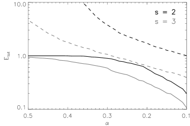
Figure 1: Efficiency metric ($E_{tot}$: the ratio of total number of sources in the selection to good known variables in WVSC1) using Eqn. 16 for $s=2$ (black lines) and for $s=3$ (grey lines). Solid lines mark $E_{WVSC1}$, the fraction of the good variables in the selection, while the dashed lines mark $E_{tot}$. A good choice of $\alpha$ returns a high fraction of good variables $E_{WVSC1}$ for a low value of the efficiency metric $E_{tot}$.

4 Detection limits of correlated variability indices

The number of measurements and how many measurements are ‘close’ - i.e. within a time span much shorter than the period of any variability - are fundamental information necessary to set better variability indices. The number of measurements will determine how stringent the cutoff values must be while the number of close measurements will set the most appropriate variability index. To determine which measurements are close or not we need to determine a $\Delta T$ value such that it is a compromise between the number of correlated measurements and the minimum period that we are searching for. For instance, variability indices computed in boxes of $\Delta T$, greater than the period, will return values closer to those expected for noise. Lower values of $\Delta T$ lead to higher accuracy for variability indices that use correlation measurements.

Moreover, variability indices can be used in all processes of the time-series analysis such as discussed in previous sections. Therefore we must find new ways that allow us to increase the precision, reliability of these indices and their connexions with the different types of variability. In Sect. 3 we described the current tool inventory and we proposed new variability indices with new correction factors to reduce bias. In the present section we propose new ways to increase the precision of these variability indices as well as how to evaluate their reliability.

4.1 Number of correlated measurements

The minimum number of measurements that are enough for the use of a variability index will be determined by the capability of separating variable and non-variable stars. The statistical properties like mean, standard deviation, skewness and kurtosis will be strongly dependent on the number of measurements. On the other hand, we need contemporary (close) measurements to use correlated variability indices. These features may change for each variability index.

Consider two cases: one with $N_{s}$ correlated data points and the other with $N_{s}$ of pure noise for $s=2$. In the case of pure noise, the number of positive and negative correlation must be the same $(N_{s}^{+}=N_{2}/2)$, while for correlated data $(N_{s}^{+}=N_{2})$. Using $K_{\rm fi}^{(s)}$ indices we can determine the minimum number of correlations necessary to separate a purely correlated signal from pure noise assuming that there is an uncertainty in the sign of some correlations. We assume that this uncertainty (or fluctuation) on the number of positive correlations given by $n_{f}$ provides an increase in the variability index of pure noise and a decrease otherwise. So the minimum separation between correlated and uncorrelated data is given by,

$$\Delta K_{\rm fi}^{(2)}=\left(\frac{N_{2}-n_{f}}{N_{2}}\right)-\left(\frac{\frac{N_{2}}{2}+n_{f}}{N_{2}}\right)>0\quad\Rightarrow\quad N_{2}^{min}=4\cdot n_{f}$$ (13)

where $n_{f}$ is an integer with values less than $N_{2}/2$. The minimum number of correlations must be at least 5 according to this relation, given a single error. The general expression is given by,

$$\Delta K_{\rm fi}^{(s)}=\left(\frac{N_{s}-n_{f}}{N_{s}}\right)-\left(\frac{P_{s}N_{s}+n_{f}}{N_{s}}\right)>0\quad\Rightarrow\quad N_{s}^{min}=\frac{2n_{f}}{1-P_{s}},$$ (14)

where the minimum value ($\Delta K_{\rm fi}^{(s)}$) to validate this relation is given by,

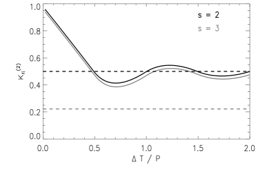
Figure 2: $K_{fi}^{(s)}$ versus $\Delta T/P$ for $s=2$ (black lines) and for $s=3$ (grey lines). The dashed lines mark the expected values for random variation.

$$\Delta K_{\rm fi}^{(s)}=1-P_{s}-\frac{2n_{f}}{N_{s}}.$$ (15)

where $n_{f}/N_{s}$ is the fractional fluctuation of positive correlated measures ($f_{\rm fluc}$). This equation explains analytically the increase in precision as well as the detachment between correlated and non-correlated data with increasing $s$ (see Figure 8 of Ferreira Lopes et al. 2015). $\Delta K_{\rm fi}^{(s)}\rightarrow 1$ with the increasing $s$, so correlated data becomes more easily separable from pure noise with increasing $s$.

4.2 False Alarm Probability on variability indices

The statistical significance of a value is associated with the False Alarm Probability (FAP). FAP is the probability that the observed value was caused by random fluctations. The smaller the FAP then the larger will be the statistical significance of this measurement and the tolerance usually adopted is about $1\%$. The determination of FAP in period searches is hindered due to non-Gaussian distributions, observations scattered irregularly over a long time span, the unclear meaning of the number of independent frequencies and the manner in how these should be taken into account (Süveges, 2014).

Additionally, significance values may depend on the function employed to make the periodicity search. Therefore, in some cases, it indicates the use of different techniques on different types of variable stars (Templeton, 2004). For instance, the periodicity search methods based on Fourier series will be less sensitive to non-sinusoidal and aperiodic signals. Recent work based on the analyse of variance (Schwarzenberg-Czerny, 1996) and multiharmonic periodograms (Baluev, 2009, 2013) are allowing us to assess more complex signals more easily. This process may be facilitated if we can first determine whether the time series has reliable variability or not.

We can consider the significance of the variability indices by comparing the null hypothesis $H_{0}$ of the observed time series (purely noise) against the alternative $H_{1}$ stating that there is no correlated signal in it. One way to evaluate statistical fluctuations on variability indices is to generate a large number of test time-series sequences by shuffling the times (“bootstrapping”). Following this approach, we are able to keep part of the correlated nature of the noise intrinsic to the data, as opposed to numerical tests based on pure Gaussian noise (Ferreira Lopes et al., 2015). However, we need many iterations to provide accurate values for a FAP, i.e. we need to compute the variability indices n times. For instance, at least 100 iterations are necessary to get a FAP of $0.01$ and this implies a longer running time.

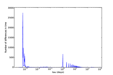
Figure 3: Histogram of the interval between observations for the WFCAMCAL08B data. tau is the interval between any 2 observations regardless of filter and these are binned logarithmically. The peaks at $\sim 10^{-3}$ days are intervals during a $ZYJHK$ sequence and the peaks at $\sim 1$ day and multiples of $1$day are repeat observations on subsequent nights.

On the other hand an analytical expression of FAP for variability indices may depend on the deviation from the mean which will vary according to the survey analysed since it must depend on detector efficiency, number of measurements, magnitude, etc. However, $K_{\rm fi}^{(s)}$ has a weak dependence on the properties of the survey in which Eqn. 15 provides a value above which correlated sources may be distinguished from noise. The only term to be determined is the fractional fluctuation in positive correlated measurements ($f_{\rm fluc}=n_{f}/N_{s}$). From our results, we propose the following empirical equation,

$$f_{\rm fluc}=\frac{n_{f}}{N_{s}}=\alpha-\sqrt{\frac{\beta(\alpha)}{N_{s}}},$$ (16)

i.e. a constant ($\alpha>0$) plus a term related to the number of correlations. The second term in this equation decays quickly to zero as $N_{s}$ increases and it provides a strong cutoff values on data with few epochs. $\beta<\alpha^{2}N_{s}^{Min}$ since the $f_{\rm fluc}$ for $K_{\rm fi}^{(s)}$ must be greater than 0 for any number of correlations. Large values of $\alpha$ give a more complete selection while smaller values result in a more reliable sample. Figure 1 shows the number of sources selected using Eqn. 16 for $s=2$ (black lines) and $s=3$ (grey lines) as a function of $\alpha$ values. Solid lines mark the number of sources of WVSC1 stars, while the dashed lines mark the efficiency of selection (ratio of total number of sources to number of known variables). The total number of sources is normalization by the total number of WVSC1 stars (319) to give an efficiency metric ($E_{tot}$). Table 2 shows the number of total sources selected ($E_{tot}$) and the fraction of WVSC1 stars ($E_{WVSC1}$) for some $\alpha$ values. For instance, to select about $90\%$ of WVSC1 stars we need a sub-sample of $3.77\times 319$ stars using $\alpha=0.30$ for $s=2$. On the other hand to select about $92\%$ of WVSC1 stars we need a sub-sample of $3.71\times 319$ stars using $\alpha=0.48$ for $s=3$.

4.3 $\Delta T$ estimate and correlated observations

The variation of variability indices with $\Delta T$ will depend on many factors such as: the variability period ($P$), the shape of the light curve, the signal-to-noise, and outliers. In order to estimate the influence of $\Delta T$ we simulate a pure sinusoidal variation with a period (P). Next, we compute the $K_{fi}^{(s)}$ indices and see how changing $\Delta T$ as a function of $P$ affects how well we can separate a sinusoidal signal from random noise.

Fig. 2 shows the $K_{\rm fi}^{(s)}$ indices as a function of $\Delta T/P$. $K_{fi}^{(s)}$ decreases quickly to the expected values for random variations when $s=2$, while, when $s=3$, $K_{\rm fi}^{(s)}$ remains higher than the expected noise value for all $\Delta T/P$. This result helps us to understand and use $\Delta\,T$ values. For instance, if $\Delta\,T<0.1P$, we will get large values for $K_{\rm fi}^{s}$, clearly separated from noise and thus detect variability more easily.

Table 2: Efficiency metric for some $\alpha$ values.

s = 2			s = 3
$\alpha$	$E_{WVSC1}$	$E_{tot}$	$\alpha$	$E_{WVSC1}$	$E_{tot}$
0.20	0.57	1.72	0.20	0.31	0.65
0.22	0.66	1.90	0.24	0.41	0.79
0.24	0.72	2.18	0.28	0.50	0.96
0.26	0.78	2.50	0.32	0.64	1.14
0.28	0.84	3.06	0.36	0.71	1.42
0.30	0.90	3.77	0.40	0.80	1.79
0.32	0.93	4.83	0.44	0.88	2.44
0.34	0.95	6.70	0.48	0.92	3.71
0.36	0.99	9.58	0.52	0.95	5.86
0.38	0.99	13.96	0.56	0.98	9.87

$\Delta\,T$ will be determined predominantly by the cadence of the data. For the WFCAMCAL data, a sequence of 3 to 5 filters were observed over a period of $\sim 0.005$ day, and then each pointing reobserved roughly 1 day later, with longer intervals because of weather or seasonal limits on the observations, see Sect 2.1. This is displayed in Fig 3, which shows the histogram of time between subsequent observations. There is a strong peak $\tau\sim 10^{-3}$day which corresponds to a $ZYJHK$ sequence with duration of $\sim 0.005$ day and a second peak at $\sim 1$ day, and a variety of smaller peaks at other durations, often a few days apart (bad weather, non-photometric nights) and a few small ones at long durations of tens or hundreds of days (field not observed because it was too close to the Sun) or on timescales of 0.01 to 0.1 days: days when many calibration fields were taken for test purposes. The best choice of $\Delta T$ should be the minimum duration that encloses the correlated observations, upto the end of the last integration. $\Delta\,T=0.01$day is a sensible choice as it is slightly wider than the typical box size so no observation is missed and allows us to look for variables with $P\geq 0.1$day, although the main sampling peak at $\sim 1$ day may be expected to limit us to $P>0.5$ days from the Nyquist frequency. Since the sampling is not rigidly at 1 day intervals shorter periods are possible. Having correlated sampling at more than 20 times the frequency of the main sampling rate will avoid additional constraints being applied to the period range.

However, if we have equally spaced data, we are severely restricted. If we have $s=2$ correlations and a spacing of $\tau$, then $\Delta\,T\geq 2\tau$ and $P\geq 20\tau$, if $s=2$. Given that at least 2 full periods are required for a confident identification of periodic behaviour, at least 40 observations would be required to constrain a very narrow range of periods. Thus, correlation indices become very inefficient for equally spaced data. Some deep extragalactic surveys have observations designed to maximise depth, so the observations are taken when seeing and sky levels are at the best, so the observation structure can be pseudo-correlated, but not on fixed time scales. In Paper 2 of this series we will discuss indices which work better with uncorrelated observations.

A correlated data set may be expected to have at least half of the $\tau$ values in a peak or small set of peaks (if several filters with slightly different exposure times) at around the correlation frequency and then the main sampling peaks at $\tau_{\rm samp}>20\tau_{\rm cor}$.

When we consider VISTA surveys, e.g. the VVV (Minniti et al., 2010), the data are observed as pawprints, which then get co-added into tiles Cross et al. 2012, so there are always repeat observations on a short time-scale compared to repeat epochs. These observations are also observed almost contemporaneously, with some tiling patterns jumping between different the same jitter on different pawprints before moving onto the next jitter, so the time between pawprints will usually be shorter than the integration time of the pawprint, so these are ideal for correlated indices applied to the pawprints.

Gaia (Bailer-Jones et al., 2013) is another mission where correlated indices will be extremely valuable. The main astrometric instrument observes stars as they transit across 9 strips of detectors with $\tau\sim 5$s. Stars are then reobserved by a second field of view $2$h later or on the next revolution $6$h later or on longer time scales due to the orbit and precession of the spacecraft.

Figure 4: Histograms of the number of correlations $N_{s}$ for $s=2$ and $s=3$ using bins of width 1.

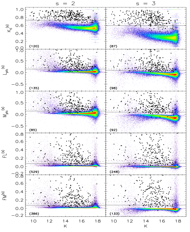
Figure 5: Correlation variability indices versus K magnitude (left diagram) and versus number of correlations (right diagram) in each panel. The maximum number of sources per pixel is displayed in brackets in each panel. The black circles mark the WVSC1 sources and the solid and dashed lines marks the value which encloses $90\%$ and $80\%$ of them.

5 Data analysis

5.1 Broad selection and Bias

From Sects. 4.1, 4.2, and 4.3 we can determine the main constraints on variability analysis. We consider that there is at least one incorrect correlation measurement $n_{f}=1$ in each LC therefore we limit our analyses to sources with more than four correlation measurements, according to Eqn 14. This is the minimum number of correlation measurements adopted in our analysis. Moreover, we adopted $\Delta\,T=0.01$ days, based on the duration of the $ZYJHK$ sequences. By following these constraints, we are considering all LCs that can possibly discriminate a correlated signal from noise with periods of at least greater than $0.1$ days (see Sect. 4.3) We revisited the WFCAMCAL data instead of testing these variability indices using simple sinusoidal light-curves, since this gives a more realistic test with correlated observations, real noise values, and a range of variable types.

Next, we compute the $K_{\rm fi}$, $L_{\rm pfc}$, $M_{\rm pfc}^{(s)}$, $FL^{(s)}$, and $FM^{(s)}$ variability indices using a multi-waveband approach, as discussed in Sect. 3.2 on the data described in Sect. 2.1. Fig. 4 shows the histogram of the number of correlation $N_{s}$ ranging from 1 to 1467 for $s=2$, and from $1$ to $863$ for $s=3$. These numbers are different because the $ZYJHK$ measurements are obtained within a few minutes of each other but not necessarily in all filters. Additionally, the number of correlation measurements decreases quickly for very faint objects around the detection threshold. The total baseline varies from a few months up to three years and the cadence in a single passband can be considered to be quasi-stochastic with rather irregular gaps (see Hodgkin et al., 2009; Cross et al., 2009; Ferreira Lopes et al., 2015, for a better discussion).

5.2 Searching for periodic variations

To search for the best period a Lomb-Scargle periodogram (Lomb, 1976; Scargle, 1982) was computed for each LC. We set the low-frequency limit ($f_{0}$) for each periodogram to be $f_{0}=2/T_{\rm tot}$days^-1, where $T_{\rm tot}$ is the total time spanned by the LC. The high-frequency limit was fixed to $f_{N}=\frac{1}{\Delta\,T}=10$ days^-1, and the periodogram size was scaled to $10^{5}$ elements. Initially, we compute the Lomb-Scargle periodogram independently for each broadband filter ($Y$, $Z$, $J$, $H$, and $K$) as well as for the chromatic light curve (as described in Ferreira Lopes et al. 2015). The use of all broadband filters allows us to find variability periods in the cases where the photometry is high quality in some filters, but not others: e.g. in some filters the object may be saturated (sometimes leading to a non-detection at the correct location), or may be very faint, close to the detection limit or even too faint to be detected.

For each broadband filter as well as for the chromatic light curve we retain the $10$ periods corresponding to the highest peaks. Next these periods were refined following De Medeiros et al. (2013), namely, by maximizing the ratio of the variability amplitudes to the minimum dispersion in the phase diagram given by Dworetsky (1983). Finally, in order to select the very best period, we use the $\chi^{2}$ test, in the same way as described in Ferreira Lopes et al. 2015.

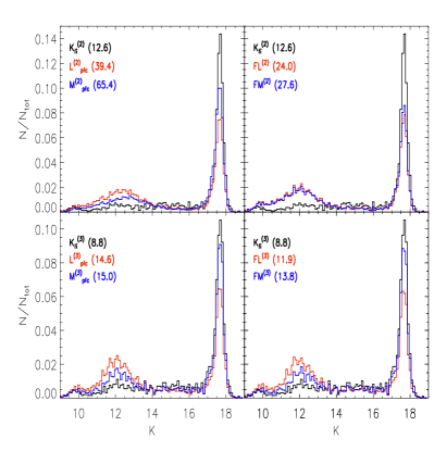
Figure 6: Histograms of the sources selected with a constant cutoff value for $K_{\rm fi}^{(s)}$ (black line), $L^{(s)}_{pfc}$ and $FL^{(s)}$ (red line), and $M^{(s)}_{pfc}$ and $FM^{(s)}$ (blue line) indices normalized for the total number of sources selected in each one of them. $E_{tot}$ values for each index is displayed in parentheses. The upper panel shows the histograms for $s=2$ while the lower panel shows them for $s=3$. The cutoff values were determined considering a value that includes $90\%$ of WVSC1 stars (see Table 3).

6 Results and Discussions

We analyse the efficiency of variability indices for selecting variable stars in the WFCAMCAL database. We evaluate responses of these indices as a function of magnitude and the number of correlations. This study allows us to trace important remarks about the most efficient way to select variable stars. The most efficient index is the one that encloses the majority of the WVSC1 stars with the fewest stars which do not belong to the WVSC1 catalogue and are mostly misclassifications. We compute the variability indices as described in Sect. 3.2. We detail our results in an analysis of correlation variability indices that were computed using a panchromatic approach such as described in Sect. 3.2. Below we present our results using stars from the WVSC1 catalogue as a comparison.

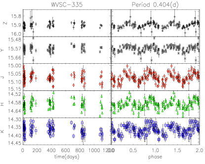
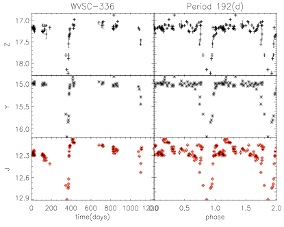
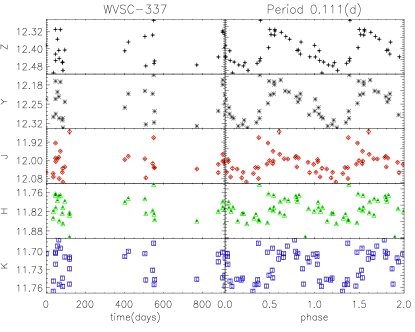
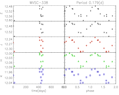
Figure 7: LCs and phase diagrams of C1 catalog. The identifiers and periods are displayed above each panel.

6.1 Efficiency of variability indices

Fig 5 shows the distribution of $K_{\rm fi}$, $L_{\rm pfc}$, $M_{\rm pfc}^{(s)}$, $FL^{(s)}$, and $FM^{(s)}$ variability indices as a function of magnitude and the number of correlations $N_{s}$, for $s=2$ and $s=3$. The solid and dashed lines are set to the values that must be adopted if we want to select $90\%$ and $80\%$ of the final WVSC1 catalogue, respectively. Fig 6 shows the histogram of these indices as a function of magnitude for stars selected using the cutoff value that includes $90\%$ of the WVSC1 catalogue.]

• $K_{\rm fi}^{(s)}$ presents a clear separation of WVSC1 stars from the other stars for $K\leq 17$ mag. The lines that appear for $K\geq 17$ mag are due to the high number of sources with just a few epochs (typically $N_{s}<20$). This index produces discrete values and these are more evident for a small number of epochs. The right panel shows a higher dispersion for low numbers of $N_{s}$ as expected. Statistical fluctuations may provide high contamination in this region despite the number of correlations being above the minimum number that allows us to discriminate them, according to Eqn 14. $K_{fi}^{(3)}$ shows a similar behaviour although it displays a greater separation of WVSC1 stars from the other stars.

• $L_{\rm pfc}^{(s)}$ is equivalent to two previous indices under some constraints: it is equal $J_{\rm WS}$ for $s=2$ and equivalent to $J_{\rm pfc}^{(s)}$ when the correlations are obtained in different filters. $J_{WS}$ has been used in the selection criteria for several surveys (e.g. Christiansen et al., 2008; McCommas et al., 2009; Morales-Calderón et al., 2009; Bhatti et al., 2010; Shappee & Stanek, 2011; Pasternacki et al., 2011).

  $L_{\rm pfc}^{(s)}$ provides a higher selection efficiency than previous indices and it performs combinations among measurements in $\Delta T$ intervals rather than across wavelengths. $L_{\rm pfc}^{(2)}$ indices present a clear separation of WVSC1 stars from other stars. If we assume a constant value of $L_{\rm pfc}^{(s)}$ as a selection criterion we observe that most of the non-variable stars selected are faint stars. The separation between WVSC1 and other stars is clearer for $s=3$ than for $s=2$. Indeed, the number of sources preselected to enclose $90\%$ of WVSC1 stars are about $30\%$ fewer for $s=3$ than $s=2$. Two main features that are expected with increasing $s$ are observed: the increase in the number of stars with negative indices values and a better discrimination between variable and non-variable stars.

• $M_{\rm pfc}^{(s)}$ calculates the median of the correlation values in contrast to the mean encapsulated by $L_{\rm pfc}^{(s)}$. Both mean and median values are used to determine the central or typical value in a statistical distribution. The weight of the outliers is reduced in the median compared to the mean. Outliers in photometric data are commonly associated with variations in brighter stars non-linearity and saturation. On the other hand, the increasing dominance of correlated noise is expected for faint stars as the errors become dominated by the sky noise, rather than photon statistics. Fig. 6 shows a underestimation of $L_{\rm pfc}^{(s)}$) and $M_{\rm pfc}^{(s)}$ indices implying on increase of misclassification. Indeed, the number of stars is higher of $M_{\rm pfc}^{(s)}$ than $L_{\rm pfc}^{(s)}$ for faint stars and against for brighter stars. Fig. 6 shows an increase in the fractions of stars selected at both the bright and faint magnitudes for $L_{\rm pfc}^{(s)}$) and $M_{\rm pfc}^{(s)}$ indices, implying an increase in the misclassification rate. The misclassification rate is higher for faint stars when using $M_{\rm pfc}^{(s)}$ than when using $L_{\rm pfc}^{(s)}$, and vice-versa for bright stars. Therefore stars that match both criteria should have a lower misclassification rate at both the bright and faint ends, so agreement between these indices should be considered as a selection criteria.

  Using larger $s$ values gives less weight to outliers and partially-correlated noise, and this leads to a better estimations of the centre of the distribution for both the mean and median. Therefore, the efficiency of $L_{\rm pfc}^{(s)}$ and $M_{\rm pfc}^{(s)}$ will increase and they tend to have similar $E_{tot}$ values for different indices for higher $s$ especially if sources with small numbers of correlations are removed, as observed in Table 3 for $s=3$ and $N_{s}>20$. Meanwhile, the $K_{\rm fi}^{(s)}$ are the best indices to perform a selection of variable stars, when we only consider higher $s$ values as well as only those sources with $N_{s}>20$ (see Table 3).

• $FL^{(s)}$) and $FM^{(s)}$ provide better efficiency values ($E_{tot}$) among those indices computed from correlation magnitudes (see Table 3). The $F^{(s)}$ factor provides a concentration of non-variables with values around zero as well as a reduction in the spread of bright sources. We observe a reduction of more than $300\%$ on the number of sources pre-selected by $L_{\rm pfc}^{(s)}$ and $M_{\rm pfc}^{(s)}$ indices for $s=2$ and about $20\%$ for $s=3$ (see Fig. 6). The large reduction is not found for $s=3$ because these indices become more accurate with increasing $s$ values and this therefore decreases the weight of $F^{(s)}$. On the other hand, only a slight decrease in $E_{tot}$ was observed when we use as correction factor $K_{\rm WS}/0.789$ (see Table 3). Such factor is used to build the $L_{\rm WS}$ Stetson index (Stetson, 1996) that can be expressed by $L_{\rm WS}\approx L^{(2)}_{\rm pfc}\times K_{\rm WS}/0.789$.

Table 3: Efficiency metric ($E_{tot}$) for variability indices analysed to select $90\%$ and $80\%$ of WVSC1 stars for $N^{(s)}>4$ and $N^{(s)}>20$, respectively.

	$N_{s}>4$		$N_{s}>20$
Index	$E_{tot}(90\%)$	$E_{tot}(80\%)$	$E_{tot}(90\%)$	$E_{tot}(80\%)$
$K_{\rm fi}^{(2)}$	12.6	8.8	4.7	2.9
$K_{\rm fi}^{(3)}$	8.9	5.2	3.0	1.7
$L_{\rm pfc}^{(2)}$	40.1	21.5	27.3	14.7
$L_{\rm pfc}^{(3)}$	14.7	8.8	8.6	5.5
$M_{\rm pfc}^{(2)}$	65.5	29.7	48.4	20.0
$M_{\rm pfc}^{(3)}$	15.0	9.9	7.4	4.9
$FL^{(2)}$	24.0	13.2	14.6	7.9
$FL^{(3)}$	12.0	7.4	6.7	4.4
$FM^{(2)}$	27.6	15.1	16.7	8.9
$FM^{(3)}$	13.8	8.5	6.5	4.0
$L_{\rm WS}$	38.4	20.1	25.6	13.2

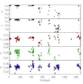
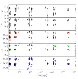
Figure 8: Examples of LCs shown intrumental bias. The identifiers are displayed above each panel.

Summarizing, the correlation variability indices discriminate between uncorrelated and correlated data that is a typical feature of variable stars. We can enclose almost all WVSC1 stars in a sample with fewer than about 1500 sources. These indices still present a low efficiency for discrimination at the faint end or bright end. The root cause in each case may well be different: excess high values for bright sources are due to temporal saturation and few epochs and increases in measurement uncertainties for the faint stars which makes the variability indices more sensitive to statistical fluctuations and systematics.

Figure 6 shows the histograms of sources selected for a constant cutoff value for the higher ranked indices. These indices return most of the WVSC1 stars with fewer non-variable stars (see Table 3). However, these indices have a clear bias on selection from the point of view of magnitude since they are not evenly distributed along all K values. For $s=2$ we observe that $K_{\rm fi}^{(s)}$ (black line) and $FL^{(s)}$ (red line) display a prominent over-selection for faint stars while $FM^{(s)}$ (blue line) is biased for both brighter and faint stars. On the other hand, the three indices have similar bias for $s=3$. Such a result indicates that the efficiency of these indices may be similar for higher $s$ values since the difference in $E_{tot}$ between them is smaller for $s=3$. Indeed, more than $60\%$ of stars with $k>17.5$ have $N_{s}<20$. This low detection efficiency for the instrument in this region gives a maximum magnitude limit where we can sensibly use these indices.

On the other hand, if we use the analytical expression for $f_{\rm fluc,s}$ (see Sect. 4.2) we obtain a higher efficiency. This function allows us to analyse stars with lower $N_{s}$ values (of course, above the minimum number of correlations $N_{s}>4$) with a similar efficiency such as that obtained for $FL^{(s)}$ and $FM^{(s)}$ considering a more strict selection, i.e. $N_{s}>20$. Using $f_{fluc,s}$ we can enclose a greater number of WVSC1 stars with fewer contaminating sources selected (see Table 2). $f_{fluc,s}$ is an empirical relation and it may be adapted according to its purpose.

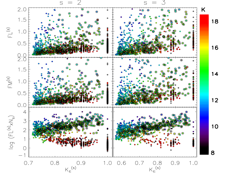
Figure 9: $FL^{(s)}$, $FM^{(s)}$, and logarithmic $FL^{(s)}\times N_{s}$ versus the $K_{\rm fi}^{(s)}$ variability indices for stars selected by $f_{\rm fluc}$ expression using $\alpha=0.30$ for $s=2$ and $\alpha=0.46$ for $s=3$ (see Sect. 6.2) for $s=2$ (left panels) and $s=3$ (right panels). The WVSC1 stars are marked by open black circles and the colours are set by the K magnitude. Objects marked by crosses do not have a K-band magnitude, either being too faint, or saturated. They have measurements in other bands.

6.2 Searching for Variable Stars

We use the $\alpha$ values (see Sect.4.2) in order to select at least $90\%$ of the WVSC1 stars. Therefore, we adopt $\alpha=0.30$ for $s=2$ and $\alpha=0.46$ for $s=3$ which return a combined sample of $1133$ variable stars candidates that were not included in the WVSC1 catalogue. The periods were computed according to Sect. 5.2 and we visually inspected each star. According to our analysis these stars can be divided in to five main groups: (a) variable stars measured in few epochs; (b) variable stars with low signal-to-noise and low confidence periods; (c) variable stars with amplitudes which are near to the noise level; (d) aperiodic variable stars or variables of such long periods that these data were insufficient for deriving them; (e) false variables due to instrumental or reduction problems.

Our procedure has resulted in a catalogue with four new sources (C1). Fig. 7 shows the C1 stars which may be included in abc groups with variability indices’ values near to those expected from noise. Fig. 8 show some instrumental variations that can appear to give false positives for variable stars: false variables due to instrumental saturation (left and middle panels) and for data reduction problems (right panel). The separation between stars of abc and de groups is not possible using only variability indices. Discriminating these sources using statistical analyses will be discussed in a forthcoming paper. Table 4 lists coordinates, periods, mean magnitudes, and the number of epochs in each filter for this sample. WVSC-336 has a period of 192 days but its period may be higher since we don’t observe a complete variability cycle.

6.3 Two-dimensional View of Correlated Data

The $f_{\rm fluc}$ defined for $K_{\rm fi}^{(s)}$ variability indices, using the expression in Eq. 16, presents the best efficiency for selecting WVSC1 stars (see Tables 2 and 3). However it returns a lot of false positives when we have few correlations. The combination of indices based on correlation signals ($K_{\rm fi}^{(s)}$) with those based with correlation values ($FL^{(s)}$ and $FM^{(s)}$) may provide two-dimensional view of correlated data.

Fig. 9 shows the $FL^{(s)}$, $FM^{(s)}$, and logarithmic of $FL^{(s)}\times N_{s}$ as a function of $K_{\rm fi}^{(s)}$ (named KFLs diagram) for $s=2$ (left panels) and $s=3$ (right panels). The KFLs diagrams allow us discriminate two main groups; (G1) faint stars where about $90\%$ have $K_{\rm fi}^{(s)}=1$ due to a small number of correlations; (G2) is composed of stars with $K\leq 16.5$ that includes $91\%$ of WVSC1 stars. These groups display a clear separation if you multiply $FL^{(s)}$ by the number of correlations ($N_{s}$) where $G1$ has $logFL^{(s)}\times N_{(s)}<1.5$ and G2 is delimited by $logFL^{(s)}\times N_{s}>1.5$. However, the last diagram is biased for $N_{s}$ and so comparisons between different sources are difficult to make.

Stars included in G2 with low values of $K_{\rm fi}^{(s)}$ are mainly bright, saturated stars showing a low level of variability and false positive variations due to instrumental bias. The boundary between WVSC1 and other stars is not well defined in this diagram. Nevertheless, the KFLs diagram helps us enclose about $90\%$ of WVSC1 stars with $E_{tot}\sim 2$ in G2.

7 Conclusions

Table 4: Periodic objects in the WFCAM Variable Star Catalog (C1).

ID [WSA]	ID [WVSC]	RA [deg.]	DEC [deg.]	P [d]	$\langle Z\rangle$	$\langle Y\rangle$	$\langle J\rangle$	$\langle H\rangle$	$\langle K\rangle$	$N_{Z}$	$N_{Y}$	$N_{J}$	$N_{H}$	$N_{K}$
858994169008	WVSC-335	+277.0394050	+1.7390500	0.40396	15.903	15.573	15.076	14.593	14.368	80	83	97	94	98
858994205031	WVSC-336	+277.4906120	+1.2348900	192	17.228	15.128	12.294	-9.999	-9.999	68	11	8	0	0
858994439420	WVSC-337	+104.8895590	-4.9367370	0.111042	12.409	12.250	12.017	11.822	11.725	25	21	23	21	32
858994483642	WVSC-338	+129.0526690	-10.2269770	0.178714	12.531	12.490	12.275	12.039	11.984	11	10	11	11	11

From our results we can conclude that: the analysis of databases with fewer than 4 correlated measurements is not possible using $K_{\rm fi}^{(s)}$ and related indices (using factor $F^{(s)}$) when we consider, the case of one wrong value. In these cases we may use $L_{\rm pfc}^{(s)}$ or $M_{\rm pfc}^{(s)}$ indices to discriminate correlated and uncorrelated data. On the other hand, when we have enough correlation measurements, the $K_{\rm fi}^{(s)}$ variability indices provide unique features to do time domain analysis that allows us to define a general way that can be applied to any survey with correlated epochs: it presents a low sensitive to outliers, does not undergo strong variations with magnitude, it has a clear interpretation and a theoretical definition of a value expected for noise, it has a well defined range of values from 0 to 1, and it is not dependent on error bars. Therefore it may be used as a universal method to select correlated variations. Moreover, KFLs diagrams displays two unique variability features related to intensity and number of positive correlated measurements which allow us to improve $E_{tot}$ by at least $40\%$ (see Sect. 6.3).

The $FL^{(s)}$ and $FM^{(s)}$ values in the $KFLs$ diagrams (see Fig. 9) may vary for different surveys. However the $K_{\rm fi}^{(s)}$ is not strongly dependent on instrumental features and its cutoff values can be adopted as universal values as can $f_{\rm fluc,s}$. Its values are related with the discrimination of correlated and uncorrelated data and its response is unbiased with respect to magnitude or observed wavelength. After selecting the variable star candidates using $f_{\rm fluc}$ we may use the $KFLs$ diagrams to improve the selection. Next we can remove G1 stars and use levels of significance of some periodicity methods to discriminate which of these display periodic variations.

This work is the first in a series that make a detailed analysis of all processes of variable photometric data. In this first paper we have investigated which indices give the most efficient selection when we have correlated observations. In the second paper of this series we will consider uncorrelated observations and determine which are the best indices for selecting variable stars. In the coming years we will apply these methods to very large surveys of the Milky Way, e.g. VVV, PanSTARRS, Gaia and in the longer term to LSST to provide fast and reliable classifications of variable stars within the Milky Way, which will improve our understanding of the evolution of different stellar populations and thus the formation of structures within our Galaxy.

8 Acknowledgements

C. E. F. L. acknowledges a post-doctoral fellowship from the CNPq. N. J. G. C. acknowledges support from the UK Science and Technology Facilities Council.

References

- Alard & Lupton (1998) Alard, C. & Lupton, R. H. 1998, ApJ, 503, 325
- Baglin et al. (2007) Baglin, A., Auvergne, M., Barge, P., et al. 2007, in American Institute of Physics Conference Series, Vol. 895, Fifty Years of Romanian Astrophysics, ed. C. Dumitrache, N. A. Popescu, M. D. Suran, & V. Mioc, 201–209
- Bailer-Jones et al. (2013) Bailer-Jones, C. A. L., Andrae, R., Arcay, B., et al. 2013, A&A, 559, A74
- Baluev (2009) Baluev, R. V. 2009, MNRAS, 395, 1541
- Baluev (2013) Baluev, R. V. 2013, MNRAS, 436, 807
- Becker et al. (2004) Becker, A. C., Wittman, D. M., Boeshaar, P. C., et al. 2004, ApJ, 611, 418
- Bhatti et al. (2010) Bhatti, W. A., Richmond, M. W., Ford, H. C., & Petro, L. D. 2010, ApJS, 186, 233
- Blomme et al. (2010) Blomme, J., Debosscher, J., De Ridder, J., et al. 2010, ApJ, 713, L204
- Borucki et al. (2010) Borucki, W. J., Koch, D., Basri, G., et al. 2010, Science, 327, 977
- Christiansen et al. (2008) Christiansen, J. L., Derekas, A., Kiss, L. L., et al. 2008, MNRAS, 385, 1749
- Cincotta et al. (1995) Cincotta, P. M., Mendez, M., & Nunez, J. A. 1995, ApJ, 449, 231
- Clarke (2002) Clarke, D. 2002, A&A, 386, 763
- Corwin et al. (2006) Corwin, T. M., Sumerel, A. N., Pritzl, B. J., et al. 2006, AJ, 132, 1014
- Cross et al. (2009) Cross, N. J. G., Collins, R. S., Hambly, N. C., et al. 2009, MNRAS, 399, 1730
- Cross et al. (2012) Cross, N. J. G., Collins, R. S., Mann, R. G., et al. 2012, A&A, 548, A119
- Damerdji et al. (2007) Damerdji, Y., Klotz, A., & Boër, M. 2007, AJ, 133, 1470
- De Medeiros et al. (2013) De Medeiros, J. R., Ferreira Lopes, C. E., Leão, I. C., et al. 2013, A&A, 555, A63
- Debosscher et al. (2007) Debosscher, J., Sarro, L. M., Aerts, C., et al. 2007, A&A, 475, 1159
- Deeming (1975) Deeming, T. J. 1975, Ap&SS, 36, 137
- Dubath et al. (2012) Dubath, P., Rimoldini, L., Suveges, M., et al. 2012, VizieR Online Data Catalog, 741, 42602
- Dupuy & Hoffman (1985) Dupuy, D. L. & Hoffman, G. A. 1985, International Amateur-Professional Photoelectric Photometry Communications, 20, 1
- Dworetsky (1983) Dworetsky, M. M. 1983, MNRAS, 203, 917
- Eyer (2006) Eyer, L. 2006, in Astronomical Society of the Pacific Conference Series, Vol. 349, Astrophysics of Variable Stars, ed. C. Aerts & C. Sterken, 15