Role of helicity for large- and small-scale turbulent fluctuations

Abstract

Effects of the helicity on the dynamics of turbulent flows are investigated. The aim is to disentangle the role of helicity in fixing the direction, the intensity, and the fluctuations of the energy transfer across the inertial range of scales. We introduce an external parameter $\alpha$ that controls the mismatch between the number of positive and negative helically polarized Fourier modes. We present direct numerical simulations of Navier-Stokes equations from the fully symmetrical case, $\alpha=0$, to the fully asymmetrical case, $\alpha=1$, when only helical modes of one sign survive. We found a singular dependency of the direction of the energy cascade on $\alpha$, measuring a positive forward flux as soon as only a few modes with different helical polarities are present. Small-scale fluctuations are also strongly sensitive to the degree of mode-reduction, leading to a vanishing intermittency already for values of $\alpha\sim 0.1$. If the analysis is restricted to sets of modes with the same helicity sign, intermittency is vanishing for the modes belonging to the minority set, and it is close to that measured on the original Navier-Stokes equations for the other set.

The direction of the energy transfer in a turbulent flow is believed to be determined by the combined effects of all inviscid invariants which depend on the embedding dimensionality and/or on the coupling with external fields, as in conducting or buoyant systems biskamp ; frisch ; lohse_arfm . For fully homogeneous and isotropic turbulence (HIT) in two dimensions, the presence of two positive-definite invariants, energy and enstrophy, leads to a split regime with energy flowing towards large scales (inverse cascade) and enstrophy to small scales (forward cascade) kraichnan_2d ; boff_2d ; tabeling ; 2dreview ; ecke ; prl_massimo . Three-dimensional (3D) Navier-Stokes equations (NSEs) possess two inviscid invariants; energy and helicity, the scalar product of velocity and vorticity moffatt69 ; moffatt92 ; brissaud . Different from the energy, helicity is observed to be preserved by some dissipative events, such as antiparallel vortex reconnection Laing ; Sheeler , and it is not positive definite. As a result, it is not possible to predict the direction of the energy and helicity transfers from fundamental arguments. Numerical simulations, phenomenological arguments, dynamical models, closures, and comparison with the inviscid Gibbs-like equilibrium distribution suggest that both energy and helicity develop a forward cascade in HIT brissaud ; kraichnan ; waleffe ; chen ; chen2 ; ditlevsen ; biferaleh ; EDQNM . On the other hand, it is well known that the external mechanisms such as rotation mininni ; deusebio , confinement celani ; xia , shear dubrulle or coupling with the magnetic field brandenburg might revert the direction of the energy cascade. Strikingly enough, such a reversal of the flux has been predicted and observed also in 3D HIT with explicit breaking of parity invariance, i.e., by restricting the dynamics to a subset of Fourier modes such that the helicity becomes sign definite biferale2012 ; biferale2013 ; herbert , suggesting that inverse energy transfer events are much broader than previously thought and they are potentially present in all flows in nature. Another not understood crucial aspect of fully developed turbulence is intermittency, the tendency of the flow to develop more and more non-Gaussian velocity fluctuation at smaller and smaller scales. It is not known which key degrees of freedom are responsible for such a phenomenon and whether it is crucial to keep all interactions among different scales to preserve it. Consequently, we cannot model it and we cannot predict its degree of universality, i.e., independence of the large-scale configuration. There exist models based on strong mode reduction (shell models biferale_shellmodel ) which preserve many of the intermittent properties of the original Navier-Stokes equations. On the other hand, an increase or decrease of intermittency is observed in numerical simulations of the original 3D equations with a modulation of local or nonlocal Fourier interactions laval . In this Rapid Communication we systematically investigate the effects of helical mode reduction in 3D NSEs. The aim is threefold: We want to explain the role played by helicity in fixing (i) the direction, (ii) the intensity, and (iii) the intermittency of the energy transfer mechanism.

The key tool used is based on a suitable projection of the NSEs allowing one to disentangle, triad by triad, the properties of the energy transfer as a function of the percentage of negative helically polarized modes kept in the simulation. The existence of a control parameter is crucial to address the problem in a quantitative way, tailoring the degrees of freedom retained and removed, without any modeling. We start with the helical decomposition waleffe ; sagaut of the velocity field ${\bm{u}}({\bm{x}})$, expanded in a Fourier series as ${\bm{u}}_{\bm{k}}=u^{+}_{\bm{k}}{\bm{h}}^{+}_{\bm{k}}+u^{-}_{\bm{k}}{\bm{h}}^{-}_{\bm{k}}$, where ${\bm{h}}^{\pm}_{\bm{k}}$ are the eigenvectors of the curl, i.e., $i{{\bm{k}}}\times{\bm{h}}^{\pm}_{\bm{k}}=\pm k{\bm{h}}^{\pm}_{\bm{k}}$. We choose ${\bm{h}}^{\pm}_{\bm{k}}=\hat{\nu}_{\bm{k}}\times\hat{k}\pm i\hat{\nu}_{\bm{k}}$, where $\hat{\nu}_{\bm{k}}$ is a unit vector orthogonal to ${{\bm{k}}}$, satisfying the condition $\hat{\nu}_{\bm{k}}=-\hat{\nu}_{-{\bm{k}}}$, e.g., $\hat{\nu}_{{\bm{k}}}={{\bm{z}}}\times{{\bm{k}}}/||{{\bm{z}}}\times{{\bm{k}}}||$, with any arbitrary vector ${{\bm{z}}}$. In terms of such an exact decomposition of each Fourier mode, the total energy, $E=\int d^{3}x\,|{\bm{u}}({\bm{x}})|^{2}$, and the total helicity, $H=\int d^{3}x\,{\bm{u}}({\bm{x}})\cdot{\bm{\omega}}({\bm{x}})$, are written as

$$E=\sum_{{\bm{k}}}|u^{+}_{\bm{k}}|^{2}+|u^{-}_{\bm{k}}|^{2},\quad H=\sum_{{\bm{k}}}k(|u^{+}_{\bm{k}}|^{2}-|u^{-}_{\bm{k}}|^{2}),$$ (1)

where ${\bm{\omega}}$ is the vorticity (see also Refs. morinishi ; chen for other previous applications of the same decomposition). The nonlinear term of the NSE can be then decomposed in terms of the helical content of the complex amplitudes, $u^{s_{\bm{k}}}_{{\bm{k}}}$ with $s_{\bm{k}}=\pm$ (see Ref. waleffe ). We consider the dynamics of an incompressible flow (${\bm{\nabla}}\cdot{\bf\bm{u}}=0$) determined by the decimated NSE in which a fraction $\alpha$ of the negative helical modes has been switched off footnote . We introduce the projector on positive/negative helical modes as

$${\mathcal{P}}^{\pm}_{{\bm{k}}}\equiv\frac{{\bm{h}}^{\pm}_{\bm{k}}\otimes\overline{{\bm{h}}^{\pm}_{\bm{k}}}}{\overline{{\bm{h}}^{\pm}_{\bm{k}}}\cdot{\bm{h}}^{\pm}_{\bm{k}}},$$ (2)

where $\overline{\bullet}$ denotes the complex conjugate. We define an operator ${D}^{\alpha}$ that projects each wavenumber with a probability $0\leq\alpha\leq 1$,

$${{\bm{u}}}^{\alpha}({\bm{x}})\equiv D^{\alpha}{{\bm{u}}}({\bm{x}})\equiv\sum_{{\bm{k}}}e^{i{\bm{k}}{\bm{x}}}\,{\mathcal{D}}^{\alpha}_{{\bm{k}}}{{\bm{u}}_{\bm{k}}},$$ (3)

where ${\mathcal{D}}^{\alpha}_{{\bm{k}}}\equiv(1-\gamma^{\alpha}_{{\bm{k}}})+\gamma^{\alpha}_{{\bm{k}}}{\mathcal{P}}^{+}_{{\bm{k}}}$ and the random numbers are $\gamma^{\alpha}_{{\bm{k}}}=1$ with probability $\alpha$ or $\gamma^{\alpha}_{{\bm{k}}}=0$ with probability $1-\alpha$. The $\alpha$-decimated Navier-Stokes equations ($\alpha$-NSE) are

$$\partial_{t}{\bm{u}}^{\alpha}=D^{\alpha}[-{\bm{u}}^{\alpha}\cdot{\bm{\nabla}}{\bm{u}}^{\alpha}-{\bm{\nabla}}p^{\alpha}]+\nu\Delta{\bm{u}}^{\alpha},$$ (4)

where $\nu$ is the viscosity and $p$ is the pressure. Notice that the nonlinear terms on the right-hand side of (4) are further projected by ${D}^{\alpha}$ in order to enforce the dynamics on the selected set of modes for all times. Despite the fact that the $\alpha$-NSE break the Lagrangian properties of the nonlinear terms moffatt14 , both energy, $E=\sum_{{\bm{k}}}(|u^{+}_{\bm{k}}|^{2}+(1-\gamma_{{\bm{k}}})|u^{-}_{\bm{k}}|^{2})$, and helicity, $H=\sum_{{\bm{k}}}k(|u^{+}_{\bm{k}}|^{2}-(1-\gamma_{{\bm{k}}})|u^{-}_{\bm{k}}|^{2}),$ are still invariants in the inviscid limit of (4), as in any Galerkin truncation. We can then identify two extreme cases: When $\alpha=0$, we recover the original NSE, and when $\alpha=1$, helicity becomes a coercive quantity with a definite sign. It has been recently shown biferale2012 ; biferale2013 that, in the latter case, the dynamics of (4) develops a double cascade characterized by an inverse energy transfer with a Kolmogorov spectrum $E(k)\sim k^{-5/3}$ for wavenumbers smaller than the forcing scale, $k\ll k_{f}$, and a direct helicity cascade with a $k^{-7/3}$ spectrum for $k\gg k_{f}$. Here we address the questions: Does there exist a critical value $\alpha_{c}$ where the direction of the mean energy transfer suddenly reverses as observed in two-dimensional hydromagnetic systems when changing the forcing mechanisms alexakis , or does the helicity play a singular role? Are a few modes with opposite helical sign enough to transfer energy to small scales ($\alpha_{c}\rightarrow 1$), as suggested in Ref. herbert from considerations based on absolute equilibrium? What happens to small-scale intermittency in the forward cascade regime? Does it depend on the amount of negative/positive helical modes retained? Is the residual small-scale vorticity mainly helical? In order to answer these key questions, we performed a series of numerical simulations at changing $\alpha$ with a fully dealiased, pseudospectral code at resolution up to $1024^{3}$ on a triply periodic cubic domain of size $L=2\pi$. The flow is sustained by a random Gaussian forcing with

$$\langle f_{i}({\bm{k}},t)f_{j}({\bm{q}},t^{\prime})\rangle=F(k)\delta({\bm{k}}-{\bm{q}})\delta(t-t^{\prime})Q_{ij}({\bm{k}}),$$

where $Q_{ij}({\bm{k}})$ is a projector assuring incompressibility and $F(k)=F_{0}k^{-3}$. $F_{0}$ is nonzero only for $|k|\in[k_{\rm min}:k_{\rm max}]$. See Table. 1 for details of the simulations. A different forcing process based on a second-order Ornstein-Uhlenbeck process has also been implemented for some simulations with the same results (not shown). In all cases we have used a fully helical forcing with projection only on ${\bm{h}}^{+}_{\bm{k}}$ in order to ensure a maximal helicity injection rate $h$, independent of the degree of decimation $\alpha$ of the negative helical modes.

RUN	1-8	9-13	14-19	20	21	22
$N$	$256$	$256$	$512$	$512$	$1024$	$1024$
$k_{f}$	$[1,3]$	$[1,3]$	$[1,2]$	$[42,50]$	$[10,12]$	$[1,2]$
$\alpha$	$0-0.999$	$0.1-0.9$	$0-0.9999$	$1.0$	$1.0$	$0$
$F_{0}$	$1.0$	$1.0$	$1.0$	$10.0$	$1.0$	$1.0$

Table 1: $N$: Number of collocation points along each axis. $k_{f}$: forced wavenumbers. $F_{0}$: Forcing amplitude. RUN 1-8: Decimation of only negative helical modes with probability in the range $\alpha\in[0:0.9999]$. RUN 9-13: Same of RUN 1-8 but with either positive or negative helical modes (with $50\%$ probability) removed. RUN 14-19: Similar to RUN 1-8 at higher resolutions. RUN 20-21: Forced at small scales. RUN 22: Same as RUN 1 at higher resolution.

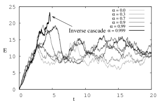
Figure 1: Evolution of energy at varying $\alpha$. All simulations reach a stationary state, except for the case at $\alpha=0.999$, where a constant increase of energy is observed, signaling the existence of a stable inverse energy transfer.

Figure 2: (a) Log-log plot of $E^{+}(k)=\sum_{|{\bm{k}}|=k}|u^{+}_{\bm{k}}|^{2}$ vs $k$ at changing $\alpha$. (b) Log-log plot of $E^{-}(k)=\sum_{|{\bm{k}}|=k}(1-\gamma_{\bm{k}})|u^{-}_{\bm{k}}|^{2}$ vs $k$ at changing $\alpha$. Inset: Rescaled $E^{-}(k)$ with factor $(1-\alpha)$. (c) Semilog plot of flux of energy. Inset: Flux of helicity, at changing $\alpha$.

Energy transfer. We start from the spectral properties of the system following Ref. chen . We define the total spectra restricted to the positive/negative helical modes as $E^{+}(k)=\sum_{|{\bm{k}}|=k}|u^{+}_{\bm{k}}|^{2},E^{-}(k)=\sum_{|{\bm{k}}|=k}(1-\gamma_{\bm{k}})|u^{-}_{\bm{k}}|^{2}$, and the corresponding quantity for the helicity, $H^{\pm}(k)=k\,E^{\pm}(k)$. In the case when both energy and helicity are transferred forward with a rate $\varepsilon$ and $h$, respectively, we expect the usual Kolmogorov 1941 scaling (K41) for both energy and helicity spectra brissaud ; chen ,

$$E(k)\sim C_{E}\varepsilon^{2/3}k^{-5/3},\quad H(k)\sim C_{H}h\varepsilon^{-1/3}k^{-5/3},$$

which reflects in the scaling for each component as

$$E^{\pm}(k)=\varepsilon^{2/3}k^{-5/3}[1\pm Ch(\varepsilon k)^{-1}],$$ (5)

where $C=C_{H}/C_{E}$. In Fig. 1 we show the time evolution of the total energy $E$ starting from a null configuration at $t=0$ when varying the degree of decimation from $\alpha=0$, for the nondecimated NS case, to $\alpha\sim 1$. We notice first that the time needed to develop the initial release of energy becomes longer with increasing $\alpha$, and that the oscillations around the stationary regime are also larger when $\alpha\sim 1$. The most striking phenomenon is that even for a very high decimation of negative helical modes, $\alpha\sim 1$, the system is able to reach a stationary state by transferring energy to the small scales. In other words, it is enough to have very few negative helical modes to develop a stable and stationary positive energy flux. This is quantified in Fig. 2, where we separately plot the spectra for the two helical components for various $\alpha$. The spectrum for the positive helical modes [Fig. 2(a)] is almost unchanged and independent of $\alpha$ with a clearly developed $k^{-5/3}$ slope, whereas the spectrum for the negative helical modes [Fig. 2(b)] tends to react back and become more and more energetic as $\alpha$ increases; this can be explained by looking at the behavior of the energy flux. In Fig. 2(c) we show that the energy flux is constant and independent of $\alpha$ for all $\alpha<1$—it reverts only for $\alpha\sim 1$. The surprising efficiency of the nonlinear transfer suggests that helicity plays a singular role in turbulence: A tiny mixture of positive and negative helical modes axccross all scales is enough to sustain a forward energy. This can be reconducted to the role of the triads with two high-wavenumber modes of opposite helicity waleffe . If this is the case, the most important triads must have one negative and two positive helical modes:

$$S(k|p,q)=\langle({\bm{k}}\cdot u^{-}_{\bm{q}})(u^{+}_{\bm{k}}\cdot u^{+}_{\bm{p}})\rangle+\langle({\bm{k}}\cdot u^{+}_{\bm{p}})(u^{+}_{\bm{k}}\cdot u^{-}_{\bm{q}})\rangle.$$ (6)

They are present with probability $\propto(1-\alpha)$ while triads with two negative helical modes, exist with probability $\propto(1-\alpha)^{2}$. To keep the above triadic correlation constant at decreasing $\alpha$, we must have: $u^{-}_{\bm{k}}\rightarrow u^{-}_{\bm{k}}/(1-\alpha)$ and therefore: $E^{-}(k)=\sum_{|{\bm{k}}|=k}(1-\gamma_{\bm{k}})|u^{-}_{\bm{k}}|^{2}\rightarrow E^{-}(k)/(1-\alpha).$ This prediction is shown to be well realized in the inset of Fig. 2(b), where we show that rescaling $E^{-}(k)$ by a factor $(1-\alpha)$ leads to a good overlap, except for $\alpha\sim 1$, where the fluctuations due to the onset of the inverse energy transfer becomes very large and the above argument possibly breaks down. Thus, negative helical modes act as a bridge for the energy transfer; they receive energy from the large-scale positive modes and release it to the small-scale positive modes; the fewer there are, the more intense their amplitude must be to do it efficiently. When negative helical modes become too rare or absent, i.e., for $\alpha\sim 1$, this bridging is no longer possible and the energy flows upscale biferale2012 . Helicity plays the role of a passive catalyst in the energy transfer. Proving the existence of a unique $\alpha_{c}$ for the inversion of the energy transfer could be extremely hard and it may not be crucial. The observed value is so close to unity that it might also be dependent on the realization of $\gamma_{\bm{k}}$ and/or on the Reynolds numbers. This issue is left for a more detailed analysis in a future work.

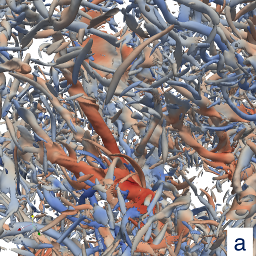
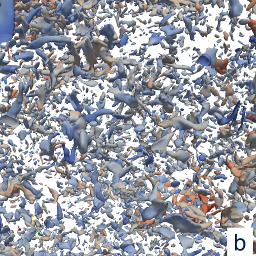
Figure 3: (Color online) Iso-vorticity surfaces for (a) $\alpha=0$, (b) $\alpha=0.5$. The color palette is proportional to the intensity of the helicity, red for high positive values ($\sim 10^{3}$) to blue for high negative values ($\sim-10^{3}$).

Intermittency. The second important problem addressed concerns intermittency, the presence of strong non-Gaussian fluctuations at small scales, usually interpreted as a build up of instabilities in the vortex-stretching mechanisms. Here, we want to understand how intermittency changes under helical mode reduction. A visual inspection of the vorticity field, in Fig. 3, shows a strong depletion of filament-like structures, of the standard 3D NSE [Fig. 3(a)] with decimation of the negative helical modes, shown, e.g., for $\alpha=0.5$ [Fig. 3(b)]. In order to quantitatively assess the degree of intermittency, we focus on the so-called structure functions (SFs), $S^{(p)}(r)={\langle(\delta_{r}u^{\alpha})^{p}\rangle}$, based on the $p$ moments of the transverse velocity increments $\delta_{r}u^{\alpha}=u^{\alpha}_{y}(x+r)-u^{\alpha}_{y}(x)$ as a function of the separation scale (the selection of the $x-y$ components is arbitrary because of isotropy).

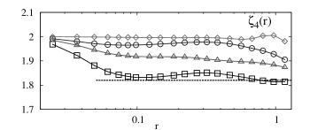
Figure 4: Top panel: Excess kurtosis of transverse SF for $r=\eta$ at changing $\alpha$: ($\square$): decimation of negative helical modes only; ($\bigcirc$): decimation of either positive or negative helical modes with $50\%$ probability; ($\triangle$): a posteriori decimation of negative helical modes from a velocity field of standard nondecimated NSEs. Bottom: Logarithmic local slopes for fourth order moment. $\alpha=0$, i.e., the full NSE ($\square$). $\alpha=0.5$ : The whole field ($\bigcirc$) or its ${\bm{h}}^{+}_{\bm{k}}$ ($\triangle$) and ${\bm{h}}^{-}_{\bm{k}}$ ($\Diamond$) components. The horizontal line represents the standard intermittent correction as predicted from Ref. she .

In Fig. 4 we show (i) the local slopes of the relative scaling of fourth order SF with respect to the second order, $\zeta^{(4)}(r)=d\,log[S^{(4)}(r)]/d\,log[S^{(2)}(r)]$ for the case $\alpha=0.5$, and (ii) the value of the excess kurtosis for $r=\eta$, $K(\eta)=S^{(4)}(\eta)/[S^{(2)}(\eta)]^{2}$, at changing $\alpha$. In the top panel, concerning the kurtosis, we found that intermittency is highly sensitive to $\alpha$ decimation; it is enough to remove a small fraction of negative helical modes from the dynamics to strongly deplete the non-Gaussian character. In the same panel we show also the results of another numerical experiment, where we repeated the measurements in a set of simulations (RUN 9-13) with random decimation; this time either a positive or a negative helical mode is decimated with a probability $\alpha$. The reduction in the intensity of intermittency is comparable with the previous case. To further investigate the role of dynamic helical mode-reduction, we performed a projection aposteriori, applying the operator $D^{\alpha}$ to the velocity field obtained from a fully resolved non-decimated NSE ($\alpha=0$). In this case, intermittency remains almost unchanged, independently of $\alpha$, suggesting that only the dynamical mode reduction is crucial to deplete the vortex-stretching mechanism. In the bottom panel we show the results concerning the local scaling exponent $\zeta^{(4)}(r)$ for $\alpha=0.5$, and we compare it with the original NS case $(\alpha=0)$ and with two other important measurements obtained by taking the velocity configurations dynamically generated with $\alpha=0.5$ and projecting them on their positive or negative helical components, i.e., by applying the projector ${\mathcal{P}}^{+}_{{\bm{k}}}$ or ${\mathcal{P}}^{-}_{{\bm{k}}}$ on all modes. Doing that, we observe intermittency for the projection on the majority component ${\bm{h}}^{+}_{\bm{k}}$ and a vanishingly small correction for the projection on the minority helical component ${\bm{h}}^{-}_{\bm{k}}$. In summary, we can conclude that intermittency as measured from real-space velocity configurations is the results of a highly non-trivial and entangled correlation among a subset of key modes in Fourier space. It is hidden in the correlation among all Fourier modes with given helical components.

Conclusion. We have highlighted and quantified the singular role played by helical Fourier modes in the energy flux reversal, showing that a forward transfer is always preferred as soon as a very small percentage of modes with opposite helicity are present. These findings suggest the possibility to check a posteriori on direct numerical simulations and experiments of strongly rotating flows, of flows under vertical confinement or under strong shear the role played by different helical triadic interactions in driving the energy transfer forward or backward. Intermittency measured on real-space fields is fragile and strongly dependent on the mode-reduction protocol, suggesting that its origins must rely on highly nontrivial correlations among helical and nonhelical fluctuations. In particular, it is apparently key to have all modes with a given helical component. Another key factor might be to keep local or nonlocal interactions in Fourier space, as also suggested by numerical experiments based on a scale-dependent mode-reduction scheme laval .

- (1) D. Biskamp, Magnetohydrodynamic Turbulence (Cambridge University Press, Cambridge, UK, 2003).
- (2) U. Frisch, Turbulence: The Legacy of A.N. Kolmogorov (Cambridge University Press, Cambridge, UK, 1995).
- (3) D. Lohse and K. Q. Xia, Annu. Rev. Fluid Mech. 42, 335 (2010).
- (4) R. H. Kraichnan, Phys. Fluids 10, 1417 (1967).
- (5) G. Boffetta and S. Musacchio, Phys. Rev. E 82, 016307 (2010).
- (6) J. Paret and P. Tabeling, Phys. Fluids 10, 3126 (1998).
- (7) H. J. H. Clercx, and G. J. F. van Heijst, Appl. Mech. Rev. 62, 020802 (2009).
- (8) P. Vorobieff, M. Rivera, and R. E. Ecke, Phys. Fluids 11, 2167 (1999).
- (9) M. Cencini, P. Muratore-Ginanneschi, and A. Vulpiani, Phys. Rev. Lett. 107, 174502 (2011).
- (10) H. K. Moffatt, J. Fluid Mech. 35, 117 (1969).
- (11) H. K. Moffatt and A. Tsinober, Annu. Rev. Fluid Mech. 24, 281 (1992).
- (12) A. Brissaud, U. Frisch, J. Leorat, M. Lesieur, and M. Mazure, Phys. Fluids 16, 1366 (1973).
- (13) C.E. Laing, R. L. Ricca, and D. W. L. Summers, Scientific Reports 5, 9224 (2015).
- (14) M. W. Scheeler, D. Kleckner, D. Proment, G.L. Kindlmann, and W.T.M. Irvine, Proc. Natl. Acad. Sci. 111, 15350 (2014).
- (15) R. H. Kraichnan, J. Fluid Mech. 47, 525 (1971).
- (16) F. Waleffe, Phys Fluids A 4, 350 (1992).
- (17) Q. Chen, S. Chen, and G. L. Eyink, Phys. Fluids 15, 361 (2003);
- (18) Q. Chen, S. Chen, G. L. Eyink, and D. D. Holm, Phys. Rev. Lett. 90, 214503 (2003).
- (19) P. D. Ditlevsen, Phys. Fluids 9, 1482 (1997).
- (20) R. Benzi, L. Biferale, R. M. Kerr, and E. Trovatore, Phys. Rev. E 53, 3541 (1996).
- (21) M. Lesieur and S. Ossia, J. Turbulence 1, 7 (2000).
- (22) P. D. Mininni, A. Alexakis, and A. Pouquet, Phys. Fluids 21, 015108 (2009).
- (23) E. Deusebio and E. Lindborg, J. Fluid Mech. 755, 654 (2014).
- (24) A. Celani, S. Musacchio, and D. Vincenzi, Phys. Rev. Lett. 104, 184506 (2010).
- (25) H. Xia, D. Byrne, G. Falkovich, M. Shats, Nat. Phys. 7, 321 (2011).
- (26) E. Herbert, F. Daviaud, B. Dubrulle, S. Nazarenko, and A. Naso, Europhys. Lett. 100, 44003 (2012).
- (27) A. Brandenburg, Astrophysical J. 550, 824 (2001).
- (28) L. Biferale, S. Musacchio, and F. Toschi, Phys. Rev. Lett. 108, 164501 (2012).
- (29) L. Biferale, S. Musacchio, and F. Toschi, J. Fluid Mech. 730, 309 (2013).
- (30) C. Herbert, Phys. Rev. E 89, 013010 (2014).
- (31) L. Biferale, Annu. Rev. Fluid Mech. 35 441 (2003).
- (32) J. P. Laval, B. Dubrulle and S. Nazarenko, Phys. Fluids 13, 1995 (2001).
- (33) P. Sagaut and C. Cambon, Homogeneous Turbulence Dynamics (Cambridge University Press, Cambridge, UK, 2008)
- (34) Y. Morinishi, K. Nakabayashi, and S. Ren, JSME Int. J. B 44(3), 410 (2001).
- (35) The choice of decimating negative mode is purely arbitrary nothing would change by decimating positive modes.
- (36) H. K. Moffatt, J. Fluid Mech. 741, R3 (2014).
- (37) K Seshasayanan, S. J. Benavides, and A. Alexakis, Phys. Rev. E 90, 051003 (2014).
- (38) Z.-S. She and E. Leveque Phys. Rev. Lett. 72, 336 (1994).