Bose-Einstein condensation and critical behavior of two-component bosonic gases

Abstract

We study Bose-Einstein condensation (BEC) in three-dimensional two-component bosonic gases, characterizing the universal behaviors of the critical modes arising at the BEC transitions. For this purpose, we use field-theoretical (FT) renormalization-group (RG) methods and perform mean-field and numerical calculations. The FT RG analysis is based on the Landau-Ginzburg-Wilson $\Phi^{4}$ theory with two complex scalar fields which has the same symmetry as the bosonic system. In particular, for identical bosons with exchange $\mathbb{Z}_{2}$ symmetry, coupled by effective density-density interactions, the global symmetry is ${\mathbb{Z}}_{2,e}\otimes{\rm U}(1)\otimes{\rm U}(1)$. At the BEC transition it may break into ${\mathbb{Z}}_{2,e}\otimes{\mathbb{Z}}_{2}\otimes{\mathbb{Z}}_{2}$ when both components condense simultaneously, or to ${\rm U}(1)\otimes{\mathbb{Z}}_{2}$ when only one component condenses. This implies different universality classes for the corresponding critical behaviors. Numerical simulations of the two-component Bose-Hubbard model in the hard-core limit support the RG prediction: when both components condense simultaneously, the critical behavior is controlled by a decoupled XY fixed point, with unusual slowly-decaying scaling corrections arising from the on-site inter-species interaction.

I Introduction

Experiments with cold atomsCW-02 ; Ketterle-02 ; BDZ-08 have provided the opportunity to investigate Bose-Einstein condensation (BEC) in dilute interacting atomic gases. In the BEC a macroscopic number of bosonic atoms, the so-called condensate, occupy the lowest-energy quantum state at a finite temperature. The phase of the condensate wave function provides the order parameter at the transition. BEC transitions are generically expected to belong to the three-dimensional (3D) XY universality class, which is characterized by the spontaneous breaking of an Abelian U(1) symmetry. The same universal critical behavior is observed in the superfluid transition in ⁴He, Lipa-etal-96 ; CHPV-06 in transitions characterized by density or spin waves (as it occurs in some liquid crystals), in magnetic systems with easy-plane anisotropy, etc. PV-02 The XY behavior at the 3D BEC transition has been supported by experimental measurements of the diverging correlation length in a cold-atom bosonic gas. DRBOKS-07 Cold-atom experiments have been extended to mixtures of homonuclear and heteronuclear bosonic gases,PhysRevLett.78.586 ; PhysRevLett.81.1539 ; PhysRevLett.82.2228 ; PhysRevA.63.051602 ; PhysRevLett.99.190402 ; PhysRevLett.103.245301 ; PhysRevLett.105.045303 ; PhysRevA.80.023603 ; PhysRevA.82.033609 ; Nature.396.345 ; PhysRevLett.85.2413 ; PhysRevLett.89.053202 ; PhysRevLett.89.190404 ; PhysRevLett.99.010403 ; PhysRevA.77.011603 ; PhysRevLett.100.210402 ; PhysRevLett.101.040402 ; PhysRevA.79.021601 ; PhysRevA.84.011610 which also show BEC phenomena. Several theoretical studies have discussed various aspects of the behavior of mixtures of bosonics gases, see, e.g., Refs. HS-96, ; Boninsegni-01, ; AHDL-03, ; DDL-03, ; KS-03, ; PC-03, ; KG-04, ; KPS-04, ; ICSG-05, ; PSP-08, ; SCPS-09, ; HSH-09, ; CSPS-10, ; FHRSB-11, ; Pollet-12, ; ACV-14, ; LCD-14, ; GBS-15, , such as low-dimensional behaviors, magnetic-like behaviors at the $n=1$ Mott phases, etc. However, some issues call for further investigations, such as the critical behaviors at the finite-temperature normal-to-superfluid transitions which arise from different BEC patterns.

In this paper we study BEC in mixture of 3D bosonic gases, focussing on the critical behaviors at the finite-temperature transitions arising from BEC. In particular, we consider a system of two identical boson gases with density-density interactions. Equivalently, we may interpret this system as made up by a single two-component boson gas. An example is provided by the lattice two-component Bose-Hubbard (2BH) model

$$H = -t\sum_{s}\sum_{\langle{\bm{x}\bm{y}}\rangle}(b_{s\bm{x}}^{\dagger}b_{s\bm{y}}+{\rm h.c})-\mu\sum_{s\bm{x}}n_{s\bm{x}}$$

$$+ \frac{1}{2}V\sum_{s\bm{x}}n_{s\bm{x}}(n_{s\bm{x}}-1)+U\sum_{\bm{x}}n_{1\bm{x}}n_{2\bm{x}},$$

where $\langle{\bm{x}\bm{y}}\rangle$ indicates the nearest-neighbor sites of a cubic lattice, the subscript $s$ labels the two species, and $n_{s\bm{x}}\equiv b_{s\bm{x}}^{\dagger}b_{s\bm{x}}$ is the density operator. The Hamiltonian is symmetric under U(1) transformations acting independently on the two species and under the ${\mathbb{Z}}_{2}$ transformation exchanging the two bosons. The two-component boson gas shows a quite complex phase diagram in the space of the model parameters, i.e., the temperature $T$, the chemical potential $\mu$, and the on-site couplings $U$ and $V$. In the following we set $t=1$ for the hopping parameter without loss of generality.

We investigate the critical behavior of systems like the 2BH model by field-theoretical (FT) renormalization-group (RG) methods, mean-field and numerical approaches. We show that transitions in these two-component systems may be associated with different spontaneous breakings of the global symmetry

$${\mathbb{Z}}_{2,e}\otimes{\rm U}(1)\otimes{\rm U}(1).$$ (2)

This symmetry may break to ${\mathbb{Z}}_{2,e}\otimes{\mathbb{Z}}_{2}\otimes{\mathbb{Z}}_{2}$ when both components condense simultaneously, or to ${\rm U}(1)\otimes{\mathbb{Z}}_{2}$ when only one component condenses, with two different universality classes for the corresponding critical behaviors.

When both components condense simultaneously, the RG analysis shows that the critical behavior is controlled by a decoupled 3D XY fixed point (FP). Thus, the transition belongs to the 3D XY universality class associated with the symmetry breaking U(1)$\to$${\mathbb{Z}}_{2}$. However, the irrelevant density-density interaction between the two components gives rise to scaling corrections that decay very slowly, as $\xi^{\,-0.022}$, where $\xi$ is the diverging length scale at the transition. Such scaling corrections are not present in standard transitions belonging to the XY universality class, such as at the BEC transition of a single bosonic species.CN-14 ; CTV-13 ; CR-12 ; CPS-07 In that case, scaling corrections decrease significantly faster, as $\xi^{\,-0.78}$. If, instead, only one component condenses, the RG analysis predicts a different critical behavior, which belongs to the same universality class as that of the continuous transitions in chiral models with O$(2)\otimes$O$(2)$ symmetry.Kawamura-88 We also present a RG analysis of the behavior of mixtures of nonidentical bosons with density-density interactions. In this case the phase diagram is characterized by the presence of bicritical or tetracritical points where various transition lines meet.

The paper is organized as follows. In Sec. II we present the RG analysis of the Landau-Ginzburg-Wilson (LGW) theory, which is expected to describe the critical transitions in two-component bosonic systems with density-density interactions. In Sec. III we discuss the phase diagram of the 2BH model (I) in the mean-field approximation. Sec. IV is devoted to a numerical study of the 2BH model in the hard-core, $V\to\infty$, limit. At the transition both components condense. We show that the results can be explained by a 3D XY critical behavior with slowly-decaying scaling corrections, as predicted by the RG analysis. Finally, in Sec. V we draw our conclusions.

II Field-theoretical renormalization-group analysis

We wish now to classify the finite-temperature transitions in the phase diagram of systems consisting of two identical boson species with density-density interactions. For this purpose, we study the RG flow of the effective LGW $\Phi^{4}$ theory associated with the critical modes.Aharony-76 ; ZJ-book ; PV-02 ; v-07 Within the FT RG approach, one first identifies the order parameter. Then, one considers the $\Phi^{4}$ Hamiltonian with the most general fourth-order potential in the order parameter that has the same symmetry properties as the original system. The possible critical behaviors are determined by the stable FPs of the RG flow. Each of them corresponds to a different universality class, associated with the symmetry breaking that occurs in the parameter region in which the FP is located. The stable FPs determine the universal scaling properties, such as the critical exponents, the scaling functions, etc. Note that only systems which are in the attraction domain of the stable FPs undergo continuous transitions. Systems corresponding to LGW theories with parameters that are outside the FP attraction domains, or that belong to the instability region, are predicted to undergo first-order transitions.

At a BEC transition, the condensate behaves like the magnetization in magnetic systems, i.e., $\langle b_{s{\bm{x}}}\rangle\sim(T_{c}-T)^{\beta}$ as $T_{c}$ is approached from below. Critical modes develop a diverging length scale $\xi\sim|T-T_{c}|^{-\nu}$, while the two-point function at the critical point decays algebraically asZJ-book ; PV-02 $G({\bm{x}})\sim|{\bm{x}}|^{-1-\eta}$. The exponents $\beta$, $\nu$, and $\eta$ are universal—they only depend on the universality class—and are related by the scaling relation $\beta=\nu(1+\eta)/2$.

II.1 LGW theory for two-component boson gases

In the case of a mixture of bosonic gases, we associate a complex field $\varphi_{s}({\bm{x}})$, $s=1,2$, with each bosonic species. Since we consider finite-temperature transitions of 3D quantum systems, we must consider a three-dimensional LGW model. As mentioned in the introduction, the relevant symmetry of the systems we consider, such as the 2BH model (I), is ${\mathbb{Z}}_{2,e}\otimes{\rm U}(1)\otimes{\rm U}(1)$. The Hamiltonian is therefore

$${\cal H}_{\rm LGW} = \int d^{3}x\,\Bigl{[}\sum_{s,\mu}|\partial_{\mu}\varphi_{s}({\bm{x}})|^{2}+r\sum_{s}|\varphi_{s}({\bm{x}})|^{2}$$

$$+ g\sum_{s}|\varphi_{s}({\bm{x}})|^{4}+2u\,|\varphi_{1}({\bm{x}})|^{2}|\varphi_{2}({\bm{x}})|^{2}\Bigr{]},$$

where the potential is the most general one under symmetry (2). The Hamiltonian is bounded from below for $g>0$ and $g+u>0$. The quartic couplings $g$ and $u$ are related to the intra-species $V$ and inter-species $U$ on-site couplings of the 2BH model (I). In particular, $u$ must vanish when $U$ vanishes, leaving two decoupled LGW theories, one for each bosonic gas.

General information on the phase diagram of model (II.1) can be inferred by a straightforward mean-field analysis, e.g., by determining the minima of the potential

$$V(\varphi) = r\sum_{s}|\varphi_{s}|^{2}+g\sum_{s}|\varphi_{s}|^{4}+2u|\varphi_{1}|^{2}|\varphi_{2}|^{2}.$$ (4)

For $r>0$ the potential is minimized by $\varphi_{s}=0$, while for $r<0$ the minimum depends on the sign of $w\equiv g-u$. If $w>0$, the minimum occurs when both field components condense, i.e., for $\langle\varphi_{1}\rangle=\langle\varphi_{2}\rangle\neq 0$. This implies the symmetry-breaking pattern

$${\mathbb{Z}}_{2,e}\otimes{\rm U}(1)\otimes{\rm U}(1)\to{\mathbb{Z}}_{2,e}\otimes{\mathbb{Z}}_{2}\otimes{\mathbb{Z}}_{2},$$ (5)

i.e., each U(1) group breaks into ${\mathbb{Z}}_{2}$. Instead for $w<0$, we have $\langle\varphi_{1}\rangle\neq 0$ and $\langle\varphi_{2}\rangle=0$, or viceversa. Thus, the exchange symmetry and only one of the two U(1) groups are broken, so that

$${\mathbb{Z}}_{2,e}\otimes{\rm U}(1)\otimes{\rm U}(1)\to{\rm U}(1)\otimes{\mathbb{Z}}_{2}.$$ (6)

On the boundary line $w=0$, the LGW theory (II.1) is equivalent to the O(4) vector model.

II.2 RG flow and critical behaviors

The LGW theory (II.1) is a particular case of the so-called $MN$ model Aharony-76 ; PV-02

$$\int d^{3}x\Bigl{[}\sum_{ai}(\partial_{\mu}\phi_{ai})^{2}+r\phi_{ai}^{2}+\sum_{ijab}(v_{1}+v_{2}\delta_{ij})\phi_{ai}^{2}\phi^{2}_{bj}\Bigr{]},$$ (7)

where $\phi_{ai}$ is an $M\times N$ matrix, i.e., $a=1,\ldots,N$ and $i=1,\ldots,M$. Indeed, Hamiltonian (II.1) reduces to (7) for $M=N=2$, if we set $\phi_{1i}={\rm Re}\,\varphi_{i}$, $\phi_{2i}={\rm Im}\,\varphi_{i}$, and

$$g=v_{1}+v_{2},\qquad u=v_{1},\qquad w\equiv g-u=v_{2}.$$ (8)

The RG flow of the $MN$ models has been studied by various FT methods.Aharony-76 ; PV-02 ; PV-05 A sketch of the RG flow in the case $M=N=2$ is shown Fig. 1. There are several FPs in the plane of the renormalized quartic couplings $v_{1}$ and $v_{2}$: PV-05 (i) the trivial Gaussian FP for $v_{1}=v_{2}=0$ which is unstable against both quartic perturbations present in Hamiltonian (7); (ii) the O(4)-symmetric FP for $v_{2}=0$ and $v_{1}>0$ which is unstable with respect to the quartic term proportional to $v_{2}$ in Eq. (7); (iii) a stable decoupled XY FP with $v_{1}=0$ and $v_{2}>0$, with attraction domain in the region $v_{2}>0$; (iv) a stable FP for $v_{2}<0$ with attraction domain in the region $v_{2}<0$.

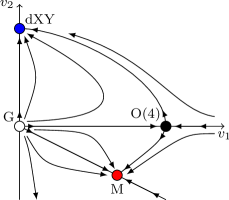
Figure 1: Sketch of the RG flow of the $MN$ model (7) for $M=N=2$. The relevant stable FPs are the decoupled XY FP (dXY), corresponding to FP (iii) in the list reported in the text, and FP $M$, corresponding to FP (iv).

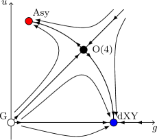
Figure 2: Sketch of the RG flow of the LGW theory for a mixture of two identical bosonic gases. The relevant stable FPs are the decoupled XY FP (dXY), which controls the RG flux for $g-u>0$ (in this case the exchange symmetry is conserved), and a second FP (Asy), relevant for $g-u<0$ (the exchange symmetry is broken).

It is also possible to map the LGW theory (II.1) onto the chiral LGW theory with O($N)\otimes$O($M$) symmetry defined by Kawamura-88 ; CPPV-04 ; PRV-01

$$\int d^{3}x \Bigl{\{}\sum_{ai}[(\partial_{\mu}\phi_{ai})^{2}+r\phi_{ai}^{2}]+{(u_{0}-v_{0})}\sum_{aij}\phi^{2}_{ai}\phi^{2}_{aj}+$$ (9)

$${v_{0}}\sum_{abij}\phi_{ai}\phi_{bi}\phi_{aj}\phi_{bj}\Bigr{\}},$$

where $\phi_{ai}$ is an $M\times N$ matrix. The two models are equivalent for $M=N=2$, if we identify fields and couplings as follows:

$$\phi_{11} = {1\over\sqrt{2}}({\rm Re}\,\varphi_{1}-{\rm Im}\,\varphi_{2}),$$

$$\phi_{12} = {1\over\sqrt{2}}({\rm Im}\,\varphi_{1}-{\rm Re}\,\varphi_{2}),$$

$$\phi_{21} = {1\over\sqrt{2}}({\rm Im}\,\varphi_{1}+{\rm Re}\,\varphi_{2}),$$

$$\phi_{22} = {1\over\sqrt{2}}({\rm Re}\,\varphi_{1}+{\rm Im}\,\varphi_{2}),$$ (10)

and $g=u_{0}-v_{0}/2$, $u=u_{0}+v_{0}/2$. Note that the couplings of the chiral and of the $MN$ model are related by $v_{0}=-v_{2}$ and $u_{0}=v_{1}+v_{2}/2$, so that the FP (iv) mentioned above corresponds to the chiral FP that has been extensively discussed in Refs. Kawamura-88, ; PRV-01, ; CPPV-04, ; foot-controversy, .

According to the correspondence (8), the equivalent model (II.1) presents two stable FPs with attraction domains separated by the line $w=g-u=0$, along which the unstable O(4)-symmetric FP is located. The corresponding RG flows are sketched in Fig. 2.

If $w>0$ the finite-temperature transition is characterized by the simultaneous condensation of both species. The stable FP which determines the critical behavior is located along the line $u=0$, thus representing two decoupled U(1)-symmetric models. This implies that it belongs to the 3D XY universality class, whose critical exponents are CHPV-06 ${\nu_{\textsc{xy}}}=0.6717(1)$ and ${\eta_{\textsc{xy}}}=0.0381(2)$. However, scaling corrections decay much slower than in the U(1)-symmetric theory with a single complex field, where the leading irrelevant perturbation has RG dimension $y_{g}\equiv-{\omega_{\textsc{xy}}}=-0.785(20)$.CHPV-06 ; PV-02 This is related to the RG dimension at the decoupled XY FP of the interaction operator between the two complex order parameters. Since the RG dimension of the energy operator $\int d^{3}x\,\phi^{2}$ is $1/{\nu_{\textsc{xy}}}$, the RG dimension of the interspecies interaction operator $\int d^{3}x\,|\varphi_{1}|^{2}|\varphi_{2}|^{2}$ is

$$y_{u}=2/{\nu_{\textsc{xy}}}-3=-0.0225(4).$$ (11)

Since $y_{u}<0$, this result implies that the perturbation is irrelevant at the decoupled XY FP. However, since $\omega_{u}\equiv-y_{u}$ is very small, the scaling corrections, that behave as $\xi^{-\omega_{u}}=\xi^{-0.0225}$, decay very slowly.

If the coupling $w$ is negative, only one bosonic component is expected to condense. In this case the transition is characterized by the symmetry breaking (6). Therefore, if the BEC transition is continuous, the critical behavior must belong to another universality class, different from the XY one. The corresponding FP has been extensively studied within the equivalent O(2)$\otimes$O(2) LGW theory.Kawamura-88 ; PRV-01 ; CPPV-04 Estimates of the corresponding critical exponents are: (i) $\nu=0.57(3)$ and $\eta=0.09(1)$ from the resummation of the six-loop expansion within the massive zero-momentum scheme;PRV-01 (ii) $\nu=0.65(6)$ and $\eta=0.09(4)$ from five-loop calculations within the minimal subtraction renormalization scheme.CPPV-04 These theoretical results are also supported by experiments, see e.g., Ref. PV-02, and references therein.foot-controversy Therefore, the stable FP of the LGW theory (II.1) with attraction domain in the region $w<0$ is characterized by the critical exponents $\nu\approx 0.6$ and $\eta\approx 0.1$. Of course, models which are outside the attraction domain of the FP are expected to undergo a first-order phase transition.

We finally mention that the critical exponents of the unstable O(4)-symmetric FP along the separatrix $w=0$ are HV-11 ; Hasenbusch-01 $\nu=0.750(2)$ and $\eta=0.0360(3)$. This FP is unstable because the spin-4 perturbation present when $w\not=0$ has positive RG dimension $y_{w}=0.125(5)$ at the O(4) FP. HV-11 ; CPV-03 Thus, an O(4) critical behavior can only be observed by performing a proper tuning of the parameters of the model.

In the following sections we study model (I) in the hard-core $V\to+\infty$ limit. Since the intra-species $V$ is naively related to the quartic coupling $g$, we expect $g$ to be large in this limit, so that $w\equiv g-u>0$. Therefore, the BEC transition should be characterized by the simultaneous condensation of both components, and controlled by the decoupled FP, with a low-temperature phase in which both components condense. Scaling corrections, due to the on-site density-density interaction between the two components, decay very slowly. We also expect such corrections to be larger when the inter-species on-site interaction is attractive, i.e., for $U<0$, while they should be small in the opposite case $U>0$. This is also suggested by the fact that the hard-core 2BH model becomes equivalent to the one-component model in the limit $U\to+\infty$. Therefore, for $U\to+\infty$ we expect a standard XY transition without slowly-decaying $O(\xi^{-{\omega_{u}}})$ scaling corrections.

II.3 Multicritical behavior for two unequal bosonic gases

Figure 3: Different phase diagrams for two interacting bosonic gases. Thin lines indicate continuous transitions, while the thick line represents first-order transitions. RG analyses predict that only in the tetracritical case (left panel) may one have a continuous multicritical behavior at the intersection of the transition lines.

We now discuss a system of two unequal bosonic species, such as that described by the more general BH model

$$H = -\sum_{s}t_{s}\sum_{\langle{\bm{x}y}\rangle}(b_{s\bm{x}}^{\dagger}b_{s\bm{y}}+{\rm h.c})-\sum_{s}\mu_{s}\sum_{\bm{x}}n_{s\bm{x}}\quad$$

$$+ \sum_{s}\frac{1}{2}V_{s}\sum_{\bm{x}}n_{s\bm{x}}(n_{s\bm{x}}-1)+U\sum_{\bm{x}}n_{1\bm{x}}n_{2\bm{x}}.$$

In this case we expect a more complex phase diagram, showing various phases with transition lines along which only one bosonic component condenses, and multicritical points (MCPs), where the critical behavior arises from the competition of the two distinct U(1) orderings. More specifically, a MCP should be observed at the intersection of the normal-to-superfluid transition lines where one of the components condenses.

The LGW theory describing the competition of the two different U(1) orderings of the model (II.3) is obtained by constructing the most general $\Phi^{4}$ theory of two complex fields $\varphi_{s}({\bm{x}})$, with an independent U(1) symmetry for each component, without exchange symmetry. It reads

$${\cal H}_{\rm LGW} = \int d^{3}x\,\Bigl{[}\sum_{s,\mu}|\partial_{\mu}\varphi_{s}|^{2}+\sum_{s}r_{s}|\varphi_{s}|^{2}$$

$$+ \sum_{s}g_{s}|\varphi_{s}|^{4}+2u\,|\varphi_{1}|^{2}|\varphi_{2}|^{2}\Bigr{]},$$

where now we have two quadratic parameters $r_{1}$ and $r_{2}$ and three quartic parameters $g_{1}$, $g_{2}$, and $u$. The multicritical behavior arising from the competition of the two distinct U(1) orderings is determined by the RG flow when both quadratic parameters $r_{1}$ and $r_{2}$ are simultaneously tuned to their critical values, keeping the quartic parameters $g_{1}$, $g_{2}$ and $u$ fixed.

The phase diagram of the most general theory, in which the associated symmetries are O($n_{1}$) and O($n_{2}$), has already been investigated within the mean-field approximation.NKF-74 ; KNF-76 ; CPV-03 Several different phase diagrams have been identified, characterized by three or four transition lines meeting at a MCP, characterized by the presence or the absence of a mixed phase, in which both fields condense. In Fig. 3 we show the phase diagrams corresponding to the case of two coupled U(1)-symmetric theories, in the $T$-$S$ plane where $S$ represents a second relevant parameter (for instance, the difference of the chemical potentials of the two species) that must be tuned to obtain the multicritical behavior. In the LGW theory the two behaviors are determined by the sign of $\Delta\equiv g_{1}g_{2}-u^{2}$. If $\Delta>0$, four critical lines meet at the MCP (tetracritical behavior), as in the left panel of Fig. 3, while, if $\Delta<0$, two critical lines and one first-order line (bicritical behavior) are present, see the right panel of Fig. 3.

The sign of $\Delta$ also controls the nature of the behavior at the MCP. The FT analysis Aharony-02 ; CPV-03 of the LGW theory (II.3) shows that the system undergoes a first-order transition at the MCP for $\Delta<0$, i.e., in the bicritical case, as no stable FP is found in this parameter region. In the opposite case (tetracritical phase diagram) a continuous transition is possible at the MCP, controlled by the decoupled XY FP.

III Mean-field phase diagram of the 2BH model

The phase diagram of the 2BH model (I) can be studied in the mean-field approximation, using

$$b^{\dagger}_{s\bm{x}}b_{s\bm{y}} =\left[(b^{\dagger}_{s\bm{x}}-\phi_{s}^{*})+\phi_{s}^{*}\right]\left[(b_{s\bm{y}}-\phi_{s})+\phi_{s}\right]$$ (14)

$$\approx\phi_{s}b^{\dagger}_{s\bm{x}}+\phi_{s}^{*}b_{s{\bm{y}}}-|\phi_{s}|^{2},$$

where $\phi_{s}=\langle b_{s\bm{x}}\rangle$ are two complex space-independent variables, that play the role of order parameters at the BEC transitions. Approximation (14) allows us to rewrite Hamiltonian (I) as a sum of decoupled one-site Hamiltonians

$$H[\phi_{s}]=-2DJ\sum_{s}\left(\phi_{s}b^{\dagger}_{s}+\phi_{s}^{*}b_{s}-|\phi_{s}|^{2}\right)$$ (15)

$$-\mu\sum_{s}n_{s}+\frac{V}{2}\sum_{s}n_{s}(n_{s}-1)+Un_{1}n_{2}.$$

The spectrum of the theory is invariant under the redefinition $b_{s}\to U_{s}b_{s}$, where $U_{s}$ are two arbitrary phases. Therefore, there is no loss of generality if the two parameters $\phi_{s}$ are assumed to be real. They are determined by minimizing the single-site free energy with respect to $\phi_{s}$.

In the hard-core limit, since $n_{s}=0,\,1$, the mean-field Hamiltonian (15) is defined on a Hilbert space of dimension 4. In the soft-core case, we may have any occupation number, so that the Hilbert space has infinite dimension. In practice, we only consider states such that $n_{s}\leq n_{\rm max}$, checking that typical occupation numbers are significanly lower than $n_{\rm max}$ and verifying that the results are stable with respect to changes of the cut-off $n_{\rm max}$.

Figure 4: Zero-temperature $U$-$\mu$ phase diagram of the 2BH model in the hard-core $V\to\infty$ limit.

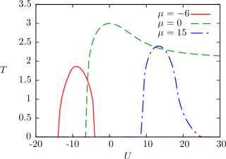
Figure 5: Phase diagram of the hard-core 2BH model for $\mu=-6,\,0,\,15$ in the $U$-$T$ plane. In particular, we show the normal-to-superfluid transition lines.

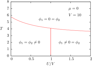
Figure 6: Phase diagram of the 2BH model for $V=10$ and $\mu=0$ in the $U$-$T$ plane. The transitions along the line $U/V=1$ separating the two low-temperature phases are of first order.

In Fig. 4 we report $|\phi_{1}|^{2}=|\phi_{2}|^{2}$ for the hard-core model at $T=0$ as a function of $U$ and $\mu$. The parameter space is divided into four regions: a central one (superfluid domain) in which $|\phi|^{2}\not=0$, and three regions in which $|\phi|^{2}=0$ that differ by the value of the total occupation number $n=n_{1}+n_{2}$. There is a vacuum region in which $n=0$ and two Mott incompressible phases with $n=1$ and $n=2$. The $n=1$ Mott phase presents several interesting features related to the isospin degrees of freedom per site, which may be described by effective low-energy spin Hamiltonians.KS-03 ; DDL-03 ; AHDL-03 ; ICSG-05 The superfluid domain for $\mu<0$, separating the $n=0$ and $n=2$ Mott phases, extends in a strip around the line $U=2\mu$ that gets narrower as $\mu$ decreases (the $n=2$ Mott phase cannot include the line $U=2\mu$ where the on-site interactions would cancel for $n_{1}=n_{2}=1$). This mean-field phase diagram appears quite similar to that of the 1D Hubbard model which can be exactly solved, see, e.g., Refs. 1DHM, ; ACV-14, (we recall that the 1D hard-core 2BH model can be exactly mapped onto the 1D fermion Hubbard model).

The mean-field calculations can be extended to finite temperatures by minimizing the free-energy density

$$f(\phi,\beta)=-\frac{1}{\beta}\ln\mathcal{Z}(\phi,\beta),\quad\mathcal{Z}(\phi,\beta)=\sum_{i}e^{-\beta E_{i}},$$ (16)

with respect to the variational parameters $\phi_{s}$. $E_{i}$ are the energy levels of the single-site Hamiltonian. The finite-temperature phase boundaries are obtained by looking for the smallest value of $\beta\equiv 1/T$ for which, at any given $U$ and $\mu$, $\phi_{s}$ assume non-zero values.

The phase diagrams in the hard-core limit are shown in Fig. 5 for some values of the chemical potential $\mu$. In all cases the low-temperature superfluid phases are characterized by the simultaneous condensation of both components. In particular, for $\mu=0$, the case we will investigate numerically, there is a low-temperature superfluid phase for $U>-6$, while the system is always in the normal phase for $U<-6$.

In Fig. 6 we show the phase diagram for a finite value of the intra-species coupling, $V=10$, and for $\mu=0$. In this case we have two different low-temperature phases: when $V>U$ both components condense as in the hard-core limit, while for $V<U$ only one component condenses, breaking the exchange symmetry. These different condensed phases are separated by a first-order transition line at $U=V$. These results are completely consistent with the predictions obtained by analyzing the corresponding LGW theory (II.1), see Sec. II.1.

IV Numerical study of two-component hard-core bosons

We now check some of the theoretical predictions of the previous sections. We present a numerical analysis of the critical behavior of hard-core 2BH model (I). As discussed in Sec. II.1, we expect a critical transition in the 3D XY universality class with a simultaneous condensation of both components. Correspondingly, we have CHPV-06 $\nu=0.6717(1)$, $\eta=0.0381(2)$. However, the asymptotic behavior is approached with slowly-decaying scaling corrections, that behave as $\xi^{-\omega_{u}}$ with $\omega_{u}=0.0225(4)$. These corrections are expected to give rise to significant effects when the inter-species on-site interaction is attractive, i.e., for $U<0$, while they may be negligible in the repulsive case. In the following we provide numerical evidence for this scenario.

IV.1 Monte Carlo simulations and observables

We perform quantum Monte Carlo (QMC) simulations of the hard-core 2BH model at zero chemical potential $\mu=0$, on cubic $L^{3}$ lattices with periodic boundary conditions, for $L$ up to 64. We use the directed operator-loop algorithm,SK-91 ; SS-02 ; DT-01 which is a particular algorithm using the stochastic series expansion (SSE) method. footnote-mc In the simulations we determine the helicity modulus and the second-moment correlation length. The helicity modulus $\Upsilon$ is the response of the system to a twist of the boundary conditions. It can be obtained from the linear winding number $w_{i}$ along the $i^{\rm th}$ direction,

$$\Upsilon=\frac{\langle w_{i}^{2}\rangle}{L},\qquad w_{i}=\frac{N_{i}^{+}-N_{i}^{-}}{L},$$ (17)

where $N_{i}^{+}$ and $N_{i}^{-}$ are the number of non-diagonal operators which move the particles respectively in the positive and negative $i^{\rm th}$ direction. The second-moment correlation length $\xi$ can be conveniently defined from the lattice Fourier transform ${\widetilde{G}(\bm{p})}$ of the two-point correlation function $G({\bm{x}}-{\bm{y}})=\langle b^{\dagger}_{\bm{x}}\,b_{\bm{y}}\rangle$, as

$$\xi^{2}\equiv\frac{1}{4\sin^{2}(\pi/L)}\frac{\widetilde{G}({\bm{0}})-\widetilde{G}({\bm{p}})}{\widetilde{G}({\bm{p}})},$$ (18)

where ${\bm{p}}=(2\pi/L,0,0)$.

To determine the critical behavior, we perform a finite-size scaling (FSS) analysis of the RG invariant quantities $R_{\Upsilon}=\Upsilon L$ and $R_{\xi}=\xi/L$ (we generically denote them as $R$). Close to the transition point $\beta\equiv 1/T=\beta_{c}$, they behave as

$$R(\beta,L)=f_{R}(\tau L^{1/\nu})+L^{-\omega_{1}}g_{R}(\tau L^{1/\nu})+O(L^{-\omega_{2}},L^{-2\omega_{1}}),$$ (19)

where $f_{R}(x)$ is universal apart from a rescaling of its argument, $\tau\equiv 1-\beta/\beta_{c}$, $\nu$ is the correlation-length exponent, $\omega_{i}$ ($0<\omega_{1}<\omega_{2}<...$) are the exponents controlling the scaling corrections to the asymptotic behavior, which are associated with the irrelevant perturbations at the stable FP.

The scaling equation (19) implies that data for different values of $L$, in particular $L_{1}=L$ and $L_{2}=2L$, cross at a given $\beta_{\rm cr}(R;L_{1},L_{2})$, which approaches $\beta_{c}$ for $L\to\infty$. More precisely,

$$\beta_{\rm cr}(R;L,2L)=\beta_{c}+O(L^{-1/\nu-\omega_{1}}).$$ (20)

Moreover, the value of $R$ for $\beta=\beta_{\rm cr}$ approaches the universal critical value $R^{*}=f_{R}(0)$, i.e.

$$R(\beta_{\rm cr},L)=R^{*}+\sum_{n=1}b_{1n}L^{-n\omega_{1}}+\sum_{n=1}b_{2n}L^{-n\omega_{2}}+\ldots$$ (21)

IV.2 QMC results for $U=0$

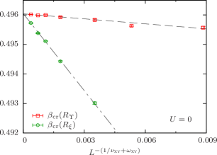
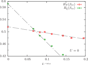
Figure 7: (Top) Crossing points $\beta_{\rm cr}(R_{\Upsilon};L,2L)$ and $\beta_{\rm cr}(R_{\xi};L,2L)$ for $U=0$ and $\mu=0$. They are plotted versus $L^{-1/{\nu_{\textsc{xy}}}-{\omega_{\textsc{xy}}}}=L^{-2.27}$, which is the expected behavior of the leading scaling corrections. The dashed lines correspond to linear fits of the data for the largest available lattices. (Bottom) Estimates of $R_{\Upsilon}$ and $R_{\xi}$ at the crossing points, versus $L^{-{\omega_{\textsc{xy}}}}=L^{-0.785}$. The dashed lines correspond to linear fits to $R^{*}+cL^{-{\omega_{\textsc{xy}}}}$ with $R^{*}$ fixed to its 3D XY value [$R_{\Upsilon}^{*}=0.516(1)$ and $R_{\xi}^{*}=0.5924(4)$], which is reported along the ordinate axis (crosses).

To begin with, we consider the hard-core 2BH model for $U=0$, representing two decoupled and identical single-component hard-core BH models. The results will then be compared with those obtained for $U\neq 0$.

In this case we have a robust theoretical prediction for its critical behavior at the BEC transition: it belongs to the 3D XY universality class, described by a standard U(1)-symmetric $\Phi^{4}$ theory with one complex order parameter. CN-14 ; CTV-13 ; PV-02 The leading scaling corrections decay with exponent $\omega_{1}={\omega_{\textsc{xy}}}=0.785(20)$, and the asymptotic critical values of $R_{\Upsilon}$ and $R_{\xi}$ are $R_{\Upsilon}^{*}=0.516(1)$ and $R_{\xi}^{*}=0.5924(4)$, respectively. CHPV-06 Numerical evidence of this critical behavior has already been reported in Refs. CTV-13, ; CN-14, .

We determine the crossing points footnote_cr $\beta_{\rm cr}(R;L,2L)$ for $L$ up to 32. Results are shown in the top panel of Fig. 7. The behavior for $L\to\infty$ is consistent with the expected $O(L^{-1/{\nu_{\textsc{xy}}}-{\omega_{\textsc{xy}}}})$ scaling corrections. Linear fits of the data for $L\gtrsim 20$ give $\beta_{c}=0.496035(10)$, footnote_betac which is in agreement with, and slightly improves, earlier estimates.CN-14 The values of $R_{\Upsilon}$ and $R_{\xi}$ at the crossing points are reported in the lower panel of Fig. 7. They show the expected asymptotic behavior $R(\beta_{\rm cr},L)=R^{*}+cL^{-{\omega_{\textsc{xy}}}}$. Moreover, the extrapolated values are consistent with the best available estimates for the 3D XY universality class. For example, linear fits of the data for $L\gtrsim 20$ give $R_{\Upsilon}^{*}=0.516(4)$, which is in agreement with the best available estimate CHPV-06 $R_{\Upsilon}^{*}=0.516(1)$ of the 3D XY universality class.

IV.3 QMC results for $U\not=0$

We now present results for the hard-core 2BH model for $U\not=0$. In this case we should consider the slowly-decaying scaling corrections of order $L^{-\omega_{u}}$ predicted in Sec. II.1, which are expected to give rise to significant systematic deviations, at least for negative $U$. Since $\omega_{u}=-0.0225$, these deviations are hardly detectable numerically. Indeed, in our range of values of $L$, $8\leq L\leq 64$, $L^{-\omega_{u}}$ varies only by 5%, hence it is very difficult to distinguish it from a constant term. In practice, unless data are extremely precise, any FSS analysis is unable to determine the leading scaling function $f_{R}(\tau L^{1/\nu})$ appearing in Eq. (19). The extrapolation of the data to $L\to\infty$ would identify the asymptotic behavior with that given by

$$\widetilde{f}_{R}(\tau L^{1/\nu})=f_{R}(\tau L^{1/\nu})+A\,g_{R}(\tau L^{1/\nu}),$$ (22)

where the slowing-decaying factor $L^{-\omega_{u}}$ is effectively replaced with some kind of average $A\equiv[L^{-\omega_{u}}]_{\rm av}$ in the considered range of values of $L$. This observation suggests that the analysis based on the large-$L$ extrapolation of the crossing points should be able to determine correctly $\beta_{c}$ and $\nu$. On the other hand, the extrapolation of the data for $R_{\Upsilon}$ and $R_{\xi}$ at the critical point would give $\widetilde{f}_{R}(0)$, which differs from the correct asymptotic estimate. In other words, we cannot rely on the values of the RG invariant quantities at the critical point to identify the universality class. In this discussion we have assumed that there is only a single slowly-decaying correction term, i.e., $L^{-\omega_{u}}$, which is, however, not the case. RG also predicts the presence of correction terms proportional to $L^{-n\omega_{u}}$ for any integer $n$, cf. Eq. (21), which makes the analysis of the corrections even more difficult. Finally, note that corrections of order $L^{-{\omega_{\textsc{xy}}}}$, the leading ones in the single-species model, are also expected.

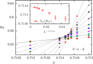
Figure 8: QMC estimates of $R_{\Upsilon}$ for $U=-5$ and $\mu=0$. The inset shows the crossing points $\beta_{\rm cr}(R_{\Upsilon};L,2L)$ versus $L^{-1/{\nu_{\textsc{xy}}}}$.

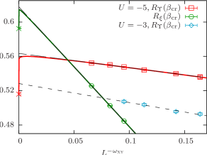
Figure 9: $R_{\Upsilon}$ and $R_{\xi}$ at the crossing points obtained using data for lattices of sizes $L$ and $2L$. Here $\mu=0$, $U=-5$ and $U=-3$. The straight lines correspond to linear fits to $R_{\#}(\beta_{\rm cr},L)=R_{\#}^{*}+cL^{-{\omega_{\textsc{xy}}}}$ with $R_{\#}^{*}$ and $c$ as free parameters (for $U=-5$ we obtain $R_{\Upsilon}(\beta_{\rm cr},L)=0.563-0.17L^{-{\omega_{\textsc{xy}}}}$ for $L\geq 12$ and $R_{\xi}(\beta_{\rm cr},L)=0.618-1.40L^{-{\omega_{\textsc{xy}}}}$ for $L\geq 20$). We also report the results of the fits to $R_{\#}(\beta_{\rm cr},L)=R_{\#}^{*}+c_{u}L^{-\omega_{u}}+cL^{-{\omega_{\textsc{xy}}}}$, in which $R_{\#}^{*}$ is fixed to the 3D XY critical value and $c_{u}$ and $c$ are free parameters (we obtain $R_{\Upsilon}(\beta_{\rm cr},L)=0.516+0.052L^{-{\omega_{u}}}-0.18L^{-{\omega_{\textsc{xy}}}}$ and $R_{\xi}(\beta_{\rm cr},L)=0.5924+0.028L^{-{\omega_{u}}}-1.41L^{-{\omega_{\textsc{xy}}}}$ for $U=-5$). The crosses on the vertical axis mark the best estimates of $R^{*}$ for the 3D universality class.

We first consider the attractive hard-core model with $U=-5$ and $\mu=0$. Fig. 8 reports the estimates of $R_{\Upsilon}$ as a function of $\beta$, which clearly show crossing points between $\beta=0.714$ and $\beta=0.715$. The crossing points $\beta_{\rm cr}(R_{\Upsilon};L,2L)$ up to $L=32$ are shown in the inset. We stress that their determination requires no prior knowledge on the nature of the transition, and it is therefore completely unbiased. They clearly appear to converge to a critical value $\beta_{c}$. The precision of the data does not allow us to distinguish the expected $O(L^{-1/{\nu_{\textsc{xy}}}-\omega_{u}})$ approach to the asymptotic value, as predicted by theory, from the $O(L^{-1/{\nu_{\textsc{xy}}}-{\omega_{\textsc{xy}}}})$ approach at $U=0$. Nevertheless, we obtain a reasonably precise estimate $\beta_{c}=0.7144(1)$, where the error also accommodates the difference of the extrapolations using the two ansatzes. Analogous results, although less precise, are obtained from the $R_{\xi}$ data.

The values of $R_{\Upsilon}$ and $R_{\xi}$ at the crossing points are shown in Fig. 9. They show an apparently linear behavior when plotted against $L^{-{\omega_{\textsc{xy}}}}$, as in the $U=0$ case. However, an extrapolation using the ansatze $R^{*}+cL^{-{\omega_{\textsc{xy}}}}$, which appears consistent with the data, gives critical values for $R_{\Upsilon}^{*}$ and $R_{\xi}^{*}$ which are definitely different from those of the 3D XY universality class. For example, we obtain $R_{\Upsilon}^{*}=0.563(2)$ and $R_{\xi}^{*}=0.625(5)$ with an acceptable $\chi^{2}/{\rm DOF}$ (DOF is the number of degrees of freedom of the fit), which differ significantly from the XY estimates $R_{\Upsilon}^{*}=0.516(1)$ and $R_{\xi}^{*}=0.5924(4)$. In view of the previous discussion, this discrepancy should be expected, because of the presence of the slowly-decaying $O(L^{-{\omega_{u}}})$ corrections with ${\omega_{u}}=0.0225(4)$. For instance, the data in Fig. 9 can also be nicely fitted to

$$R(\beta_{\rm cr})=R^{*}+aL^{-{\omega_{u}}}+bL^{-{\omega_{\textsc{xy}}}},$$ (23)

with $R^{*}$ fixed to its XY value, as shown in Fig. 9. Note that fits which include the $O(L^{-{\omega_{u}}})$ corrections are hardly distinguishable from the ones that assume the leading correction to be $L^{-{\omega_{\textsc{xy}}}}$ in the range of $L$ for which the MC data are available. This confirms that disentangling the correction term from the leading constant is extremely hard, requiring accurate computations for very large lattice sizes. It should be stressed that the fit to the ansatze (23) is only an exercise. It is presented to make plausible that the transition is in the XY universality class, even though a naive fit of the data provides a different value for $R^{*}$. Indeed, fit (23) is not conceptually correct unless $L$ is enormously large. RG predicts corrections of order $L^{-n{\omega_{u}}}$ for any integer $n$, that are as relevant as the leading one in our range of values of $L$.

To further check the above-reported results, we repeat the FSS analysis at fixed $\beta=0.7144$, varying the on-site coupling $U$ which now takes the role that $\beta$ had in the previous analysis. An analogous FSS analysis of data up to $L=48$ gives $U_{c}=-4.9999(3)$, which is perfectly consistent with the FSS analysis at fixed $U$. Moreover, the values of $R_{\Upsilon}$ and $R_{\xi}$ at the crossing points in the variable $U$ are hardly distinguishable from those appearing in Fig. 9 at the corresponding values of $L$.

We have also performed a FSS analysis of data for $U=-3$, up to $L=40$, obtaining $\beta_{c}=0.5390(2)$. The data of $R_{\Upsilon}$ at the crossing points $\beta_{\rm cr}(R_{\Upsilon};L,2L)$ are also shown in Fig. 9. As for $U=-5$, they appear to behave linearly with respect to $L^{-{\omega_{\textsc{xy}}}}$, and again they extrapolate to a value that is significantly larger than $R_{\Upsilon}^{*}\approx 0.516$. Such a deviation is smaller than that obtained for $U=-5$, confirming that the discrepancies cannot be interpreted as due to the presence of a new universality class. In that case, indeed, one would obtain the same extrapolated value for both values of $U$. Instead, the results are consistent with our RG predictions: the discrepancies increase with $|U|$, which is exactly what should be expected if they are related to the slowly-decaying corrections due to the interspecies interaction.

We finally mention that, as already anticipated in Sec. II.1, the scaling corrections induced by the density-density on-site interaction turn out to be small when the interspecies interaction is repulsive, that is for $U>0$. We have considered two values of $U$, $U=1$ and 10, and lattices up to $L=40$. In both cases, we obtain results for $R^{*}_{\Upsilon}$ and $R^{*}_{\xi}$ that are in agreement with the XY values. Apparently, the slowly-decaying corrections are negligible, being at most of the size of the statistical errors. Note that these corrections vanish for $U=0$ (the two models are decoupled) and also for $U\to+\infty$ (the model is equivalent to the hard-core BH model for a single boson, hence it has a standard XY transition without the $L^{-{\omega_{u}}}$ scaling corrections). Apparently, they keep on being small for all intermediate values of $U$.

IV.4 Phase diagram of the hard-core 2BH model at $\mu=0$

We determine the $U$ dependence of the normal-to-superfluid transition line by repeating the FSS analysis for other values of $U$. This is done with less accuracy, using data up to $L=24$. The results are shown in Fig. 10. The phase diagram is quite similar to that obtained in the mean-field approximation. In particular, the low-temperature superfluid phase disappears for $U\lesssim-6$, very close to the mean-field result $U=-6$. Indeed, as shown by the zero-temperature mean-field phase diagram shown in Figs. 4 and 5, $U=-6$ is the location of the quantum transition between the superfluid and $n=2$ Mott phase.

Finally, we discuss the behavior of the particle densities $n_{s}\equiv\langle n_{s\bm{x}}\rangle$ at the BEC transition. Their leading behavior at the BEC transitions arises from the analytical background terms, while the universal power laws related to the critical behavior are subleading. Indeed, standard RG arguments predict the asymptotic behavior

$$n_{s}\approx f_{a}(\tau)+L^{-y_{n}}f_{s}(\tau L^{1/\nu})$$ (24)

when varying the reduced temperature $\tau=1-\beta/\beta_{c}$ keeping fixed the model parameters. In Eq. (24), $f_{a}$ is a nonuniversal analytic function; $y_{n}$ is the RG dimension of the particle density operator $n_{s\bm{x}}$, which is given by $y_{n}=3-1/\nu=1.5112(2)$ at the decoupled XY FP; $f_{s}$ is a universal function apart from a factor and a rescaling of its argument. Therefore, the critical densities at $T_{c}$ are expected to approach a nonuniversal constant in the large-$L$ limit. In Fig. 11 we show the large-$L$ extrapolations of the particle-density data at $T_{c}$ versus the on-site coupling $U$. The comparison with the mean-field computations of Sec. III shows that the mean-field approximation of the particle density is quite accurate.

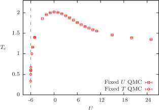
Figure 10: Transition line of the hard-core 2BH model for $\mu=0$, as obtained by the FSS analysis of QMC data. We plot $T_{c}\equiv 1/\beta_{c}$ versus $U$. Most estimates are obtained in simulations at fixed $U$ in which $T$ is varied. Close to $U=-6$, where the transition line is almost parallel to the $T$ axis, we performed simulations at fixed temperature, determining the critical coupling $U_{c}$.

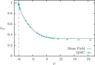
Figure 11: The single-species particle density $n_{s}\equiv\langle n_{s{\bm{x}}}\rangle$ along the critical line, as obtained by QMC and mean-field calculations.

V Conclusions

We investigate BEC in 3D two-component bosonic systems. In particular we consider two interacting identical bosonic gases, described by the 2BH model (I), which may be interpreted as a lattice two-component bosonic system. We study the phase diagram and the critical behavior by RG, mean-field, and numerical methods.

Our RG analysis is based on a LGW theory with two complex scalar fields (associated with the two bosonic components), which has the same symmetry as that of the bosonic system. In the case of two identical components with density-density interactions, the relevant global symmetry is ${\mathbb{Z}}_{2,e}\otimes{\rm U}(1)\otimes{\rm U}(1)$. The mean-field analysis predicts two different types of low-temperature phases. Depending on the values of the on-site inter-species $U$ and intra-species $V$ couplings, one may have (i) a phase in which the exchange symmetry is conserved and both components condense or (ii) a phase in which only one component condenses, thus breaking the ${\mathbb{Z}}_{2,e}$ exchange symmetry.

In case (i), which is generically expected for $V\gtrsim U$, the transition belongs to the 3D XY universality class. More precisely, the critical behavior is controlled by a decoupled XY FP, implying an asymptotic decoupling of the critical modes associated with the bosonic components. The density-density interaction between these two components turns out to be an irrelevant perturbation at this FP. It does not affect the asymptotic behavior but gives rise to slowly-decaying scaling corrections, that behave as $\xi^{-\omega_{u}}$, where $\xi$ is the diverging length scale at transition and $\omega_{u}=3-2/{\nu_{\textsc{xy}}}=0.0225(4)$. Of course, these slowly-decaying effects are absent at the transition of a single bosonic species, CN-14 ; CTV-13 ; CR-12 ; CPS-07 where the leading scaling corrections decay as $\xi^{-{\omega_{\textsc{xy}}}}$ with ${\omega_{\textsc{xy}}}\approx 0.78$. The presence of slowly decaying corrections makes an accurate check of the asymptotic 3D XY critical behavior quite hard, essentially because one needs to get very close to the critical point to make them negligible. These predictions are supported by a FSS analysis of QMC data for the 2BH model (I) in the hard-core limit, i.e., for $V\to\infty$.

The FT RG analysis predicts that the nature of the transition should significantly change in the soft-core regime, i.e. when $V\lesssim U$. In this case only one component is expected to condense. The corresponding symmetry breaking is therefore different, hence it leads to a different universality class in the case of continuous transitions. We identify this universality class with that of the chiral transition in frustrated two-component spin models with noncollinear order, Kawamura-88 ; PRV-01 ; CPPV-04 which has $\nu\approx 0.6$ as correlation-length exponent.

Our RG study also predicts the possibility of a critical behavior with an extended O(4) symmetry. However, such symmetry enlargement can only be observed by tuning a further parameter beside the temperature.

It should be stressed that the different critical behaviors can only be observed if the system is in the attraction domain of one of the FPs. If this is not the case, the transition would be of first order.

We also extend our analysis to the more general case in which the two bosonic components are not identical. The phase diagrams are expected to be more complex, as shown in Fig. 3. In particular, they may or may not show a low-temperature mixed phase characterized by the condensation of both components. According to mean-field and RG results, if the mixed phase is present, the phase diagram presents a tetracritical point where four transition lines meet, and the multicritical behavior is controlled by the decoupled XY FP. When the mixed phase is absent, thus the low-temperature phases are characterized by the BEC of only one component, the transitions between the two BEC phases must be first order. In this case the competition of the two U(1) orderings does not lead to a multicritical behavior, since no stable FPs are found in the corresponding parameter region; as a consequence the behavior at the intersection of the transition lines is expected to show thermodynamic discontinuities analogous to first-order transitions.

The RG analysis of BEC transitions in mixtures of bosonic gases can be straightforwardly extended to the two-dimensional (2D) case. In two dimensions bosonic systems do not experience BEC. The low-temperature phase of single species is characterized by a quasi-long range order, where correlations decay algebraically at large distances, without the emergence of a nonvanishing order parameter. The transitions to this low-temperature phase are generally of the Berezinskii-Kosterlitz-Thouless (BKT) type, Berezinski-72 ; KT-73 ; Kosterlitz-74 characterized by an exponential increase of the correlation length. The phase diagram of mixtures of 2D bosonic systems may show BKT transitions such as those of single bosonic species, and transitions related to the breaking of the $\mathbb{Z}_{2}$ exchange symmetry. A similar situation arises in 2D frustrated two-component spin models, see, e.g., Ref. HPV-05, , and references therein. RG scaling arguments analogous to those used for the 3D case allow us to infer that the critical behavior of identical interacting hard-core bosonic components is again controlled by a decoupled BKT FP. Since the energy operator is marginal at the BKT transition, i.e. $y_{e}=0$, the RG dimension of the density-density inter-species coupling is given by $y_{u}=2y_{e}-d=-2$ ($d=2$ in this case). Therefore, energy-energy or density-density interactions between the bosonic species are irrelevant also in two dimensions. Unlike the 3D case, the corresponding contributions get rapidly suppressed when approaching the critical point, indeed they are $O(\xi^{-2})$. Therefore, we expect that 2D identical hard-core bosonic components, such as the hard-core 2BH model (I) in two dimensions, undergo continuous transitions characterized by decoupled BKT behaviors with multiplicative and subleading logarithmic corrections,AGG-80 ; PV-13 analogous to the case of a single bosonic species CNPV-13 .

We finally note that cold-atom experiments are usually performed in inhomogeneous conditions, due to the presence of space-dependent trapping forces which effectively confine the atomic gas within a limited space region. CW-02 ; Ketterle-02 ; BDZ-08 The trapping potential is effectively coupled to the particle density. Thus, it can be taken into account by adding a space-dependent trap term such as

$$H_{\rm trap}=\sum_{\bm{x}}V_{t}({\bm{x}})n_{s\bm{x}},$$ (25)

to the BH Hamiltonian (I), where $V_{t}$ is the space-dependent potential associated with the external force. For example, we may consider $V_{t}(r)=(r/\ell_{t})^{2}$, where $r\equiv|{\bm{x}}|$ is the distance from the center ${\bm{x}}=0$ of the trap, which describes a harmonic rotationally-invariant trap. The inhomogeneity arising from the trapping potential introduces an additional length scale $\ell_{t}$ into the problem, which drastically changes the general features of the behavior at a phase transition. For example, the correlation functions of the critical modes do not develop a diverging length scale in a finite trap. Nevertheless, when the trap size $\ell_{t}$ becomes large, we may still observe a critical regime around the transition point, with universal trap-size scaling (TSS) behaviors with respect to the trap size $\ell_{t}$. TSS is controlled by the universality class of the phase transition of the homogeneous system. It has some analogies with the standard FSS for homogeneous systems which we exploited in our numerical study, see Sec. IV. The main difference is that, at the critical point, the correlation length $\xi$ around the center of the trap shows a nontrivial power-law dependence on the trap size $\ell_{t}$, i.e., $\xi\sim\ell_{t}^{\theta}$ where $\theta$ is the universal trap exponent. TSS has been numerically checked at the BEC transition of a single 3D bosonic gas.CTV-13 ; CN-14 Analogous TSS arguments can be applied to the BEC transitions of two-component bosonic gases. In particular, the trap exponent in the case of the harmonic space-dependence of $V_{t}$ turns out to be CV-09

$$\theta={2\nu\over 1+2\nu},$$ (26)

where $\nu$ is the correlation-length exponent of the transition, thus $\theta=0.57327(4)$ at the decoupled XY fixed point controlling the simultaneous condensation of both components, and $\theta\approx 0.5$ when only one component condenses.

Our study is relevant to experiments in which a mixture of two bosonic atomic vapours is cooled to the point that at least one of them undergoes a BEC transition and the number of particles is separately conserved between the two species. Recent years have seen the development of many such experiments, with the two bosonic species being two hyperfine levels of a single isotope PhysRevLett.78.586 ; PhysRevLett.81.1539 ; PhysRevLett.82.2228 ; PhysRevLett.99.190402 ; PhysRevLett.103.245301 ; PhysRevLett.105.045303 ; PhysRevA.82.033609 ; PhysRevLett.85.2413 ; PhysRevA.63.051602 ; PhysRevA.80.023603 , two isotopes of the same element PhysRevLett.101.040402 ; PhysRevA.84.011610 ; PhysRevA.79.021601 or heteronuclear mixtures of different elements PhysRevLett.89.053202 ; PhysRevLett.89.190404 ; PhysRevLett.99.010403 ; PhysRevA.77.011603 ; PhysRevLett.100.210402 . Notably, some mixtures were also successfully loaded on optical lattices PhysRevLett.105.045303 ; PhysRevA.77.011603 ; PhysRevLett.100.210402 . The availability of a wide range of atomic species and the presence of Fano-Feshbach resonances allow to tune the intra-species and inter-species interactions between the two components of the mixtures. Additional control can be achieved by acting on the depth of an optical lattice. The high degree of tunability of these systems may make the direct observation of the transitions we predict within the reach of experiments.

- (1) E.A. Cornell and C.E. Wieman, Nobel Lecture: Bose-Einstein condensation in a dilute gas, the first 70 years and some recent experiments, Rev. Mod. Phys. 74, 875 (2002).
- (2) N. Ketterle, Nobel lecture: When atoms behave as waves: Bose-Einstein condensation and the atom laser, Rev. Mod. Phys. 74, 1131 (2002).
- (3) I. Bloch, J. Dalibard, and W. Zwerger, Many-body physics with ultracold gases, Rev. Mod. Phys. 80, 885 (2008).
- (4) J.A. Lipa, D.R. Swanson, J.A. Nissen, T.C.P. Chui, and U.E. Israelsson, Heat Capacity and Thermal Relaxation of Bulk Helium very near the Lambda Point, Phys. Rev. Lett. 76, 944 (1996).
- (5) M. Campostrini, M. Hasenbusch, A. Pelissetto, and E. Vicari, Theoretical estimates of the critical exponents of the superfluid transition in 4He by lattice methods, Phys. Rev. B 74, 144506 (2006).
- (6) A. Pelissetto and E. Vicari, Critical phenomena and renormalization-group theory, Phys. Rep. 368, 549 (2002).
- (7) T. Donner, S. Ritter, T. Bourdel, A. Öttl, M. Köhl, and T. Esslinger, Critical Behavior of a Trapped Interacting Bose Gas, Science 315, 1556 (2007).
- (8) C. J. Myatt, E. A. Burt, R. W. Ghrist, E. A. Cornell and C. E. Wieman, Production of Two Overlapping Bose-Einstein Condensates by Sympathetic Cooling, Phys. Rev. Lett. 78, 586 (1997).
- (9) D. S. Hall, M. R. Matthews, J. R. Ensher, C. E. Wieman and E. A. Cornell, Dynamics of Component Separation in a Binary Mixture of Bose-Einstein Condensates, Phys. Rev. Lett. 81, 1539 (1998).
- (10) H. Miesner, D. M. Stamper-Kurn, J. Stenger, S. Inouye, A. P. Chikkatur and W. Ketterle, Observation of Metastable States in Spinor Bose-Einstein Condensates, Phys. Rev. Lett. 82, 2228 (1999).
- (11) G. Delannoy, S. G. Murdoch, V. Boyer, V. Josse, P. Bouyer and A. Aspect, Understanding the production of dual Bose-Einstein condensation with sympathetic cooling, Phys. Rev. A 63, 051602 (2001).
- (12) K. M. Mertes, J. W. Merrill, R. Carretero-González, D. J. Frantzeskakis, P. G. Kevrekidis and D. S. Hall, Nonequilibrium Dynamics and Superfluid Ring Excitations in Binary Bose-Einstein Condensates, Phys. Rev. Lett. 99, 190402 (2007).
- (13) D. M. Weld, P. Medley, H. Miyake, D. Hucul, D. E. Pritchard and W. Ketterle, Spin Gradient Thermometry for Ultracold Atoms in Optical Lattices, Phys. Rev. Lett. 103, 245301 (2009).
- (14) R. P. Anderson, C. Ticknor, A. I. Sidorov and B. V. Hall, Spatially inhomogeneous phase evolution of a two-component Bose-Einstein condensate, Phys. Rev. A 80, 023603 (2009).
- (15) B. Gadway, D. Pertot, R. Reimann and D. Schneble, Superfluidity of Interacting Bosonic Mixtures in Optical Lattices, Phys. Rev. Lett. 105, 045303 (2010).
- (16) S. Tojo, Y. Taguchi, Y. Masuyama, T. Hayashi, H. Saito and T. Hirano, Controlling phase separation of binary Bose-Einstein condensates via mixed-spin-channel Feshbach resonance, Phys. Rev. A 82, 033609 (2010).
- (17) J. Stenger, S. Inouye, D. M. Stamper-Kurn, H.-J. Miesner, A. P. Chikkatur and W. Ketterle, Spin domains in ground-state Bose-Einstein condensates, Nature 396, 345 (1998).
- (18) P. Maddaloni, M. Modugno, C. Fort, F. Minardi and M. Inguscio, Collective Oscillations of Two Colliding Bose-Einstein Condensates, Phys. Rev. Lett. 85, 2413 (2000).
- (19) G. Ferrari, M. Inguscio, W. Jastrzebski, G. Modugno, G. Roati and A. Simoni, Collisional Properties of Ultracold K-Rb Mixtures, Phys. Rev. Lett. 89, 053202 (2002).
- (20) G. Modugno, M. Modugno, F. Riboli, G. Roati and M. Inguscio, Two Atomic Species Superfluid, Phys. Rev. Lett. 89, 190404 (2002).
- (21) G. Roati, M. Zaccanti, C. D’Errico, J. Catani, M. Modugno, A. Simoni, M. Inguscio and G. Modugno, Bose-Einstein Condensate with Tunable Interactions, Phys. Rev. Lett. 99, 010403 (2007).
- (22) J. Catani, L. De Sarlo, G. Barontini, F. Minardi and M. Inguscio, Degenerate Bose-Bose mixture in a three-dimensional optical lattice, Phys. Rev. A 77, 011603 (2008).
- (23) G. Thalhammer, G. Barontini, L. De Sarlo, J. Catani, F. Minardi and M. Inguscio, Double Species Bose-Einstein Condensate with Tunable Interspecies Interactions, Phys. Rev. Lett. 100, 210402 (2008).
- (24) S. B. Papp, J. M. Pino and C. E. Wieman, Tunable Miscibility in a Dual-Species Bose-Einstein Condensate, Phys. Rev. Lett. 101, 040402 (2008).
- (25) T. Fukuhara, S. Sugawa, Y. Takasu and Y. Takahashi, All-optical formation of quantum degenerate mixtures, Phys. Rev. A 79, 021601 (2009).
- (26) S. Sugawa, R. Yamazaki, S. Taie and Y. Takahashi, Bose-Einstein condensate in gases of rare atomic species, Phys. Rev. A 84, 011610 (2011).
- (27) T.-L. Ho and V.B. Shenoy, Binary mixtures of Bose condensates of alkali atoms, Phys. Rev. Lett. 77, 3276 (1996).
- (28) M. Boninsegni, Phase separation in mixtures of hard-core bosons, Phys. Rev. Lett. 87, 087201 (2001).
- (29) E. Altman, W. Hofstetter, E. Demler, and M.D. Lukin, Phase diagram of two-component bosons on an optical lattice, New J. Phys. 5, 113 (2005).
- (30) L.-M. Duan, E. Demler, and M.D. Lukin, Controlling spin exchange interactions of ultracold atoms in optical lattices, Phys. Rev. Lett. 91, 090402 (2003).
- (31) A.B. Kuklov and B.V. Svistunov, Counterflow superfluidity of two-species ultracold atoms in a commensurate optical lattice, Phys. Rev. Lett. 90, 100401 (2003).
- (32) B. Paredes and J.I. Cirac, From Cooper pairs to Luttinger liquids with Bosonic atoms in optical lattices, Phys. Rev. Lett. 90, 150402 (2003).
- (33) K.V. Krutitsky and R. Graham, Spin-1 bosons with coupled ground states in optical lattices, Phys. Rev. A 70, 063610 (2004).
- (34) A.B. Kuklov, N. Prokof’ev, and B.V. Svistunov, Superfluid-superfluid phase transitions in a two-component Bose-Einstein condensate, Phys. Rev. Lett. 92, 030403 (2004).
- (35) A. Isacsson, M.-C. Cha, K. Sengupta, and S.M. Girvin, Superfluid-insulator transitions of two-species bosons in an optical lattice, Phys. Rev. B 72, 184507 (2005).
- (36) R.V. Pai, K. Sheshadri and R. Pandit, Phases and transitions in the spin-1 Bose-Hubbard model: Systematics of a mean-field theory, Phys. Rev. B 77, 014503 (2008).
- (37) S.G. Söyler, B. Capogrosso-Sansone, N.V. Prokof’ev, and B.V. Svistunov, Sign-alternating interaction mediated by strongly correlated lattice bosons, New. J. Phys. 11, 073036 (2009).
- (38) A. Hubener, M. Snoek and W. Hofstetter, Magnetic phases of two-component ultracold bosons in an optical lattice, Phys. Rev. B 80, 245109 (2009).
- (39) B. Capogrosso-Sansone, S.G. Söyler, N.V. Prokof’ev, and B.V. Svistunov, Critical entropies for magnetic ordering in bosonic mixtures on a lattice, Phys. Rev. A 81, 053622 (2010).
- (40) L. de Forges de Parny, F. Hébert, V.G. Rousseau, R.T. Scalettar, and G.G. Batrouni, Ground state phase diagram of spin-1/2 bosons in a two-dimensional optical lattice, Phys. Rev. B 84, 064529 (2011).
- (41) L. Pollet, Recent developments in Quantum Monte-Carlo simulations with applications for cold gases, Rep. Prog. Phys. 75, 094501 (2012).
- (42) A. Angelone, M. Campostrini, and E. Vicari, Universal quantum behaviors of interacting fermions in 1D traps: from few particles to the trap thermodynamic limit, Phys. Rev. A 89, 023635 (2014).
- (43) J.-P. Lv, Q.-H. Chen, and Y. Deng, Two-species hard-core bosons on the triangular lattice: A quantum Monte Carlo study, Phys. Rev. A 89, 013628 (2014).
- (44) P.N. Galteland, E. Babaev, and A. Sudbø, Immiscibile two-component Bose Einstein condensates beyond mean-field approximation: phase transitions and rotational response, arXiv:1503.05583.
- (45) G. Ceccarelli and J. Nespolo, Universal scaling of three-dimensional bosonic gases in a trapping potential, Phys. Rev. B 89, 054504 (2014).
- (46) G. Ceccarelli, C. Torrero, and E. Vicari, Critical parameters from trap-size scaling in trapped particle systems, Phys. Rev. B 87, 024513 (2013).
- (47) J. Carrasquilla and M. Rigol, Superfluid to normal phase transition in strongly correlated bosons in two and three dimensions, Phys. Rev. A 86, 043629 (2012).
- (48) B. Capogrosso-Sansone, N.V. Prokof’ev, and B.V. Svistunov, Phase diagram and thermodynamics of the three-dimensional Bose-Hubbard model, Phys. Rev. B 75, 134302 (2007).
- (49) H. Kawamura, Renormalization-group analysis of chiral transitions, Phys. Rev. B 38, 4916 (1988).
- (50) A. Aharony, Dependence of universal critical behaviour on symmetry and range of interaction. – In: Phase Transitions and Critical Phenomena. Vol. 6, edited by C. Domb and M.S. Green, (Academic, New York, 1976) p. 357.
- (51) J. Zinn-Justin, Quantum Field Theory and Critical Phenomena, fourth edition (Clarendon Press, Oxford, 2002).
- (52) E. Vicari, Critical phenomena and renormalization-group flow of multi-parameter field theories, PoS (LAT2007) 023; arXiv:0709.1014.
- (53) A. Pelissetto and E. Vicari, Interacting -vector order parameters with O() symmetry, Condensed Matter Physics (Ukraine) 8, 87 (2005).
- (54) A. Pelissetto, P. Rossi, and E. Vicari, The critical behavior of frustrated spin models with noncollinear order, Phys. Rev. B 63, 140414(R) (2001).
- (55) P. Calabrese, P. Parruccini, A. Pelissetto, and E. Vicari, Critical behavior of O(2)O()-symmetric models, Phys. Rev. B 70, 174439 (2004).
- (56) The existence of the chiral FP in O()O(2) models for has been questioned in several papers. See, e.g., M. Tissier, B. Delamotte, and D. Mouhanna, XY frustrated systems: continuous exponents in discontinuous phase transitions, Phys. Rev. B 67, 134422 (2003), for alternative interpretations of the theoretical and experimental results. However, quite recently a chiral FP has been identified in the O(3)O(2) theory, using a completely different method, the so-called conformal bootstrap approach: see Y. Nakayama and T. Ohtsuki, Bootstrapping phase transitions in QCD and frustrated spin systems, Phys. Rev. D 91, 021901 (2015). These results (although they only apply to ) further support the existence of a chiral FP in these models.
- (57) M. Hasenbusch and E. Vicari, Anisotropic perturbations in three-dimensional O()-symmetric vector models, Phys. Rev. B 84, 125136 (2011).
- (58) M. Hasenbusch, Eliminating leading corrections to scaling in the three-dimensional -symmetric model: and 4, J. Phys. A 34, 8221 (2001).
- (59) P. Calabrese, A. Pelissetto, and E. Vicari, Multicritical behavior of -symmetric systems, Phys. Rev. B 67, 054505 (2003).
- (60) D. R. Nelson, J. M. Kosterlitz, and M.i E. Fisher, Renormalization-Group Analysis of Bicritical and Tetracritical Points, Phys. Rev. Lett. 33, 813 (1974).
- (61) J. M. Kosterlitz, D. R. Nelson, and M. E. Fisher, Bicritical and tetracritical points in anisotropic antiferromagnetic systems, Phys. Rev. B 13, 412 (1976).
- (62) A. Aharony, Comment on “Bicritical and Tetracritical Phenomena and Scaling Properties of the SO(5) Theory”, Phys. Rev. Lett. 88, 059703 (2002).
- (63) F. H. L. Essler, H. Frahm, F. Göhmann, A. Klümper, and V. E. Korepin, The One–Dimensional Hubbard Model (Cambridge University Press, Cambridge, 2005).
- (64) A. W. Sandvik and J. Kurlijärvi, Quantum Monte Carlo simulation method for spin systems, Phys. Rev. B 43, 5950 (1991).
- (65) O. F. Syljuåsen and A. W. Sandvik, Quantum Monte Carlo with directed loops, Phys. Rev. E 66, 046701 (2002).
- (66) A. Dorneich and M. Troyer, Accessing the dynamics of large many-particle systems using the stochastic series expansion, Phys. Rev. E 64, 066701 (2001).
- (67) Our implementation of the directed operator-loop SSE algorithm is a natural extension to the two-species hard-core BH model of the single species algorithm. There are 32 matrix elements, giving rise to possible transitions for each species. The operator loops always act on a single species at the time: at the beginning of each loop, we randomly select the species to update.
- (68) At fixed , for each , we interpolated the data in a neighborhood of the crossing point with a cubic polynomial (or with a quadratic one if not enough data points are available for a cubic regression). Subsequently, we numerically evaluated the crossing point between the interpolants, using bootstrap methods to estimate the error.
- (69) The fit is repeated, progressively discarding the data from the smaller lattice sizes, i.e., by only fitting the crossing points for which . This allows us to control residual corrections to scaling.
- (70) V. L. Berezinski, Destruction of long-range order in one-dimensional and 2-dimensional systems having a continuous symmetry group. 1. Classical systems, Sov. Phys. JETP 32, 493 (1971).
- (71) J. M. Kosterlitz and D. J. Thouless, Ordering, metastability and phase transitions in two-dimensional systems, J. Phys. C 6, 1181 (1973).
- (72) J. M. Kosterlitz, Critical properties of the 2-dimensional XY model, J. Phys. C 7, 1046 (1974).
- (73) M. Hasenbusch, A. Pelissetto, and E. Vicari, Multicritical behavior in the fully frustrated XY model and related systems, J. Stat. Mech. (2005) P12002.
- (74) D. J. Amit, Y. Y. Goldschmidt, and G. Grinstein, Renormalization group analysis of the phase transition in the 2D Coulomb gas, sine-Gordon theory and XY model, J. Phys. A 13, 585 (1980).
- (75) A. Pelissetto and E. Vicari, Renormalization-group flow and asymptotic behaviors at the Berezinskii-Kosterlitz-Thouless transitions, Phys. Rev. E 87, 032105 (2013).
- (76) G. Ceccarelli, J. Nespolo, A. Pelissetto, and E. Vicari, Universal behavior of two-dimensional bosonic gases at Berezinskii-Kosterlitz-Thouless transitions, Phys. Rev. B 88, 024517 (2013).
- (77) M. Campostrini and E. Vicari, Critical behavior and scaling in trapped systems, Phys. Rev. Lett. 102, 240601 (2009); (E) 103, 269901 (2009); Trap-size scaling in confined particle systems at quantum transitions, Phys. Rev. A 81, 023606 2010.