Stochastic approximation of dynamical exponent at quantum critical point

Abstract

We have developed a unified finite-size scaling method for quantum phase transitions that requires no prior knowledge of the dynamical exponent $z$. During a quantum Monte Carlo simulation, the temperature is automatically tuned by the Robbins-Monro stochastic approximation method, being proportional to the lowest gap of the finite-size system. The dynamical exponent is estimated in a straightforward way from the system-size dependence of the temperature. As a demonstration of our novel method, the two-dimensional $S=1/2$ quantum $XY$ model in uniform and staggered magnetic fields is investigated in the combination of the world-line quantum Monte Carlo worm algorithm. In the absence of the uniform magnetic field, we obtain the fully consistent result with the Lorentz invariance at the quantum critical point, $z=1$, i.e., the three-dimensional classical $XY$ universality class. Under a finite uniform magnetic field, on the other hand, the dynamical exponent becomes two, and the mean-field universality with effective dimension $(2+2)$ governs the quantum phase transition.

I Introduction

Recent enhancement of the computational power has enabled us to simulate larger-scale systems with higher precision than ever before. In particular, with the help of the recent development of simulation algorithms for strongly correlated quantum systems, a number of simulations have been performed to elucidate the novel nature of quantum phase transitions, in which many-body physics plays an essential role Sachdev (1999); Avella and Mancini (2013). Quantum phase transitions occur at absolute zero temperature, triggered by quantum fluctuations. Through the quantum-classical mapping, a quantum phase transition in $d$ dimensions, if it is of second order, can be generally described by the critical theory as the temperature-driven phase transition in a $(d+z)$-dimensional classical system with the same symmetries, where $z$ is the so-called dynamical exponent Suzuki (1976); Vojta (2003).

A world-line quantum Monte Carlo (WLQMC) method is one of the most powerful tools for investigating quantum critical phenomena without any bias or approximation Suzuki (1994); Landau and Binder (2005). A quantum system in $d$ dimensions is mapped to a classical system in $(d+1)$ dimensions in the WLQMC method. The system length along the additional direction, the imaginary-time direction, is given by the inverse temperature, $\beta$.

When one performs a WLQMC simulation to investigate quantum criticality, the choice of $\beta$ for each system size is essential. The reason is that the quantum critical system can be extremely anisotropic even if the interactions are isotropic in real space. While the correlation length in the real-space direction diverges as $\xi\sim(g-g_{\mathrm{c}})^{-\nu}$, that in the imaginary-time direction does as $\xi_{\tau}\sim(g-g_{\mathrm{c}})^{-z\nu}$, where $g$ is the coupling constant that controls quantum fluctuations, $g_{\mathrm{c}}$ the quantum critical point, and $\nu$ the critical exponent. If the dynamical exponent $z$ is one, the space-time isotropy is kept aside from a scale factor, or the velocity of low-energy excitation. In the meanwhile, there are phase transitions with a dynamical exponent larger than one. The Bose-Hubbard model with randomness that exhibits quantum criticality with $z>1$ has been extensively investigated analytically Fisher et al. (1989); Singh and Rokhsar (1992); Herbut (1997); Weichman and Mukhopadhyay (2007), numerically Sørensen et al. (1992); Zhang et al. (1995); Prokof’ev and Svistunov (2004); Priyadarshee et al. (2006); Meier and Wallin (2012); Álvarez Zúñiga et al. (2015) as well as experimentally Hüvonen et al. (2012); Yu et al. (2012).

Let us review the renormalization group and the scaling theory near a quantum critical point. Consider the scale transformation with a certain length scale, $b$. A physical quantity, denoted as $F$, is generally transformed as

$$\begin{split}F(g-g_{\mathrm{c}},L^{-1},\beta^{-1})&=b^{y_{F}}F(b^{1/\nu}(g-g_{\mathrm{c}}),bL^{-1},b^{z}\beta^{-1})\\ &=L^{y_{F}}\tilde{F}(L^{1/\nu}(g-g_{\mathrm{c}}),L^{z}\beta^{-1}),\end{split}$$ (1)

where $y_{F}$ is the scaling dimension of the quantity under consideration. In the second line of Eq. (1), we chose $b=L$ and introduced $\tilde{F}(x,y)\equiv F(x,1,y)$. This equation has several unknown constants, $g_{\mathrm{c}}$, $y_{F}$, $\nu$, $z$, and the scaling function $\tilde{F}(x,y)$ itself.

In order to determine the constants in the finite-size scaling ansatz (1), one had to repeat simulations densely in the three-dimensional parameter space $(L,\beta,g)$, and perform a multi-parameter finite-size scaling analysis as in Refs. 19 and 20. It typically requires considerable computational resources to scan the multi-dimensional parameter space. Instead of the exhaustive scanning, simulations with some assumed $z$ were performed in most previous studies. The consistency was checked after the calculation as in Ref. 21. This approach, however, would be awfully inefficient in the case without knowledge of the value of $z$ in advance. Another approach for $z$ estimation was to focus on the temperature dependence of the correlation length, $\xi\sim\beta^{1/z}$ at $g=g_{\mathrm{c}}$ and $L=\infty$ Priyadarshee et al. (2006). After the correlation length in the thermodynamic limit was extrapolated at each temperature, the low-temperature asymptotic behavior was analyzed. This two-step procedure requires additional computational cost, and possibly introduces some uncontrollable systematic error from the extrapolations, even if the location of quantum critical point, $g_{\mathrm{c}}$, is known. In the meantime, the winding numbers of the world-lines in space and time directions were exploited in Refs. 22 and 23. A parameter, $L$ or $\beta$, was interpolated so that the winding number squared in each direction averagely took the same value. However, such an interpolation is again non-trivial in a multi-parameter space and multi conditions.

Fig 1: (Color online) Schematic pictures of virtually (a) anisotropic and (b) isotropic systems, where $L$ and $\beta$ are the system linear length in the real space and the imaginary time directions, respectively. The blue oval in each picture depicts space-time region correlated with the center (red cross). After the aspect-ratio optimization, the relative correlation lengths, $\xi/L$ and $\xi_{\tau}/\beta$, become almost the same.

One of the most effective strategies to overcome the difficulty of a multi-parameter scaling is to introduce an auto-tuning technique. A number of auto-tuning techniques have already been used in numerical simulations in the field of statistical physics. For example, the invaded cluster algorithm Machta et al. (1995) or the probability-changing cluster algorithm Tomita and Okabe (2001) can automatically locate the critical point. The Wang-Landau algorithm Wang and Landau (2001) enables us to directly estimate the density of states of a system.

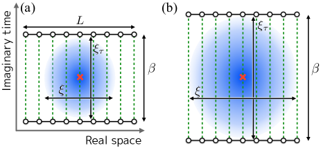
In the present paper, we employ the stochastic approximation method. Recently in Ref. 27, a method to automatically optimize the aspect ratio of a quantum system was proposed for analyzing quantum criticality under strong spatial anisotropy. The relative correlation length, $R_{\alpha}\equiv\xi_{\alpha}/L_{\alpha}$, where $\xi_{\alpha}$ and $L_{\alpha}$ are the correlation length and the system size in $\alpha$ direction, respectively ($\alpha=x$, $y$, or $\tau$ for two-dimensional systems and $L_{\tau}=\beta$), was adjusted for making the system virtually isotropic as $R_{x}:R_{y}:R_{\tau}\approx 1:1:1$. Figure 1 schematically illustrates virtually anisotropic and isotropic one-dimensional quantum systems. In Ref. 27, the stochastic approximation scheme was applied to the staggered dimer antiferromagnetic Heisenberg model, and the universality class of the quantum critical point was successfully identified in spite of the existence of strong finite-size corrections that easily lead a naive finite-size scaling analysis to an incorrect conclusion Wenzel and Janke (2009); Wenzel et al. (2008). Note that the tuning method using the correlation length Yasuda and Todo (2013) is applicable to general systems, while the method based on the winding number Jiang (2011, 2012) works only for systems with U(1) symmetry.

The aim of the present paper is to propose a unified finite-size scaling method based on the stochastic approximation technique for quantum criticality with general $z$. The relevant critical exponents including the dynamical exponent will be obtained simultaneously without any prior knowledge or assumption of the values. We will demonstrate our approach for the two-dimensional $S=1/2$ quantum $XY$ model in uniform and staggered magnetic fields along $z$ direction (in spin space). We will clarify that the dynamical exponent becomes two under a finite uniform magnetic field, while it does one in the absence of a uniform field.

This paper is organized as follows: Sec. II introduces the scaling ansatz of the correlation lengths for space-time anisotropic systems, the Robbins-Monro stochastic approximation method, and its convergence property. It is also discussed how the stochastic approximation method is applied to the present finite-size scaling analysis. In Sec. III, the model considered in the present paper and the WLQMC method are introduced. The numerical results are shown in Sec. IV. Finally our study is concluded in Sec. V. The technical details are reported in Appendices A and B.

II Stochastic approximation method

II.1 Conditions for realizing space-time isotropy

As noted in Sec. I, for the system with $z>1$, one should pay attention to the space-time aspect ratio when considering the finite-size scaling analysis. In this section, we explain conditions to realize a virtually isotropic system during a simulation. For simplicity, we assume that the model considered hereafter has no anisotropy in real space. Generalization to systems with spatial anisotropy is straightforward.

Let us start by choosing $F=\xi$ in Eq. (1). In this case, $y_{F}$ is one, i.e.,

$$\xi(g-g_{\mathrm{c}},L^{-1},\beta^{-1})=L\,\tilde{\xi}((g-g_{\mathrm{c}})L^{1/\nu},L^{z}/\beta).$$ (2)

Another choice, $F=\xi_{\tau}$, yields

$$\xi_{\tau}(g-g_{\mathrm{c}},L^{-1},\beta^{-1})=L^{y_{\tau}}\tilde{\xi_{\tau}}((g-g_{\mathrm{c}})L^{1/\nu},L^{z}/\beta),$$ (3)

where we set $y_{F}=y_{\tau}$. At the quantum critical point, $g=g_{\mathrm{c}}$, the correlation length in the imaginary-time direction exhibits the power law, $\xi_{\tau}(L^{-1})\propto L^{y_{\tau}}$, in the limit of $\beta\to\infty$. By the definition of the dynamical exponent, one finds $y_{\tau}=z$. Then, dividing both sides of Eq. (3) by $\beta$ yields

$$\xi_{\tau}(g-g_{\mathrm{c}},L^{-1},\beta^{-1})/\beta=\tilde{\xi}_{\tau}^{\prime}((g-g_{\mathrm{c}})L^{1/\nu},L^{z}/\beta),$$ (4)

where $\tilde{\xi}_{\tau}^{\prime}(x,y)\equiv y\,\tilde{\xi}_{\tau}(x,y)$.

Here, let us introduce two conditions,

$$\xi/L=R,$$ (5)

where $R$ is an arbitrarily chosen constant, and

$$\xi_{\tau}/\beta=R_{\tau},$$ (6)

where $R_{\tau}$ is another constant. Assume that conditions (5) and (6) are both satisfied by tuning $g$ and $\beta$ in simulating systems with different system sizes. If this is the case, $\tilde{\xi}$ and $\tilde{\xi}_{\tau}^{\prime}$ are kept constant even though they are different functions. Meanwhile, the set of arguments of $\tilde{\xi}$ in Eq. (2) and that of $\tilde{\xi}_{\tau}^{\prime}$ in Eq. (4) are the same as each other. That is, the different functions $\tilde{\xi}$ and $\tilde{\xi}_{\tau}^{\prime}$ sharing the same arguments are kept constant at different system sizes. This means that each of the arguments should be constant if the functions have some reasonable monotonicity. The monotonicity of the scaling functions is expected to hold near a generic critical point and supported by our numerical calculation shown below. Then Eqs. (5) and (6) provide solutions, $g_{\mathrm{c}}(L)$ and $\beta(L)$, for each system size:

$$g_{\mathrm{c}}(L)-g_{\mathrm{c}}\propto L^{-1/\nu}$$ (7)

and

$$\beta(L)\propto L^{z}.$$ (8)

Thus, the coupling constant, $g$, automatically converges to the critical point as $L$ increases. Moreover, the dynamical exponent can be simultaneously estimated from the asymptotic $L$ dependence of the inverse temperature, $\beta$.

II.2 Robbins-Monro stochastic approximation method

In this section, we introduce an iteration procedure to fulfill the conditions proposed in the previous section. Our task is to solve the system of nonlinear equations, $\xi/L=R$ and $\xi_{\tau}/\beta=R_{\tau}$, with respect to $g$ and $\beta$ for given $L$, $R$, and $R_{\tau}$. The solution cannot be obtained by standard iterative methods for nonlinear equations, such as the Newton-Raphson method. It is because $\xi$ and $\xi_{\tau}$ have statistical errors coming from the Monte Carlo sampling that make the conventional methods unstable. We thus employ the stochastic approximation method explained below.

Let us see a concrete example of the stochastic approximation. For simplicity, assume that $g$ is already set to $g_{\mathrm{c}}$. We estimate the optimal $\beta$ that satisfies the relation $\xi_{\tau}/\beta=R_{\tau}$. The solution of this equation is denoted as $\beta_{\mathrm{c}}$. First, one runs a short Monte Carlo simulation with a trial parameter $\beta^{(1)}$ and measures the correlation length, then calculates $A(\beta^{(1)})\equiv R_{\tau}-\xi_{\tau}/\beta^{(1)}$. Next, one updates the parameter, $\beta$, by using the Robbins-Monro type update procedure Robbins and Monro (1951); Bishop (2006)

$$\beta^{(n+1)}=\beta^{(n)}-\frac{p}{n}A(\beta^{(n)})$$ (9)

with $n=1$ and repeats the above until $\beta^{(n)}$ converges to a certain value with increasing $n=2,3,4,\cdots$. Here, $p$ is a (constant) parameter that determines the gain of the feedback. Regardless of the choice of the gain, it is proved that $\beta^{(n)}$ converges to $\beta_{\mathrm{c}}$ in $n\to\infty$ with probability one Robbins and Monro (1951); Albert and Gardner (1970).

As explained in Appendix A, the mean of the probability distribution of $\beta^{(n)}$ at the $n$-th step (denoted as $\mu_{n}$) converges as $\mu_{n}-\beta_{\mathrm{c}}\sim 1/n^{ap}$, where $a$ is the derivative of $A(\beta)$ at $\beta=\beta_{\mathrm{c}}$, and the sign of $p$ is chosen as the same with $a$. For $ap\leq 1/2$, the variance of $\beta^{(n)}$ at the $n$-th step (denoted as $\sigma_{n}^{2}$) is evaluated as $\sigma_{n}^{2}\sim 1/n^{2ap}$. For $ap>1/2$, on the other hand, $\sigma_{n}^{2}\sim s^{2}/n$, where $s^{2}\equiv\sigma^{2}p^{2}/(2ap-1)$ is the asymptotic variance and $\sigma$ is the statistical error resulting from a Monte Carlo estimation of $A(\beta)$. Here we should set $p\approx 1/a$ to minimize the variance (see the detailed discussion in Appendix A). By this choice of $p$, it is also guaranteed that the systematic error of $\beta^{(n)}$ decreases faster than the statistical (standard) error. In actual simulations, one needs to perform some ($\sim$10 at least) independent stochastic approximation processes to estimate error bars of $\beta$ and physical quantities. The number of steps of each approximation process has to be large enough ($\gtrsim 10^{2}$ typically) for the systematic error to become negligible in comparison to the statistical error.

The present stochastic approximation method can be extended to multi-dimensional problems in a straightforward way. Below, we will apply the method to the quantum phase transition of two-dimensional $S=1/2$ $XY$ model in uniform and staggered magnetic fields in order to demonstrate the efficiency of the present approach and clarify the quantum phase transitions.

III Model and quantum Monte Carlo method

III.1 $S=1/2$ quantum $XY$ model in uniform and staggered magnetic fields

The Hamiltonian of the two-dimensional $S=1/2$ quantum $XY$ model in uniform and staggered magnetic fields is defined as follows:

$$\mathcal{H}=-\frac{1}{2}\sum_{\langle j,k\rangle}(S_{j}^{+}S_{k}^{-}+S_{k}^{+}S_{j}^{-})-\sum_{j}\left[h^{\mathrm{u}}+h^{\mathrm{s}}(-1)^{\sigma(j)}\right]S_{j}^{z},$$ (10)

where $S_{j}^{+}$ ($S_{j}^{-}$) is the $S^{z}$-component raising (lowering) operator at site $j$, $\langle j,k\rangle$ denotes a pair of nearest-neighboring spins, and $h^{\mathrm{u}}$ ($h^{\mathrm{s}}$) is the amplitude of the uniform (staggered) magnetic field. Here we consider the square lattice of linear extent $L$ with the periodic boundary conditions, and the lattice is bipartite with even $L$. If site $j$ belongs to one of the sublattices, $\sigma(j)$ takes zero, otherwise $\sigma(j)=1$.

This model can be mapped to the hard-core boson model with the uniform and the staggered chemical potentials Lieb et al. (1961). The phase diagram of the model consists of several phases Hen et al. (2010); Hen and Rigol (2009): (i) the disordered phase that corresponds to the insulating or pinning phase in the boson model, (ii) the $xy$-plane ferromagnetic phase with non-zero transverse magnetization, or the compressible superfluid phase, and (iii) the fully-polarized phase along $h^{\mathrm{u}}$, or the empty (fully-occupied) phase. We will fix $h^{\mathrm{u}}$ to some value and change $h^{\mathrm{s}}$ across the phase boundary. When $h^{\mathrm{u}}$ is smaller than the saturation field, $h^{\mathrm{u}}_{\mathrm{c}}=2$, a phase transition from the ferromagnetic phase to the disordered phase occurs as $h^{\mathrm{s}}$ increases. If $h^{\mathrm{u}}$ is larger than $h^{\mathrm{u}}_{\mathrm{c}}$, an additional phase transition from the fully-polarized phase to the ferromagnetic phase occurs. When $h^{\mathrm{u}}=0$, the particle-hole symmetry holds and the phase transition is known to belong to the three-dimensional $XY$ (3D-$XY$) universality class, i.e., $z=1$. Phase transitions different from the 3D-$XY$ universality with $z>1$, on the other hand, are expected for $h^{\mathrm{u}}\neq 0$ Hen et al. (2010); Fisher et al. (1989).

III.2 World-line quantum Monte Carlo worm algorithm

In order to simulate the system described by Hamiltonian (10), we used the worm (directed-loop) algorithm Prokof’ev et al. (1998); Syljuasen and Sandvik (2002); Kawashima and Harada (2004) with the continuous-time path-integral representation. In the continuous-time representation, we introduce imaginary time $\tau$ as

$$Z=\mathrm{Tr}\,\mathrm{e}^{-\beta\mathcal{H}}=\mathrm{Tr}\left[\exp\left(-\int_{0}^{\beta}\!\!\mathrm{d}\tau\,\mathcal{H}\right)\right],$$ (11)

where $Z$ is the partition function. The continuous-time formulation was adopted because of the convenience for calculating the Fourier component of the imaginary-time correlation function, which we will exploit to calculate $\xi_{\tau}$. Expanding the exponential in the r.h.s. of Eq. (11), we insert the identity, $\sum_{m}\ket{\phi_{m}}\bra{\phi_{m}}=1$, between the operators, where $\{\ket{\phi_{m}}\}$ is a complete basis set of the Hilbert space. We then obtain

$$Z= 1+\sum_{n=1}^{\infty}\sum_{(\phi_{1},\dots,\phi_{n})}\int_{0}^{\beta}\!\!{\mathrm{d}}\tau_{1}\cdots\int_{\tau_{n-1}}^{\beta}\!\!\!\!{\mathrm{d}}\tau_{n}$$

$$\qquad\qquad\times\prod_{\ell=1}^{n}\bra{\phi_{\ell}}(-\mathcal{H})\ket{\phi_{\ell+1}},$$ (12)

where $\ket{\phi_{n+1}}=\ket{\phi_{1}}$. In our WLQMC simulation, a state in the basis set is the direct product of the eigenstate of the local $S^{z}$ operator (up or down). The Hamiltonian (10) conserves total $S^{z}$ of the system and thus a space-time configuration forms continuous lines of up spins (or down spins), i.e., the world-lines.

One can consider the integrand in Eq. (12) as a weight (probability measure) of each world-line configuration. In order to make a simulation efficient, the second (site) term in Hamiltonian (10) is included in the bond term as

$$\frac{1}{4}\sum_{\langle j,k\rangle}\left[h^{\mathrm{u}}(S_{j}^{z}+S_{k}^{z})+h^{\mathrm{s}}(-1)^{\sigma(j)}(S_{j}^{z}-S_{k}^{z})\right],$$ (13)

where the factor $1/4$ comes from the coordination number of the square lattice. The matrix elements of the combined bond term are expressed as

$$\begin{bmatrix}h^{\mathrm{u}}/4&0&0&0\\ 0&h^{\mathrm{s}}(-1)^{\sigma(j)}/4&1/2&0\\ 0&1/2&-h^{\mathrm{s}}(-1)^{\sigma(j)}/4&0\\ 0&0&0&-h^{\mathrm{u}}/4\end{bmatrix}\begin{matrix}\ket{\uparrow\uparrow}\\ \ket{\uparrow\downarrow}\\ \ket{\downarrow\uparrow}\\ \ket{\downarrow\downarrow}\end{matrix}.$$ (14)

A constant larger than or equal to $\max(|h^{\mathrm{u}}|/4,|h^{\mathrm{s}}|/4)$ needs to be added to the diagonal elements for ensuring the non-negativity of the weights.

In the worm algorithm, extended world-line configurations are introduced. The configurations to sample in the Monte Carlo method consist of the original world-lines and the world-lines with a pair of kinks, points of discontinuity. Such a pair is called a worm, and each of discontinuity head or tail. In the present spin model, the worm is represented by the pair of spin ladder operators, ($S_{j}^{+}$, $S_{k}^{-}$) or ($S_{j}^{-}$,$S_{k}^{+}$), each of which is defined at a space-time point.

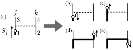
The whole update process of the world-line configuration consists of the diagonal update and the worm update Kawashima and Harada (2004). In the former, the diagonal bond operators in the Hamiltonian (10) are inserted into or removed from a world-line configuration according to the diagonal elements. In the latter, first a worm, i.e., a pair of the raising and lowering operators, is inserted at a randomly chosen space-time point, and either operator is chosen as the head. The order of the ladder operators is uniquely determined in the case with $S=1/2$ since the local degree of freedom is binary (up or down). The worm head then moves along the imaginary-time direction until it arrives at a bond operator. At the operator, the worm head is scattered and its moving direction and/or sitting site may be changed stochastically according to the matrix elements (14). In Fig. 2, an example of the worm-scattering process is illustrated. We choose transition probabilities so as to minimize the bounce probability (see Fig. 2), by breaking both the detailed balance of each worm-scattering process and even that of the whole Monte Carlo dynamics Suwa and Todo (2010). This scattering process is repeated until the worm head reaches back its own tail. Then the head and tail destroy each other. The worm is inserted at several times in each Monte Carlo step.

Fig 2: Example of the worm scattering process. The bold line denotes a string of $S^{z}=1/2$ states (or the path of the worm head), while the thin line does $S^{z}=-1/2$ states. The dotted line expresses a bond operator. When the worm head, $S_{j}^{-}$, (a) arrives at leg 1 of the bond operator, one of the following events will occur. The head (b) bounces back to the way which it comes from, (c) goes straight and gets out from leg 3, (d) jumps to leg 4, or (e) turns to leg 2. The transition probabilities in the scattering process are determined by the matrix elements (14). In the present model, event (e) never occurs due to the total $S^{z}$ conservation.

We will investigate the phase transition between the $xy$-plane ferromagnetic phase and the disordered phase. The order parameter is the transverse (off-diagonal) magnetization in $x$ or $y$ direction. Although it is non-trivial to measure off-diagonal correlation in a WLQMC simulation, one can efficiently calculate the structure factor

$$S_{0}=\frac{1}{L^{2}}\Big{\langle}\sum_{j,k}(S_{j}^{x}S_{k}^{x}+S_{j}^{y}S_{k}^{y})\Big{\rangle},$$ (15)

the transverse susceptibility

$$\chi=\frac{1}{L^{2}\beta}\Big{\langle}\sum_{j,k}\int_{0}^{\beta}\!\!{\mathrm{d}}\tau_{1}\int_{0}^{\beta}\!\!{\mathrm{d}}\tau_{2}\,S_{j}^{+}(\tau_{1})S_{k}^{-}(\tau_{2})\Big{\rangle},$$ (16)

and the Fourier component of the (spatial and temporal) correlation functions, exploiting the virtue of the worm-update process Prokof’ev et al. (1998). Here the symbols are defined as follows: $\langle O\rangle=\mathrm{Tr}[O\mathrm{e}^{-\beta H}]/Z$ and $O(\tau)=\mathrm{e}^{-\tau H}O\mathrm{e}^{\tau H}$. The correlation lengths in $x$, $y$, and $\tau$ directions are then calculated from the Fourier components by the second-moment method Cooper et al. (1982); Todo and Kato (2001). The detail of the measurement of these quantities is explained in Appendix B.

At the critical point, the structure factor and the susceptibility exhibit the following power-law behavior:

$$S_{0}(L)\propto L^{\theta},$$ (17)

and

$$\chi(L)\propto L^{\gamma/\nu},$$ (18)

respectively. Here we introduce $\theta\equiv 2-2{\beta}/\nu$, where $\beta$ is not the inverse temperature but the critical exponent of the order parameter. The exponent of the susceptibility is denoted by $\gamma$. Note that in Eqs. (8), (17), and (18), one can use the quantities evaluated at $g_{\mathrm{c}}(L)$, the solution of Eqs. (5) and (6) for each system size $L$, instead of the true critical point $g_{\mathrm{c}}$, as both give the same exponent.

IV Numerical results

IV.1 For $h^{\mathrm{u}}=0$

First we discuss the case without the uniform magnetic field. We performed WLQMC simulations for system sizes $L=8,\cdots,64$, and obtained the optimal inverse temperature $\beta(L)$ and staggered magnetic field $h^{\mathrm{s}}_{\mathrm{c}}(L)$ for each $L$ by solving Eqs. (5) and (6) using the stochastic approximation. The optimal inverse temperature $\beta(L)$ ensures that the system is virtually isotropic, and the optimal staggered magnetic field $h^{\mathrm{s}}_{\mathrm{c}}(L)$ gives an estimate of the critical point. The target relative correlation lengths, $R$ and $R_{\tau}$, were chosen as $R=R_{\tau}=0.5$, $R_{XY}$, or 0.7, where $R_{XY}=0.5925$ is the approximate value of $\lim_{L\rightarrow\infty}\xi(L)/L$ at the critical point of the three-dimensional classical $XY$ model Campostrini et al. (2001). Note that a particular choice of $R$ and $R_{\tau}$ does not introduce any bias to the final estimates; it affects only the speed of convergence to the thermodynamic limit as seen below.

Fig 3: (Color online) System-size dependence of the critical staggered field, $h^{\mathrm{s}}_{\mathrm{c}}(L)$, for $h^{\mathrm{u}}=0$. The extrapolated value is $h^{\mathrm{s}}_{\mathrm{c}}=0.99179(3)$, and the lines are the bootstrapped fitting curves (see the body).

Fig 4: (Color online) System-size dependence of the transverse susceptibility (16), the structure factor (15), and the inverse temperature at $h^{\mathrm{s}}_{\mathrm{c}}(L)$ for $h^{\mathrm{u}}=0$. The red squares, green circles, and blue triangles are the data plots for $R=0.5$, $R_{XY}$, and $0.7$, respectively.

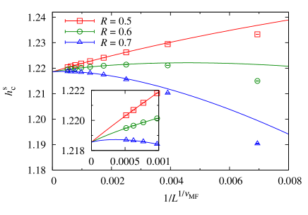
The critical strength of the staggered magnetic field, $h^{\mathrm{s}}_{\mathrm{c}}$, can be estimated based on the asymptotic form (7), i.e.,

$$h^{\mathrm{s}}_{\mathrm{c}}(L)=h^{\mathrm{s}}_{\mathrm{c}}+c(R)L^{-1/\nu},$$ (19)

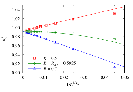
where $c(R)$ is a certain constant which depends only on $R$ ($=R_{\tau}$, here). The system-size dependence of $h^{\mathrm{s}}_{\mathrm{c}}(L)$ is shown in Fig. 3. We extrapolated the critical point from the finite-size data by using the ansatz Eq. (19) and assuming the same $h^{\mathrm{s}}_{\mathrm{c}}$ for three different values of $R$. Seven parameters, $h^{\mathrm{s}}_{\mathrm{c}}$ and ($c(R)$, $\nu(R)$) for each $R$, were determined by the least squares fitting. (Note that also $\nu(R)$ is a fitting parameter in our analysis.) In order to estimate the statistical error, we performed the following bootstrap procedure. From several hundreds Robbins-Monro runs, the physical quantities and the parameters [$\beta(L)$ and $h^{\mathrm{s}}_{\mathrm{c}}(L)$] were obtained with some statistical error bars. Then the data were resampled from the Gaussian distribution with the estimated mean and variance. The generated samples were fitted for large-enough system-size data that minimize $\chi^{2}/\mathrm{d.o.f}$, where the asymptotic form (19) would approximate the plots well (we used the data for $L\in[24,64]$ and obtained $\chi^{2}/\mathrm{d.o.f.}\approx 2.0$). This procedure was repeated 4000 times, which yielded as many fitted functions. By taking the average of the function values, we obtained a whole shape of $h^{\mathrm{s}}_{\mathrm{c}}(L)$ that should be asymptotically accurate, which is shown in Fig. 3 as the solid line for each $R$. Finally, the bootstrap estimation gave the critical point $h^{\mathrm{s}}_{\mathrm{c}}=0.99179(3)$ for $h^{\mathrm{u}}=0$, where the number in the parenthesis denotes the standard error of the estimation in the last digit(s). It is consistent with the previous report, $h^{\mathrm{s}}_{\mathrm{c}}=0.9919(4)$ Priyadarshee et al. (2006), but more precise by an order of magnitude.

It should be noted that in Fig. 3 the fastest convergence is achieved by the choice of $R=R_{XY}$, i.e., the leading correction seems $o(1/L^{1/\nu_{XY}})$ at $R=R_{XY}$. Meanwhile, the leading correction is likely in the order of $1/L^{1/\nu_{XY}}$ at $R=0.5$ and $0.7$, where $\nu_{XY}=0.67155$ Campostrini et al. (2001) is the critical exponent of the correlation length for the 3D-$XY$ universality class. These findings indicate that this phase transition belongs to the 3D-$XY$ universality class.

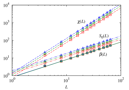
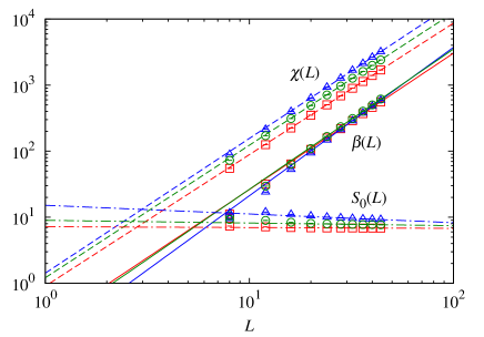
In Fig. 4, we present the system-size dependence of the inverse temperature, the static structure factor, and the transverse susceptibility. Assuming the asymptotic forms [Eqs. (8), (17), and (18)], we conclude $z=0.992(6)$, $\gamma/\nu=1.967(6)$, and $\theta=0.968(5)$. These results are fully consistent with the scenario of the 3D-$XY$ universality class, $\gamma/\nu=1.9620(4)$ and $\theta=0.9620(4)$ Campostrini et al. (2001), with $z=1$. The final estimates for $z$, $\theta$, and $\gamma/\nu$, which were evaluated from the asymptotic behavior of the different quantities, indeed satisfy the scaling relation

$$\gamma/\nu=\theta+z$$ (20)

within the error bar.

Fig 5: (Color online) System-size dependence of the critical staggered field $h^{\mathrm{s}}_{\mathrm{c}}(L)$ for $h^{\mathrm{u}}=0.5$. The extrapolated value is $h^{\mathrm{s}}_{\mathrm{c}}=1.21855(2)$. The lines were obtained by the same bootstrap approach with $h^{\mathrm{u}}=0$ (see the body). The inset shows the detail of the extrapolation for larger $L$.

Fig 6: (Color online) System-size dependence of the transverse susceptibility (16), the structure factor (15), and the inverse temperature at $h^{\mathrm{s}}_{\mathrm{c}}(L)$ for $h^{\mathrm{u}}=0.5$. The red squares, green circles, and blue triangles are the data plots for $R=0.5$, $0.6$, and $0.7$, respectively.

Fig 7: (Color online) Finite-size corrections of the critical exponents: (a) the dynamical exponent, $z$, (b) the exponent of the susceptibility, $\gamma/\nu$, and (c) that of the structure factor, $\theta$. Each data point represents the exponent obtained by the fit for each triad (see the body).

IV.2 For $h^{\mathrm{u}}=0.5$

Next, we discuss the critical point and the critical exponents for the case with finite uniform magnetic field $h^{\mathrm{u}}=0.5$. In this case we used $R=0.5$, $0.6$, and $0.7$ for $L=8,12,16,20,24,28,32,36,40,44$. Following the same procedure with the case for $h^{\mathrm{u}}=0$, we obtained $h^{\mathrm{s}}_{\mathrm{c}}=1.21855(2)$, the quantum critical point. In the fitting procedure, the data with $L\in[24,44]$ were used ($\chi^{2}/\mathrm{d.o.f.}\approx 0.8$).

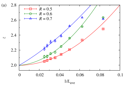
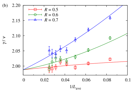
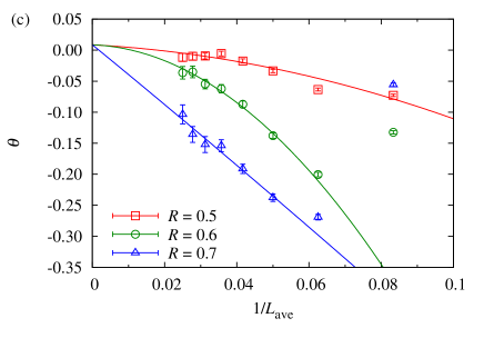
The system-size dependence of the physical quantities is shown in Fig. 6. In comparison to the case with $h^{\mathrm{u}}=0$ shown in Fig. 4, larger corrections to scaling are seen, especially for $\beta(L)$. To cope with the strong finite-size corrections, we took the following procedure: Assume we have data points at system sizes $L=L_{1}$, $L_{2}$, $\cdots$, $L_{n}$, where $L_{1}<L_{2}<\cdots<L_{n}$. First, we construct triads consisting of the data with three consecutive system sizes as $(L_{1},L_{2},L_{3})$, $(L_{2},L_{3},L_{4})$, $\cdots$, and $(L_{n-2},L_{n-1},L_{n})$, defining $L_{\mathrm{ave}}$ as the average system size of each triad. Next, we fit each triad with a simple power function, i.e., $y(L)=a(L_{\mathrm{ave}})\times L^{b(L_{\mathrm{ave}})}$ with $a(L_{\mathrm{ave}})$ and $b(L_{\mathrm{ave}})$ the fitting parameters depending on $L_{\mathrm{ave}}$. The error of $b(L_{\mathrm{ave}})$ is estimated by the bootstrap method as explained above. Then, we fit $b(L_{\mathrm{ave}})$ with a quadratic function of $1/L_{\mathrm{ave}}$, and extrapolate the critical exponent in the thermodynamic limit. In our fitting procedure of the exponent, we assume that the fitting function should be monotonic.

The extrapolation results are shown in Fig. 7. For the dynamical exponent, we estimated $z=2.00(2)$; the effective dimension of the imaginary-time axis changes from one to two by the introduction of uniform magnetic field $h^{\mathrm{u}}$. As for the other critical exponents, $\gamma/\nu=1.99(1)$ and $\theta=0.01(1)$ were obtained. These values coincide with the mean-field exponents, i.e., $\gamma/\nu=2$ and $\theta=0$. This is consistent with the result for the dynamical exponent, $z=2$, by which the effective dimension of the critical theory becomes four, the upper critical dimension. Thus we have demonstrated that our finite-size scaling method enables us to extract the dynamical exponent successfully without any prior knowledge of the value of $z$. The universality of the quantum phase transition without particle-hole symmetry belongs to the mean-field universality class. This is consistent with the discussion on the Bose-Hubbard model in Ref. 7.

V Summary and discussions

In the present paper, we have presented the unified finite-size scaling method that works well regardless of the value of the dynamical exponent. During the WLQMC simulation, the system size in the imaginary-time direction in the path-integral representation is adjusted automatically so as to satisfy the conditions, $\xi/L=R$ and $\xi_{\tau}/\beta=R_{\tau}$, based on the Robbins-Monro stochastic approximation. This auto-tuning procedure guarantees that the coupling constant converges to the critical point and the inverse temperature is proportional to $L^{z}$ for large enough $L$.

We then applied the method to the two-dimensional $S=1/2$ quantum $XY$ model in uniform and staggered magnetic fields. The correlation lengths were measured by the worm algorithm based on the continuous imaginary-time representation. In the absence of the uniform magnetic field, $h^{\mathrm{u}}=0$, our numerical results are consistent with the 3D-$XY$ universality class. This system can be mapped into the half-filled hard-core boson system. The Lorentz invariance, $z=1$, reflects the particle-hole symmetry at half-filling. In the case with $h^{\mathrm{u}}=0.5$, we have concluded that the dynamical exponent changes to two and the other exponents take the mean-field values. This result of the mean-field universality is consistently explained by the conclusion that the dimension of the effective field theory is four; $d+z=4$, the upper critical dimension. Our conclusion $z=2$ agrees on the discussion in Ref. 7, in which the authors claimed that the fourth-order term in the effective action becomes irrelevant.

The method proposed in the present paper is applicable also to models with randomness. For example, the method will be effective for systems whose dynamical exponent depends on the parameters, such as the random Ising model in random transverse field Pich et al. (1998); Rieger and Kawashima (1999), where the dynamical exponent may take an irrational value or even becomes infinite Fisher (1995). It is thus extremely difficult to analyze the properties of quantum criticality by the conventional strategies. By using our method, one does not need any assumption about the dynamical exponent, which should be quite effective for the systematic investigation of the randomness-driven quantum critical point causing extreme space-time anisotropy.

Appendix A Convergence by the Robbins-Monro algorithm

Fig 8: (Color online) Convergence of the (a) bias and (b) variance for solving $f(\beta)=\exp(\beta)-1=0$ with the initial condition $\beta^{(1)}=\beta_{\mathrm{init}}=1$. At the $n$-th RMS, a value (corresponding to the relative correlation length in the quantum-phase-transition analyses) is generated from the normal distribution, $\mathcal{N}(f(\beta^{(n)}),0.1)$. Note that $a=1$ in this case. The results for $p=0.1$, $0.3$, $0.5$, $1.0$, $2.0$, and $5.0$ are shown (calculated from $10^{8}$ Robbins-Monro processes). As shown in the text, the variance is minimized by the choice of $p=1/a=1$ at large enough RMSs, while the bias convergence is accelerated monotonically with respect to $p$.

In this appendix, the time evolution of the probability distribution function driven by the Robbins-Monro iteration [Eq. (9)] is discussed. Let us consider the situation in which the physical quantity $A(\beta)$ is obtained by Monte Carlo simulation and the distribution function of $A(\beta)$ is given by a Gaussian (normal) distribution written as

$$P(A) =\mathcal{N}(f(\beta),\sigma^{2})$$

$$=\frac{1}{\sqrt{2\pi\sigma^{2}}}\exp\left[-\frac{(A-f(\beta))^{2}}{2\sigma^{2}}\right].$$ (21)

Also, we assume that $f(\beta)$ can be expanded as

$$f(\beta)\approx a(\beta-\beta_{\mathrm{c}}),$$ (22)

near $\beta_{\mathrm{c}}$, the zero of $f(\beta)$. Then, the asymptotic recursion relation between the distribution functions of $\beta^{(n)}$ and $\beta^{(n+1)}$ is written as

$$P_{n+1}(\beta^{(n+1)})\propto\int{\mathrm{d}}\beta^{(n)}P_{n}(\beta^{(n)})$$

$$\times\exp\left\{-\frac{1}{2\sigma^{2}}\left[\frac{n}{p}(\beta^{(n)}-\beta^{(n+1)})-a(\beta^{(n)}-\beta_{\mathrm{c}})\right]^{2}\right\}.$$ (23)

In our procedure, we start from an initial condition $P_{1}(\beta^{(1)})=\delta(\beta^{(1)}-\beta_{\mathrm{init}})$. Here we assume that the distribution function of $P_{n}(\beta^{(n)})$ will be approximated by a Gaussian for large enough $n$. Then the recursion relations for the mean, $\mu_{n}$, and the variance, $\sigma_{n}^{2}$, of $P_{n}(\beta^{(n)})$ are obtained as

$$\mu_{n+1}=\left(1-\frac{ap}{n}\right)\mu_{n}+\frac{ap}{n}\beta_{\mathrm{c}}$$ (24)

$$\sigma_{n+1}^{2}=\sigma^{2}\left(\frac{p}{n}\right)^{2}+\sigma_{n}^{2}\left(1-\frac{ap}{n}\right)^{2},$$ (25)

respectively. Eq. (24) can be rewritten as

$$\mu_{n+1}-\beta_{\mathrm{c}}=\left(1-\frac{ap}{n}\right)\left(\mu_{n}-\beta_{\mathrm{c}}\right).$$ (26)

The absolute value of $(1-ap/n)$ in Eq. (26) is less than 1 for sufficiently large $n$. Then $\mu_{n}\rightarrow\beta_{\mathrm{c}}$ for $n\to\infty$. Similarly, it can be proved that $\sigma_{n}^{2}\to 0$ for $n\to\infty$.

Next, let us assume the leading term of $\sigma_{n}^{2}$ as ${s^{2}}/{n^{\alpha_{s}}}$, where $\alpha_{s}$ is an unknown constant and $s^{2}$ is the asymptotic variance of $\sigma_{n}^{2}$. From the approximation $(n+1)^{-\alpha_{s}}\approx n^{-\alpha_{s}}(1-\alpha_{s}/n)$ for $n\gg 1$, the lowest-order terms in Eq. (25) are evaluated as

$$-\frac{s^{2}\alpha_{s}}{n^{\alpha_{s}+1}}\approx\frac{\sigma^{2}p^{2}}{n^{2}}-\frac{2s^{2}ap}{n^{\alpha_{s}+1}}.$$ (27)

When $\alpha_{s}<1$, $1/n^{\alpha_{s}+1}$ dominates over $1/n^{2}$. Then $\alpha_{s}=2ap$ and

$$\sigma_{n}^{2}\sim\frac{1}{n^{2ap}}\qquad\text{for $ap<\frac{1}{2}$.}$$ (28)

When $\alpha_{s}=1$, on the other hand,

$$\sigma_{n}^{2}\approx\frac{s^{2}}{n}=\frac{1}{n}\frac{\sigma^{2}p^{2}}{2ap-1}\qquad\text{for $ap>\frac{1}{2}$.}$$ (29)

There is no solution under the assumption as for the case where $ap=1/2$, but it is expected that only some correction from $\sigma_{n}^{2}\sim 1/n$ will appear.

Similar discussion holds for the mean of distribution, $\mu_{n}$. Assuming $\mu_{n}-\beta_{\mathrm{c}}=k/n^{\alpha_{m}}$, with some constants $k$ and $\alpha_{m}$, we obtain

$$\beta_{\mathrm{c}}+\frac{k}{n^{\alpha_{m}}}\left(1-\frac{\alpha_{m}}{n}\right)=\left(1-\frac{ap}{n}\right)\left(\beta_{\mathrm{c}}+\frac{k}{n^{\alpha_{m}}}\right)+\frac{ap}{n}\beta_{\mathrm{c}}$$ (30)

from Eq. (24). This results in $\alpha_{m}=ap$, and thus we have

$$\mu_{n}-\beta_{\mathrm{c}}\sim\frac{1}{n^{ap}}\qquad\text{for $ap>0$.}$$ (31)

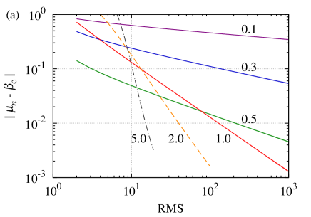
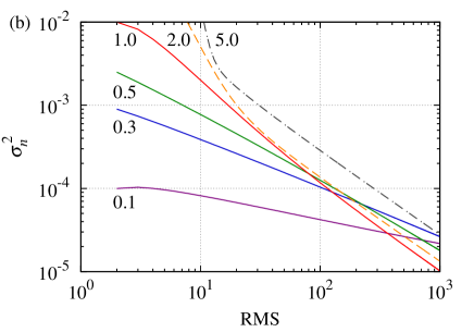
According to the asymptotic forms (28), (29), and (31), let us discuss the dependence of the final error on the number of Monte Carlo steps. It is obvious from Eqs. (28) and (29) that it is better to set the gain $|p|$ large enough so that $ap>1/2$ is satisfied. Otherwise the convergence of the variance becomes slower. We will call one iteration of the Robbins-Monro feedback process [Eq. (9)] a Robbins-Monro step (RMS), and suppose that a whole calculation consists of $N_{\mathrm{R}}$ RMSs and each RMS has $N_{\mathrm{M}}$ Monte Carlo updates. The total computational cost is proportional to $N_{\mathrm{tot}}\equiv N_{\mathrm{R}}\times N_{\mathrm{M}}$. From Eq. (29), the variance of the estimate after $N_{\mathrm{R}}$ RMSs is given by $\sigma_{N_{\mathrm{R}}}\approx s^{2}/N_{\mathrm{R}}\sim\sigma^{2}/N_{\mathrm{R}}$ for $ap>1/2$. Using $\sigma^{2}\approx s^{2}_{\mathrm{MC}}/N_{\mathrm{M}}$, where $s^{2}_{\mathrm{MC}}$ is the asymptotic variance of the Monte Carlo estimation, we obtain

$$\sigma_{N_{\mathrm{R}}}\sim\frac{s^{2}_{\mathrm{MC}}}{N_{\mathrm{tot}}}.$$ (32)

This means that the asymptotic variance depends only on the total number of Monte Carlo updates $N_{\mathrm{tot}}$.

Next, let us discuss the optimal choice of the gain $p$. For $ap>1/2$, the convergence of $\mu_{n}$ is faster than that of $\sigma_{n}$. Thus, we should minimize $\sigma_{n}$ in Eq. (29); then we derive

$$p=\frac{1}{a}.$$ (33)

Fig. 8 shows the $p$ dependence of $\mu_{n}$ and $\sigma_{n}^{2}$ calculated from an exemplary case:

$$f(\beta)=\exp(\beta)-1,$$ (34)

where $\beta_{\mathrm{c}}=0$ and $a=1$. While the convergence of the mean becomes faster monotonically as $p$ increases, the variance takes a minimum value at $p=1/a=1$ and increases again for larger $p$. In the simulation presented in the main text, we performed short preparatory calculations for small systems in order to roughly estimate $a\approx a^{*}$, and set $p=1/a^{*}$ for succeeding long runs. We performed several hundreds of Robbins-Monro iterations, each of which has $N_{\mathrm{M}}=500$ worm updates.

Appendix B Measurement of off-diagonal correlation in the worm algorithm

We explain the way to measure off-diagonal correlation in the worm algorithm. Let us begin with measuring the static structure factor defined in Eq. (15). This quantity is easily rewritten by the spin raising and lowering operators. We then need to evaluate the thermal average,

$$\Big{\langle}\sum_{j,k}S_{j}^{+}S_{k}^{-}\Big{\rangle}=\frac{\mathrm{Tr}\Big{[}\sum_{j,k}S_{j}^{+}S_{k}^{-}\mathrm{e}^{-\beta\mathcal{H}}\Big{]}}{\mathrm{Tr}\,\mathrm{e}^{-\beta\mathcal{H}}}.$$ (35)

The numerator and denominator in Eq. (35) correspond to the partition function of extended world-line configurations with a worm and those of the original world-line configurations, respectively. In other words, Eq. (35) can be read as the frequency of events that the worm head visits the same imaginary time with the tail. We thus can measure the static structure factor by simply counting the frequency of extended configurations that contribute to the numerator in Eq .(35) during each worm update.

We have also evaluated the dynamic structure factor at imaginary frequency $i\omega$. It is given by the canonical correlation function as

$$C(\vec{q},i\omega) =\frac{1}{L^{2}\beta}\Big{\langle}\sum_{j,k}\int_{0}^{\beta}\!\!\mathrm{d}\tau_{1}\int_{0}^{\beta}\!\!\mathrm{d}\tau_{2}\,S_{j}^{+}(\tau_{1})S_{k}^{-}(\tau_{2})$$

$$\times\exp\left\{-i\left[\omega(\tau_{2}-\tau_{1})+\vec{q}\cdot(\vec{r}_{k}-\vec{r}_{j})\right]\right\}\Big{\rangle},$$ (36)

where $i\omega=2\pi i/\beta$ is the lowest Matsubara frequency in our simulation. The spatial phase factor $\mathrm{e}^{-i\vec{q}\cdot(\vec{r}_{k}-\vec{r}_{j})}$ can be calculated and stored in advance. Then, when the head moves in the worm-update process, the imaginary-time integral is evaluated. In simulations, every time the head reaches a bond operator, a part of the imaginary-time integral is performed. Since the $\tau$-dependent part of the integrand is simply given by $\mathrm{e}^{i\omega\tau}$, we can evaluate the part of the integral exactly at each head move. The spatial phase factor is multiplied (if necessary). The matrix elements of the head and tail also need to be considered (they are simply one in the case with $S=1/2$). The contribution to the integral at each head move is summed up until the head returns back to its tail. The average value of the summed integral for each worm insertion will provide the target quantity (36).

The transverse susceptibility (16) is expressed as $\chi=C(\vec{0},0)$. The correlation length can be estimated by the second-moment method Cooper et al. (1982); Todo and Kato (2001); the correlation length in the $x$ direction, $\xi_{x}$, is expressed as

$$\xi_{x}=\frac{1}{|\delta\vec{q}_{x}|}\sqrt{\frac{C(\vec{q}_{0},0)}{C(\vec{q}_{0}+\delta\vec{q}_{x},0)}-1},$$ (37)

where $\delta\vec{q}_{x}=(2\pi/L,0)$ and $\vec{q}_{0}=(0,0)$. Similarly, the correlation length in the imaginary-time direction, $\xi_{\tau}$, as

$$\xi_{\tau}=\frac{1}{\omega}\sqrt{\frac{C(\vec{q}_{0},0)}{C(\vec{q}_{0},i\omega)}-1}.$$ (38)

References

- Sachdev (1999) S. Sachdev, Quantum Phase Transition (Cambridge University Press, Cambridge, 1999).
- Avella and Mancini (2013) A. Avella and F. Mancini, eds., Strongly Correlated Systems: Numerical Methods (Springer-Verlag, Berlin, 2013).
- Suzuki (1976) M. Suzuki, Prog. Theor. Phys. 56, 1454 (1976).
- Vojta (2003) M. Vojta, Rep. Prog. Phys. 66, 2069 (2003).
- Suzuki (1994) M. Suzuki, ed., Quantum Monte Carlo Methods in Condensed Matter Physics (World Scientific, Singapore, 1994).
- Landau and Binder (2005) D. P. Landau and K. Binder, A Guide to Monte Carlo Simulations in Statistical Physics, 2nd ed. (Cambridge University Press, Cambridge, 2005).
- Fisher et al. (1989) M. P. A. Fisher, P. B. Weichman, G. Grinstein, and D. S. Fisher, Phys. Rev. B 40, 546 (1989).
- Singh and Rokhsar (1992) K. G. Singh and D. S. Rokhsar, Phys. Rev. B 46, 3002 (1992).
- Herbut (1997) I. F. Herbut, Phys. Rev. Lett. 79, 3502 (1997).
- Weichman and Mukhopadhyay (2007) P. B. Weichman and R. Mukhopadhyay, Phys. Rev. Lett. 98, 245701 (2007).
- Sørensen et al. (1992) E. S. Sørensen, M. Wallin, S. M. Girvin, and A. P. Young, Phys. Rev. Lett. 69, 828 (1992).
- Zhang et al. (1995) S. Zhang, N. Kawashima, J. Carlson, and J. E. Gubernatis, Phys. Rev. Lett. 74, 1500 (1995).
- Prokof’ev and Svistunov (2004) N. Prokof’ev and B. Svistunov, Phys. Rev. Lett. 92, 015703 (2004).
- Priyadarshee et al. (2006) A. Priyadarshee, S. Chandrasekharan, J.-W. Lee, and H. U. Baranger, Phys. Rev. Lett. 97, 115703 (2006).
- Meier and Wallin (2012) H. Meier and M. Wallin, Phys. Rev. Lett. 108, 055701 (2012).
- Álvarez Zúñiga et al. (2015) J. P. Álvarez Zúñiga, D. J. Luitz, G. Lemarié, and N. Laflorencie, Phys. Rev. Lett. 114, 155301 (2015).
- Hüvonen et al. (2012) D. Hüvonen, S. Zhao, M. Månsson, T. Yankova, E. Ressouche, C. Niedermayer, M. Laver, S. N. Gvasaliya, and A. Zheludev, Phys. Rev. B 85, 100410(R) (2012).
- Yu et al. (2012) R. Yu, C. F. Miclea, F. Weickert, R. Movshovich, A. Paduan-Filho, V. S. Zapf, and T. Roscilde, Phys. Rev. B 86, 134421 (2012).
- Rieger and Young (1994) H. Rieger and A. P. Young, Phys. Rev. Lett. 72, 4141 (1994).
- Pich et al. (1998) C. Pich, A. P. Young, H. Rieger, and N. Kawashima, Phys. Rev. Lett. 81, 5916 (1998).
- Pollet (2013) L. Pollet, Comptes Rendus Physique 14, 712 (2013).
- Jiang (2011) F.-J. Jiang, Phys. Rev. B 83, 024419 (2011).
- Jiang (2012) F.-J. Jiang, Phys. Rev. B 85, 014414 (2012).
- Machta et al. (1995) J. Machta, Y. S. Choi, A. Lucke, T. Schweizer, and L. V. Chayes, Phys. Rev. Lett. 75, 2792 (1995).
- Tomita and Okabe (2001) Y. Tomita and Y. Okabe, Phys. Rev. Lett. 86, 572 (2001).
- Wang and Landau (2001) F. Wang and D. P. Landau, Phys. Rev. Lett. 86, 2050 (2001).
- Yasuda and Todo (2013) S. Yasuda and S. Todo, Phys. Rev. E 88, 061301(R) (2013).
- Wenzel and Janke (2009) S. Wenzel and W. Janke, Phys. Rev. B 79, 014410 (2009).
- Wenzel et al. (2008) S. Wenzel, L. Bogacz, and W. Janke, Phys. Rev. Lett. 101, 127202 (2008).
- Robbins and Monro (1951) H. Robbins and S. Monro, Ann. Math. Stat. 22, 400 (1951).
- Bishop (2006) C. M. Bishop, Pattern Recognition and Machine Learning (Springer, New York, 2006).
- Albert and Gardner (1970) A. E. Albert and L. A. Gardner, Stochastic Approximation and Nonlinear Regression (MIT Press, Cambridge, 1970).
- Lieb et al. (1961) E. Lieb, T. Schultz, and D. Mattis, Annals of Physics 16, 407 (1961).
- Hen et al. (2010) I. Hen, M. Iskin, and M. Rigol, Phys. Rev. B 81, 064503 (2010).
- Hen and Rigol (2009) I. Hen and M. Rigol, Phys. Rev. B 80, 134508 (2009).
- Prokof’ev et al. (1998) N. V. Prokof’ev, B. V. Svistunov, and I. S. Tupitsyn, Sov. Phys. JETP 87, 310 (1998).
- Syljuasen and Sandvik (2002) O. F. Syljuasen and A. W. Sandvik, Phys. Rev. E 66, 046701 (2002).
- Kawashima and Harada (2004) N. Kawashima and K. Harada, J. Phys. Soc. Jpn. 73, 1379 (2004).
- Suwa and Todo (2010) H. Suwa and S. Todo, Phys. Rev. Lett. 105, 120603 (2010).
- Cooper et al. (1982) F. Cooper, B. Freedman, and D. Preston, Nucl. Phys. B 210[FS6], 210 (1982).
- Todo and Kato (2001) S. Todo and K. Kato, Phys. Rev. Lett. 87, 047203 (2001).
- Campostrini et al. (2001) M. Campostrini, M. Hasenbusch, A. Pelissetto, P. Rossi, and E. Vicari, Phys. Rev. B 63, 214503 (2001).
- Rieger and Kawashima (1999) H. Rieger and N. Kawashima, Eur. Phys. J. B 9, 233 (1999).
- Fisher (1995) D. S. Fisher, Phys. Rev. B 51, 6411 (1995).
- (45) “http://github.com/wistaria/worms,” .
- Bauer and et al. (2011) B. Bauer and et al., J. Stat Mech. , P05001 (2011).
- (47) “http://alps.comp-phys.org/,” .
- (48) “http://github.com/cmsi/bcl,” .